Stable and metastable phases for the Curie-Weiss-Potts model in vector-valued fields via singularity theory

Abstract

We study the metastable minima of the Curie-Weiss Potts model with three states, as a function of the inverse temperature, and for arbitrary vector-valued external fields. Extending the classic work of [7] and [28] we use singularity theory to provide the global structure of metastable (or local) minima. In particular, we show that the free energy has up to four local minimizers (some of which may at the same time be global) and describe the bifurcation geometry of their transitions under variation of the parameters.

Keywords:

Potts model, metastable minima, singularity theory, singularity set, bifurcation set, butterfly, elliptic umbilic

1 Introduction

1.1 Research context

The Potts model [29], and in particular its Curie-Weiss version, is next to the Curie-Weiss Ising model, one of the most studied models in statistical mechanics. While basic aspects of Curie-Weiss models can be discovered by ad-hoc computations, they provide ongoing challenges for refined problems involving dynamics, metastability, complex parameters, fine asymptotics [[, see for example]]Cerf_2016, fernandez12, chatterjee11, gheissari18, shamis17, Eichelsbacher_2015, landim16_metas_non_rever_mean_field. In particular, motivated by metastability one aims at a full understanding of the free energy landscape [25, 2]. The phase-diagram for the stable states of the Curie-Weiss Potts model, that is the behaviour of global minimizers, is known and described by the Ellis-Wang theorem [7] in zero external field. [28] provides some results in non-zero external field relating to global minimizers.

For the metastable states, that is, the local minima and their transitions a complete exposition of the global analysis in the whole parameter space, revealing the full structure of their transitions is lacking in the literature. See [12, 13, 14] for a partial analysis based on polynomial equivalence given for some regions in parameter space.

One is not just interested in the static behaviour of the model, but also in the behaviour under stochastic dynamics, in and out of equilibrium, where we see next to metastability also the phenomenon of dynamical Gibbs – non-Gibbs transitions [[, see]]van_Enter_2010_Kuelske_Opoku_Ruszel, Kissel_2020, EnFeHoRe, van_Enter_Ermolaev_Iacobelli_Kuelske_2012, Jahnel_2017. Employing the probabilistic notion of sequential Gibbs property, such dynamical Gibbs – non-Gibbs transitions have been shown to occur and analyzed for a number of exchangeable models in [21, 18, 20]. A way to understand these transitions for independent dynamics is to examine the structure of stationary points of a conditional rate function which generalizes the equilibrium rate function but contains more information. This conditional rate function depends on all model parameters of the static model, but has an additional time-parameter, and a measure-valued parameter with the meaning of an empirical distribution. We are planning to investigate the time-evolved Curie-Weiss Potts model in the spirit of [21, 11, 16]. For this the analysis of the static problem for general parameter values (which means for general vector-valued fields) is a necessary first step.

As a guiding principle for such analysis, singularity theory is very useful to understand the organization of stationary points for varying parameters. It allows to understand and discover the types of local bifurcations which are present in the applied problem as (by Thom’s theorem) they must be related via local diffeomorphisms to (partial) unfoldings of elementary singularities (so-called catastrophes). These catastrophes form prototypical types which in themselves can be most easily understood in polynomial models. Clear expositions describing their geometries are found in textbooks [26, 1, 24]. The simplest example is the rate function of the Curie-Weiss Ising model. It is even globally (for all values of inverse temperature and magnetic field, and all magnetizations) identical to one cusp singularity. As we will see, for the Potts model in a general field various triple points (where three local minima have merged) occur, and singularity theory becomes very useful if we want to understand the global picture of all the transitions the metastable minima undergo for general values of inverse temperature and fields which allow to lift all degeneracies.

The paper is organized as follows. As our main result we describe the geometry of the bifurcation set in the parameter space of inverse temperature and vector-valued fields (see Section 2). This decomposition of parameter space given by the bifurcation set provides a phase diagram describing also the metastable minima. We will show how some of the so-called elementary singularities (threefold symmetric butterflies and an elliptic umbilic surrounded by three folds) and their partial unfoldings beautifully interact and are glued together. We also describe the accompanying geometry of the free energy landscape for each connected component of the complement of the bifurcation set. Finally we complement the study with the description of the coexistence sets of lowest minima (Maxwell-sets) at which two, three, or four minima coexist (see Section 3).

1.2 Model

We consider the mean-field Potts model with three states and are interested in both the stable and metastable phases. Note that we sometimes use the term local minima to include both the global and local minima depending on the context. The space of configurations in finite-volume $n\geq 2$ is defined as $\Omega_{n}=\{1,2,3\}^{n}$. We define

$$\Delta^{2}=\{\nu\in\mathbb{R}^{3}\>|\>\nu_{i}\geq 0,\sum_{i=1}^{3}\nu_{i}=1\}$$ (1)

and often refer to it as the unit simplex. The Hamiltonian of this model is given by

$$H_{n}(\sigma)=-\frac{1}{2n}\sum_{i,j=1}^{n}\delta_{\sigma_{i},\sigma_{j}}$$ (2)

where $\sigma$ lies in $\Omega_{n}$. The vector-valued fields are equivalently described by the a-priori measure $\alpha$ in the unit simplex $\Delta^{2}$. The finite-volume Gibbs distributions are therefore given by

$$\mu_{n,\beta,\alpha}(\sigma)=\frac{1}{Z_{n}(\beta,\alpha)}e^{-\beta H_{n}(\sigma)}\prod_{i=1}^{n}\alpha(\sigma_{i})$$ (3)

where the partition function is defined as

$$Z_{n}(\beta,\alpha)=\sum_{\sigma\in\Omega_{n}}e^{-\beta H_{n}(\sigma)}\prod_{i=1}^{n}\alpha(\sigma_{i}).$$ (4)

So the associated free energy in terms of the empirical spin distribution $\nu$ is given by

$$f_{\beta,\alpha}(\nu)=-\frac{1}{2}\beta\langle\nu,\nu\rangle+\sum_{i=1}^{3}\nu_{i}\log\frac{\nu_{i}}{\alpha_{i}}.$$ (5)

This is a real-valued function on the unit simplex $\Delta^{2}$ with two parameters: the inverse temperature $\beta$ and the external fields modeled by the a-priori measure $\alpha$. Thus, the parameter space is the product $(0,\infty)\times\Delta^{2}$. By a phase (stable or metastable) we mean a (global or local) minimizer of the free energy $f_{\beta,\alpha}$.

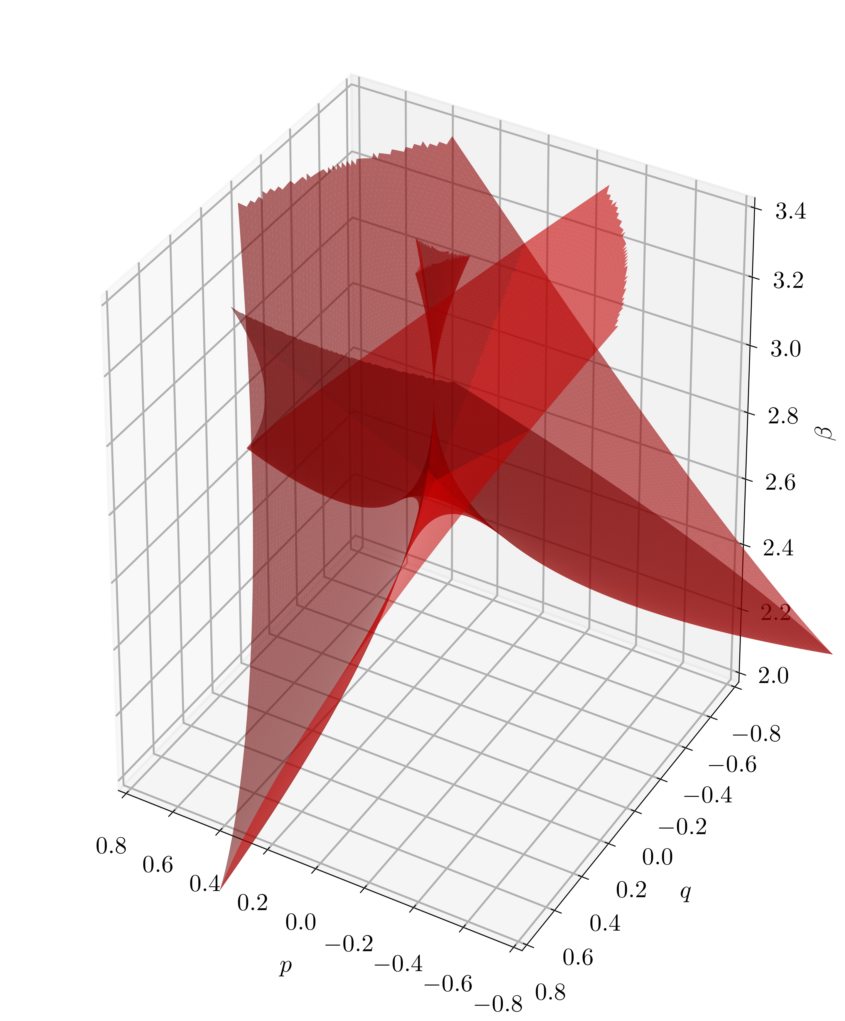
Figure 1: This plot shows the bifurcation set which is the basis for the metastable phase diagram. The surface shows pinches and self-intersections. Inside of the connected components of the complement the structure of metastable phases does not change. The unit simplex of a-priori measures $\alpha$ is embedded in the horizontal plane using the $(p,q)$-coordinates defined in (46).

2 The metastable phase diagram

In contrast to the usual question of phase-coexistence which is answered by the stable phase diagram (see Section 3), the metastable phase diagram contains information about the metastable phases of the system but not of their relative depth. Mathematically speaking, the metastable phase diagram is a partition of the parameter space whose cells contain parameter values $(\beta,\alpha)$ such that $f_{\beta,\alpha}$ has the same number of local minima. Using singularity theory we find that the metastable phase diagram is given by the connected complements of the surface shown in Figure 1. The structure of this union is particularly interesting because it shows features of two well-known catastrophes [26]: the butterfly catastrophe and the elliptic umbilic. The elliptic umbilic permits the change from minimum to maximum at the centre and is inherently associated to the Potts model because of its symmetry. The appearance of the butterfly is connected to triple points of Ising-like subsystems of the three-state Potts model. If we disfavor one of the three states, the remaining two act similarly to an Ising model in a random field. There is an interesting global interdependence of these two different catastrophes. We summarize the geometry of the extended phase diagram in the following theorem.

Theorem 1.

For each positive $\beta$ define the so-called catastrophe map $\chi_{\beta}$ from $\Delta^{2}$ to $\Delta^{2}$ which associates to each empirical spin distribution a $\beta$-dependent a-priori measure $\alpha$ modelling the external fields:

$$\chi_{\beta}(\nu)=\left(\frac{\nu_{i}e^{-\beta\nu_{i}}}{\sum_{k=1}^{3}\nu_{k}e^{-\beta\nu_{k}}}\right)_{i=1}^{3}$$ (6)

Define also curves $\gamma_{\beta}$ via

$$\gamma_{\beta}(x)=\frac{1}{2}\left(1-x-\sqrt{(1-x)^{2}-\frac{4(1-2\beta x(1-x))}{\beta(2-3\beta x)}}\right)$$ (7)

for $x\in D_{\beta}$ where the domain $D_{\beta}$ is a union of intervals given by

$$D_{\beta}=\begin{cases}\left(0,1-\frac{2}{\beta}\right]\cup\left(\frac{1}{2}-\frac{1}{2}\sqrt{1-\frac{2}{\beta}},\frac{1}{2}+\frac{1}{2}\sqrt{1-\frac{2}{\beta}}\right)&\text{if }2<\beta\leq\frac{8}{3},\\[9.0pt] \left(0,\frac{1}{2}-\frac{1}{2}\sqrt{1-\frac{2}{\beta}}\right)\cup\left(1-\frac{2}{\beta},\frac{1}{2}-\frac{1}{2}\sqrt{1-\frac{8}{3\beta}}\right)\\ \cup\left(\frac{1}{2}+\frac{1}{2}\sqrt{1-\frac{8}{3\beta}},\frac{1}{2}+\frac{1}{2}\sqrt{1-\frac{2}{\beta}}\right)&\text{if }\frac{8}{3}\leq\beta<3,\\[9.0pt] \left(0,\frac{1}{2}-\frac{1}{2}\sqrt{1-\frac{2}{\beta}}\right)\cup\left(\frac{1}{2}-\frac{1}{2}\sqrt{1-\frac{8}{3\beta}},1-\frac{2}{\beta},\right)\\ \cup\left(\frac{1}{2}+\frac{1}{2}\sqrt{1-\frac{8}{3\beta}},\frac{1}{2}+\frac{1}{2}\sqrt{1-\frac{2}{\beta}}\right)&\text{if }3\leq\beta.\end{cases}$$ (8)

Then consider the curve $\Gamma_{\beta}$ in $\Delta^{2}$ given by $\Gamma_{\beta}(x)=\chi_{\beta}(x,\gamma_{\beta}(x),1-x-\gamma_{\beta}(x))$ with $x\in D_{\beta}$. By $S_{3}\Gamma_{\beta}(D_{\beta})$ we denote the orbit of the curve $\Gamma_{\beta}$ under the action of the permutation group $S_{3}$ acting on $\Delta^{2}$.

1. The constant-temperature slices of the bifurcation set from Figure 1 are given by $S_{3}\Gamma_{\beta}(D_{\beta})$.

2. Table 1 shows an overview of the number of connected components of $S_{3}\Gamma_{\beta}(D_{\beta})$ together with the possible number of local minima. The exact number of local minima in the respective components can be seen in Figure 2.

	cells of $(S_{3}\Gamma_{\beta}(D_{\beta}))^{\complement}$	number of local minima
$\beta\leq 2$	1	1
$2<\beta\leq\frac{18}{7}$	4	1, 2
$\frac{18}{7}<\beta<\frac{8}{3}$	13	1, 2, 3
$\beta=\frac{8}{3}$	16	1, 2, 3
$\frac{8}{3}<\beta<\beta_{\mathrm{cross}}$	13	1, 2, 3
$\beta=\beta_{\mathrm{cross}}$	12	1, 2, 3
$\beta_{\mathrm{cross}}<\beta<\beta_{\mathrm{touch}}$	13	1, 2, 3, 4
$\beta=\beta_{\mathrm{touch}}$	10	1, 2, 3, 4
$\beta_{\mathrm{touch}}<\beta<3$	8	1, 2, 3
$\beta=3$	7	1, 2, 3
$3<\beta$	8	1, 2, 3

Table 1: Overview of the different $\beta$-regimes for the constant-temperature slices of the bifurcation set. The critical inverse temperatures $\beta_{\mathrm{cross}}$ and $\beta_{\mathrm{touch}}$ are defined in Subsections 2.4.2 and 2.4.3.

Figure 2: Representative slices through the bifurcation set at constant temperatures as indicated by the plot titles. The numbers of the cells show the number of local minima that the rate function $f_{\beta,\alpha}$ has inside of the respective cell. The slices are given in $(p,q)$-coordinates (46) as in Figure 1.

2.1 Main transitions

Increasing the inverse temperature from zero we see the following transitions for slices of the bifurcation set at fixed inverse temperature, as plots of curves in two-dimensional magnetic field space (see Figure 2). In connected complements the structure of stationary points does not change. We will keep track of the number of minimizers, which takes all values between one and four. The Maxwell sets where non-uniqueness of global minimizers occurs are described in Section 3. They have the meaning of special magnetic fields where (in general) the minimizer can be made to jump by infinitesimal perturbation. This is analogous to the notion of bad empirical measures in the dynamical model, in the sense of sequential Gibbsianness [21].

• $2<\beta<\frac{18}{7}$. First three symmetric cusps appear at a positive distance to the origin in magnetic field space (three “rockets” pointing towards the origin). For magnetic fields inside the cusps we see precisely two minima, outside there is one minimum. For each such inverse temperature, the effect of the two-dimensional magnetic field for values in the interior of this region to this effective orthogonal Ising model translates into an effective inverse temperature times effective magnetic field.

• $\beta=\frac{18}{7}$ (butterfly). The three cusps each individually develop a butterfly singularity. The unfolding of the pentagram-shaped curve is studied via a Taylor expansion in Subsection 2.4.1.

• $\frac{18}{7}<\beta<\frac{8}{3}$. The butterfly (partially) unfolds, keeping the reflection symmetry. This phenomenon is also known to occur in the Curie-Weiss random field Ising model with bimodal disorder [[, compare]]kln2007. The potential has two minima in the outer horns of the pentagram, and three minima in the inner horn, as known from the one-dimensional polynomial model. For zero magnetic field there is still one minimum in the centre of the simplex.

• $\beta=\frac{8}{3}$. The outer horns (or beaks) of the pentagrams grow until they meet symmetrically in a beak-to-beak singularity. This occurs in three pairs. A one-pair beak-to-beak singularity is also known to occur in the parabolic umbilic [[, see]]broecker_1975. This touching creates a finite connected component at the origin in magnetic field space, still with one minimum.

• $\frac{8}{3}<\beta<\beta_{\mathrm{cross}}\approx 2.7456$. Each two of the beaks (outer horns corresponding to different butterflies) have now become connected. Each such pair now forms a joint connected component with two minima. Their three outer boundary curves now form a triangle in the centre. Each two of the former unbounded curves of the butterfly catastrophe have merged into one doubly infinite curve at which a fold occurs (fold lines). In the connected component at the origin there is still one minimum.

• $\beta=\beta_{\mathrm{cross}}$. The triangle stays, the three symmetric fold lines move towards the origin. They pass the origin at $\beta_{\mathrm{cross}}$, when the “tops of the rockets” meet at the origin, and the connected component containing the origin with one minimum vanishes. $\beta_{\mathrm{cross}}$ is the parameter value for the appearance of symmetric minima near the corners in zero magnetic field. Hence it is simply found by looking at the potential in zero field, along the axis of symmetry (see 2.4.2).

• $\beta_{\mathrm{cross}}<\beta<\beta_{\mathrm{touch}}\approx 2.8024$. The three rockets move on beyond the origin, they intersect, with the appearance of a middle hexagon. In this middle hexagon containing the origin there are all four minima present. In zero field the middle minimum is the lowest first but moving beyond the Ellis-Wang critical inverse temperature $4\log 2$, eventually the outer minima become lower. In the adjacent six triangles there are three minima.

• $\beta\geq\beta_{\mathrm{touch}}$. Three components with three minima vanish, three components remain, as the corners of the shrinking triangle touch the fold lines.

• $\beta=3$ (elliptic umbilic). The triangle at the centre has shrunk to a point, the minimum at zero in zero field has become a monkey saddle.

• $\beta>3$. The inner triangle reappears and grows again. For zero field there is a maximum at the uniform distribution, and three symmetric minimizers near the corners.

The series of transitions upon increasing inverse temperature fits to the basic knowledge of the model without fields [7]: We know that in zero field a) at very low inverse temperature there is only one local minimum (and this is also a global minimum) at the uniform distribution, b) at intermediate inverse temperature there is a local minimum at the uniform distribution and three symmetric minima near the corners c) at large $\beta$ there are only three symmetric minima near the corners.

The change from minimum to maximum of the uniform distribution under increase of $\beta$ is explained by an elliptic umbilic. Additionally, for each of the minima at the corners there is an additional fold line. There must be a transition from the situation of three non-intersecting rockets $\beta\approx 2.2$ to an umbilic plus three fold lines seen at the Ellis-Wang inverse temperature $4\log 2$. This is done with the help of the three-symmetric-butterflies – beak-to-beak mechanism.

2.2 Elements from singularity theory

In order to derive and explain our results, concepts from singularity theory will be useful. The two most basic terms are catastrophe manifold and bifurcation set of which the second term is important since it is the basis for the metastable phase diagram. But first let us define the two: The catastrophe manifold is the set of $(\beta,\alpha,\nu)$ such that $\nu$ is a stationary point of $f_{\beta,\alpha}$. The bifurcation set is the set of $(\beta,\alpha)$ such that there exists a degenerate stationary point $\nu$ for $f_{\beta,\alpha}$, that is, a stationary point at which the Hessian has a zero eigenvalue. The catastrophe map $\chi_{\beta}$ maps empirical spin distributions $\nu$ to a-priori measures $\alpha$ such that the free energy $f_{\beta,\alpha}$ has a stationary point at $\nu$. We obtain the expression for the catastrophe map by considering the zeros of the differential of $f_{\beta,\alpha}$. For every tangent vector $v$ of the unit simplex we have

$$\sum_{i=1}^{3}v(\nu_{i})(-\beta\nu_{i}-\log\alpha_{i}+\log\nu_{i})=0.$$ (9)

We conclude that the second factor in the sum is a constant since the $v(\nu_{i})$ sum up to zero. Since $\alpha$ is an element of the unit simplex, we have Equation 6.

The key idea from catastrophe theory is that at parameter values belonging to the bifurcation set the stationary points of the function change. The most generic change is the fold where a minimum and a maximum collide. But the more parameters the potential has the more complex behaviour is possible. The famous theorem of Thom [[, see Section 5 of Chapter 3 in]]lu_intro_sing lists these possibilities for all potentials with at most four parameters. We see two of these so-called catastrophes or singularities in the Potts model: the butterfly catastrophe and the elliptic umbilic.

2.3 Constant-temperature slices of the bifurcation set

The constant-temperature slices of the bifurcation set are one-dimensional sets in the sense that we have a parametric representation of the slices with one parameter but the curves show pinches and self-intersections. During the computation of these curves we can already see some critical behaviour corresponding to the beak-to-beak scenario and the elliptic umbilic point.

It is convenient to study the degenerate stationary points for fixed temperature first. From these points we can obtain the respective slice of the bifurcation set via the catastrophe map $\chi_{\beta}$.

Theorem 2.

The set of degenerate stationary points for any positive $\beta$ is given by the symmetrized graph of the smooth function $\gamma_{\beta}$ on $D_{\beta}$ defined in Equations (7) and (8).

By the symmetrized graph of $\gamma_{\beta}$ we mean the orbit $S_{3}\gamma_{\beta}(D_{\beta})$ under the permutation group $S_{3}$. Observe the critical behaviour that $D_{\beta}=(0,1)$ for $\beta=\frac{8}{3}$ (beak-to-beak) and that the two roots $1-\frac{2}{\beta}$ and $\frac{1}{2}-\frac{1}{2}\sqrt{1-\frac{8}{3\beta}}$ coincide for $\beta=3$ (Elliptic umbilic). We will now provide a series of lemmata in preparation of the proof of this theorem.

The set of degenerate stationary points is determined by the so-called degeneracy condition. This condition states that the determinant of the Hessian matrix at a stationary point vanishes.

Lemma 3.

The Hessian form of $f_{\beta,\alpha}$ at the stationary point $\nu$ is degenerate if and only if

$$3\nu_{1}\nu_{2}\nu_{3}\beta^{2}-2(\nu_{1}\nu_{2}+\nu_{2}\nu_{3}+\nu_{3}\nu_{1})\beta+1=0.$$ (10)

Proof.

Let $\nu$ be a stationary point. Choose $(\nu_{1},\nu_{2})$ as local coordinates for $\nu$. The Hessian form at $\nu$ is represented with respect to the coordinate basis by the matrix

$$\begin{pmatrix}\frac{1}{\nu_{1}}+\frac{1}{\nu_{3}}-2\beta&\frac{1}{\nu_{3}}-\beta\\ \frac{1}{\nu_{3}}-\beta&\frac{1}{\nu_{2}}+\frac{1}{\nu_{3}}-2\beta\end{pmatrix}.$$

Calculating the determinant yields

$$3\beta^{2}-2\beta\left(\frac{1}{\nu_{1}}+\frac{1}{\nu_{2}}+\frac{1}{\nu_{3}}\right)+\frac{1}{\nu_{1}\nu_{2}}+\frac{1}{\nu_{1}\nu_{3}}+\frac{1}{\nu_{2}\nu_{3}}.$$

∎

If we rewrite the left-hand side of the degeneracy condition (10) in $(\nu_{1},\nu_{2})$-coordinates, it is a quadratic function of $\nu_{2}$ for fixed $\beta$ and $\nu_{1}$:

$$\beta(2-3\beta\nu_{1})\nu_{2}^{2}-\beta(2-3\beta\nu_{1})(1-\nu_{1})\nu_{2}+1-2\beta\nu_{1}(1-\nu_{1})=0$$ (11)

This equation has at most two solutions and one of them is given by

$$\nu_{2}=\gamma_{\beta}(\nu_{1}).$$ (12)

The possible other solution is obtained by applying the respective symmetry operation (exchanging the second and third component of $\nu$). The domain of $\gamma_{\beta}$ is determined by the sign of the discriminant and the additional condition that makes sure that the result of $\gamma_{\beta}$ is a point in the unit simplex. Let us investigate the latter condition first (Lemma 4) and come to the condition imposed by nonnegativity of the discriminant (Lemma 5) afterwards.

First note that the solution formula (7) is not defined for $x=\frac{2}{3\beta}$ but converges to $\pm\infty$ because

$$1-2\beta x(1-x)=\frac{1}{3}\left(\frac{8}{3\beta}-1\right)\begin{cases}>0&\beta<\frac{8}{3}\\ =0&\beta=\frac{8}{3}\\ <0&\beta>\frac{8}{3}\end{cases}$$ (13)

except if $\beta=\frac{8}{3}$ where the limit is $\frac{1}{4}$. Furthermore, the domain of $\gamma_{\beta}$ must be such that $(x,\gamma_{\beta}(x),1-x-\gamma_{\beta}(x))$ lies in the unit simplex, that is, we have to analyse the following system of inequalities:

$$\begin{split}0&<x<1\\ 0&<\gamma_{\beta}(x)<1-x\end{split}$$ (14)

Lemma 4.

Provided that $\gamma_{\beta}(x)$ is a real number, we find:

1. For $\beta<\frac{8}{3}$ the system (14) is equivalent to

   $$x\in\left(0,\frac{2}{3\beta}\right)\cup\left(\frac{1}{2}-\frac{1}{2}\sqrt{1-\frac{2}{\beta}},\frac{1}{2}+\frac{1}{2}\sqrt{1-\frac{2}{\beta}}\right)$$ (15)

2. For $\frac{8}{3}\leq\beta$ the system (14) is equivalent to

   $$x\in\left(0,\frac{1}{2}-\frac{1}{2}\sqrt{1-\frac{2}{\beta}}\right)\cup\left(\frac{2}{3\beta},\frac{1}{2}+\frac{1}{2}\sqrt{1-\frac{2}{\beta}}\right)$$ (16)

Proof.

$$0<\gamma_{\beta}(x)<1-x$$ (17)

$$\iff-(1-x)<\sqrt{(1-x)^{2}-\frac{4(1-2\beta x(1-x))}{\beta(2-3\beta x)}}<1-x$$ (18)

The first inequality is trivially true because the square root is non-negative and $1-x>0$. Therefore we must only check the second inequality:

$$\sqrt{(1-x)^{2}-\frac{4(1-2\beta x(1-x))}{\beta(2-3\beta x)}}<1-x$$ (19)

$$\iff 0<\frac{1-2\beta x(1-x)}{2-3\beta x}$$ (20)

Suppose first $2-3\beta x>0$. Then the inequality is equivalent to

$$1-2\beta x(1-x)>0$$ (22)

$$\iff 2\beta\left(x-\frac{1}{2}\right)^{2}+1-\frac{\beta}{2}>0$$ (23)

As $2\beta>0$, this is an upfacing parabola whose minimal functional value is $1-\frac{\beta}{2}$ which is negative since $\beta>2$. The roots of this parabola are:

$$2\beta(x-\frac{1}{2})^{2}+1-\frac{\beta}{2}=0$$ (24)

$$\iff x=\frac{1}{2}\pm\frac{1}{2}\sqrt{1-\frac{2}{\beta}}$$ (25)

The solution is therefore the union of the two intervals $0<x<\frac{1}{2}-\frac{1}{2}\sqrt{1-\frac{2}{\beta}}$ and $\frac{1}{2}+\frac{1}{2}\sqrt{1-\frac{2}{\beta}}<x<1$.

Now, if $2-3\beta x<0$, we are looking for such $x$ that the values of $1-2\beta x(1-x)$ are negative. This is the case if

$$\frac{1}{2}-\frac{1}{2}\sqrt{1-\frac{2}{\beta}}<x<\frac{1}{2}+\frac{1}{2}\sqrt{1-\frac{2}{\beta}}.$$ (26)

To arrive at the claim in the lemma, we must investigate the order of $\frac{2}{3\beta}$ and $\frac{1}{2}\pm\frac{1}{2}\sqrt{1-\frac{2}{\beta}}$. We therefore analyse the inequality

$$\frac{1}{2}-\frac{1}{2}\sqrt{1-\frac{2}{\beta}}>\frac{2}{3\beta}.$$ (27)

Squaring both sides of the inequality reveals that it is equivalent to $\beta<\frac{8}{3}$ which proves the claim. ∎

Let us continue with the analysis of the discriminant of the quadratic equation (11). It is given by

$$\begin{split}\beta^{2}(2-3\beta\nu_{1})^{2}(1-\nu_{1})^{2}-4\beta(2-3\beta\nu_{1})(1-2\beta\nu_{1}(1-\nu_{1}))\\ =\beta(3\beta\nu_{1}-2)(2-\beta(1-\nu_{1}))(2-3\beta\nu_{1}(1-\nu_{1})).\end{split}$$ (28)

We see that it has at most four possible roots depending on the value of $\beta$. More precisely we find:

Lemma 5.

Consider the function

$$x\mapsto(3\beta x-2)(2-\beta(1-x))(2-3\beta x(1-x))$$ (29)

for real $x$.

1. For $\beta<\frac{8}{3}$ this function has the two roots $1-\frac{2}{\beta}<\frac{2}{3\beta}$ and takes positive values only on $(-\infty,1-\frac{2}{\beta})\cup(\frac{2}{3\beta},\infty)$.

2. For $\frac{8}{3}\leq\beta<3$ this function has the roots $\frac{2}{3\beta}\leq 1-\frac{2}{\beta}<\frac{1}{2}-\frac{1}{2}\sqrt{1-\frac{8}{3\beta}}\leq\frac{1}{2}+\frac{1}{2}\sqrt{1-\frac{8}{3\beta}}$ and takes positive values only on

   $$\left(-\infty,\frac{2}{3\beta}\right)\cup\left(1-\frac{2}{\beta},\frac{1}{2}-\frac{1}{2}\sqrt{1-\frac{8}{3\beta}}\right)\cup\left(\frac{1}{2}+\frac{1}{2}\sqrt{1-\frac{8}{3\beta}},\infty\right).$$

   The equality of the roots is achieved for $\beta=\frac{8}{3}$.

3. For $\beta\geq 3$ this function has the roots $\frac{2}{3\beta}<\frac{1}{2}-\frac{1}{2}\sqrt{1-\frac{8}{3\beta}}\leq 1-\frac{2}{\beta}<\frac{1}{2}+\frac{1}{2}\sqrt{1-\frac{8}{3\beta}}$ and takes positive values only on

   $$\left(-\infty,\frac{2}{3\beta}\right)\cup\left(\frac{1}{2}-\frac{1}{2}\sqrt{1-\frac{8}{3\beta}},1-\frac{2}{\beta}\right)\cup\left(\frac{1}{2}+\frac{1}{2}\sqrt{1-\frac{8}{3\beta}},\infty\right)$$

   The equality of the roots is achieved for $\beta=3$.

Proof.

The expression for the roots follow from the product form of the function. Since we know all roots, the set where the function takes positive values is determined by the sign change at the roots. First, let us consider $\beta<\frac{8}{3}$. This implies the order of the roots since $1-\frac{2}{\beta}<\frac{1}{4}<\frac{2}{3\beta}$. The value of the derivative at the roots tells us how the sign changes. Denote the above function (29) by $g$. Then we find:

$$g^{\prime}\left(\frac{2}{3\beta}\right) =4\left(\frac{8}{3}-\beta\right)$$

$$g^{\prime}\left(1-\frac{2}{\beta}\right) =12\left(\beta-\frac{8}{3}\right)(3-\beta)$$

This proves the case $\beta<\frac{8}{3}$.

Secondly, consider the case $\frac{8}{3}\leq\beta<3$ but first assume $\beta>\frac{8}{3}$. The order of the of the roots $\frac{2}{3\beta}$ and $1-\frac{2}{\beta}$ now reverses and $\beta<3$ implies $1-\frac{2}{\beta}<\frac{1}{3}<\frac{1}{2}-\frac{1}{2}\sqrt{1-\frac{8}{3\beta}}$. Let us now analyse how the sign changes at the two largest roots. Let $x_{0}$ be any of the two roots of $2-3\beta x(1-x)$. We find

$$g^{\prime}(x_{0})=(3\beta x_{0}-2)(2-\beta(1-x_{0}))\cdot 3\beta(2x_{0}-1).$$ (30)

Since $3\beta x-2$ and $2-\beta(1-x)$ are increasing and $x_{0}$ is larger than their roots, the sign of $g^{\prime}(x_{0})$ is determined by the sign of $2x_{0}-1$ which is negative for $x_{0}=\frac{1}{2}-\frac{1}{2}\sqrt{1-\frac{8}{3\beta}}$ and positive for $x_{0}=\frac{1}{2}+\frac{1}{2}\sqrt{1-\frac{8}{3\beta}}$. In the case $\beta=\frac{8}{3}$ the roots $\frac{2}{3\beta}$ and $1-\frac{2}{\beta}$ as well as the two largest roots coincide and for both the sign does not change.

Let us now consider the last case $3\leq\beta$ focusing on $3<\beta$ first. Let us check the order of the roots. Using the inequality $\sqrt{1+x}<1+\frac{1}{2}x$ for $x<0$, we find that $\frac{2}{3\beta}<\frac{1}{2}-\frac{1}{2}\sqrt{1-\frac{8}{3\beta}}$. Similarly to the previous case the reversed inequality $\beta>3$ now implies the reversed inequality $\frac{1}{2}-\frac{1}{2}\sqrt{1-\frac{8}{3\beta}}<\frac{1}{3}<1-\frac{2}{\beta}$. The last inequality for the roots is in fact equivalent to $3<\beta$:

$$1-\frac{2}{\beta}<\frac{1}{2}\left(1+\sqrt{1-\frac{8}{3\beta}}\right)$$ (31)

$$\iff 1+\frac{16}{\beta^{2}}-\frac{8}{\beta}<1-\frac{8}{3\beta}$$ (32)

$$\iff 3<\beta$$ (33)

Let us analyse how the sign changes at the two roots of $2-3\beta x(1-x)$. This can be done using formula (30). The first factor is positive for both roots since $\frac{2}{3\beta}$ is the smallest root of the discriminant. However, since $1-\frac{2}{\beta}$ lies in between the two roots of $2-3\beta x(1-x)$, the sign of $g^{\prime}$ is positive at both roots $\frac{1}{2}\pm\frac{1}{2}\sqrt{1-\frac{8}{3\beta}}$. For $\beta=3$ the roots $1-\frac{2}{\beta}$ and $\frac{1}{2}-\frac{1}{2}\sqrt{1-\frac{8}{3\beta}}$ coincide and form a local maximum. ∎

Proof of Theorem 2.

The expression for $\gamma_{\beta}(x)$ (formula (7)) is obtained by solving the quadratic equation (11) for $\nu_{2}$. In order to determine the domain $D_{\beta}$ we have to intersect the sets from Lemma 4, which ensures that $(x,\gamma_{\beta}(x),1-x-\gamma_{\beta}(x))$ lies in the unit simplex, and Lemma 5 ensuring the nonnegativity of the discriminant. ∎

2.4 Computation of the critical temperatures

We discuss the various critical temperatures in increasing order.

2.4.1 The butterfly temperature

Looking at the constant-temperature slices of the bifurcation set in the regime $2<\beta<\frac{8}{3}$, we find a qualitative change of the curve (compare Figure 2): A pentagram-like shape unfolds. The butterfly temperature is defined by the $\beta$ at which this happens which is for $\beta=\frac{18}{7}$. This can be seen by a Taylor expansion of the curve which describes the constant-temperature slices as the coefficients undergo sign changes. Because of symmetry, it does not matter which of the three rockets we consider. Let us consider the degenerate stationary points with $\nu_{3}\leq\min\{\nu_{1},\nu_{2}\}$. More precisely, consider the degeneracy equation (10) in the following coordinates:

$$\begin{split}x&=\frac{\sqrt{3}}{2}(\nu_{1}-\nu_{2})\\ y&=\frac{1}{2}(3\nu_{3}-1)\end{split}$$ (34)

In these coordinates the unit simplex $\Delta^{2}$ is an equilateral triangle with center at the origin. The equation then reads

$$\frac{1}{9}\left(6\beta\left(x^{2}+y^{2}-1\right)+\beta^{2}(2y+1)\left((y-1)^{2}-3x^{2}\right)+9\right)=0.$$ (35)

For $x=0$, this equation reads

$$2\beta^{2}y^{3}+3\beta(2-\beta)y^{2}+(\beta-3)^{2}=0.$$ (36)

which has a single, negative root $y_{0}$. Using the Implicit Function Theorem the set of degenerate stationary points locally around $(0,y_{0})$ is the graph of a function $y=g_{\beta}(x)$ which solves (35). It is of course also possible to obtain the values of $g_{\beta}^{(n)}(0)$ using Implicit Differentiation which allows us to write down a Taylor expansion for $g_{\beta}$. If we plug this into the catastrophe map $\chi_{\beta}$ we arrive at an expansion for the respective slice of the bifurcation set:

$$\begin{split}\chi_{\beta}&(x,g_{\beta}(x))-\chi_{\beta}(0,y_{0})=\\ -\begin{pmatrix}1\\ 1\end{pmatrix}&\left(\frac{27}{2}\left(\beta-\frac{18}{7}\right)+O\left(\left(\beta-\frac{18}{7}\right)^{2}\right)\right)x^{2}+\\ &\begin{pmatrix}-1\\ 1\end{pmatrix}\left(\frac{36}{7}\sqrt{3}\left(\beta-\frac{18}{7}\right)+O\left(\left(\beta-\frac{18}{7}\right)^{2}\right)\right)x^{3}+\\ &\begin{pmatrix}1\\ 1\end{pmatrix}\left(\frac{39366}{2401}-\frac{48519}{343}\left(\beta-\frac{18}{7}\right)+O\left(\left(\beta-\frac{18}{7}\right)^{2}\right)\right)x^{4}+O\left(x^{5}\right)\end{split}$$ (37)

This has been achieved using exact computations in Mathematica. Here we have slightly abused notation by writing $\chi_{\beta}$ for the coordinate representation of $\chi_{\beta}$ using $(x,y)$-coordinates in the source and the following coordinates in the target space:

$$\begin{split}u&=\log\frac{\alpha_{1}}{\alpha_{3}}\\ v&=\log\frac{\alpha_{2}}{\alpha_{3}}\end{split}$$ (38)

So the coordinate representation of the catastrophe map $\chi_{\beta}$ is given by

$$\begin{split}(x,y)\mapsto\begin{pmatrix}\log\frac{1-y-\sqrt{3}x}{1+2y}+\beta\left(y+\frac{x}{\sqrt{3}}\right)\\ \log\frac{1-y+\sqrt{3}x}{1+2y}+\beta\left(y-\frac{x}{\sqrt{3}}\right)\end{pmatrix}.\end{split}$$ (39)

2.4.2 The crossing temperature

Lemma 6.

The inverse crossing temperature is given by

$$\beta_{\mathrm{cross}}=\frac{3}{(1+2s)(1-s)}\approx 2.74564$$ (40)

where $s$ is the unique root in $(0,1)$ of

$$\frac{3x}{(1+2x)(1-x)}-\log\frac{1+2x}{1-x}.$$ (41)

Proof.

Let $\gamma(s)=\frac{1}{3}(1+2s,1-s,1-s)$ for $0\leq s<1$ and let $\alpha$ be the uniform distribution. The inverse crossing temperature $\beta_{\mathrm{cross}}$ equals the $\beta$ such that the two outer local extrema of $f_{\beta,\alpha}\circ\gamma$ annihilate. This is characterized by the two equations (first and second derivatives of $f_{\beta,\alpha}\circ\gamma$)

$$\beta s-\log\frac{1+2s}{1-s} =0$$ (42)

$$\beta-\frac{3}{(1+2s)(1-s)} =0.$$ (43)

Plugging (43) into (42) motivates the following definition: Let $g$ be given on $(0,1)$ by

$$g(x)=\frac{3x}{(1+2x)(1-x)}-\log\frac{1+2x}{1-x}.$$ (44)

The first derivative of this function vanishes in the open interval $(0,1)$ exactly at $x=\frac{1}{4}$, it is decreasing on $\left(0,\frac{1}{4}\right)$, increasing on $\left(\frac{1}{4},1\right)$ and $\lim_{x\to 0}g(x)=0$. Therefore $g$ has a unique root in $(0,1)$. ∎

2.4.3 The triangle-touch temperature

The triangle-touch temperature is defined as the temperature $1/\beta_{\mathrm{touch}}$ such that in the respective constant-temperature slice the vertices of the central triangle touch the fold lines. By definition, $\frac{8}{3}<\beta_{\mathrm{touch}}<3$.

Lemma 7.

The inverse triangle-touch temperature $\beta_{\mathrm{touch}}$ is the unique zero in $[\frac{8}{3},3]$ of

$$2\operatorname{artanh}\sqrt{1-\frac{8}{3x}}+\frac{3x}{4}\left(1-\sqrt{1-\frac{8}{3x}}\right)-\log\left(\frac{x-2}{2}\right)-3.$$ (45)

Proof.

First, observe that the function is strictly increasing, positive for $x=\frac{8}{3}$ and negative for $x=3$. The function values are $1-\log 3$ and $\frac{3}{2}-\log 4$ respectively. Therefore this function has a unique zero in the specified interval.

It suffices to show that one vertex of the central triangle and one of the fold lines meet because of symmetry. Since the vertex lies on an axis of symmetry of the simplex for all $\frac{8}{3}<\beta<3$, we know that the intersection point with the fold line must also lie on the axis of symmetry (the centre of the fold line). For the space of a-priori measures $\alpha$ we use the following coordinates:

$$\begin{split}p&=\sqrt{3}\log\frac{\alpha_{1}}{\alpha_{2}}\\ q&=\log\frac{\alpha_{1}\alpha_{2}}{\alpha_{3}^{2}}\end{split}$$ (46)

The vertex of the triangle fulfills $p=\sqrt{3}(\log(\beta-2)+3-\beta)$ and the centre of the fold line has $p=\sqrt{3}\left(\log 2-\frac{1}{4}\beta-\frac{3\beta}{4}\sqrt{1-\frac{8}{3\beta}}+2\operatorname{artanh}\sqrt{1-\frac{8}{3\beta}}\right)$. Equating the two formulas proves the claim. The values of the $u$-coordinate can be calculated from the respective degenerate stationary points (see Figure 3). The $\nu_{1}$ values are the lower bounds of the domains and $\nu_{2}=\frac{1}{2}(1-\nu_{1})$. ∎

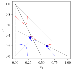
Figure 3: The figure shows the two degenerate stationary points in $\nu$-space that are mapped to a touching point of the inner triangle with of a fold line in $\alpha$-space under the catastrophe map $\chi_{\beta}$.

2.4.4 The elliptic umbilic temperature

We know from singularity theory that the elliptic umbilic is a doubly degenerate point, that is, a point where the Hessian has two zero eigenvalues. There is only one such point for this potential and it is given by $\beta=3$: The vanishing mixed second-order partial derivatives of the potential implies $\beta=\frac{1}{\nu_{3}}$. Plugging this into

$$\frac{\partial^{2}f_{\beta,\alpha}}{\partial\nu_{i}^{2}}=2\beta-\frac{1}{\nu_{i}}-\frac{1}{\nu_{3}}=0$$

yields $\frac{1}{\nu_{i}}=\beta$. These partial derivatives vanish therefore only for $\beta=3$ and $\nu=\frac{1}{3}(1,1,1)$ in zero magnetic field. Furthermore, the third-order Taylor expansion of the potential $f_{\beta,\alpha}$ for $\beta=3$ and zero magnetic field in the $(x,y)$-coordinates (34) is given by $-\frac{1}{3}y^{3}+x^{2}y+\mathrm{const}$. This is exactly the germ of the elliptic umbilic from Thom’s seven elementary catastrophes.

2.5 A parametric representation of the bifurcation set

As we have learned in the previous subsections, the extended phase diagram is constructed via the bifurcation set. In this subsection we present the parametric representation which was used to create Figure 1 and how it is obtained.

Theorem 8.

The bifurcation set is given by the union $F^{+}(\Delta^{2})\cup F^{-}(\Delta^{2})$ of the images of the two maps $F^{\pm}$ from $\Delta^{2}$ to the parameter space $(0,\infty)\times\Delta^{2}$ with components

$$F^{\pm}_{1}(\nu) =\frac{1}{3}\sum_{i=1}^{3}\frac{1}{\nu_{i}}\pm\sqrt{\frac{1}{9}\left(\sum_{i=1}^{3}\frac{1}{\nu_{i}}\right)^{2}-\frac{1}{3}\sum_{i<j}\frac{1}{\nu_{i}\nu_{j}}}$$ (47)

$$F^{\pm}_{2}(\nu) =\chi_{F_{1}^{\pm}(\nu)}(\nu)=\left(\frac{\nu_{i}e^{-F^{\pm}_{1}(\nu)\nu_{i}}}{\sum_{k=1}^{q}\nu_{k}e^{-F^{\pm}_{1}(\nu)\nu_{k}}}\right)_{i=1}^{3}$$ (48)

Proof.

First, let us check that $F^{+}$ and $F^{-}$ map $\Delta^{2}$ into $(0,\infty)\times\Delta^{2}$. Clearly, $F^{\pm}_{2}(\nu)$ is an element of $\Delta^{2}$. Furthermore, $F^{+}_{1}(\nu)$ is obviously positive. Since every $\nu_{i}$ is positive, we have

$$\sqrt{\frac{1}{9}\left(\sum_{i=1}^{3}\frac{1}{\nu_{i}}\right)^{2}-\frac{1}{3}\sum_{i<j}\frac{1}{\nu_{i}\nu_{j}}}<\frac{1}{3}\sum_{i=1}^{3}\frac{1}{\nu_{i}}$$ (49)

which implies that $F^{-}_{1}(\nu)$ is also positive. A point $(\beta,\alpha)$ belongs to the bifurcation set if and only there exists a degenerate stationary point $\nu$ in the unit simplex such that $\alpha=\chi_{\beta}(\nu)$. Lemma 3 shows us that the degeneracy condition (10) is a quadratic equation but this time considered as a function of $\beta$. Note also that it is independent of $\alpha$. The discriminant is given by

$$4(\nu_{1}\nu_{2}+\nu_{2}\nu_{3}+\nu_{3}\nu_{1})^{2}-12\nu_{1}\nu_{2}\nu_{3} =4((\nu_{1}\nu_{2}+\nu_{2}\nu_{3}+\nu_{3}\nu_{1})^{2}-3\nu_{1}\nu_{2}\nu_{3})$$ (50)

$$=4((\nu_{1}\nu_{2})^{2}+(\nu_{2}\nu_{3})^{2}-\nu_{1}\nu_{2}\nu_{3}+(\nu_{3}\nu_{1})^{2}).$$ (51)

On the boundary of the simplex, the discriminant is positive except at the vertices. We see by calculus that it achieves its minimal value at the centre of the simplex where it takes the value zero. Therefore the quadratic equation for $\beta$ has the two solutions $F^{\pm}_{1}(\nu)$ for every $\nu$.

Now that we know the two possible $\beta$-values that make $\nu$ fulfill the degeneracy condition we can use the catastrophe map $\chi_{\beta}$ to obtain the respective a-priori measures $\alpha$ to make them degenerate stationary points. This proves the claim. ∎

3 The stable phase diagram

The classical phase diagram is a partition of the parameter space. However, in contrast to the metastable phase diagram, the cells of this partition contain $(\beta,\alpha)$ such that the number of global minimizers stays constant inside the cell. This type of phase diagram does not see the fine bifurcation behaviour of the rate function and is therefore much simpler to describe. We can think of the classical phase diagram as given by a “surface” in the parameter space: the coexistence surface. On this surface we have a coexistence of at least two phases. It is therefore clear that the coexistence surface lies in those cells of the metastable phase diagram in which the rate function has at least two minimizers. The complement of the coexistence surface defines a region of the parameter space in which the rate function has a unique global minimum.

The surface is best understood by moving in the direction of increasing $\beta$ (see Figures 4, 5, 6 and 7). Leaving the high temperature regime ($\beta\leq 2$), it consists of three lines on the axis of symmetry. These lines have progeny, namely two lines emerging at a positive angle. This results in three Y-shaped sets composed of curved and straight lines. Furthermore, each of the offspring lines of the Y-shaped curves meet during the beak-to-beak scenario we have already seen in the extended phase diagram and form a triangle. Finally, the triangle shrinks to a point and we see a star-shaped set consisting of three straight lines (the axes of symmetry). On the coexistence surface the rate function has at least two and at most four global minimizers. The point of coexistence of four phases is the well-known Ellis-Wang point [7]. For $2<\beta\leq\frac{18}{7}$ it is only possible to have a coexistence of two phases. However, starting with $\beta$ larger than $\frac{18}{7}$ we find so-called triple points (coexistence of three phases). These will be important for our numerical computation of the Maxwell set (coexistence surface). Let us summarize our result:

Theorem 9.

Let us use the $(x,y)$-coordinates (34) for the $\alpha$-simplex.

1. For $\beta\leq 2$ the rate function has a unique global minimum for any $\alpha$.

2. For $2<\beta\leq\frac{18}{7}$ the rate function has precisely two global minimizers if $\alpha$ lies in the segment $\{0\}\times\left(-\frac{1}{2},-\frac{1-(\beta-2)e^{3-\beta}}{2+(\beta-2)e^{3-\beta}}\right)$ or its images under the permutation group. For any other $\alpha$ the rate function has a unique global minimum (see Figure 4).

3. For $\frac{18}{7}<\beta<4\log 2$ the rate function has precisely two global minimizers if $\alpha$ lies in the segment $\{0\}\times(-\frac{1}{2},y_{\mathrm{triple}}(\beta))$ or if $\alpha$ lies on the curve that is a solution to the initial value problem (59) or its images on the permutation group. Here, $y_{\mathrm{triple}}(\beta)$ is the $y$-coordinate of the triple point. If $\alpha$ is a triple point, the rate function has three global minimizers. For any other $\alpha$ it has a unique global minimum. (see Figures 5 and 6).

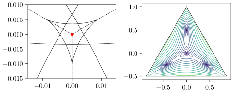
Figure 7: The left plot shows the Maxwell set (dashed lines) beyond Ellis-Wang together with the bifurcation set at the Ellis-Wang $\beta=4\log 2$. The Maxwell set looks the same at lower temperatures. The potential shows four equally deep minima for $\alpha$ at the red dot. Further decreasing the temperature, the central minimum will raise and eventually become a maximum.

4. For $\beta\geq 4\log 2$ the rate function has two global minimizers for any $\alpha$ on the segment $(-\frac{1}{2},0)\times\{0\}$ or its images under the permutation group. It has four global minimizers if $\beta=4\log 2$ and three global minimizers if $\beta>4\log 2$ for $\alpha=(\frac{1}{3},\frac{1}{3},\frac{1}{3})$. For any other $\alpha$ it has a unique global minimum (see Figure 7).

Now it is clear from the previous section that for $\beta\leq 2$ we do not see multiple global minimizers because points in the bifurcation set have $\beta>2$ and in a high temperature regime we have a unique global minimum. The other three regimes are interesting and it is useful to keep the bifurcation set in mind when analysing these. However, before we discuss the other regimes in detail let us state another observation which clarifies the word “surface” of the term coexistence surface: Locally (except at the triple points), this set is indeed a two-dimensional submanifold.

Suppose $(\beta,\alpha)$ is such that the rate function $f_{\beta,\alpha}$ has two distinct non-degenerate stationary points $\nu_{\beta,\alpha}$ and $\mu_{\beta,\alpha}$. Since the rate function depends smoothly on its parameters, the Implicit Function Theorem tells us that we find two smooth maps $(\beta,\alpha)\mapsto\nu_{\beta,\alpha}$ and $(\beta,\alpha)\mapsto\mu_{\beta,\alpha}$ that map a neighbourhood $U$ of $(\beta,\alpha)$ to $\Delta^{2}$ such that $\nu_{\beta,\alpha}$ and $\mu_{\beta,\alpha}$ are stationary points of $f_{\beta,\alpha}$ for every $(\beta,\alpha)$ in the neighbourhood.

Lemma 10.

The set of $(\beta,\alpha)$ such that $f_{\beta,\alpha}(\nu_{\beta,\alpha})=f_{\beta,\alpha}(\mu_{\beta,\alpha})$ is a two-dimensional embedded submanifold of $(0,\infty)\times\Delta^{2}$.

Proof.

Let us define the smooth map $F$ from $U$ to $\mathbb{R}$ via

$$F(\beta,\alpha)=f_{\beta,\alpha}(\nu_{\beta,\alpha})-f_{\beta,\alpha}(\mu_{\beta,\alpha}).$$ (52)

We now want to apply the Constant-Rank Level Set Theorem [23] for $F$ to conclude the proof. The differential of $F$ in terms of the $(\beta,u,v)$ coordinates is given via the row vector

$$\begin{pmatrix}-\frac{1}{2}(\|\nu_{\beta,\alpha}\|^{2}-\|\mu_{\beta,\alpha}\|^{2}),&(\mu_{\beta,\alpha})_{1}-(\nu_{\beta,\alpha})_{1},&(\mu_{\beta,\alpha})_{2}-(\nu_{\beta,\alpha})_{2}\end{pmatrix}$$ (53)

which is the zero map if and only if $\nu_{\beta,\alpha}=\mu_{\beta,\alpha}$. Thus, the differential has constant rank one. ∎

3.1 Coexistence in the regime of the rockets

In the regime of the rockets ($2<\beta\leq\frac{18}{7}$) the only cell that yields two local minimizers is given by the region enclosed by the rockets. The Maxwell set of this region is given by the intersection with the axes of symmetry. This is due to the fact that the two local minimizers lie in different fundamental cells of the simplex and that an asymmetry in the fields $\alpha$ leads to the same asymmetry in the global minimizer. This is explained by the following lemma which is inspired by Lemma 1 of [28].

Lemma 11 (Tilting Lemma).

Let $\nu$ be a global minimum of $f_{\beta,\alpha}$. If $\alpha_{i}>\alpha_{j}$, then $\nu_{i}>\nu_{j}$.

Proof.

Let $\nu^{\prime}_{j}=\nu_{i}$, $\nu^{\prime}_{i}=\nu_{j}$ and $\nu^{\prime}_{k}=\nu_{k}$ for $k$ not in $\{i,j\}$. Since

$$f_{\beta,\alpha}(\nu^{\prime})-f_{\beta,\alpha}(\nu)=(\nu_{i}-\nu_{j})(\log\alpha_{i}-\log\alpha_{j})\geq 0$$ (54)

and $\log\alpha_{i}-\log\alpha_{j}>0$, we conclude $\nu_{i}\geq\nu_{j}$. Assume $\nu_{i}=\nu_{j}$ and consider the push-forward of the tangent vector $v=\frac{\partial}{\partial\nu_{j}}-\frac{\partial}{\partial\nu_{i}}$:

$$df_{\beta,\alpha}(v)=\log\alpha_{i}-\log\alpha_{j}>0.$$ (55)

Thus $\nu$ is not a stationary point which contradicts the fact that $\nu$ is a minimizer. Therefore $\nu_{i}>\nu_{j}$. ∎

The cusp point of the rockets is given by the end point of the curve $\chi_{\beta}\circ\gamma_{\beta}(\nu_{1})$ which in this regime is $\nu_{1}=1-\frac{2}{\beta}$ (see Theorem 2). Thus the Maxwell set in $(x,y)$-coordinates is the segment

$$\{0\}\times\left(-\frac{1}{2},-\frac{1-(\beta-2)e^{3-\beta}}{2+(\beta-2)e^{3-\beta}}\right).$$ (56)

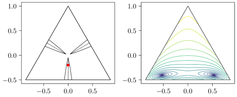
Figure 4: The left plot shows the Maxwell set (dashed lines) inside of the rockets. The right plot shows the contours of a typical point on the Maxwell set as indicated by the red dot in the left plot. The minimizers are equally deep and are mapped onto each other under reflection at the vertical axis.

3.2 Coexistence in the regime of disconnected pentagrams

In the regime $\frac{18}{7}<\beta<\frac{8}{3}$ three pentagrams have already unfolded but are still disconnected. As we have already discussed there are (modulo symmetry) three cells with two local minimizers and one cell with three local minimizers. The Maxwell set in cell I (see Figure 5) is the easiest. Here we have again two minimizers in different fundamental cells and therefore the Maxwell set is the intersection with the respective axis of symmetry. In the cells III and IV we also have two local minimizers but they lie in the same fundamental cell. Therefore the Tilting Lemma (Lemma 11) does not apply and the Maxwell set is a curved line deviating from the axis of symmetry. Cell II is special because we have three different local minimizers two of which lie in different fundamental cells. Since the classical phase diagram describes the degeneracy of the global minimum, we know that the Maxwell set continues on the axis of symmetry for as long as the two local minima from the different fundamental cells are lower than the third minimum. There exists however a point on the axis of symmetry at which this behaviour changes: the triple point. This is a point at which all minimizers are global minimizers. Since two of the local minimizers lie in different fundamental cells, the triple point must lie on the “star” (Lemma 11), that is, at least two components are equal. This is also the point where the Maxwell set leaves the axis of symmetry because the minimizers involved do not lie in different fundamental cells anymore. It suffices to compute the Maxwell set in either cell III or IV because of symmetry. The problem of computing the Maxwell set can be transformed into a solution of an initial value problem where the initial value is given by the triple point.

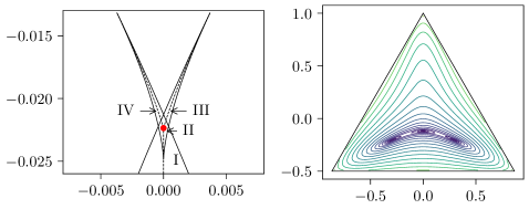
Figure 5: The left plot shows a magnification of one of the three pentagrams with its containing Maxwell set (dashed lines). The red dot marks the triple point at which all three minimizers are global minimizers. This can be seen in the right plot which shows a contour plot of the potential at the triple point.

Proposition 12.

For each positive $\beta$ there exists exactly one point $\alpha$ with $\alpha_{1}\leq\alpha_{2}\leq\alpha_{3}$ such that $f_{\beta,\alpha}$ has precisely three global minimizers.

Proof.

It is clear that the triple point $\alpha$ lies on the axis of symmetry. Therefore, let the curve $u\mapsto\alpha(u)$ be the axis of symmetry intersected with cell II. Then we have two local minimizers $\mu(u)$ and $\nu(u)$ of $f_{\beta,\alpha(u)}$ such that $\mu_{1}(u)>\nu_{1}(u)$. The difference

$$g(u):=f_{\beta,\alpha(u)}(\nu(u))-f_{\beta,\alpha(u)}(\mu(u))$$ (57)

is a monotonically increasing function of $u$:

$$g^{\prime}(u)=\frac{\partial f_{\beta,\alpha(u)}}{\partial u}=\mu_{1}(u)-\nu_{1}(u)>0.$$ (58)

∎

Proposition 13.

The set of all $\alpha$ such that the two local minimizers inside of the fundamental cell $\nu_{1}<\nu_{2}<\nu_{3}$ have the same depth is given in $(u,v)$-coordinates by the graph of $u\mapsto v(u)$ which is the solution of the initial value problem

$$\begin{split}\frac{dv}{du}&=-\frac{\nu_{1}(u,v)-\mu_{1}(u,v)}{\nu_{2}(u,v)-\mu_{2}(u,v)}\\ v(u_{0})&=v_{0}\end{split}$$ (59)

where $\alpha=(u_{0},v_{0})$ is the triple point, $\nu(u,v)$ and $\mu(u,v)$ are the two local minimizers of $f_{\beta,\alpha}$ in the same cell for $\alpha=(u,v(u))$.

Proof.

The curve fulfills

$$f_{\beta,\alpha(u)}(\nu(u,v))=f_{\beta,\alpha(u)}(\mu(u,v)).$$ (60)

Note that

$$\frac{d}{du}f_{\beta,\alpha(u)}(\nu(u,v))=\nu_{1}(u,v)-\nu_{2}(u,v)\frac{dv}{du}$$ (61)

since $\nu(u,v)$ is a stationary point. This proves the proposition. ∎

However, numerically computing the Maxwell set using this characterization is difficult because the mapping $u\mapsto(\nu(u,v),\mu(u,v))$ is not explicit. Therefore we consider the system of equations

$$f_{\beta,\alpha}(\mu) =f_{\beta,\alpha}(\nu)$$

$$\chi_{\beta}(\mu) =\chi_{\beta}(\nu)$$

instead. Because the free energy at a stationary point is given by

$$f_{\beta,\alpha}(\nu)=\sum_{i=1}^{3}\left(\frac{1}{2}\beta\nu_{i}^{2}+\nu_{i}\log\sum\limits_{j=1}^{3}\nu_{j}e^{-\beta\nu_{j}}\right)$$ (62)

this system does not depend on $\alpha$ and can be solved numerically for fixed values of $\beta$ and $\mu_{1}$. For better stability of the numerics we start with the triple point where the minimizers are well separated and then iteratively use the results as initial values for the next numerical step. In this way, the Figures 4, 5, 6 and 7 were obtained.

3.3 From beak-to-beak to Ellis-Wang

The qualitative nature of the Maxwell sets does not change with increasing $\beta$ after the beak-to-beak scenario until we reach the Ellis-Wang point. The cells with two minima which resulted from the merging of the horns of the pentagrams contain two minimizers which lie in the same fundamental cell as discussed in the previous subsection. Therefore the Maxwell set is again given by the solution to the initial value problem (59). This continues even after the crossing temperature where the central cell now contains four minima. Before the Ellis-Wang temperature the central fourth minimum is a local but not global minimum. The two outer minima each lie in the same fundamental cell so that the initial value problem applies. However, this changes after the Ellis-Wang point.

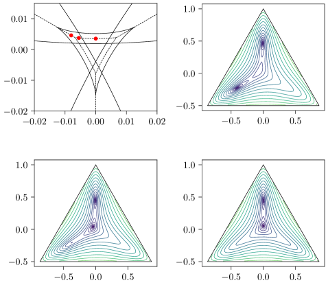
Figure 6: The upper left plot shows a magnification of the center of the simplex showing the bifurcation set together with the Maxwell set (dashed lines) for a $\beta$ between beak-to-beak and Ellis-Wang. Following the red dots on the Maxwell set from left to right we see how the potential changes in the upper right, lower left and lower right plots.

3.4 Beyond Ellis-Wang

At $\beta=4\log 2$ the outer minima and the central local minimum are equally deep. After the Ellis-Wang point ($\beta>4\log 2$), the outer minima are lower than the central minimum. They are equally deep in zero magnetic field and it is still possible using the Tilting Lemma to break the symmetry of the fields partially and achieve two equally deep minimizers. This can be done in the regime where the rate function has a local minimum in the centre ($\beta<3$) as well as in the regime where the local minimum has become a local maximum ($\beta>3$).

References

- [1] V.. Arnold, S.. Gusein-Zade and A.. Varchenko “Singularities of Differentiable Maps” Birkhäuser Boston, 1985 DOI: 10.1007/978-1-4612-5154-5
- [2] Anton Bovier and Frank Hollander “Metastability” In Grundlehren der mathematischen Wissenschaften Springer International Publishing, 2015 DOI: 10.1007/978-3-319-24777-9
- [3] Theodor Bröcker “Differentiable Germs and Catastrophes”, London Mathematical Society Lecture Note Series Cambridge University Press, 1975 DOI: 10.1017/CBO9781107325418
- [4] Raphaël Cerf and Matthias Gorny “A Curie–Weiss model of self-organized criticality” In The Annals of Probability 44.1 Institute of Mathematical Statistics, 2016, pp. 444–478 DOI: 10.1214/14-aop978
- [5] Sourav Chatterjee and Qi-Man Shao “Nonnormal Approximation By Stein’s Method of Exchangeable Pairs With Application To the Curie-Weiss Model” In The Annals of Applied Probability 21.2, 2011, pp. 464–483 DOI: 10.1214/10-aap712
- [6] Peter Eichelsbacher and Bastian Martschink “On rates of convergence in the Curie–Weiss–Potts model with an external field” In Annales de l’Institut Henri Poincaré, Probabilités et Statistiques 51.1 Institute of Mathematical Statistics, 2015, pp. 252–282 DOI: 10.1214/14-aihp599
- [7] Richard S. Ellis and Kongming Wang “Limit theorems for the empirical vector of the Curie-Weiss-Potts model.” In Stochastic Processes Appl. 35.1 Elsevier (North-Holland), Amsterdam, 1990, pp. 59–79 DOI: 10.1016/0304-4149(90)90122-9
- [8] A… Enter, R. Fernández, F. den Hollander and F. Redig “Possible loss and recovery of Gibbsianness during the stochastic evolution of Gibbs measures.” In Commun. Math. Phys. 226.1 Springer, Berlin/Heidelberg, 2002, pp. 101–130 DOI: 10.1007/s002200200605
- [9] Aernout C.. Enter, Victor N. Ermolaev, Giulio Iacobelli and Christof Külske “Gibbs–non-Gibbs properties for evolving Ising models on trees” In Annales de l’Institut Henri Poincaré, Probabilités et Statistiques 48.3 Institute of Mathematical Statistics, 2012, pp. 774–791 DOI: 10.1214/11-aihp421
- [10] Aernout C.. Enter, Christof Külske, Alex A. Opoku and Wioletta M. Ruszel “Gibbs–non-Gibbs properties for n-vector lattice and mean-field models” In Brazilian Journal of Probability and Statistics 24.2 Institute of Mathematical Statistics, 2010, pp. 226–255 DOI: 10.1214/09-bjps029
- [11] R. Fernández, F. Hollander and J. Martínez “Variational Description of Gibbs-non-Gibbs Dynamical Transitions for the Curie-Weiss Model” In Communications in Mathematical Physics 319.3 Springer ScienceBusiness Media LLC, 2012, pp. 703–730 DOI: 10.1007/s00220-012-1646-1
- [12] J. Gaite, J. Margalef-Roig and S. Miret-Artés “Analysis of a Three-Component Model Phase Diagram By Catastrophe Theory” In Physical Review B 57.21, 1998, pp. 13527–13534 DOI: 10.1103/physrevb.57.13527
- [13] J. Gaite, J. Margalef-Roig and S. Miret-Artés “Analysis of a Three-Component Model Phase Diagram By Catastrophe Theory: Potentials With Two Order Parameters” In Physical Review B 59.13, 1999, pp. 8593–8601 DOI: 10.1103/physrevb.59.8593
- [14] J.. Gaite “Phase Transitions As Catastrophes: The Tricritical Point” In Physical Review A 41.10, 1990, pp. 5320–5324 DOI: 10.1103/physreva.41.5320
- [15] Reza Gheissari, Charles M. Newman and Daniel L. Stein “Zero-Temperature Dynamics in the Dilute Curie–Weiss Model” In Journal of Statistical Physics 172.4 Springer ScienceBusiness Media LLC, 2018, pp. 1009–1028 DOI: 10.1007/s10955-018-2087-9
- [16] F. Hollander, F. Redig and W. Zuijlen “Gibbs-Non-Gibbs Dynamical Transitions for Mean-Field Interacting Brownian Motions” In Stochastic Processes and their Applications 125.1, 2015, pp. 371–400 DOI: 10.1016/j.spa.2014.09.011
- [17] Benedikt Jahnel and Christof Külske “The Widom–Rowlinson model under spin flip: Immediate loss and sharp recovery of quasilocality” In The Annals of Applied Probability 27.6 Institute of Mathematical Statistics, 2017, pp. 3845–3892 DOI: 10.1214/17-aap1298
- [18] Sascha Kissel and Christof Külske “Dynamical Gibbs-non-Gibbs transitions in Curie-Weiss Widom-Rowlinson models” In Markov Processes Relat. Fields 25, 2019, pp. 379–413
- [19] Sascha Kissel and Christof Külske “Dynamical Gibbs–Non-Gibbs Transitions in Lattice Widom–Rowlinson Models with Hard-Core and Soft-Core Interactions” In Journal of Statistical Physics Springer ScienceBusiness Media LLC, 2020 DOI: 10.1007/s10955-019-02478-y
- [20] Richard C. Kraaij, Frank Redig and Willem B. Zuijlen “A Hamilton-Jacobi point of view on mean-field Gibbs-non-Gibbs transitions”, 2017 arXiv:1711.03489v1
- [21] Christof Külske and Arnaud Le Ny “Spin-flip dynamics of the Curie-Weiss model: loss of Gibbsianness with possibly broken symmetry.” In Commun. Math. Phys. 271.2 Springer, Berlin/Heidelberg, 2007, pp. 431–454 DOI: 10.1007/s00220-007-0201-y
- [22] C. Landim and I. Seo “Metastability of Non-Reversible, Mean-Field Potts Model With Three Spins” In Journal of Statistical Physics 165.4, 2016, pp. 693–726 DOI: 10.1007/s10955-016-1638-1
- [23] John M. Lee “Introduction to Smooth Manifolds” In Graduate Texts in Mathematics Springer New York, 2012 DOI: 10.1007/978-1-4419-9982-5
- [24] Yung-Chen Lu “Introduction to Singularity Theory with Historical Remarks” In Singularity Theory and an Introduction to Catastrophe Theory New York, NY: Springer New York, 1976, pp. 1–23 DOI: 10.1007/978-1-4612-9909-7_1
- [25] Enzo Olivieri and Maria Eulália Vares “Large Deviations and Metastability” Cambridge University Press, 2005 DOI: 10.1017/cbo9780511543272
- [26] Tim Poston and Ian Stewart “Catastrophe Theory and its Applications” London etc.: Pitman Publishing Ltd., 1978
- [27] Mira Shamis and Ofer Zeitouni “The Curie-Weiss Model With Complex Temperature: Phase Transitions” In Journal of Statistical Physics 172.2, 2017, pp. 569–591 DOI: 10.1007/s10955-017-1812-0
- [28] Kongming Wang “Solutions of the Variational Problem in the Curie-Weiss-Potts Model” In Stochastic Processes and their Applications 50.2, 1994, pp. 245–252 DOI: 10.1016/0304-4149(94)90121-x
- [29] F.. Wu “The Potts Model” In Reviews of Modern Physics 54.1, 1982, pp. 235–268 DOI: 10.1103/revmodphys.54.235