A 3D view of the Taurus star-forming region by Gaia and Herschel:

Abstract

Context. Taurus represents an ideal region to study the three-dimensional distribution of the young stellar population and relate it to the associated molecular cloud.

Aims. The second Gaia data release (DR2) enables us to investigate the Taurus complex in three dimensions, starting from a previously defined robust membership. The molecular cloud structured in filaments can be traced in emission using the public far-infrared maps from Herschel.

Methods. From a compiled catalog of spectroscopically confirmed members, we analyze the 283 sources with reliable parallax and proper motions in the Gaia DR2 archive. We fit the distribution of parallaxes and proper motions with multiple populations described by multivariate Gaussians. We compute the cartesian Galactic coordinates (X,Y,Z) and, for the populations associated with the main cloud, also the galactic space velocity (U,V,W). We discuss the spatial distribution of the populations in relation to the structure of the filamentary molecular cloud traced by Herschel.

Results. We discover the presence of six populations which are all well defined in parallax and proper motions, with the only exception being Taurus D. The derived distances range between $\sim$130 and $\sim$160 pc. We do not find a unique relation between stellar population and the associated molecular cloud: while the stellar population seems to be on the cloud surface, both lying at similar distances, this is not the case when the molecular cloud is structured in filaments. Taurus B is probably moving in the direction of Taurus A, while Taurus E appears to be moving towards them.

Conclusions. The Taurus region is the result of a complex star formation history which most probably occurred in clumpy and filamentary structures that are evolving independently.

1 Introduction

During the early phases of the star and cluster formation process, filamentary structures have not only been theoretically predicted (e.g., Dale et al. 2012), but have also been detected in low- and high-mass star-forming regions, and in regions where no star formation is currently active (e.g., André et al. 2010). In particular, Myers (2009) highlights that near young stellar groups or clusters are associated with a “hub-filament structure”. Filaments traced commonly by extinction maps from infrared observations can now be traced in great detail in emission in the far-infrared thanks to Herschel. Within 300 pc we find examples of a main prominent filament in Chamaeleon I or Corona Australis (e.g., Schmalzl et al. 2010; Palmeirim et al. 2013; Sicilia-Aguilar et al. 2011, 2013); Lupus I is instead located along a filament at the converging location of two bubbles (e.g., Gaczkowski et al. 2015, 2017; Krause et al. 2018), while Serpens Main is at the converging point of filaments (e.g., Roccatagliata et al. 2015).
A step further in the study of filamentary molecular clouds is to relate their physical properties to young stellar populations. This can be done by combining the astrometric Gaia data with the Herschel maps of the molecular cloud in emission. The second release of Gaia is revolutionizing the study of star formation and young clusters under different aspects. A 3D density map for early-type and pre-main sequence sources was recently constructed by, for example, Zari et al. (2018), finding that younger stars within 500 pc to the Sun are mostly distributed in dense and compact clumps, while older sources are instead widely distributed. Several studies on large-scale star-forming regions are combining Gaia data with photometric surveys (e.g., Vela OB2, Armstrong et al. 2018; Cantat-Gaudin et al. 2018). New members have been found in nearby associations (e.g., Gagné & Faherty 2018), and even new nearby associations have been discovered (e.g., Gagné et al. 2018). Recently, multiple populations were also detected in young clusters (Roccatagliata et al. 2018; Franciosini et al. 2018).
One of the most studied young star forming regions, where both a prominent molecular cloud is structured in a main filament and a young population is present, is the Taurus complex. The discussion of star formation history in space and time started more than 15 years ago. Palla & Stahler (2002) found a younger population inside the filaments and a more dispersed and older population outside them, and concluded that an age spread was present in the region. In the same year, overlaying the young stellar content to the ¹²CO maps, Hartmann (2002) found that most of the sources in “Taurus Main” follow three near parallel elongated bands, while only a few of them are localized in widely distributed groups. This led him to organize the sources into different groups according to their spatial distribution, without finding a significant age spread in the K7-M1 spectral type range. Continuum and line maps of the region with increasing spatial resolution have been obtained for Taurus in recent years. A large-scale survey of Taurus in ¹²CO and ¹³CO was presented by Goldsmith et al. (2008), showing a very complex and highly structured cloud morphology including filaments, cavities, and rings. Analyzing the ¹³CO integrated intensities in three different velocity intervals, these latter authors found the highest velocity (7-9 km/s) corresponding to L1506 and L1498 and part of L1495, while the other clouds (B213, L1521, B18, L1536) have mainly intermediate velocities (5-7 km/s) and only a few points at the borders of those clouds are found at even lower velocities (3-5 km/s). A different orientation of the magnetic field was also found: the long filament of L1506 is parallel to the field, while the magnetic field is perpendicular to the extension of the long axis of the B216 and B217 filaments (Goodman et al. 1992).
The main filament in the B213-L1495 region has been extensively studied by Hacar et al. (2013) in high-density tracers such as C¹⁸O, N₂H⁺, and SO, and by Hacar et al. (2016) in the three main isotopologs of ¹²CO, ¹³CO, and C¹⁸O. These latter authors suggested that the velocity broadening of the lines could be caused by the effects of different structures in 3D, which are clumpy or tangly on the line of sight projection of the velocity component.

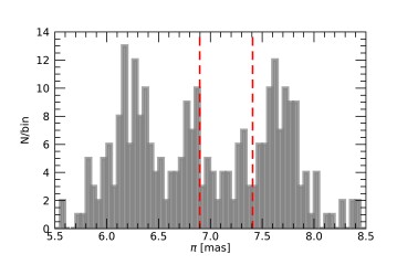
Figure 1: Histogram of the parallaxes of the Taurus members. The dashed red lines indicate the range in parallax commonly adopted in the literature.

A first analysis of the Gaia DR2 data of Taurus recently presented by Luhman (2018) and Esplin & Luhman (2019) enabled these authors to revise the membership and to constrain the initial mass function of Taurus. Using the Gaia data, Luhman (2018) found that the population older that 10 Myr is not associated to Taurus.

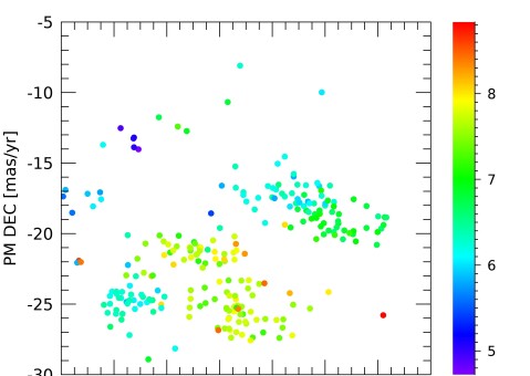
Figure 2: Proper motions in $\alpha$ and $\delta$ color coded by the parallax of the sources.

The goal of the present paper is to relate the star formation history in the Taurus complex to the filamentary structure of the molecular cloud. To this aim, the new analysis of the Gaia DR2 data starts from a reliable membership (presented in Sect. 2) and applies a rigorous approach which takes into account the covariances (not considered in the studies of Luhman 2018; Esplin & Luhman 2019) between parallax and proper motions (available in the Gaia Archive). The cluster kinematics and the relation between stellar content and filamentary structures are discussed in Sect. 4, together with the estimate of the distance of the molecular cloud. Our conclusions are presented in Sect. 5.

2 Cluster membership and Gaia DR2 data

Of the initial catalog of 518 spectroscopically confirmed members of Esplin & Luhman (2019), 443 sources are present in the Gaia DR2 archive. From this sample, we selected the sources with good astrometry following Lindegren (2018), who suggested the use of renormalized unit weight error (RUWE), which is a more reliable and informative goodness-of-fit statistic than the astrometric excess noise commonly used until now by the community. The RUWE is defined as

$$RUWE=\frac{\sqrt{\chi^{2}/(nObs-\nu)}}{f(G,G_{BP}-G_{RP})},$$ (1)

where $nObs$ is the number of observations, $\nu$ is the number of parameters solved, and $f$ is a renormalization function. Our further analysis is based on the 283 sources with RUWE of less than 1.4.
Figure 1 shows the distribution of the parallaxes of the cluster members. The resulting mean parallax is 7.01$\pm$0.06 mas, where the associated error is computed as the standard deviation (0.78 mas) divided by $\sqrt{N}$. However, this mean parallax value lies exactly in the middle of a parallax distribution that appears to be multimodal. Furthermore, the distribution in proper motions in Fig. 2 shows that multiple populations might be present in the region. A deeper analysis of the Gaia data is therefore necessary to understand the star formation history of the region.

3 Analysis

Figures 1 and 2 clearly show that Taurus cannot be described by a single population because both parallaxes and proper motions are not randomly distributed around single mean values. Therefore, we model the distribution of the astrometric parameters using a similar approach to that used by Roccatagliata et al. (2018) to study the two sub-populations in Chamaeleon I. We assume that the Taurus star forming region is composed of multiple populations, each described by a 3D multivariate Gaussian (as in Lindegren et al. 2000, ). The $j$-th population is defined by seven parameters: the mean parallax ($\pi_{j}$), the mean proper motions along right ascension and declination ($\mu_{\alpha,j}$ and $\mu_{\delta,j}$), the intrinsic dispersion of the parallax ($\sigma_{\pi,j}$), the intrinsic dispersion of proper motions along right ascension and declination($\sigma_{\mu_{\alpha},j}$ and $\sigma_{\mu_{\delta},j}$), and a normalization factor that takes into account the fraction of stars belonging to that population ($f_{j}$). We assume that the mean proper motions and the mean parallaxes of each population are not correlated. To fit our distribution we use a maximum likelihood technique as in Jeffries et al. (2014) and Franciosini et al. (2018), adopting the slsqp minimization method as implemented in scipy. The likelihood function of the $i$-th star for the $j$-th population is given by

$$L_{i,j}=(2\pi)^{-3/2}\,|C_{i,j}|^{-1/2}\times\exp{\begin{bmatrix}-\frac{1}{2}(a_{i}-a_{j})^{\prime}\,C_{i,j}^{-1}\,(a_{j}-a_{i})\end{bmatrix}},$$ (2)

where $C_{i,j}$ is the covariance matrix, $|C_{i,j}|$ its determinant, and
$(a_{i}-a_{j},)^{\prime}$ is the transpose of the vector

$$a_{i}-a_{j}=\begin{bmatrix}\pi_{i}-\pi_{j},\\ \mu_{\alpha,i}-\mu_{\alpha,j}\\ \mu_{\delta,i}-\mu_{\delta,j}\end{bmatrix}.$$ (3)

Following Lindegren et al. (2000), the covariance matrix $C_{i,j}$ is given by:

$$\small C_{i}\,=\,\begin{bmatrix}\sigma_{\pi,i}^{2}+\sigma_{\pi,j}^{2}&\sigma_{\pi,i}\,\sigma_{\mu_{\alpha,i}}\,\rho_{i}\,(\pi,\mu_{\alpha})&\sigma_{\pi,i}\,\sigma_{\mu_{\delta,i}}\,\rho_{i}\,(\pi,\mu_{\delta})\\ \sigma_{\pi,i}\,\sigma_{\mu_{\alpha,i}}\,\rho_{i}\,(\pi,\mu_{\alpha})&\sigma_{\mu_{\alpha,i}}^{2}+\sigma_{\mu_{\alpha,j}}^{2}&\sigma_{\mu_{\alpha,i}}\,\sigma_{\mu_{\delta,i}}\cdot\rho_{i}\,(\mu_{\alpha},\mu_{\delta})\\ \sigma_{\pi,i}\,\sigma_{\mu_{\delta,i}}\,\rho_{i}\,(\pi,\mu_{\delta})&\sigma_{\mu_{\alpha,i}}\,\sigma_{\mu_{\delta,i}}\,\rho_{i}\,(\mu_{\alpha},\mu_{\delta})&\sigma_{\mu_{\delta,i}}^{2}+\sigma_{\mu_{\delta,j}}^{2}\end{bmatrix},$$ (4)

where $\rho_{i}\,(\pi,\mu_{\alpha})$, $\rho_{i}\,(\pi,\mu_{\delta})$, $\rho_{i}\,(\mu_{\alpha},\mu_{\alpha})$ are the non-diagonal elements of the covariance matrix of each star provided by the Gaia archive.

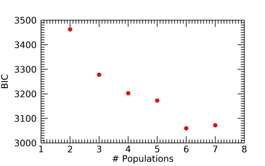
Figure 3: Values of the BIC calculated for the fits with different numbers $n$ of populations.

The total likelihood for the $i$-th star is given by:

$$L_{i}=\sum_{j=1}^{n}f_{j}\,L_{i,j},$$ (5)

where $n$ is the number of populations and $\sum_{j=1}^{n}f_{j}=1$. The probability for each star of belonging to the $j$-th population is then

$$\vskip 3.0pt plus 1.0pt minus 1.0ptP_{i,j}\,=\,f_{j}\,\frac{L_{i,j}}{L_{i}}.$$ (6)

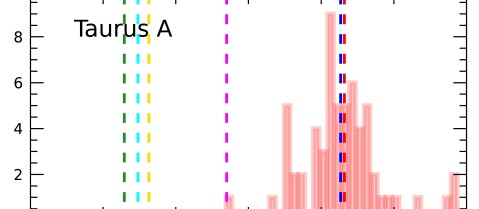
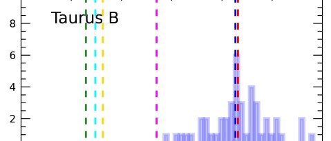
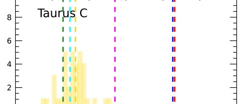
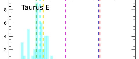
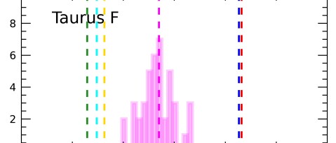
Figure 4: Parallax distribution of the most probable members (P$\geq$80$\%$) of the Taurus A (red), Taurus B (blue), Taurus C (yellow), Taurus D (green), Taurus E (cyan), and Taurus F (magenta) populations. In each panel the maximum-likelihood parallaxes for the six populations are also shown as vertical dashed lines using the color code of the histograms.

We fitted our data with a series of models, starting with two populations, and adding one population at a time. We note that each additional population requires that seven new free parameters be fitted (the three centroids of parallax and proper motions and the relative dispersions, plus the fraction of stars). The statistical significance of each model was tested using the Bayesian information criterion (BIC), which takes into account both the maximum-likelihood and the number of free parameters of the model in order to reduce the risk of overfitting. The resulting values are shown in Fig. 3: we see that the BIC decreases up to six populations and then starts to increase again. Therefore, we conclude that the model with six populations is the best fit of our data, given our assumptions. The best fit parameters for the six populations, which we call Taurus A, B, C, D, E and F, are listed in Table 1, while the probability of each star belonging to each population is reported in Table 3. Between the six probabilities for each source, the highest identifies the population with which that source is associated. We find that 253 of the 283 stars used for the calculations have a probability of higher than 80% of belonging to one of the six populations: 62 to Taurus A, 46 to Taurus B, 36 to Taurus C, 27 to Taurus D, 40 to Taurus E, and 42 to Taurus F. The distribution of parallaxes and proper motions of these 253 stars are shown in Figs. 4 and 5, respectively. In Fig. 6 (see Sect. 4.2) we show their spatial distribution relative to the molecular cloud traced by Herschel far-infrared images.
We note that the majority of the members of the six populations that have been selected using only proper motions and parallaxes are also well separated in the plane of the sky. This is independent confirmation of the results of our analysis.

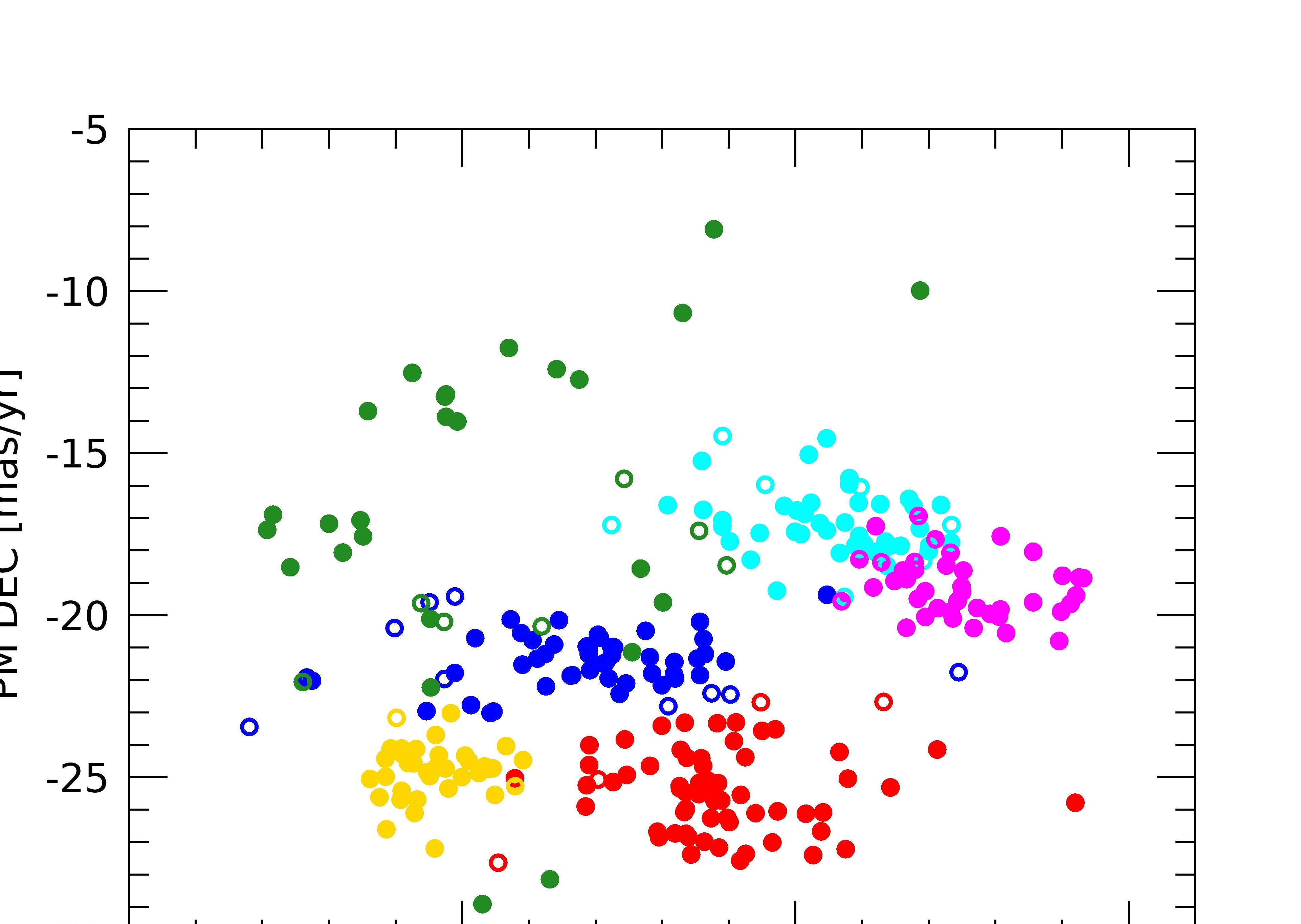
Figure 5: Proper motions in $\alpha$ and $\delta$ of the six populations, color coded as in Fig. 4. The filled dots represent sources with probabilities higher than 80%, while the empty circles represent sources with probabilities lower than 80%.

The relative errors on the derived parallaxes are of the order of 1% or less, and therefore the bias to the distance calculated by inverting the parallaxes is negligible (Luri et al. 2018; Bailer-Jones 2015). We find that three of the populations are associated with Taurus Main: Taurus A and B, located at similar distances (130.5${}^{+0.5}_{-0.5}$ pc and 131.0${}^{+1.0}_{-1.0}$ pc, respectively), and Taurus E further away at a distance of 160.3${}^{+0.6}_{-0.6}$ pc. Taurus C and F are located in the clouds outside Taurus Main, at 158.4${}^{+0.6}_{-0.6}$ pc and 146.0${}^{+0.6}_{-0.6}$ pc, respectively. With a mean distance of 162.7${}^{+4.4}_{-4.1}$ pc, Taurus D is the least defined population, with a large spread both in astrometric parameters and in the spatial distribution.
All the given errors in the parallaxes and distances include only the statistical uncertainties from the fit. At these distances, the conservative systematic error of 0.1 mas discussed by Luri et al. (2018) corresponds to $\sim\,$2 pc.

Table 1: Results from the maximum-likelihood fit for the parallaxes and proper motions, and relative dispersions, of Taurus A, B, C, D, E and F. In the last line we report the distance in parsecs of the six populations computed as described in the text.

	Taurus A	Taurus B	Taurus C	Taurus D	Taurus E	Taurus F
$\pi$ [mas]	7.660 $\pm$ 0.029	7.634 $\pm$ 0.058	6.314 $\pm$ 0.025	6.145 $\pm$ 0.161	6.240 $\pm$ 0.024	6.850 $\pm$ 0.029
$\mu_{\alpha}$ [mas/yr]	8.780 $\pm$ 0.144	6.883 $\pm$ 0.258	4.618 $\pm$0.108	5.572 $\pm$ 0.454	10.490 $\pm$0.209	12.413 $\pm$ 0.167
$\mu_{\delta}$ [mas/yr]	$-$25.373 $\pm$ 0.201	$-$21.380 $\pm$ 0.170	$-$24.842 $\pm$ 0.138	$-$17.368 $\pm$ 0.934	$-$17.172 $\pm$ 0.168	$-$19.077 $\pm$ 0.145
$\sigma_{\pi,0}$ [mas]	0.192 $\pm$ 0.025	0.271 $\pm$ 0.058	0.101 $\pm$ 0.027	0.663 $\pm$ 0.101	0.088 $\pm$ 0.034	0.136 $\pm$ 0.024
$\sigma_{\mu_{\alpha},0}$ [mas/yr]	1.073 $\pm$ 0.113	1.358 $\pm$ 0.174	0.591 $\pm$ 0.079	2.298 $\pm$ 0.314	1.141 $\pm$ 0.164	0.976 $\pm$ 0.147
$\sigma_{\mu_{\delta,0}}$ [mas/yr]	1.268 $\pm$ 0.159	0.847 $\pm$ 0.123	0.770 $\pm$ 0.109	4.738 $\pm$ 0.612	1.006 $\pm$ 0.126	0.891 $\pm$ 0.103
$f$	0.233 $\pm$ 0.027	0.189 $\pm$ 0.028	0.129 $\pm$ 0.021	0.127 $\pm$ 0.027	0.163 $\pm$ 0.024	0.159 $\pm$ 0.057
d [pc]	130.5${}^{+0.5}_{-0.5}$	131.0${}^{+1.0}_{-1.0}$	158.4${}^{+0.6}_{-0.6}$	162.7${}^{+4.4}_{-4.1}$	160.3${}^{+0.6}_{-0.6}$	146.0${}^{+0.6}_{-0.6}$

4 Discussion

We organize the discussion as follows. First we compare the distances of the six populations to the literature values. We then investigate the properties and distance of the molecular cloud in order to be able to relate the 3D distribution of the stellar population to the molecular cloud.

4.1 Distances of the Taurus stellar populations

The distance of the Taurus complex reported in the literature (e.g., Preibisch & Smith 1997) and commonly used so far is consistent with the average parallax of 7.01 mas that we found previously, but this can no longer be considered valid in light of the present results, which show different distances for the six populations, ranging from 130 pc for Taurus A to 160 pc for Taurus C.
Several measurements at different wavelengths and using different methods have been taken in recent decades to investigate the distance of the Taurus complex. Accurate distances derived from VLBI astrometry are available for several stars. Values of 128.5$\pm$0.6 pc, 132.8$\pm$0.5 pc, and 132.8$\pm$2.3 pc were found for Hubble 4, HDE 283572, and the binary V773 Tau, respectively (Torres et al. 2007, 2012), while a distance of 161.2$\pm$0.9 pc was found for the HPTau/G2 system (Torres et al. 2009). Galli et al. (2018) derived VLBI distances for an additional 18 Taurus members, finding values ranging from 84 to 162 pc. We note also that Kenyon et al. (1994) already suggested that the canonical distance of 140$\pm$10 pc was not representative of most stars in this region since they measured a significant depth effect using optical spectrophotometry of field stars projected on the molecular cloud. On the contrary, Dzib et al. (2018), using the Gaia data alone, found that L1495 in Taurus lies at 129 pc, which corresponds to the distance of Taurus A in our analysis.
The presence of multiple populations was also investigated by a recent study of Luhman (2018), who used colors to identify different populations; we report those colours in Table 3. We find that all the stars that we classify as part of Taurus A and Taurus B belong to the red population of Luhman (2018), while stars in Taurus C belong to his cyan population. The blue population corresponds to Taurus E and F, while Taurus D includes sources from all the populations found by Luhman (2018). This is to be expected since this is the most spatially dispersed population, without a clear peak in the parallax distribution. We conclude that the populations found by Luhman (2018) are only partially consistent with ours. This is because we adopted completely different approaches. In his case, starting from the spatial distribution of sources in correspondence to the different clouds, Luhman (2018) characterized their average parallax and proper motions without any additional statistical analysis able to take into account the errors and correlations between astrometric parameters. Recently, Galli et al. (2019) also studied the Taurus populations, instead applying a hierarchical clustering algorithm and removing the outliers using the minimum covariance determinant. These latter authors found 21 clusters, which are also indicated in Table 3, most of which, however, have less than eight members. To compare this latter result with the four populations found by Luhman (2018), Galli et al. (2019) defined six groups of clusters, which are consistent with the four populations of Luhman (2018). Comparing our results with the group classification of Galli et al. (2019), we find that Taurus A and B, both red in Luhman (2018), correspond to Group F in Galli et al. (2019), that Taurus C corresponds to Group C (cyan in Luhman 2018), Taurus E mostly corresponds to Group A, and Taurus F corresponds to Group B (both blue in Luhman 2018).

It is important to highlight the fact that our decision to not start our analysis from the spatial distribution of the sources (as is highly recommended in clusters without a centrally peaked spatial distribution) is motivated by the fact that we wanted to investigate whether or not the molecular cloud, which is mainly structured in filaments, is shaping the spatial distribution of the different populations.

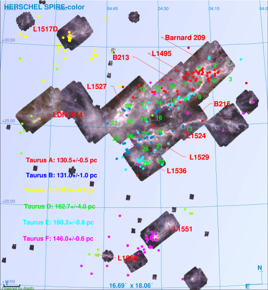
Figure 6: Herschel RGB color composition using all public SPIRE observations from the Herschel Science Archive at 250 $\mu$m (blue), 350 $\mu$m (green), and 500 $\mu$m (red). The filled circles represent the most probable members of Taurus A (in red), Taurus B (in blue), Taurus C (in yellow), Taurus D (in green), Taurus E (in cyan) and Taurus F (in magenta). With Taurus Main we refer to the Taurus complex excluding the clouds L1517D, LDN 1551 and L1558. The green numbers which appear only on Taurus Main correspond to the distances in parsec computed in those positions by Zucker et al. (2019). In red we indicate the names of the clouds in the region. At 150 pc the size of 1^∘ corresponds to 2.6 pc.

4.2 Taurus molecular clouds and stellar populations

We can now begin to discuss the Taurus star formation history by combining the new Gaia results with high-resolution observations of the filaments in Taurus from Herschel. A similar approach was used by Großschedl et al. (2018) with Orion A finding that this is a cometary-like cloud and that the straight filamentary cloud is only its projection.
A large-scale continuum map of the Taurus complex was computed from the near-infrared extinction map from Schmalzl et al. (2010). The Herschel observations of Taurus were obtained in the context of the Gould Belt survey (Kirk et al. 2013; Palmeirim et al. 2013) allowing point-source extraction and the determination of the temperature and density profile of the main filament in the LDN 1495 region. Figure 6 shows a composite Herschel map of the Taurus complex combining all the public SPIRE observations available in the archive . The positions of the Taurus A, B, C, D, E and F populations are also shown, as well as the position of the known clouds in the region. We find that, in the Taurus Main cloud, Taurus A and B are at a similar distance, while Taurus E is located 30 pc further away. The greatest concentration of sources of Taurus A spreads over the B209 cloud. In the rest of Taurus Main, all populations follow the filamentary structure traced by the Herschel maps. Taurus B, in particular, is mostly distributed along the L1524 and L1529 clouds, while Taurus E is projected in the direction of the filamentary clouds L1495 and B213 and on the cloud L1536. The bulk of the population of Taurus C corresponds to the L1517 cloud, while Taurus F is concentrated on L1551. Few sources of Taurus D are close to the L1544 and L1558 clouds, but in general this population is distributed over the entire complex. A possible explanation for this behavior, given also the spread in parallax and proper motions, is that Taurus D is not a single population but the combination of multiple substructures, which our analysis is not able to distinguish; it may also represent a dispersed young population.

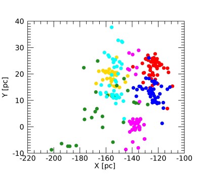
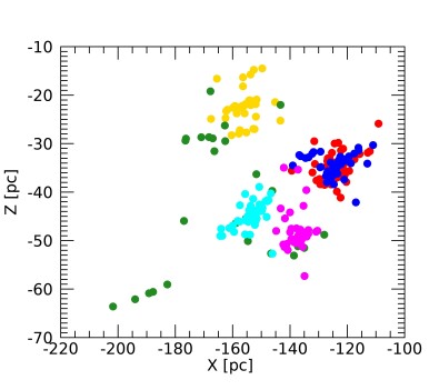
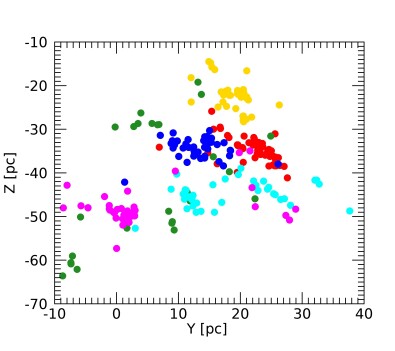
Figure 7: Two-dimensional projections of the 3D spatial distribution of the multiple populations of Fig. 9 . The color code is as in Fig. 4.

Figure 9 shows the 3D spatial distribution of the six populations in cartesian galactic coordinates (X,Y,Z), where the X axis points towards the galactic center, Y towards the local direction of rotation in the plane of the galaxy, and Z towards the North Galactic Pole. In particular, given the galactic coordinates $(l,b)$, X,Y,Z are defined as:

$$\begin{array}[]{l}X=d\,\cos\,b\,\cos\,l\\ Y=d\,\sin\,l\,\cos\,b\\ Z=d\,\sin\,b.\end{array}$$ (7)

The projection of the 3D distribution of the six populations on the individual planes is shown in Fig. 7. We find that Taurus A and B in the (X,Z) projection are compact and overlapped, while in the other two projections they are separated but close; both populations extend for about 20 pc along the X axis and 10 pc along the Y and Z axes. In the (X,Y) and (X,Z) planes, Taurus C is distributed along three parallel lines separated by a few parsecs and extending for about 10 pc. In the (Y,Z) projection, this population has a more compact structure in the center, which is slightly elongated by about 5 pc in the Y direction. Taurus D is also confirmed to be a spread population in 3D. Taurus E has a compact structure of 20$\times$10 pc only in the (X,Z) plane; in the other two projections, it shows a compact structure of 20$\times$5 pc and 5$\times$10 pc in the (X,Y) and (Y,Z) planes, respectively, which corresponds to the L1536 cloud. This structure is connected by a few sources along 10 pc to a linear distribution of sources of 10 pc in length corresponding to the L1495 filament. The bulk of sources of Taurus F are concentrated within 10 pc in X and 5 pc in Y and Z; this corresponds to the L1551 cloud. A few additional sources are scattered over 20 pc in X and Z, and $\sim$40 pc in Y.
The distance of the molecular cloud can be estimated using the field stars in and outside of the cloud from Gaia DR2. This was done recently by Yan et al. (2019), who found a single distance of 145${}^{+12}_{-16}$ pc for the entire molecular cloud. A similar approach was adopted by Zucker et al. (2019), who compiled a uniform catalog of distances to local molecular clouds. The methodology of these latter authors, based on the work of Schlafly et al. (2014), infers a joint probability distribution function on distance and reddening for individual stars based on optical and near-infrared photometric surveys and Gaia parallaxes, and also on modeling of the cloud as a simple dust screen to bracket the dust screen between unreddened foreground stars and reddened background stars. The work of Zucker et al. (2019) allowed the authors to not only find a single distance for the surface of the Taurus molecular cloud of 141$\pm$9 pc, but also to map the 3D surface of the region previously defined as Taurus Main.

Table 2: Local distances in Taurus Main computed by Zucker et al. (2019) with: the number appearing in Fig. 6 (col.1 & 4), galactic positions (col.2 & 5), and the distances (col.3 & 6).

#	l [∘] , b [∘]	D [pc]	#	l [∘] , b [∘]	D [pc]
1	167.3, -16.3	133${}^{+3}_{-2}$	16	173.0, -15.1	139${}^{+16}_{-14}$
2	168.0, -15.7	116${}^{+17}_{-15}$	17	173.0, -13.9	127${}^{+5}_{-4}$
3	168.0, -17.0	132${}^{+6}_{-7}$	18	173.7, -15.7	142${}^{+8}_{-4}$
4	168.8, -16.3	136${}^{+8}_{-5}$	19	173.7, -14.5	130${}^{+21}_{-4}$
5	168.8, -15.1	136${}^{+13}_{-10}$	20	173.7, -13.2	123${}^{+11}_{-6}$
6	169.5, -15.7	132${}^{+2}_{-2}$	21	174.4, -16.3	150${}^{+7}_{-6}$
7	170.2, -15.1	142${}^{+3}_{-4}$	22	174.4, -15.1	160${}^{+6}_{-8}$
8	170.2, -16.3	162${}^{+10}_{-9}$	23	174.4, -13.9	137${}^{+6}_{-4}$
9	170.9, -15.7	152${}^{+4}_{-12}$	24	175.1, -17.0	150${}^{+7}_{-6}$
10	170.9, -14.5	114${}^{+10}_{-6}$	25	175.1, -15.7	152${}^{+5}_{-6}$
11	171.6, -15.1	128${}^{+3}_{-2}$	26	175.1, -14.5	161${}^{+10}_{-9}$
12	171.6, -13.9	154${}^{+4}_{-9}$	27	175.1, -13.2	150${}^{+7}_{-6}$
13	172.3, -17.0	151${}^{+4}_{-2}$	28	175.8, -16.3	159${}^{+2}_{-1}$
14	172.3, -14.5	147${}^{+4}_{-5}$	29	175.8, -13.9	162${}^{+5}_{-4}$
15	172.3, -13.2	126${}^{+6}_{-5}$

This discussion can be taken a step further by considering the 29 local distances computed by Zucker et al. (2019) over Taurus Main at the positions indicated with numbers 1–29 in the central part of Fig. 6. The values of the corresponding distances are given in Table 2. In the following, we take into account the measurement errors on both the stellar populations and the molecular cloud when comparing their relative positions. Most of the sources of Taurus A lie between the B209 and L1495 clouds: the stellar population, at 130 pc, is associated with the molecular cloud, which ranges between 132 and 136 pc. Taurus B extends over a filamentary structure, identified by a first filament corresponding to B215 and a second filament corresponding to L1524 and L1529. In this case, the stellar population is located in front of both filaments at a range of distances between 4 and 20 pc. A further six sources of Taurus B correspond instead to the L1527 cloud, and are associated with it, within the errors.
The part of Taurus E which in 2D appears to be associated with the L1495 and B213 filamentary structures is instead more distant by 2$-$20 pc at the center of the filamentary structure, and by 25$-$35 pc at its ends. The rest of Taurus E is on the surface of the L1536 cloud, at the same distance of about 160 pc.
Outside of Taurus Main, the distances of the individual clouds are not known. However, we find that Taurus C, at a distance of $\sim$160 pc, is spatially distributed on the L1517 cloud, while Taurus F is spatially distributed on L1551 and located at a distance of $\sim$146 pc, consistent with the mean distance of the Taurus molecular cloud. Assuming we have the same situation as in the case of L1527 and L1536, where the distances of the stellar populations correspond to the measured distances of the clouds, this might suggest that L1517 and L1551 lie at $\sim$160 pc and $\sim$146 pc, respectively, as do their associated stellar populations.
In this scenario, part of the different populations are still associated to the molecular cloud and the dynamical interactions between the stellar populations and the molecular cloud are still ongoing. It is important to note that the distances found for the molecular cloud represent only its upper layer closer to us. While the stellar population seems to be always associated with the clouds, this is not the case when filamentary structures are present.
A possible explanation is that the stellar population is moving away from the filamentary molecular cloud. Another possibility is that a physical mechanism actively removed the molecular cloud from the cluster. A further dedicated study is required to decipher which of the above mentioned scenarios has taken place in the Taurus complex, and to investigate the relation between star and clump formation and filaments in this region.

4.3 Kinematics of the Taurus Main populations

In the above discussion we conclude that only part of the stellar populations and the molecular cloud are still associated. In this section, we concentrate on the kinematics of the three populations associated with Taurus Main, namely Taurus A, B, and E.

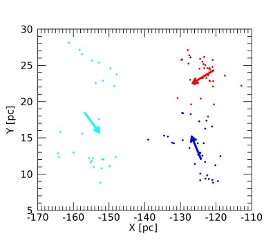
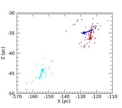
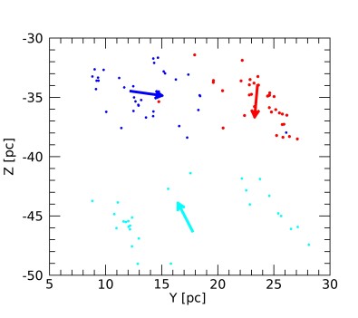
Figure 8: Spatial distribution (as in Fig. 7) of Taurus A (red), B (blue), and E (cyan), represented by the small dots, with RV measurements. The arrows represent the differential space velocities (U,V,W) with respect to the mean motion between all the sources of the three populations. Each differential value has been magnified by 100.

We use the available radial velocities collected from the literature by Galli et al. (2019). All three populations have radial velocity measurements for more than 20 stars; the corresponding histograms are shown in Fig. 10. Although the accuracy of these measurements does not allow a proper investigation of possible subclusterings, we can in any case see that, while Taurus A and B share a similar peak of the distribution, the peak of Taurus E is shifted by $\sim$1 km/s.
We computed the galactic space velocity (U, V, W) in the same reference system as the (X,Y,Z) positions computed in Sect. 4.2. These velocities have also been corrected for the solar motion to the local standard of rest. We considered the mean 3D velocities between Taurus A, B, and E as a reference to compute the mean differential velocities of each population. The results are shown in Fig. 8 with the three projections of the 3D average motions on the planes (X,Y), (X,Z), and (Y,Z). As discussed above, Taurus A and B are overlayed in the (X,Z) projection, and the relative motions can be misleading. In the (X,Y) projection, Taurus A and B are converging to a common point, while in the (Y,Z) projection, Taurus B is moving in the direction of Taurus A. This might be evidence that the two populations are merging. In two out of three projections, Taurus E appears to be approaching Taurus A and B.
Additional high-precision radial velocities of each member, in combination with astrometric data, are required to understand the dynamics of the entire region.

5 Summary and Conclusions

We carried out a statistical analysis (taking into account errors and covariances between the parameters) of the Taurus members with a reliable Gaia DR2 counterpart in order to look for multiple populations in the Taurus complex. Our results allow us to infer detailed information on the relation between the stellar population and the molecular cloud structures in the Herschel maps.
We find six stellar populations. Three of them are located over Taurus Main: Taurus A and B at a similar distance of $\sim$ 130 pc, and Taurus E at $\sim$ 160 pc. We find that these stellar populations lie at a similar distance to the molecular cloud when this is structured as a cloud, suggesting that they are associated. This is not the case when the molecular cloud is filamentary. Taurus C and F are mostly concentrated on the L1517 and L1551 clouds. The sixth population, Taurus D, is widely spread spatially and kinematically, suggesting it could either be a sparse young population, or be composed of multiple substructures.
The analysis of the differential average velocity suggests that Taurus A and B might be merging, while Taurus E is proceeding towards Taurus A and B. However, a definitive conclusion on their kinematics will only be possible when accurate radial velocities become available for all the members.

This study supports the view that star formation occurred in clumpy and filamentary structures that are evolving independently, and that Taurus is not the result of the expansion of a single star-formation episode.

Appendix A Additional material

Here, Table 3 provides a reduced version of the complete table of membership probabilities; the complete table is available online. Figure 9 shows the 3D spatial distribution of the six populations, which can be rotated in the electronic version of the paper. The histograms in Fig. 10 show the distribution of the radial velocity compiled from the literature for Taurus A, B, and E.

Table 3: Reduced first ten lines of the table available in the online version. RA and DEC positions and the astrometric data are from Gaia, the spectral types and the colors in the “pop” column are from Luhman (2018), the “clust” and “mem” columns are the cluster number and membership from Galli et al. (2019).

Name	Gaia DR2 ID	RA	DEC	PLX	E_PLX	PMRA	E_PMRA	PMDE	E_PMDE
AB Aur	156917493449670656	73.9410446	30.5510888	6.13996	0.05709	3.92615	0.09673	-24.11163	0.06753	…
CX Tau	162758236656524416	63.6994652	26.8029627	7.81673	0.03963	9.02460	0.10009	-22.45099	0.06506	…
DL Tau	148010281032823552	68.4128640	25.3438374	6.27593	0.04767	9.32913	0.08686	-18.29044	0.06509	…
FM Tau	163184366130809472	63.5566418	28.2135524	7.57948	0.04656	8.58744	0.10322	-24.41631	0.06664	…
FT Tau	149623711269425408	65.9133224	24.9371978	7.82449	0.05194	6.91801	0.11914	-21.69847	0.07524	…
GM Tau	148449845165337600	69.5889388	26.1537301	7.22990	0.14906	5.46909	0.26974	-22.97363	0.21549	…
GO Tau	148106316500918272	70.7628400	25.3384431	6.91711	0.04803	4.72669	0.10092	-20.20513	0.04601	…
HD 28354	152189662169148288	67.3326699	27.4041113	7.28903	0.10899	7.26521	0.17405	-25.14882	0.13331	…
LkCa 15	144936836795636864	69.8241791	22.3508662	6.29465	0.04814	10.47118	0.12711	-17.38300	0.05969	…
LkCa 19	156900622818205312	73.9040623	30.2985351	6.26297	0.07864	4.30736	0.15384	-24.13216	0.07560	…

	ruwe	$p_{A}$	$p_{B}$	$p_{C}$	$p_{D}$	$p_{E}$	$p_{F}$	RV	SpType	pop	clust	mem
…	1.02	0.00	0.00	0.98	0.02	0.00	0.00	8.90	A0	cyan	1	1
…	1.09	0.41	0.59	0.00	0.00	0.00	0.00	16.63	M2.5	red	7	0
…	1.16	0.00	0.00	0.00	0.01	0.99	0.00	13.94	K5.5	blue	13	1
…	1.27	1.00	0.00	0.00	0.00	0.00	0.00	…	M4.5	red	7	1
…	1.09	0.00	0.99	0.00	0.00	0.00	0.00	17.24	M3	red	9	1
…	1.23	0.01	0.91	0.00	0.08	0.00	0.00	16.46	M5	red	14	0
…	1.09	0.00	0.24	0.00	0.76	0.00	0.00	15.42	M2.3	red	15	1
…	1.10	0.99	0.00	0.00	0.01	0.00	0.00	…	B9	red	7	0
…	1.18	0.00	0.00	0.00	0.00	1.00	0.00	17.65	K5.5	blue	18	0
…	1.02	0.00	0.00	1.00	0.00	0.00	0.00	13.58	K2	cyan	1	1

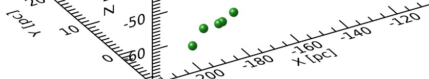
Figure 9: Three-dimensional spatial distribution of the multiple populations centered around the galactic center. The color code is as in Fig. 4. An animation with different orientation of this plot is available in the online version of the paper.

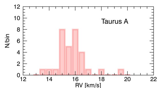
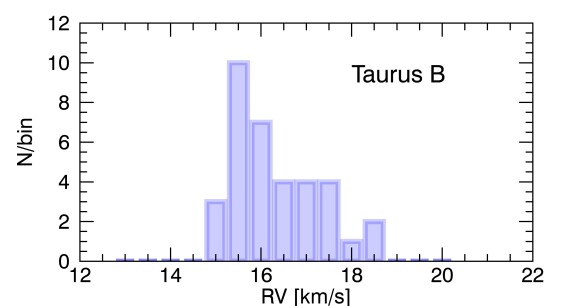
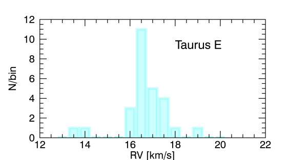
Figure 10: Distribution of radial velocities from Galli et al. (2019) for the most probable members of the Taurus A (red), Taurus B (blue), and the Taurus E (cyan) populations.