ICAS 049/20

MPP-2020-38

Mixed QCD$\otimes$QED corrections to exclusive Drell Yan
production using the $q_{T}$-subtraction method
Leandro Cieri^(a), Daniel de Florian^(b), Manuel Der^(b) and Javier Mazzitelli^(c)
(a) INFN, Sezione di Firenze, I-50019 Sesto Fiorentino, Florence, Italy

^(b)International Center for Advanced Studies (ICAS), ICIFI and ECyT-UNSAM,

25 de Mayo y Francia, (1650) Buenos Aires, Argentina

^(c)Max-Planck-Institut für Physik, Föhringer Ring 6, 80805 München, Germany

Abstract

In this work we extend the $q_{T}$-subtraction formalism, originally developed for QCD corrections, to the case of mixed QCD$\otimes$QED corrections, and apply it to the fully exclusive calculation of the ${\cal{O}}(\alpha_{s}\alpha)$ contribution to the production of an off-shell $Z$ boson in hadronic collisions. We present explicit results for the subtraction term and the hard factor, therefore providing all the ingredients needed for the application of the formalism up to ${\cal{O}}(\alpha_{s}\alpha)$. To study the phenomenological impact we consider the decay of the off-shell $Z$ boson into a pair of neutrinos, and present kinematical distributions for the final-state leptons at LHC energies.

1 Introduction

The Large Hadron Collider (LHC) at CERN is reaching, for many observables, an impressive accuracy. The precision of the LHC measurements will be further enhanced in the next runs and even more in the High-Luminosity upgrade of the LHC (HL-LHC). Theory must be ready for this appointment, producing equally accurate instruments in order to interpret the high-precision data. In this framework, QCD corrections play a crucial role. However, higher order perturbative QCD corrections for many observables and benchmark processes are of the same order of QED/EW or mixed QCD-EW theoretical predictions. Next-to-next-to-leading order (NNLO) QCD theoretical predictions (the standard of theoretical precision) for observables measured at the LHC are quite accurate but, in many cases, they are not sufficient to match the current accuracy at the experimental level and the new precision that will be reached in the following years. This scenario motivates a new theoretical effort to go beyond NNLO QCD corrections by including the first QED/EW corrections, mixed QCD-EW contributions and even the next QCD perturbative order: the next-to-next-to-next-to-leading order (${\rm N^{3}LO}$).

The Drell-Yan (DY) mechanism [1] (a benchmark process at modern colliders) constitutes a clear example of the statements of a precision observable. This process offers the possibility of studying fundamental electroweak (EW) parameters in a clean and accurate way. It also provides strong tests for QCD predictions and stringent information to determine parton distribution functions (PDFs) with high accuracy. The experimental precision for the DY mechanism at the LHC is at the percent level for the total cross section, and the differential distributions are also measured at an impressively high accuracy. The perturbative QCD corrections have been computed at next-to-leading order (NLO) in ref. [2], at NNLO for the inclusive cross section in refs. [3, 4, 5] and considering differential distributions in refs. [6, 7, 8, 9, 10, 11]. In addition, threshold expansions have been also presented at ${\rm N^{3}LL}$ accuracy in association with soft-virtual cross sections at ${\rm N^{3}LO}$ in refs. [12, 13]. Very recently, the ${\rm N^{3}LO}$ QCD corrections have been obtained for the inclusive cross section for the production of a lepton pair via virtual photon exchange [14].

However, computing several terms in the $\alpha_{s}$ expansion is not enough to reach the ultimate accuracy goal, since the EW coupling $\alpha$ satisfies $\alpha\sim\alpha_{s}^{2}$, and therefore NLO EW corrections, i.e. ${\cal O}(\alpha)$, are expected to be of the same order as the NNLO QCD contributions.

The calculation of NLO EW corrections for the DY process has been addressed in refs. [15, 16, 17] and [18, 19] for charged currents (CC) and neutral currents (NC), respectively. In order to improve our understanding of these EW effects, the calculation of their first order QCD corrections, i.e. the ${\cal O}(\alpha_{s}\alpha)$, becomes necessary. These corrections represent the first term in the fixed order expansion that takes into account mixed effects from the strong and electroweak interactions.

Different approaches have been followed in the literature in order to approximately combine the QCD and EW corrections [20, 21, 22, 23, 24], by either assuming the full factorisation or the additive combination of the strong and electroweak contributions. Partial exclusive results have been presented for the resonance region, by relying on the pole approximation [25, 26, 27].

A perturbative calculation of the Drell-Yan mechanism can be characterised by the following subsets: on one hand, purely factorisable terms that arise due to initial state (production, from the initial state partons) and final state (decay, from the final state leptons) emission and, on the other hand, non-factorisable terms originated by soft photon exchange between the production and the decay. The non-factorisable $\mathcal{O}(\alpha_{s}\alpha)$ terms have been shown [26, 25, 27] to have a negligible impact on the cross section, allowing to treat effectively Drell-Yan in the (resonant) limit of the decoupling between the production and decay processes, at least for the achieved experimental accuracy. Several steps towards the computation of the (inclusive) initial state QCD$\times$EW corrections have been recently carried out in an analytical way [28, 29, 30]. The appearance of massive gauge bosons results in extra complications, so it seems natural to start by looking at the case of QED contributions instead.

The first computation of the mixed QCD$\otimes$QED $\mathcal{O}(\alpha_{s}\alpha)$ corrections to the inclusive on-shell production of a $Z$ boson in hadronic collisions was achieved in ref. [31], by profiting from the available NNLO pure QCD corrections via the so-called abelianisation techniques [32, 33]. Those contributions were shown to be of the order of the NNLO QCD corrections for LHC energies, which makes them relevant to reach an accurate theoretical description. Moreover, it would be highly desirable to evaluate their effect at a fully exclusive level.

A crucial ingredient in the calculation of fully differential distributions are the so-called subtraction methods. For the case of pure QCD corrections to the hadroproduction of colourless final states, the $q_{T}$-subtraction method [34, 35] has been extensively used in order to obtain NNLO-accurate predictions. In this work, we extend the $q_{T}$-subtraction formalism in order to apply it to the calculation of ${\cal O}(\alpha_{s}\alpha)$ mixed corrections at a fully exclusive level. Our results are of value for transverse-momentum resummation at the corresponding logarithmic accuracy.

In particular, we will focus on the mixed QCD$\otimes$QED corrections to the production of an off-shell $Z$ boson decaying into a neutrino-antineutrino system. We consider the simplest case of uncharged particles in the decay of the off-shell $Z$ boson as a way to directly address the relevance on initial state corrections to a number of exclusive observables. Note that a recent work [36] also considers the production of a $Z$ boson, though in this case on-shell, in a fully exclusive way, based on the abelianised version of the nested soft-collinear subtraction formalism [37].

This paper is organised as follows: In Section 2 we present the relevant formulae for the extension of the $q_{T}$-subtraction method to the QCD$\otimes$QED case. In Section 3 we present our numerical results and study the phenomenology of the corrections for different kinematical variables. Finally, in Section 4 we present our conclusions.

2 Mixed order corrections with $q_{T}$-subtraction formalism

We consider the inclusive hard-scattering reaction

$$h_{1}(p_{1})+h_{2}(p_{2})\rightarrow F(M,q_{T})+X\,,$$ (1)

where the collision of the two hadrons $h_{1}$ and $h_{2}$ with momenta $p_{1}$ and $p_{2}$ produces the triggered generic final state $F$, without colour and electric charge, such as one or more neutral vector bosons ($\gamma^{*},Z,ZZ,\gamma\gamma$, $\ldots$), Higgs particles, and so forth. The observed final state $F$ is accompanied by the final-state radiation $X$, which in this case, consists of either quarks, antiquarks, gluons or photons. The system $F$ is composed by $n$ final-state particles with momenta $q_{1},q_{2},\dots,q_{n}$, and has total invariant mass $M^{2}=(q_{1}+q_{2}+\dots+q_{n})^{2}$, transverse momentum $q_{T}$ and rapidity $y$. We use $\sqrt{s}$ to denote the centre-of-mass energy of the colliding hadrons, which are treated in the massless approximation ($s=(p_{1}+p_{2})^{2}=2p_{1}\cdot p_{2}$).

We start by considering the QCD$\otimes$QED perturbative expansion of the (differential) cross section for the production of the final state $F$, by expanding in powers of the strong ($\alpha_{s}$) and electromagnetic ($\alpha$) couplings,

$$d\sigma^{F}=\sum_{i,j}\left(\frac{\alpha_{s}}{\pi}\right)^{i}\left(\frac{\alpha}{\pi}\right)^{j}d\sigma^{(i,j)}_{F},$$ (2)

where $d\sigma^{(i,0)}_{F}$ stands for the pure QCD corrections, and $d\sigma^{(0,j)}_{F}$ for the pure QED ones. The mixed corrections are represented by $d\sigma^{(i,j)}_{F}$ with both $i,j\neq 0$, being the first mixed contribution $d\sigma^{(1,1)}_{F}$.

Following a similar structure to the one valid in the pure QCD case [34, 35], the basic formula for the ${q_{T}}$-subtraction method in the case of mixed QCD$\otimes$QED corrections can be expressed in the following way,

$$d\sigma_{F}^{(1,1)}={\cal{H}}_{F}^{(1,1)}\otimes d\sigma_{F}^{(0,0)}+\left[d\sigma^{(1,1)}_{F+{\rm jet}}-d\sigma^{(1,1)}_{F\,CT}\right]\,,$$ (3)

where $d\sigma^{(1,1)}_{F+{\rm jet}}$ corresponds to the $F+\rm{jet}$ production cross section at ${\cal O}(\alpha_{s}\alpha)$. It is important to note that in this context ‘$\rm{jet}$’ stands for either quarks, antiquarks, gluons or photons in the final state and all of them need to be considered in the initial state as well. The term inside the square bracket in eq. (3) is finite in the limit of vanishing transverse momentum of the $F$ state, but the individual terms $d\sigma^{(1,1)}_{F+{\rm jet}}$ and $d\sigma^{(1,1)}_{F\,CT}$ are separately divergent. In order to evaluate $d\sigma^{(1,1)}_{F+{\rm jet}}$, we can make use of any NLO subtraction method (adapted, though, to the case of mixed QCD$\otimes$QED corrections).

The subtraction counter-term $d\sigma^{(1,1)}_{F\,CT}$ encodes the singular behaviour of the real scattering amplitudes in the small-$q_{T}$ region. The coefficient function ${\cal{H}}_{F}^{(1,1)}$ restores the correct normalisation to the total cross section and it has Born kinematics (e.g. it is proportional to $\delta(q_{T})$). Both coefficient functions can be obtained, through the abelianisation procedures [33, 32], from eqs. (63-70) in ref. [38]. We have checked (as a self-consistency check) that the same coefficient functions can be obtained from first principles, i.e redefining eq. (6) in ref. [35] to take into account QED emissions and expanding it to a given fixed order.

We present in the following the explicit expression of all the required terms needed for the subtraction at ${\cal O}(\alpha_{s}\alpha)$. These are constructed by convoluting the parton distributions with the corresponding partonic terms, which up to ${\cal O}(\alpha_{s}\alpha)$ are given by

$$d\sigma_{ab\,CT}^{F} =\left(\frac{\alpha_{s}}{\pi}\right)\,d\sigma^{F\,(1,0)}_{ab\,CT}+\left(\frac{\alpha}{\pi}\right)\,d\sigma^{F\,(0,1)}_{ab\,CT}+\left(\frac{\alpha_{s}}{\pi}\right)\left(\frac{\alpha}{\pi}\right)\,d\sigma^{F\,(1,1)}_{ab\,CT}$$

$$=\sum_{c}d\sigma_{c\overline{c},F}^{(0,0)}\Bigg{\{}\left(\frac{\alpha_{s}}{\pi}\right)\widetilde{\Sigma}_{c\overline{c}\leftarrow ab}^{F(1,0)}\left(z,q_{T}/Q\right)+\left(\frac{\alpha}{\pi}\right)\widetilde{\Sigma}_{c\overline{c}\leftarrow ab}^{F(0,1)}\left(z,q_{T}/Q\right)$$ (4)

$$+\left(\frac{\alpha_{s}}{\pi}\right)\left(\frac{\alpha}{\pi}\right)\widetilde{\Sigma}_{c\overline{c}\leftarrow ab}^{F(1,1)}\left(z,q_{T}/Q\right)\Bigg{\}}$$

and

$$\mathcal{H}_{ab}^{F}\otimes d\sigma_{LO}^{F} =\left[1+\left(\frac{\alpha_{s}}{\pi}\right)\,\mathcal{H}_{ab}^{F(1,0)}+\left(\frac{\alpha}{\pi}\right)\,\mathcal{H}_{ab}^{F(0,1)}+\left(\frac{\alpha_{s}}{\pi}\right)\left(\frac{\alpha}{\pi}\right)\,\mathcal{H}_{ab}^{F(1,1)}\right]\otimes d\sigma_{LO}^{F}$$

$$=\sum_{c}d\sigma_{c\overline{c},F}^{(0,0)}\Bigg{\{}\delta_{ca}\delta_{\overline{c}b}\delta(1-z)+\left(\frac{\alpha_{s}}{\pi}\right)\mathcal{H}_{c\overline{c}\leftarrow ab}^{F(1,0)}\left(z\right)$$ (5)

$$+\left(\frac{\alpha}{\pi}\right)\mathcal{H}_{c\overline{c}\leftarrow ab}^{F(0,1)}\left(z\right)+\left(\frac{\alpha_{s}}{\pi}\right)\left(\frac{\alpha}{\pi}\right)\mathcal{H}_{c\overline{c}\leftarrow ab}^{F(1,1)}\left(z\right)\Bigg{\}}\,.$$

In order to simplify the notation, we indicate by $z$ the dependence on both partonic momentum fractions $z_{1}$ and $z_{2}$. The explicit dependence on either $z_{1}$ and $z_{2}$ can be easily understood in terms on the dependence on the partonic label $a$ and $b$, respectively. Also, it is implicit the dependence on the renormalisation ($\mu_{R}$), factorisation ($\mu_{F}$) and resummation ($Q$) scales.

Note that, for the sake of generality, in the results contained in this section we keep the full dependence on the resummation scale [38]. This dependence is needed in the context of transverse-momentum resummation. The fixed-order cross-section is independent of this scale, and it is convenient to set $Q=M$ to simplify the corresponding expressions.

The contributions to the counter-term $\widetilde{\Sigma}_{c\overline{c}\leftarrow ab}^{F(i,j)}$ can be organized in the following way

$$\widetilde{\Sigma}_{c\overline{c}\leftarrow ab}^{F(1,0)}(z,q_{T}/Q)=\Sigma_{c\overline{c}\leftarrow ab}^{F(1,0)[1;2]}(z)\widetilde{I}_{2}\left(q_{T}/Q\right)+\Sigma_{c\overline{c}\leftarrow ab}^{F(1,0)[1;1]}(z)\widetilde{I}_{1}\left(q_{T}/Q\right)\,,$$ (6)

$$\widetilde{\Sigma}_{c\overline{c}\leftarrow ab}^{F(0,1)}(z,q_{T}/Q)=\Sigma_{c\overline{c}\leftarrow ab}^{F(0,1)[1;2]}(z)\widetilde{I}_{2}\left(q_{T}/Q\right)+\Sigma_{c\overline{c}\leftarrow ab}^{F(0,1)[1;1]}(z)\widetilde{I}_{1}\left(q_{T}/Q\right)\,,$$ (7)

$$\widetilde{\Sigma}_{c\overline{c}\leftarrow ab}^{F(1,1)}(z,q_{T}/Q) =\Sigma_{c\overline{c}\leftarrow ab}^{F(1,1)[2;4]}(z)\widetilde{I}_{4}\left(q_{T}/Q\right)+\Sigma_{c\overline{c}\leftarrow ab}^{F(1,1)[2;3]}(z)\widetilde{I}_{3}\left(q_{T}/Q\right)$$

$$\,+\Sigma_{c\overline{c}\leftarrow ab}^{F(1,1)[2;2]}(z)\widetilde{I}_{2}\left(q_{T}/Q\right)+\Sigma_{c\overline{c}\leftarrow ab}^{F(1,1)[2;1]}(z)\widetilde{I}_{1}\left(q_{T}/Q\right)\,,$$ (8)

according to their power of logarithmic enhancement. The dependence on the transverse momentum is given by the known integrals [38]

$$\widetilde{I}_{n}\left(q_{T}/Q\right)=Q^{2}\int_{0}^{\infty}db\frac{b}{2}J_{0}\left(bq_{T}\right)\ln^{n}\left(\frac{Q^{2}b^{2}}{b_{0}^{2}}+1\right)\,,$$ (9)

where $b$ is the impact parameter, $J_{0}(x)$ is the 0th-order Bessel function and $b_{0}=2e^{-\gamma_{E}}$, with $\gamma_{E}$ representing the Euler number. Notice that we are using the “$+1$” prescription (see the argument of the logarithm inside eq. (9)), and therefore, the counter-terms vanish in the large-$q_{T}$ limit. More details about eq. (9) can be found in the Appendix A of ref. [38].

The corresponding coefficients for the expansion of $\widetilde{\Sigma}_{c\overline{c}\leftarrow ab}^{F(i,j)}$ and $\mathcal{H}_{c\overline{c}\leftarrow ab}^{F(i,j)}$ are more easily presented by considering their $N$-moments (Mellin) with respect to the variable $z$. At NLO in QCD and QED they are given by

$$\Sigma_{c\overline{c}\leftarrow ab,N}^{F(1,0)[1;2]}=-\frac{1}{2}A_{c}^{(1,0)}\delta_{ca}\delta_{\overline{c}b}\,,$$ (10)

$$\Sigma_{c\overline{c}\leftarrow ab,N}^{F(1,0)[1;1]}=-\left[\delta_{ca}\delta_{\overline{c}b}\left(B_{c}^{(1,0)}+A_{c}^{(1,0)}\ell_{Q}\right)+\delta_{ca}\gamma_{\overline{c}b,N}^{(1,0)}+\delta_{\overline{c}b}\gamma_{ca,N}^{(1,0)}\right]\,,$$ (11)

$$\Sigma_{c\overline{c}\leftarrow ab,N}^{F(0,1)[1;2]}=-\frac{1}{2}A_{c}^{(0,1)}\delta_{ca}\delta_{\overline{c}b}\,,$$ (12)

$$\Sigma_{c\overline{c}\leftarrow ab,N}^{F(0,1)[1;1]}=-\left[\delta_{ca}\delta_{\overline{c}b}\left(B_{c}^{(0,1)}+A_{c}^{(0,1)}\ell_{Q}\right)+\delta_{ca}\gamma_{\overline{c}b,N}^{(0,1)}+\delta_{\overline{c}b}\gamma_{ca,N}^{(0,1)}\right]\,,$$ (13)

$$\mathcal{H}_{c\overline{c}\leftarrow ab,N}^{F(1,0)} =\delta_{ca}\delta_{\overline{c}b}\left[H_{c}^{F(1,0)}-\left(B_{c}^{(1,0)}+\frac{1}{2}A_{c}^{(1,0)}\ell_{Q}\right)\ell_{Q}\right]$$ (14)

$$+\delta_{ca}C_{\overline{c}b,N}^{(1,0)}+\delta_{\overline{c}b}C_{ca,N}^{(1,0)}+\left(\delta_{ca}\gamma_{\overline{c}b,N}^{(1,0)}+\delta_{\overline{c}b}\gamma_{ca,N}^{(1,0)}\right)\left(\ell_{F}-\ell_{Q}\right)\,,$$

$$\mathcal{H}_{c\overline{c}\leftarrow ab,N}^{F(0,1)} =\delta_{ca}\delta_{\overline{c}b}\left[H_{c}^{F(0,1)}-\left(B_{c}^{(0,1)}+\frac{1}{2}A_{c}^{(0,1)}\ell_{Q}\right)\ell_{Q}\right]$$ (15)

$$+\delta_{ca}C_{\overline{c}b,N}^{(0,1)}+\delta_{\overline{c}b}C_{ca,N}^{(0,1)}+\left(\delta_{ca}\gamma_{\overline{c}b,N}^{(0,1)}+\delta_{\overline{c}b}\gamma_{ca,N}^{(0,1)}\right)\left(\ell_{F}-\ell_{Q}\right)\,,$$

while for the mixed QCD$\otimes$QED corrections at ${\cal O}(\alpha_{s}\alpha)$ they are given by

$$\Sigma_{c\overline{c}\leftarrow ab,N}^{F(1,1)[2;4]}=\frac{1}{4}A_{c}^{(1,0)}A_{c}^{(0,1)}\delta_{ca}\delta_{\overline{c}b}\,,$$ (16)

$$\Sigma_{c\overline{c}\leftarrow ab,N}^{F(1,1)[2;3]}=-A_{c}^{(0,1)}\frac{1}{2}\Sigma_{c\overline{c}-ab,N}^{F(1,0)[1;1]}-A_{c}^{(1,0)}\frac{1}{2}\Sigma_{c\overline{c}-ab,N}^{F(0,1)[1;1]}\,,$$ (17)

$$\Sigma_{c\overline{c}\leftarrow ab,N}^{F(1,1)[2;2]}= -\frac{1}{2}A_{c}^{(1,0)}\mathcal{H}_{c\overline{c}\leftarrow ab,N}^{F(0,1)}-\frac{1}{2}\sum_{a_{1},b_{1}}\Sigma_{c\overline{c}\leftarrow a_{1}b_{1},N}^{F(1,0)[1;1]}\left[\delta_{a_{1}a}\gamma_{b_{1}b,N}^{(0,1)}+\delta_{b_{1}b}\gamma_{a_{1}a,N}^{(0,1)}\right]$$

$$-\frac{1}{2}A_{c}^{(0,1)}\mathcal{H}_{c\overline{c}\leftarrow ab,N}^{F(1,0)}-\frac{1}{2}\sum_{a_{1},b_{1}}\Sigma_{c\overline{c}\leftarrow a_{1}b_{1},N}^{F(0,1)[1;1]}\left[\delta_{a_{1}a}\gamma_{b_{1}b,N}^{(1,0)}+\delta_{b_{1}b}\gamma_{a_{1}a,N}^{(1,0)}\right]$$ (18)

$$-\frac{1}{2}\left[A_{c}^{(1,1)}\delta_{ca}\delta_{\overline{c}b}+\left(B_{c}^{(1,0)}+A_{c}^{(1,0)}\ell_{Q}\right)\Sigma_{c\overline{c}\leftarrow ab,N}^{F(0,1)[1;1]}+\left(B_{c}^{(0,1)}+A_{c}^{(0,1)}\ell_{Q}\right)\Sigma_{c\overline{c}\leftarrow ab,N}^{F(1,0)[1;1]}\right]\,,$$

$$\Sigma_{c\overline{c}\leftarrow ab,N}^{F(1,1)[2;1]}= -\sum_{a_{1},b_{1}}\mathcal{H}_{c\overline{c}\leftarrow a_{1}b_{1},N}^{F(1,0)}\left[\delta_{a_{1}a}\delta_{b_{1}b}\left(B_{c}^{(0,1)}+A_{c}^{(0,1)}\ell_{Q}\right)+\delta_{a_{1}a}\gamma_{b_{1}b,N}^{(0,1)}+\delta_{b_{1}b}\gamma_{a_{1}a,N}^{(0,1)}\right]$$ (19)

$$-\sum_{a_{1},b_{1}}\mathcal{H}_{c\overline{c}\leftarrow a_{1}b_{1},N}^{F(0,1)}\left[\delta_{a_{1}a}\delta_{b_{1}b}\left(B_{c}^{(1,0)}+A_{c}^{(1,0)}\ell_{Q}\right)+\delta_{a_{1}a}\gamma_{b_{1}b,N}^{(1,0)}+\delta_{b_{1}b}\gamma_{a_{1}a,N}^{(1,0)}\right]$$

$$-\left[\delta_{ca}\delta_{\overline{c}b}\left(B_{c}^{(1,1)}+A_{c}^{(1,1)}\ell_{Q}\right)+\delta_{ca}\gamma_{\overline{c}b,N}^{(1,1)}+\delta_{\overline{c}b}\gamma_{ca,N}^{(1,1)}\right]\,,$$

$$\mathcal{H}_{c\overline{c}\leftarrow ab,N}^{F(1,1)} =\delta_{ca}\delta_{\overline{c}b}H_{c}^{F(1,1)}+\delta_{ca}C_{\overline{c}b,N}^{(1,1)}+\delta_{\overline{c}b}C_{ca,N}^{(1,1)}+C_{ca,N}^{(1,0)}C_{\overline{c}b,N}^{(0,1)}+C_{ca,N}^{(0,1)}C_{\overline{c}b,N}^{(1,0)}$$

$$+H_{c}^{F(1,0)}\left(\delta_{ca}C_{\overline{c}b,N}^{(0,1)}+\delta_{\overline{c}b}C_{ca,N}^{(0,1)}\right)+H_{c}^{F(0,1)}\left(\delta_{ca}C_{\overline{c}b,N}^{(1,0)}+\delta_{\overline{c}b}C_{ca,N}^{(1,0)}\right)$$

$$+\frac{1}{2}A_{c}^{(1,1)}\delta_{ca}\delta_{\overline{c}b}\ell_{Q}^{2}+\left(\delta_{ca}\gamma_{\overline{c}b,N}^{(1,1)}+\delta_{\overline{c}b}\gamma_{ca,N}^{(1,1)}\right)\ell_{F}$$

$$-\left[\delta_{ca}\delta_{\overline{c}b}\left(B_{c}^{(1,1)}+A_{c}^{(1,1)}\ell_{Q}\right)+\delta_{ca}\gamma_{\overline{c}b,N}^{(1,1)}+\delta_{\overline{c}b}\gamma_{ca,N}^{(1,1)}\right]\ell_{Q}$$

$$+\frac{1}{2}\sum_{a_{1},b_{1}}\left[\mathcal{H}_{c\overline{c}\leftarrow a_{1}b_{1},N}^{F(1,0)}+\delta_{ca_{1}}\delta_{\overline{c}b_{1}}H_{c}^{F(1,0)}+\delta_{ca_{1}}C_{\overline{c}b_{1},N}^{(1,0)}+\delta_{\overline{c}b_{1}}C_{ca_{1},N}^{(1,0)}\right]$$ (20)

$$\;\;\;\;\;\times\left[\left(\delta_{a_{1}a}\gamma_{b_{1}b,N}^{(0,1)}+\delta_{b_{1}b}\gamma_{a_{1}a,N}^{(0,1)}\right)\left(\ell_{F}-\ell_{Q}\right)-\delta_{a_{1}a}\delta_{b_{1}b}\left(\left(B_{c}^{(0,1)}+\frac{1}{2}A_{c}^{(0,1)}\ell_{Q}\right)\ell_{Q}\right)\right]$$

$$+\frac{1}{2}\sum_{a_{1},b_{1}}\left[\mathcal{H}_{c\overline{c}\leftarrow a_{1}b_{1},N}^{F(0,1)}+\delta_{ca_{1}}\delta_{\overline{c}b_{1}}H_{c}^{F(0,1)}+\delta_{ca_{1}}C_{\overline{c}b_{1},N}^{(0,1)}+\delta_{\overline{c}b_{1}}C_{ca_{1},N}^{(0,1)}\right]$$

$$\;\;\;\;\;\times\left[\left(\delta_{a_{1}a}\gamma_{b_{1}b,N}^{(1,0)}+\delta_{b_{1}b}\gamma_{a_{1}a,N}^{(1,0)}\right)\left(\ell_{F}-\ell_{Q}\right)-\delta_{a_{1}a}\delta_{b_{1}b}\left(\left(B_{c}^{(1,0)}+\frac{1}{2}A_{c}^{(1,0)}\ell_{Q}\right)\ell_{Q}\right)\right]\,.$$

In the expressions above we have defined $\ell_{Q}=\ln M^{2}/Q^{2}$ and $\ell_{F}=\ln M^{2}/\mu_{F}^{2}$, while $\gamma_{ab,N}^{(i,j)}$ represent the corresponding (moments of the) splitting functions. The coefficients $A_{c}^{(i,j)}$ and $B_{c}^{(i,j)}$ arise from the expansion of the Sudakov form factor,

$$S_{c}(M,b)=\exp\left\{-\int_{b_{0}^{2}/b^{2}}^{M^{2}}\frac{dq^{2}}{q^{2}}\left[A_{c}\left(\alpha_{s},\alpha\right)\ln\frac{M^{2}}{q^{2}}+B_{c}\left(\alpha_{s},\alpha\right)\right]\right\}\,,$$ (21)

with

$$A_{c}\left(\alpha_{s},\alpha\right) =\left(\frac{\alpha_{s}}{\pi}\right)A_{c}^{(1,0)}+\left(\frac{\alpha}{\pi}\right)A_{c}^{(0,1)}+\left(\frac{\alpha_{s}}{\pi}\right)\left(\frac{\alpha}{\pi}\right)A_{c}^{(1,1)}+\dots\,,$$ (22)

$$B_{c}\left(\alpha_{s},\alpha\right) =\left(\frac{\alpha_{s}}{\pi}\right)B_{c}^{(1,0)}+\left(\frac{\alpha}{\pi}\right)B_{c}^{(0,1)}+\left(\frac{\alpha_{s}}{\pi}\right)\left(\frac{\alpha}{\pi}\right)B_{c}^{(1,1)}+\dots\,,$$

and their explicit expression for quark-initiated case is given by

$$A_{q}^{(1,0)}=C_{F}\,,\,\,\,\,\,\,\,\,\,A_{q}^{(0,1)}=e_{q}^{2}\,,$$

$$B_{q}^{(1,0)}=-\frac{3}{2}C_{F}\,,\,\,\,\,\,\,\,\,\,B_{q}^{(0,1)}=-\frac{3}{2}e_{q}^{2}\,,$$ (23)

$$A_{q}^{(1,1)}=0\,,\,\,\,\,\,\,\,\,\,B_{q}^{(1,1)}=\frac{C_{F}e_{q}^{2}}{8}(-3+24\zeta_{2}-48\zeta_{3})\,.$$

Notice that we consider the electromagnetic coupling $\alpha$ as constant, in the sense that it is not running with any of the scales related to the process. For that reason the QED beta-function does not appear in the coefficients of eqs. (10–2). Eqs. (10–15) were derived for first time in ref. [39], where the transverse-momentum resummation for $Z$ boson production combining QED and QCD was computed at NLO. It is worth noticing that for transverse-momentum resummation some novel mixed effects appear affecting the distribution already at leading logarithmic (LL) accuracy (see eqs. (7) and (11) of ref. [39]). Nevertheless, that contribution can only show up after performing the fixed order expansion up to $\mathcal{O}(\alpha_{s}\alpha)$ (see eq. (3) in ref. [39]) if the electromagnetic coupling $\alpha$ is considered to be running, which is not the case in our current study.

Finally we present the collinear functions, again for $c=q$, and the hard-virtual coefficients, the latter specifically for the DY case as they are a process-dependent quantity. The separation between $C$ and $H$ coefficients is scheme dependent. Those presented here are obtained in the so-called hard scheme [35]. Up to NLO in QCD and QED, the hard-virtual coefficients take the form

$$H_{q}^{DY(1,0)}=C_{F}\left(\frac{\pi^{2}}{2}-4\right)=\frac{C_{F}}{e_{q}^{2}}H_{q}^{DY(0,1)}\,,$$ (24)

and the collinear functions are given by

$$C_{qq}^{(1,0)}(z) =\frac{C_{F}}{2}(1-z)=\frac{C_{F}}{e_{q}^{2}}C_{qq}^{(0,1)}(z)\,,$$

$$C_{qg}^{(1,0)}(z) =\frac{1}{2}z(1-z)=C_{q\gamma}^{(0,1)}(z)\frac{T_{R}}{e_{q}^{2}N_{C}}\,,$$ (25)

$$C_{gq}^{(1,0)}(z) =\frac{C_{F}}{2}z=\frac{C_{F}}{e_{q}^{2}}C_{\gamma q}^{(0,1)}(z)\,.$$

The hard-virtual coefficient needed for the first order in the mixed QCD$\otimes$QED expansion takes the following form,

$$H_{q}^{DY(1,1)}=\frac{C_{F}e_{q}^{2}}{2}\left(-15\zeta_{3}+\frac{511}{16}-\frac{67\pi^{2}}{12}+\frac{17\pi^{4}}{45}\right)\,,$$ (26)

while the needed collinear functions are given by the following expressions:

$$C_{qq^{\prime}}^{(1,1)}(z) =\delta_{qq^{\prime}}\,e_{q}^{2}C_{F}\Bigg{\{}\frac{1+z^{2}}{1-z}\Bigg{(}\frac{\operatorname{Li}_{3}(1-z)}{2}+\frac{1}{2}\operatorname{Li}_{2}(z)\log(1-z)+\frac{3\operatorname{Li}_{2}(z)\log(z)}{2}$$

$$-\frac{5\operatorname{Li}_{3}(z)}{2}+\frac{3}{4}\log(z)\log^{2}(1-z)+\frac{1}{4}\log^{2}(z)\log(1-z)-\frac{1}{12}\pi^{2}\log(1-z)+\frac{5\zeta_{3}}{2}\Bigg{)}$$

$$+(1-z)\left(-\operatorname{Li}_{2}(z)-\frac{3}{2}\log(1-z)\log(z)+\frac{2\pi^{2}}{3}-\frac{29}{4}\right)+\frac{1}{24}(1+z)\log^{3}(z)$$ (27)

$$+\frac{1}{1-z}\left(\frac{1}{8}\left(-2z^{2}+2z+3\right)\log^{2}(z)+\frac{1}{4}\left(17z^{2}-13z+4\right)\log(z)\right)$$

$$-\frac{z}{4}\log(1-z)-\frac{1}{4}\left[(2\pi^{2}-18)(1-z)-(1+z)\log z\right]\Bigg{\}}\,,$$

$$C_{q\overline{q}^{\prime}}^{(1,1)}(z) =\delta_{qq^{\prime}}\,2C_{F}e_{q}^{2}\left\{\frac{1+z^{2}}{1+z}\left(\frac{3\operatorname{Li}_{3}(-z)}{2}+\operatorname{Li}_{3}(z)+\operatorname{Li}_{3}\left(\frac{1}{1+z}\right)-\frac{\operatorname{Li}_{2}(-z)\log(z)}{2}\right.\right.$$

$$-\frac{\operatorname{Li}_{2}(z)\log(z)}{2}-\frac{1}{24}\log^{3}(z)-\frac{1}{6}\log^{3}(1+z)+\frac{1}{4}\log(1+z)\log^{2}(z)$$

$$+\left.\frac{\pi^{2}}{12}\log(1+z)-\frac{3\zeta_{3}}{4}\right)+(1-z)\left(\frac{\operatorname{Li}_{2}(z)}{2}+\frac{1}{2}\log(1-z)\log(z)+\frac{15}{8}\right)$$ (28)

$$-\left.\frac{1}{2}(1+z)\left(\operatorname{Li}_{2}(-z)+\log(z)\log(1+z)\right)+\frac{\pi^{2}}{24}(z-3)+\frac{1}{8}(11z+3)\log(z)\right\}\,,$$

$$C_{qg}^{(1,1)}(z) =e_{q}^{2}\Bigg{\{}\left(2z^{2}-2z+1\right)\left(\zeta_{3}-\frac{\operatorname{Li}_{3}(1-z)}{8}-\frac{\operatorname{Li}_{3}(z)}{8}+\frac{1}{8}\operatorname{Li}_{2}(1-z)\log(1-z)\right.$$

$$\left.+\frac{\operatorname{Li}_{2}(z)\log(z)}{8}-\frac{1}{48}\log^{3}(1-z)+\frac{1}{16}\log(z)\log^{2}(1-z)+\frac{1}{16}\log^{2}(z)\log(1-z)\right)$$

$$-\frac{3z^{2}}{8}-\frac{1}{96}\left(4z^{2}-2z+1\right)\log^{3}(z)+\frac{1}{64}\left(-8z^{2}+12z+1\right)\log^{2}(z)$$ (29)

$$+\frac{1}{32}\left(-8z^{2}+23z+8\right)\log(z)+\frac{5}{24}\pi^{2}(1-z)z+\frac{11z}{32}+\frac{1}{8}(1-z)z\log^{2}(1-z)$$

$$-\frac{1}{4}(1-z)z\log(1-z)\log(z)-\frac{1}{16}(3-4z)z\log(1-z)-\frac{9}{32}$$

$$-\frac{1}{4}\left[z\log z+\frac{1}{2}\left(1-z^{2}\right)+\left(\pi^{2}-8\right)z(1-z)\right]\Bigg{\}}\,,$$

$$C_{q{\gamma}}^{(1,1)}(z)={2C_{F}C_{A}}C_{q{g}}^{(1,1)}(z)\,.$$ (30)

The results above provide all the ingredients needed for the application of the $q_{T}$-subtraction formalism to the calculation of mixed QCD$\otimes$QED corrections. The same coefficients are required by the transverse-momentum resummation formalism, considering in this case the full dependence on the resummation scale $Q$.

In the following section we present our phenomenological results for the case of $Z$ boson production.

3 Phenomenological results

In order to obtain quantitative results, our calculation is implemented in two independent parton-level Monte Carlo programs. One of them is based on MCFM [11] (including the NNLO QCD corrections), suitably modified to deal with mixed corrections and to apply the $q_{T}$-subtraction formalism. The other is a private implementation, which relies on the FKS subtraction method [40] to deal with the NLO-type divergencies (adapted to the mixed QCD$\otimes$QED case), and on analytic results for the relevant scattering amplitudes obtained from ref. [41], plus an explicit calculation of the tree-level all-quarks channels using FeynCalc 9.2.0 [42].

For our phenomenological analysis we consider $n_{F}=5$ massless quark flavours. We work in the $G_{\mu}$ scheme for the EW couplings, using the input values $G_{\mu}=1.16639\times 10^{-5}\text{~{}GeV}^{-2}$, $M_{Z}=91.1876$ GeV and $M_{W}=80.385$ GeV. The width of the $Z$ boson is set to the value $\Gamma_{Z}=2.4952$ GeV. For the parton luminosities and strong coupling, we use the NNPDF3.1luxQED set with five flavours [43] through the LHAPDF interface [44], always at NNLO accuracy, regardless the order of the calculation. Both renormalisation and factorisation scales are set to the default value $\mu_{R}=\mu_{F}=m_{\ell_{1}\ell_{2}}$. For the cutoff parameter of the subtraction method, $q_{T,\text{cut}}$, we choose the central value $q_{T,\text{cut}}=0.2$ GeV. We checked that our results are compatible within uncertainties when varying this parameter around its central value by a factor of 2.

As a first check of our implementation, we computed the inclusive cross section for the production of an on-shell $Z$ boson, and compared to the predictions obtained from the analytic results presented in ref. [31]. The corresponding ${\cal O}(\alpha_{s}\alpha)$ contributions to the cross section, split into quark-quark, quark-gluon, quark-photon and gluon-photon initiated channels, are shown in table 1. As can be seen from the table, we can reach sub-percent precision for these inclusive predictions, and we find full agreement with the analytic results from ref. [31]. As an additional validation, we have computed the NNLO QCD differential distributions using the public code Matrix [45], finding full agreement with our results.

Channel	$qq^{\prime}$	$qg$	$q\gamma$	$g\gamma$
$q_{T}$-subtraction [pb]	$52.6(4)$	$-34.8(3)$	$-1.41(1)$	$0.569(2)$
Analytic (ref. [31]) [pb]	$52.3$	$-35.0$	$-1.41$	$0.571$

Table 1: The ${\cal O}(\alpha_{s}\alpha)$ contribution to the inclusive on-shell $Z$ production cross section for the different partonic channels. The results obtained using $q_{T}$-subtraction are compared to the inclusive predictions obtained in ref. [31]. Numerical uncertainties on the last digit are indicated in parenthesis for our predictions, while the uncertainties of the inclusive implementation are below the last digits shown. The category denoted by $qq^{\prime}$ includes all combinations of quarks and anti-quarks.

For all of the differential distributions presented here, we consider the following set of cuts,

$$p_{T,\ell_{1}}>25\,{\rm GeV}\,,\,\,\,\,p_{T,\ell_{2}}>20\,{\rm GeV}\,,\,\,\,\,|y|_{\ell_{1,2}}<2.5\,,\,\,\,\,m_{\ell_{1}\ell_{2}}>50\,{\rm GeV,}$$ (31)

where $\ell_{1}$ and $\ell_{2}$ represent the final-state leptons, ordered according to their transverse momentum. Since we consider only neutrinos in the final state, there is no need to recombine collinear leptons and photons.

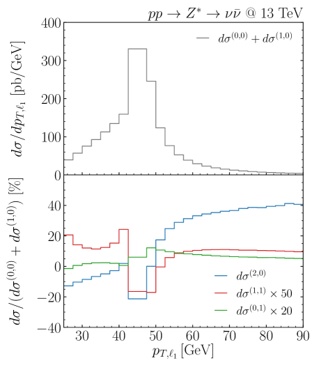
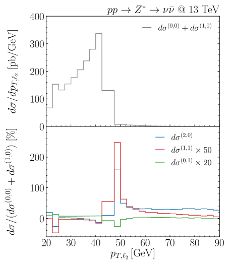
Figure 1: Transverse momentum distributions for the hardest (left) and softer (right) lepton. The upper panel shows the NLO QCD prediction, while the lower panel shows the NNLO QCD (blue), NLO QED (green) and mixed (red) corrections, normalized to the NLO result.

We start by presenting the transverse momentum distribution of the leptons in figure 1. The kinematical dependence of the mixed corrections is highly non trivial. This feature is also shared by the pure QCD and QED corrections, and it is expected due to the particular features that these two distributions present at fixed order in perturbation theory. At LO both leptons are back-to-back, and therefore the distributions are identical. The radiative corrections produce the change of shape that render the $p_{T,\ell_{1}}$ spectrum harder than the $p_{T,\ell_{2}}$ one, producing therefore sizeable distortions in the distribution. Furthermore, some regions of the phase space are almost not populated at LO, and therefore radiative corrections become more relevant. This is the case for the region of $p_{T,\ell_{2}}$ below the lower cut on $p_{T,\ell_{1}}$, which is directly not allowed for Born kinematics, or the region above $p_{T,\ell_{1,2}}\simeq M_{Z}/2$, which does not receive contributions from the $Z$ peak at LO.

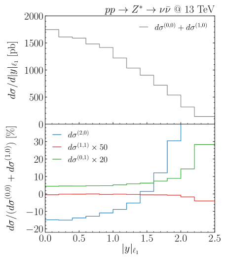
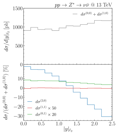
Figure 2: Rapidity distributions for the hardest (left) and softer (right) lepton. The upper panel shows the NLO QCD prediction, while the lower panel shows the NNLO QCD (blue), NLO QED (green) and mixed (red) corrections, normalized to the NLO result.

From figure 1 we can observe that for $p_{T,\ell_{1}}<M_{Z}/2$ the mixed corrections are positive, representing an increase of about $0.5\%$ with respect to the NLO prediction. The corrections then change sign, being of the order of $-0.5\%$ in the first bins after $p_{T,\ell_{1}}=M_{Z}/2$, which corresponds to the expected Sudakov shoulder near the kinematic boundaries mentioned in the previous paragraph [46]. The mixed corrections then result smaller at the tail of the distribution. With respect to the softer lepton, we can observe that the corrections become very large around and slightly above $p_{T,\ell_{2}}=M_{Z}/2$, a pattern shared by the NNLO QCD corrections. In this region, the effect of the mixed QCD$\otimes$QED contribution can reach the ${\cal O}(5\%)$ with respect to the NLO QCD result. In addition, we can also observe a small (negative) peak in the corrections around $p_{T,\ell_{2}}=25$ GeV, which is related to the presence of a cut in $p_{T,\ell_{1}}$, as mentioned before.

We continue by presenting the rapidity distributions of the leptons, again ordered according to their transverse momentum, in figure 2. In both cases, we can observe that the mixed corrections are extremely small, and show a very mild dependence on the corresponding kinematical variable. The reason for this particularly small value of the corrections is a very strong cancellation between the main partonic channels, that is the $q\bar{q}$ and $qg$ initiated processes, over the whole rapidity range under consideration, a pattern that can also be observed for instance at the level of the total cross section. We note that this effect is even stronger with the set of cuts in eq. (31), compared to the fully inclusive case, with cancellations of about $90\%$ between the different channels.

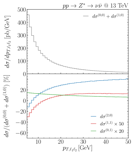
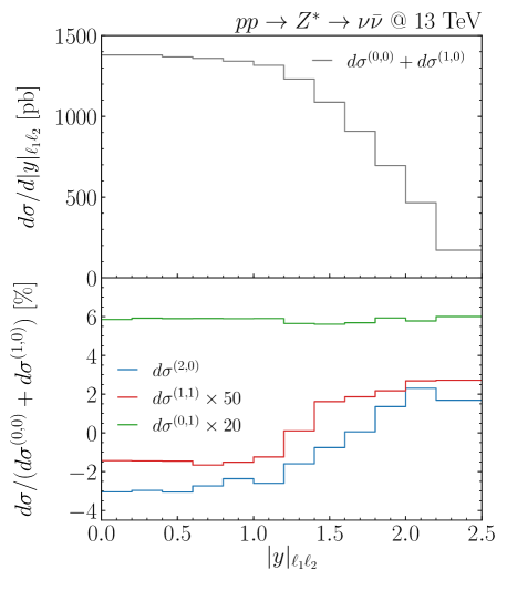
Figure 3: Lepton-pair transverse momentum (left) and rapidity (right) distributions. The upper panel shows the NLO QCD prediction, while the lower panel shows the NNLO QCD (blue), NLO QED (green) and mixed (red) corrections, normalized to the NLO result.

In figure 3 we present distributions for the lepton-pair system, specifically its transverse momentum and rapidity. The mixed corrections are negative below $p_{T,\ell_{1}\ell_{2}}\sim 15$ GeV, and diverge in the $p_{T,\ell_{1}\ell_{2}}\to 0$ limit. The sign of the mixed corrections in the low transverse momentum region is the same as the one of the NNLO QCD corrections, as one can infer from the sign of the logarithmic coefficient with highest power (see eq. (16) for the mixed corrections and eq. (66) of ref. [38] for NNLO QCD). Above $p_{T,\ell_{1}\ell_{2}}\sim 15$ GeV the mixed corrections become positive, increasing the NLO QCD result by about $0.3\%$. In the same region the NLO QED corrections are of the order of $0.5\%$. As it is well known, at low-$q_{T}$, the large logarithmic corrections to the cross section have to be treated with transverse momentum resummation in order to recover the reliability of the prediction. This is true not only for the transverse momentum distribution but for any observable which presents a kinematical region directly related to $q_{T}=0$.

The mixed corrections for the lepton-pair rapidity present a kinematic dependence that is similar to the one of the NNLO QCD contribution. They are negative for small $|y|_{\ell_{1}\ell_{2}}$, and become positive for larger values of rapidity. The overall size of the mixed corrections is of course much smaller though, being of the order of 50 times smaller than the NNLO QCD corrections.

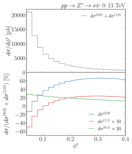
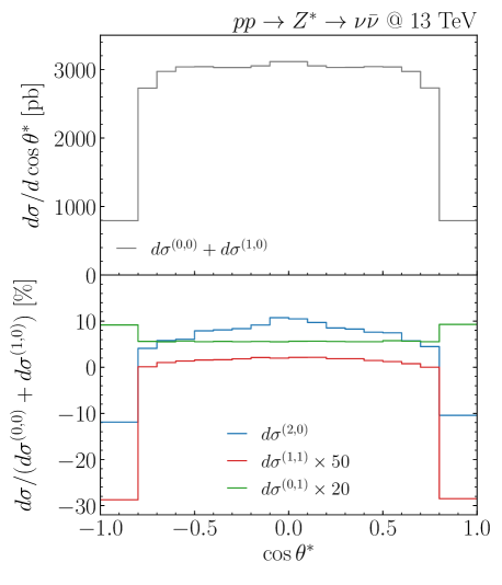
Figure 4: The $\phi^{*}$ distribution. The upper panel shows the NLO QCD prediction, while the lower panel shows the NNLO QCD (blue), NLO QED (green) and mixed (red) corrections, normalized to the NLO result.

Finally, we present in figure 4 the $\phi^{*}$ and $\cos\theta^{*}$ distributions, defined as [47]

$$\phi^{*}=\tan\left(\frac{\pi-\Delta\Phi}{2}\right)\sin\theta^{*}$$

$$\Delta\Phi=\phi_{\,\ell_{1}}-\phi_{\,\ell_{2}}$$ (32)

$$\cos\theta^{*}=\tanh\left(\frac{y_{\,\ell_{1}}-y_{\,\ell_{2}}}{2}\right)\,.$$

Since at LO the two leptons are back-to-back, the $\phi^{*}$ distribution is trivial at that order, and contributions with $\phi^{*}\neq 0$ only start at NLO. As in the case of the transverse momentum, the small-$\phi^{*}$ region is not well behaved at fixed order and it is necessary the use of transverse resummation in order to recover the reliability of the prediction in those kinematical regions. The pattern of corrections, not only for the mixed but also for the NNLO QCD and NLO QED contributions, is very similar to the one observed in the $p_{T,\ell_{1}\ell_{2}}$ distribution, in particular with the mixed corrections being negative at small $\phi^{*}$ and becoming positive for larger values, and about a factor of 2 smaller than the NLO QED corrections in the tail of the distribution.

In the case of $\cos\theta^{*}$, the distribution is rather flat in the central region, and presents a strong suppression for $\cos\theta^{*}=\pm 1$, which is only populated by events with very large and opposite rapidities of the corresponding leptons. This region is therefore particularly suppressed by the presence of the cuts on $y_{\,\ell_{1,2}}$, which directly forbid the region above $|\cos\theta^{*}|\sim 0.987$. From the lower panel of the figure we can observe that the perturbative corrections are rather flat in the region where the bulk of the cross section is located, and therefore they follow a pattern similar to the one observed for the total cross section. In particular, the mixed QCD$\otimes$QED corrections are extremely small, and become more relevant only close to the boundaries, where they reach the $0.6\%$ level (note that the last bin of the distribution is larger and extends from $|\cos\theta^{*}|=0.8$ to 1).

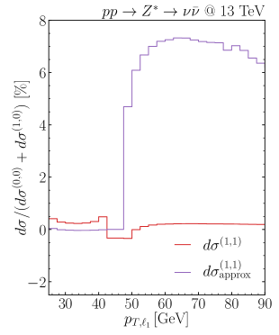
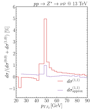
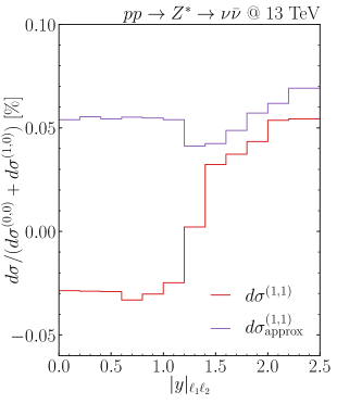
Figure 5: Comparison between the mixed QCD$\otimes$QED corrections (red) and the naive factorisation approximation (purple), for the transverse momentum of the hardest (left) and softer (center) lepton, and the rapidity of the pair (right).

Before going to the summary, it is interesting to compare the size of the mixed QCD$\otimes$QED corrections computed here against the naive approximation in which QCD and QED corrections factorize. Specifically, defining for a given bin

$$d\Delta^{(i,j)}=d\sigma^{(i,j)}/d\sigma^{(0,0)}\,,$$ (33)

the multiplicative approximation to the ${\cal O}(\alpha_{s}\alpha)$ based on NLO QCD and QED predictions is given by the product

$$d\sigma^{(1,1)}_{\text{approx}}=d\sigma^{(0,0)}d\Delta^{(1,0)}d\Delta^{(0,1)}\,.$$ (34)

In figure 5 we present the mixed QCD$\otimes$QED corrections together with the approximation defined by eq. (34), for the transverse momentum of the two leptons and the rapidity of the pair. The results are normalized to the NLO QCD prediction, as in the lower panels of the previous figures. We can observe that, in all cases, the multiplicative approach is a rather poor approximation to the full results. This is in line with the observations made for the total cross section in ref. [31]. The discrepancies, however, can be strongly enhanced at the differential level. This can be seen for instance in the $p_{T,\ell_{1}}>M_{Z}/2$ region, where the exact ${\cal O}(\alpha_{s}\alpha)$ corrections are at the per-mille level, while the factorisation approximation predicts $\sim 7\%$ corrections. The reason for this big discrepancy is the presence of large $K$-factors at NLO (both in QCD and QED), associated to the fact that at LO this region is only populated by events that are away from the $Z$ peak. In the case of the $p_{T,\ell_{2}}$ distribution, we can observe that the multiplicative approach has the wrong sign for $p_{T,\ell_{2}}<M_{Z}/2$ (note that the approximation is not well defined for $p_{T,\ell_{2}}<25$ GeV due to the cut in the hardest lepton), and fails to reproduce the correct size of the corrections around the peak located in $p_{T,\ell_{2}}\sim M_{Z}/2$. Finally, for the rapidity of the lepton pair we can see that the factorisation approximation predicts a rather flat $K$-factor, failing to describe the kinematical dependence of the mixed corrections.

4 Summary

By using the abelianisation techniques [31, 32, 33], in this work we have extended the $q_{T}$-subtraction formalism in order to deal with the case of mixed QCD$\otimes$QED corrections. The method can be applied to the fully exclusive calculation of the ${\cal O}(\alpha_{s}\alpha)$ corrections for the production of a colourless and neutral final state (e.g. $Z$ and Higgs bosons, photons, neutrinos). We have provided all the relevant formulas for its implementation at ${\cal O}(\alpha_{s}\alpha)$. The coefficient functions and the hard virtual coefficients are also of value for transverse momentum resummation and our expressions contain the full dependence on the resummation scale $Q$.

We have applied the method to the production of an off-shell $Z$ boson, and considered its decay into a pair of neutrinos. We presented differential distributions for the final-state leptons at the LHC, and found that the corrections can have a sizeable dependence on the kinematics, and not necessarily following the pattern of the NNLO QCD corrections for instance. The size of the corrections is typically very small and below $1\%$, though it can be enhanced in some particular phase space regions. We note that our predictions are in qualitative agreement with the corresponding results in ref. [36].

We have also compared the mixed QCD$\otimes$QED contribution with the factorisation approximation based on the product of QCD and QED $K$-factors. We have found that this multiplicative approach is in general a bad approximation to the mixed corrections, and the disagreement can be quite extreme for some differential distributions.

As a final remark, it is interesting to point out that recent developments have allowed the application of the $q_{T}$-subtraction method to the production of a heavy-quark pair at NNLO in QCD [48, 49, 50] (see also its related application to NLO EW corrections for massive lepton pair production in ref. [51]). Following similar abelianisation techniques to the ones used in the present paper, the method could be extended to also deal with the mixed QCD$\otimes$QED corrections for the production of a massive charged (colourless) final state.

References

- [1] S. Drell and T.-M. Yan, Massive Lepton Pair Production in Hadron-Hadron Collisions at High-Energies, Phys. Rev. Lett. 25 (1970) 316–320. [Erratum: Phys.Rev.Lett. 25, 902 (1970)].
- [2] G. Altarelli, R. K. Ellis, and G. Martinelli, Large Perturbative Corrections to the Drell-Yan Process in QCD, Nucl. Phys. B157 (1979) 461–497.
- [3] R. Hamberg, W. L. van Neerven, and T. Matsuura, A complete calculation of the order correction to the Drell-Yan factor, Nucl. Phys. B359 (1991) 343–405. [Erratum: Nucl. Phys.B644,403(2002)].
- [4] W. L. van Neerven and E. B. Zijlstra, The corrected Drell-Yan factor in the DIS and MS scheme, Nucl. Phys. B382 (1992) 11–62. [Erratum: Nucl. Phys.B680,513(2004)].
- [5] R. V. Harlander and W. B. Kilgore, Next-to-next-to-leading order Higgs production at hadron colliders, Phys. Rev. Lett. 88 (2002) 201801, [hep-ph/0201206].
- [6] S. Catani, L. Cieri, G. Ferrera, D. de Florian, and M. Grazzini, Vector boson production at hadron colliders: a fully exclusive QCD calculation at NNLO, Phys. Rev. Lett. 103 (2009) 082001, [arXiv:0903.2120].
- [7] K. Melnikov and F. Petriello, The boson production cross section at the LHC through , Phys. Rev. Lett. 96 (2006) 231803, [hep-ph/0603182].
- [8] K. Melnikov and F. Petriello, Electroweak gauge boson production at hadron colliders through , Phys. Rev. D74 (2006) 114017, [hep-ph/0609070].
- [9] R. Gavin, Y. Li, F. Petriello, and S. Quackenbush, FEWZ 2.0: A code for hadronic Z production at next-to-next-to-leading order, Comput. Phys. Commun. 182 (2011) 2388–2403, [arXiv:1011.3540].
- [10] R. Gavin, Y. Li, F. Petriello, and S. Quackenbush, W Physics at the LHC with FEWZ 2.1, Comput. Phys. Commun. 184 (2013) 208–214, [arXiv:1201.5896].
- [11] R. Boughezal, J. M. Campbell, R. K. Ellis, C. Focke, W. Giele, X. Liu, F. Petriello, and C. Williams, Color singlet production at NNLO in MCFM, Eur. Phys. J. C77 (2017), no. 1 7, [arXiv:1605.08011].
- [12] T. Ahmed, N. Mahakhud, M. Rana, and V. Ravindran, Drell-Yan Production at Threshold to Third Order in QCD, Phys. Rev. Lett. 113 (2014), no. 11 112002, [arXiv:1404.0366].
- [13] S. Catani, L. Cieri, D. de Florian, G. Ferrera, and M. Grazzini, Threshold resummation at N3LL accuracy and soft-virtual cross sections at N3LO, Nucl. Phys. B888 (2014) 75–91, [arXiv:1405.4827].
- [14] C. Duhr, F. Dulat, and B. Mistlberger, The Drell-Yan cross section to third order in the strong coupling constant, arXiv:2001.07717.
- [15] S. Dittmaier and M. Krämer, Electroweak radiative corrections to W boson production at hadron colliders, Phys. Rev. D65 (2002) 073007, [hep-ph/0109062].
- [16] U. Baur and D. Wackeroth, Electroweak radiative corrections to beyond the pole approximation, Phys. Rev. D70 (2004) 073015, [hep-ph/0405191].
- [17] C. M. Carloni Calame, G. Montagna, O. Nicrosini, and A. Vicini, Precision electroweak calculation of the charged current Drell-Yan process, JHEP 12 (2006) 016, [hep-ph/0609170].
- [18] U. Baur, O. Brein, W. Hollik, C. Schappacher, and D. Wackeroth, Electroweak radiative corrections to neutral current Drell-Yan processes at hadron colliders, Phys. Rev. D65 (2002) 033007, [hep-ph/0108274].
- [19] U. Baur, S. Keller, and W. K. Sakumoto, QED radiative corrections to boson production and the forward backward asymmetry at hadron colliders, Phys. Rev. D57 (1998) 199–215, [hep-ph/9707301].
- [20] Q.-H. Cao and C. P. Yuan, Combined effect of QCD resummation and QED radiative correction to boson observables at the Tevatron, Phys. Rev. Lett. 93 (2004) 042001, [hep-ph/0401026].
- [21] G. Balossini, G. Montagna, C. M. Carloni Calame, M. Moretti, O. Nicrosini, F. Piccinini, M. Treccani, and A. Vicini, Combination of electroweak and QCD corrections to single W production at the Fermilab Tevatron and the CERN LHC, JHEP 01 (2010) 013, [arXiv:0907.0276].
- [22] N. E. Adam, V. Halyo, S. A. Yost, and W. Zhu, Evaluation of the Theoretical Uncertainties in the Cross Sections at the LHC, JHEP 09 (2008) 133, [arXiv:0808.0758].
- [23] Y. Li and F. Petriello, Combining QCD and electroweak corrections to dilepton production in FEWZ, Phys. Rev. D86 (2012) 094034, [arXiv:1208.5967].
- [24] L. Barze, G. Montagna, P. Nason, O. Nicrosini, F. Piccinini, and A. Vicini, Neutral current Drell-Yan with combined QCD and electroweak corrections in the POWHEG BOX, Eur. Phys. J. C73 (2013), no. 6 2474, [arXiv:1302.4606].
- [25] S. Dittmaier, A. Huss, and C. Schwinn, corrections to Drell-Yan processes in the resonance region, PoS LL2014 (2014) 045, [arXiv:1405.6897].
- [26] S. Dittmaier, A. Huss, and C. Schwinn, Mixed QCD-electroweak corrections to Drell-Yan processes in the resonance region: pole approximation and non-factorizable corrections, Nucl. Phys. B885 (2014) 318–372, [arXiv:1403.3216].
- [27] S. Dittmaier, A. Huss, and C. Schwinn, Dominant mixed QCD-electroweak O(s) corrections to Drell–Yan processes in the resonance region, Nucl. Phys. B904 (2016) 216–252, [arXiv:1511.08016].
- [28] R. Bonciani, F. Buccioni, R. Mondini, and A. Vicini, Double-real corrections at to single gauge boson production, Eur. Phys. J. C77 (2017), no. 3 187, [arXiv:1611.00645].
- [29] R. Bonciani, S. Di Vita, P. Mastrolia, and U. Schubert, Two-Loop Master Integrals for the mixed EW-QCD virtual corrections to Drell-Yan scattering, JHEP 09 (2016) 091, [arXiv:1604.08581].
- [30] R. Bonciani, F. Buccioni, N. Rana, I. Triscari, and A. Vicini, NNLO QCDEW corrections to Z production in the channel, Phys. Rev. D 101 (2020), no. 3 031301, [arXiv:1911.06200].
- [31] D. de Florian, M. Der, and I. Fabre, QCDQED NNLO corrections to Drell Yan production, Phys. Rev. D98 (2018), no. 9 094008, [arXiv:1805.12214].
- [32] D. de Florian, G. F. R. Sborlini, and G. Rodrigo, QED corrections to the Altarelli–Parisi splitting functions, Eur. Phys. J. C76 (2016), no. 5 282, [arXiv:1512.00612].
- [33] D. de Florian, G. F. R. Sborlini, and G. Rodrigo, Two-loop QED corrections to the Altarelli-Parisi splitting functions, JHEP 10 (2016) 056, [arXiv:1606.02887].
- [34] S. Catani and M. Grazzini, An NNLO subtraction formalism in hadron collisions and its application to Higgs boson production at the LHC, Phys. Rev. Lett. 98 (2007) 222002, [hep-ph/0703012].
- [35] S. Catani, L. Cieri, D. de Florian, G. Ferrera, and M. Grazzini, Universality of transverse-momentum resummation and hard factors at the NNLO, Nucl. Phys. B881 (2014) 414–443, [arXiv:1311.1654].
- [36] M. Delto, M. Jaquier, K. Melnikov, and R. Röntsch, Mixed QCDQED corrections to on-shell boson production at the LHC, JHEP 01 (2020) 043, [arXiv:1909.08428].
- [37] F. Caola, K. Melnikov, and R. Röntsch, Nested soft-collinear subtractions in NNLO QCD computations, Eur. Phys. J. C 77 (2017), no. 4 248, [arXiv:1702.01352].
- [38] G. Bozzi, S. Catani, D. de Florian, and M. Grazzini, Transverse-momentum resummation and the spectrum of the Higgs boson at the LHC, Nucl. Phys. B737 (2006) 73–120, [hep-ph/0508068].
- [39] L. Cieri, G. Ferrera, and G. F. Sborlini, Combining QED and QCD transverse-momentum resummation for Z boson production at hadron colliders, JHEP 08 (2018) 165, [arXiv:1805.11948].
- [40] S. Frixione, Z. Kunszt, and A. Signer, Three jet cross-sections to next-to-leading order, Nucl. Phys. B467 (1996) 399–442, [hep-ph/9512328].
- [41] L. J. Dixon, Z. Kunszt, and A. Signer, Helicity amplitudes for production of , , , , or pairs at hadron colliders, Nucl. Phys. B531 (1998) 3–23, [hep-ph/9803250].
- [42] V. Shtabovenko, R. Mertig, and F. Orellana, New Developments in FeynCalc 9.0, Comput. Phys. Commun. 207 (2016) 432–444, [arXiv:1601.01167].
- [43] NNPDF Collaboration, V. Bertone, S. Carrazza, N. P. Hartland, and J. Rojo, Illuminating the photon content of the proton within a global PDF analysis, SciPost Phys. 5 (2018), no. 1 008, [arXiv:1712.07053].
- [44] A. Buckley, J. Ferrando, S. Lloyd, K. Nordström, B. Page, M. Rüfenacht, M. Schönherr, and G. Watt, LHAPDF6: parton density access in the LHC precision era, Eur. Phys. J. C75 (2015) 132, [arXiv:1412.7420].
- [45] M. Grazzini, S. Kallweit, and M. Wiesemann, Fully differential NNLO computations with MATRIX, Eur. Phys. J. C 78 (2018), no. 7 537, [arXiv:1711.06631].
- [46] S. Catani and B. R. Webber, Infrared safe but infinite: Soft gluon divergences inside the physical region, JHEP 10 (1997) 005, [hep-ph/9710333].
- [47] S. Alioli et al., Precision studies of observables in and processes at the LHC, Eur. Phys. J. C77 (2017), no. 5 280, [arXiv:1606.02330].
- [48] R. Bonciani, S. Catani, M. Grazzini, H. Sargsyan, and A. Torre, The subtraction method for top quark production at hadron colliders, Eur. Phys. J. C 75 (2015), no. 12 581, [arXiv:1508.03585].
- [49] S. Catani, S. Devoto, M. Grazzini, S. Kallweit, J. Mazzitelli, and H. Sargsyan, Top-quark pair hadroproduction at next-to-next-to-leading order in QCD, Phys. Rev. D99 (2019), no. 5 051501, [arXiv:1901.04005].
- [50] S. Catani, S. Devoto, M. Grazzini, S. Kallweit, and J. Mazzitelli, Top-quark pair production at the LHC: Fully differential QCD predictions at NNLO, JHEP 07 (2019) 100, [arXiv:1906.06535].
- [51] L. Buonocore, M. Grazzini, and F. Tramontano, The subtraction method: electroweak corrections and power suppressed contributions, Eur. Phys. J. C 80 (2020), no. 3 254, [arXiv:1911.10166].