Almost exact state transfer in a spin chain via pulse control

Abstract

Quantum communication through spin chains has been extensively investigated. In this scenario, state transfer through linearly arranged spins connected by uniform nearest-neighbor couplings qualifies as a natural choice, with minimal control requirements. However, quantum states usually cannot be perfectly transferred through a uniformly coupled chain due to the dispersion of the chain. Here, we propose an effective quantum control technique to realize almost exact state transfer (AEST) in a quantum spin chain. The strategy is to add a leakage elimination operator (LEO) Hamiltonian to the evolution, which implements a sequence of pulse control acting on a perfect state transfer subspace. By using the one-component Feshbach PQ partitioning technique, we obtain the conditions over the required pulses. AEST through a spin chain can then be obtained under a suitable pulse intensity and duration.

I Introduction

Accurate control of a quantum system is crucial for performing quantum tasks Press ; Domenico , such as adiabatic quantum computing Farhi:01 ; Albash , quantum thermodynamic processes Kieu:04 ; Hu:19 , stable energy transfer in quantum batteries Santos:19 ; Santos:19-2 ; Rosa:19 , speedup of quantum circuits Nakahara ; Santos:15 , acceleration of chemical reactions Prezhdo , among others. In general, quantum control techniques are employed to constrain a quantum evolution towards a target state or a target path Wunotes . For example, in adiabatic quantum computation, the system is slowly evolved to be maintained, with high probability, at the lowest-energy instantaneous eigenstate. In order to speed up the adiabatic dynamics, shortcuts to adiabaticity can be implemented through counter-diabatic control fields Demirplak:03 ; Demirplak:05 ; Berry:09 ; Torrontegui:13 . Counter-diabatic transitionless driving has been extensively realized. In particular, it has been applied to speed up stimulated Raman adiabatic passage in a solid-state lambda system zhou and in cold atoms Du . More recently, counter-diabatic fields have also been used to yield energy-optimal shortcuts to adiabaticity in trapped ions Hu:18 and to accelerate quantum gates in nuclear magnetic resonance Santos:20 .

In the context of open system control, adiabatic speedup has recently been implemented in a non-Markovian evolution through an effective set of pulses on the system Wang20182 . In this scenario, a relevant set of techniques is provided by dynamical decoupling control, such as Bang-Bang (B-B) Viola ; Vitali and LEO control Wu02 . B-b control requires unbounded fast and strong pulses while LEOs are introduced to counteract leakage from a subsystem to the rest of a multilevel Hilbert space Wu02 ; Byrd05 ; Campo13 ; Campo11 . In this case, only finite pulse intensity and time interval are required, since the effectiveness of the control only depends on the integral of the pulse sequence in the time domain Jing2014 . By adding a LEO Hamiltonian to the adiabatic frame, the transitions between different instantaneous eigenstates are restrained Wang2018 and the system undergoes the adiabatic passage. For a two-level system, the LEO Hamiltonian in the adiabatic frame is equivalent to adding a global pulse on the Hamiltonian in the experimental frame Wang2018 . This can be extended to the open system realm, where inverse engineering control can be applied and a time-dependent Hamiltonian can be derived in order to guide the system to attain an arbitrary target state at a predefined time Wu2013 .

Quantum information processing tasks often require the active transmission of a quantum state over relatively short distances Kimble . Spin chains can serve as a suitable communication channel in these cases. In fact, reliable quantum state transfer through a spin chain has been extensively studied Bose ; Wu20091 ; Yung ; Wu20092 ; Wang2009 . It was Bose who first suggested the use of an unmodulated spin chain as a channel for quantum information transfer Bose . However, in most situations, this method does not allow for a perfect state transfer. The fidelity will decrease quickly with increasing length of the chain. Thus, a number of schemes have been proposed to improve the transmission fidelity, such as by using a single local on-off switch actuator Schirmer , a suitable sequence of two-qubit gates at the end of the chain Burgarth , optimal control to an external parabolic magnetic field Murphy , and optimal state encoding Wang2009 . More recently, the fastest transmission speed while maintaining high fidelities has been achieved by reinforcement learning in a spin chain Yun2018 .

The experimental platforms to realize spin systems include trapped ions  Zeiher , ultracold atoms in optical lattices Grusdt , quantum dots Veldhorst , etc. For some physical systems, such as ultracold atoms in optical lattices, the required couplings between different sites can be created Wang2013 . Engineering special couplings between neighbor sites can realize perfect state transfer (PST) Christandl or near PST Wojcik ; Oh ; Wang2013 . Then, a PST or near PST trajectory can be obtained. For some other systems, it might be inconvenient to create the designed couplings. Here, we aim at creating a LEO Hamiltonian by using either PST or near PST trajectories to realize almost exact state transfer (AEST), being able to drive quantum communication through a set of pulses over a uniform spin chain. By using the Feshbach PQ partition technique Feshbach , we obtain the conditions to be obeyed by the required pulses, which are provided by the pulse intensity, pulse interval and total evolution time. Throughout this analysis, we will consider various pulse patterns, including rectangular pulses and sine function. Especially, we use the so-called zero-energy-change pulse, in which the total integration is zero in one period. In addition, we show that the pulse control scheme used in Refs Wang20182 ; Wang2018 to speed up adiabatic processes can be generalized to the quantum communication domain.

II Construction of the LEO Hamiltonian

Define a complete orthonormal basis $\left|\Psi_{n}(0)\right\rangle$, $\langle\Psi_{m}(0)|\Psi_{n}(0)\rangle=\delta_{mn}$. Suppose there exists a complete orthonormal basis $\left|\Psi_{n}(t)\right\rangle$, $\langle\Psi_{m}(t)|\Psi_{n}(t)\rangle=\delta_{mn}(t)$, and a one-to-one correspondence between the states $|\Psi_{n}(0)\rangle$ and $|\Psi_{n}(t)\rangle$. For example, $\left|\Psi_{n}(t)\right\rangle$ could be the instantaneous eigenstates of a time-dependent Hamiltonian $H(t)$. Our target problem is to drive the system along the $\left|\Psi_{1}(t)\right\rangle$ passage within a finite time with high probability.

The LEO Hamiltonian can be constructed as

$$H_{LEO}(t)=c(t)\left|\Psi_{1}(t)\right\rangle\left\langle\Psi_{1}(t)\right|,$$ (1)

where $c(t)$ is the external control function that describes a sequence of control pulses. LEOs can be used to reduce errors from an encoded subspace $\left|\Psi_{1}(t)\right\rangle\left\langle\Psi_{1}(t)\right|$ to the rest of the system’s subspace, whether the pulses are ideal Feshbach or non-ideal Jing2015PRL ; Licheng . The total Hamiltonian is then

$$H(t)=H_{0}+H_{LEO}(t),$$ (2)

where $H_{0}$ is the original Hamiltonian of the system, e.g., the local Hamiltonian of a uniform spin chain.

III One-component dynamical equation

Given a time-dependent Hamiltonian $H(t)$, the system dynamics is governed by its corresponding Schrödinger equation

$$i|\dot{\Psi}(t)\rangle=H(t)\left|\Psi(t)\right\rangle,$$ (3)

with the dot symbol denoting time derivative and $\hbar=1$ throughout the paper. The state vector $\left|\Psi(t)\right\rangle$ can be expanded in terms of the time-dependent basis $\{\left|\Psi_{n}(t)\right\rangle\}$, which reads

$$\left|\Psi(t)\right\rangle=\sum\nolimits_{n}a_{n}(t)\left|\Psi_{n}(t)\right\rangle,$$ (4)

where $a_{n}(t)$ denotes a complex amplitude probability. Substituting Eq. (4) in Eq. (3), we obtain

$$i\dot{a}_{n}=\sum\limits_{m}[\langle\Psi_{n}|H(t)|\Psi_{m}\rangle-i\langle\Psi_{n}|\dot{\Psi}_{m}\rangle]a_{m}.$$ (5)

Eq. (5) can be rearranged in a vector form, with the left-hand-side written as $\left|\Psi(t)\right\rangle=[a_{1},a_{2},...]^{{}^{\prime}}$ and the right-hand-side given in terms of the effective Hamiltonian $H_{n,m}(t)=\langle\Psi_{n}|H(t)|\Psi_{m}\rangle-i\langle\Psi_{n}{|\dot{\Psi}_{m}\rangle}$. To trace the footprint of $\left|\Psi_{1}(t)\right\rangle$, one needs to find an exact one-component dynamical equation for $a_{1}$. Feshbach P-Q partitioning technique provides an effective approach to solve this problem (see, e.g., Ref. Jing:16 ).

Using the $PQ$ partitioning, the $n$-dimensional state vector $\left|\Psi(t)\right\rangle$ can be divided into two parts: a one-dimensional vector of interest, $P(t)$, and the rest, an $(n-1)$-dimensional vector $Q(t)$. The Hamiltonian can be split into three contributions $H(t)=H_{P}(t)+H_{Q}(t)+H_{L}(t)$, with $H_{P}(t)$ and $H_{Q}(t)$ acting on the subspaces defined by $P(t)$ and $Q(t)$, respectively, and $H_{L}(t)$ representing the remaining off-diagonal contributions. The state vector $\left|\Psi(t)\right\rangle$ and the matrix representation of the Hamiltonian $H(t)$ can then be written as

$$|\Psi(t)\rangle=\left[\begin{array}[]{c}P(t)\\ Q(t)\end{array}\right],H(t)=\left[\begin{array}[]{cc}h(t)&R(t)\\ W(t)&D(t)\end{array}\right],$$ (6)

where the $1\times 1$ matrix $h(t)$ and $(n-1)\times(n-1)$ matrix $D(t)$ are the self-Hamiltonians in the subspaces of $P(t)$ and $Q(t)$, respectively, while the off-diagonal contributions $R(t)$ and $W(t)$ denote $1\times(n-1)$ and $(n-1)\times 1$ matrices, respectively.

Let $p(t)=\exp[-i\int\nolimits_{0}^{t}h(s^{\prime})ds^{\prime}]P(t)$. In the selected one-dimensional subspace, the projected Schrödinger equation (see, e.g., Ref. (Jing:16 ) will imply that $p(t)$ satisfies

$$\dot{p}(t)=\int\nolimits_{0}^{t}\tilde{g}(t,s)p(s)ds,$$ (7)

where $\tilde{g}(t,s)$ is the propagator given by $\tilde{g}(t,s)=-g(t,s)\exp[-i\int\nolimits_{s}^{t}h(s^{\prime})ds^{\prime}]$, with $g(t,s)=R(t)G(t,s)W(s)$, $G(t,s)=\Gamma_{\leftarrow}\{\exp[-i\int\nolimits_{s}^{t}D(s^{\prime}){ds^{\prime}}]\}$, and $\Gamma_{\leftarrow}$ denoting the time-ordering operator. Specifically,

$$\dot{p}(t)=-\int\nolimits_{0}^{t}g(t,s)e^{-i\int\nolimits_{s}^{t}h(s^{\prime})ds^{\prime}}p(s)ds.$$ (8)

IV Pulse control conditions

If $\dot{p}(t)=0$, the system will be kept in the subspace $\left|\Psi_{1}(t)\right\rangle\left\langle\Psi_{1}(t)\right|$. By adding a control Hamiltonian $H_{LEO}(t)$ whose control strength is large enough, we have that $c(s)$ will dominate the exponential term for $h(s)$ in Eq. (8). Moreover, a strong control function $c(s)$ will ensure that $g(t,s)p(s)$ varies slowly compared with $\exp[-i\int\nolimits_{s}^{t}c(s^{\prime})ds^{\prime}]$. Therefore, Eq. (8) can be simplified to

$$\int\nolimits_{0}^{\tau}ds\exp\left[-i\int\nolimits_{0}^{s}c(s^{{\prime}})ds^{{\prime}}\right]=0,$$ (9)

where $\tau$ corresponds to a single control time interval.

Here as an example we consider two types of periodic control: rectangular pulses and sine function. First for rectangular pulses, the control function can be taken as

$$c(t)=\{\begin{array}[]{c}I,\\ -I,\end{array}\begin{array}[]{l}n\tau<t<(n+1)\tau,\,\text{for }n\text{ even},\\ \text{otherwise,}\end{array}$$ (10)

where $I$ represents the control strength and $\tau$ is the running time for applying a single (either positive or negative) pulse. Notice that $c(t)$ can be realized by a sequence of fast pulses through an arbitrary physical setup. Inserting Eq. (10) into Eq. (9), we obtain Paval2016

$$I\tau=2\pi m,\,\text{for }m=1,2,3,....$$ (11)

If the rectangular control pulses satisfy the above conditions, the transition from the state $\left|\Psi_{1}(t)\right\rangle$ to other states will be restrained. For sine function, we have

$$c(t)=I\sin(\omega t).$$ (12)

Eq. (9) is equivalent to

$$\int\nolimits_{0}^{\tau}ds\exp[\frac{iI}{\omega}\cos(\omega s)]=0.$$ (13)

Let $\omega\tau=\pi$. Then, equation above becomes

$$J_{0}(I\tau/\pi)=0,$$ (14)

where $J_{0}(x)$ is the zero order Bessel function of the first kind.

V AEST under LEO control in spin chains

Now we will show that, by choosing an appropriate LEO Hamiltonian, AEST can be realized with high fidelity. We consider the communication channel as a one-dimensional XY spin chain, whose Hamiltonian reads

$$H=\sum\limits_{i=1}^{N-1}J_{i,i+1}(\sigma_{i}^{x}\sigma_{i+1}^{x}+\sigma_{i}^{y}\sigma_{i+1}^{y}),$$ (15)

where $J_{i,i+1}$ is coupling constant between nearest-neighbor sites and $\sigma^{k}_{i}(k=x,y)$ are Pauli operators acting on the spin at site $i$. For a uniformly coupled chain, the Hamiltonian $H$ can be represented by $H_{UNI}$, with $J_{i,i+1}=J$ is a constant. For simplicity, we take $J=1$.

As an example, we can transfer the state $\left|1\right\rangle$ from one end of the chain to the other end. Initially all the other spins are in the state $\left|0\right\rangle.$ The initial state of the system is then $\left|10..0\right\rangle=\left|\Psi_{1}\right\rangle.$ Here we use $\left|\Psi_{n}\right\rangle$ to denote that the nth spin is in the up state while all the other spins are in the down state. Define the fidelity as $F(t)=\sqrt{\left\langle\Psi_{n}\right|\rho(t)\left|\Psi_{n}\right\rangle}$, where $\rho(t)$ is the instantaneous density operator of the system. The fidelity will decrease quickly by increasing the length $N$ of the chain in a uniform chain Bose .

Our aim is then to provide a robust AEST scheme through a uniform chain by adding a LEO Hamiltonian. This will be achieved by considering two types of spin chain Hamiltonians in Eq. (15): (i) PST couplings $J_{i,i+1}=\sqrt{i(N-i)}$ ($H_{PST}$); (ii) weak couplings $J_{1,2}=J_{N-1,N}=J_{0}$ and $J_{i,i+1}=J$ elsewhere, with $J_{0}\ll J$ ($H_{WC}$). By directly realizing state transfer through the XY spin chain driven by PST couplings, at time $t=k\pi/2$ ($k$ is an integer), we have that PST occurs, with the state $\left|1\right\rangle$ being perfectly transferred from the first site to the last Christandl . Similarly, for the spin chain driven by weak couplings, AEST can also be realized Wojcik ; Oh ; Wang2013 .

In order to implement AEST with LEO control, we take the complete orthonormal basis as

$$\left|\Psi_{n}(t)\right\rangle=V(t)\left|\Psi_{n}\right\rangle,$$ (16)

where $V(t)=\exp(-iH_{j}t)$, $(j=PST$ or $WC)$. Clearly $\left\langle\Psi_{m}(t)\mid\Psi_{n}(t)\right\rangle=\delta_{mn}$ and we will satisfy the one-to-one relationship between $|\Psi_{n}(t)\rangle$ and $\left|\Psi_{n}\right\rangle$. In what follows, we will consider the AEST in a uniform chain.

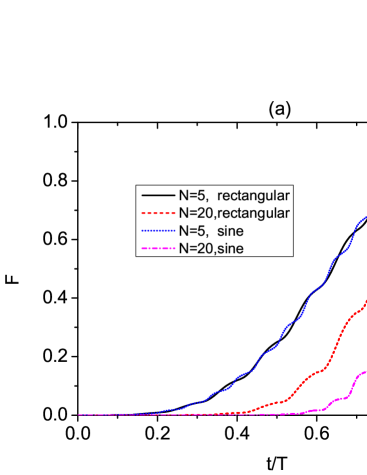
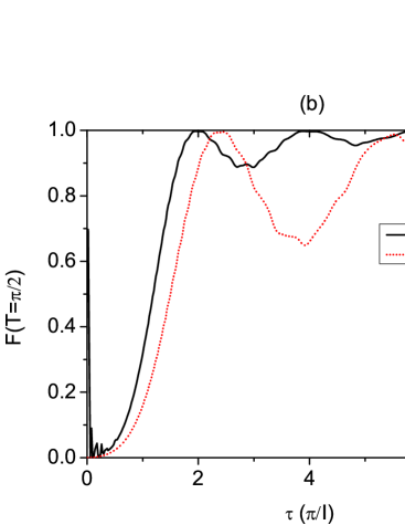
Figure 1: Fidelity for AEST under LEO control with PST couplings. We adopted $T=\pi/2$. (a) Fidelity $F$ as a function of the normalized time $t/T$ for either rectangular pulses or sine function. For rectangular pulses, we used $I=40$ and $\tau=\pi/20$. For the sinusoidal case, we used $I=80$ and $\tau=2.405\pi/80$. (b) Fidelity $F(T=\pi/2)$ as a function of the control time interval $\tau$ for either rectangular pulses or sine function. For both cases, we used $I=50$ and $N=10$. Note that the peak of $F$ occurs at $I\tau=2m\pi,m=1,2,3,...$ for rectangular pulses and $I\tau=x\pi$, with $x=2.405,5.520,...$, for sine function. The value of $x$ is the zero point of the Bessel function of the first kind $J_{0}(x)$.

VI Discussion

First, let us take PST couplings in Eq. (16), namely, $V(t)=\exp[-iH_{PST}t]$. We then plot the fidelity $F$ as a function of the normalized time $t/T$ in Fig. 1(a), where the density operator is exactly obtained through the solution of the time-dependent Schödinger equation. For either rectangular pulses or sine function, the total evolution time is taken as $T=\pi/2$. For rectangular pulses, we take the amplitude as $I=40$ and the time period as $\tau=\pi/20$ according to Eq. (11), while for sine function, we take $I=80$ and $\tau=2.405\pi/80$, according to Eq. (14). We analyze chains with lengths $N=5,20$. Notice that, from $t=0$ to $t=T$, $F$ increases from zero to nearly unity for both kinds of pulses and independently of $N$. Then, at time $t=T$, AEST can be realized with high fidelity.

In Fig. 1(b) we plot $F(t=\pi/2)$ as a function of $\tau$. The fidelity $F$ initially increases as we increase $\tau$ and then it shows an oscillating behavior. These two curves have peaks for certain periods $\tau$. The parameters are set as $T=\pi/2$, $I=50$, and $N=10$. For rectangular pulses, the peaks correspond to $\tau=(2,4,6,8,...)\pi/I$. For sine function, they are $\tau=x\pi/I,x=2.405,5.520,8.654,...$. It is worth noting that the values for $\tau$ satisfy Eqs. (11) and (14), in agreement with the theoretical prediction by the Feshbach P-Q partitioning technique.

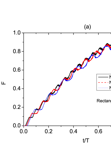
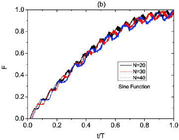
Figure 2: Fidelity for AEST under LEO control with WC couplings. We adopted $T=210\pi$. The fidelity $F$ is plotted as a function of the normalized time $t/T$ for different kinds of pulses and chain sizes $N$. (a) Rectangular pulses. We used $I=60$ and $\tau=\pi/30$. (b) Sine function. We used $I=120$ and $\tau=2.405\pi/120$.

Let us now suppose the LEO control is generated by the weak coupling Hamiltonian $V(t)=\exp[-iH_{WC}t]$. In Figs. 2(a) and (b), we then plot the fidelity $F$ versus the normalized time $t/T$ for either rectangular pulses or sine function. We consider chains with lengths $N=20,30,40$. The evolution time is $T=210\pi$. For both kinds of pulses, AEST ($F=0.999$) can be obtained at time $T$ by effective pulse control. For rectangular pulses, we used $I=60$ and $\tau=\pi/30$, which satisfies Eq (11). For sine function, we used $I=120$ and $\tau=2.405\pi/I$. This is the first zero value of the Bessel function of the first kind $J_{0}(x)$. Notice that Fig. 2 again illustrates the effectiveness of the pulse control scheme, with the only requirement being the adoption of a LEO Hamiltonian implementing PST or near PST passage.

Until now, the pulses we used are finite and continuous in the above discussion, i.e., at any time the pulses are present on the chain even though they alternate their directions. This can be regarded as a limit case. The opposite (second) limit is to utilize a discontinuous and strong pulse sequence, such as B-B kicks (pulses) $c(t)=\pi\sum_{i}(-1)^{i}\delta(t-\tau_{i})$ Paval2016 . As in the first limit case, again we can use the zero-energy-change pulse. Two consecutive B-B pulses take positive and negative values respectively. We point out that this case is equivalent to the case that all the negative pulses become positive Paval2016 . In the numerical calculation we use rectangular pulses and LEO Hamiltonian with PST coupling to simulate the $\delta$ function pulse. Again the total evolution time is taken as $T=\pi/2$. For a continuous pulse, we take $I=120$ and $\tau=\pi/120$. Now we use $c(t)=50I$, for $n\tau<t<(n+1/50)\tau$ (odd $n$), $c(t)=-50I$ for $n\tau<t<(n+1/50)\tau$ (even $n$), and $c(t)=0$, otherwise. Note that, for the above choice of $c(t)$, the integration still satisfies $\int_{0}^{\tau}c(s)ds=\pi$ in a time interval $\tau$. Even though $I\gg J$, $c(t)$ oscillates in the range $[-I,I]$. It is worthy emphasizing that the second limit is experimentally feasible, e.g. using dynamical-decoupling techniques to moderate the dephasing effects of low-frequency noise on a superconducting qubit David . In Fig. 3, we plot the fidelity $F$ versus the normalized time $t/T$ for the simulated B-B pulses. We consider chains with lengths $N=10,20,30,40$. The results again show that the simulated B-B pulses are effective to realize AEST in a uniform chain.

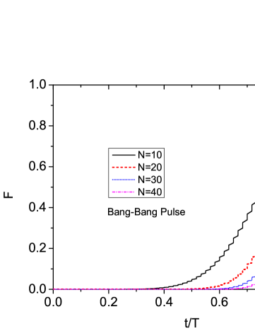
Figure 3: Fidelity for AEST under the B-B pulse control with PST couplings for different $N$. We adopted $T=\pi/2$. The pulses are present at $\tau/50$ and otherwise absent in a time interval $\tau=\pi/120$. The integration in $\tau$ satisfies $I\tau=\pi$.

VII Conclusions

High fidelity quantum state transfer through spin chains is a powerful tool for performing short-distance quantum communication in a quantum network. We have introduced an effective pulse control scheme to realize AEST in a uniform chain by adding a LEO Hamiltonian to the evolution. The LEO Hamiltonian can be represented by a sequence of pulses acting on (near) PST subspaces. By using the Feshbach PQ partitioning technique, we obtained the conditions over the pulses to allow AEST, which prevent transitions from the target state to other undesired states. As an example, we illustrated two kinds of pulses in the XY spin chain: rectangular pulses and sine function. For both pulses, the relations of the pulse intensity and its duration is obtained. Numerical analysis explicitly shows that, once the pulse satisfies the required condition, AEST can be successfully obtained in a uniform chain setup.

VIII Acknowledgements

This material is based upon work supported by NSFC (Grant Nos. 11475160, 61575180,11575071) and the Natural Science Foundation of Shandong Province (Nos. ZR2014AM023, ZR2014AQ026). M.S.S. is supported by Conselho Nacional de Desenvolvimento Científico e Tecnológico (CNPq-Brazil). M.S.S. also acknowledges financial support in part by the Coordenação de Aperfeiçoamento de Pessoal de Nível Superior - Brasil (CAPES) (Finance Code 001) and by the Brazilian National Institute for Science and Technology of Quantum Information [CNPq INCT-IQ (465469/2014-0)]. L.-A.W. is supported by the Basque Country Government (Grant No. IT986-16) and PGC2018-101355- B-I00 (MCIU/AEI/FEDER,UE).

References

- (1) D. Press, T. D. Ladd, B. Zhang and Y. Yamamoto, Nature 456, 218 (2008).
- (2) D. D’Alessandro, Introduction to Quantum Control and Dynamics (Chapman and Hall/CRC, New York, 2007).
- (3) E. Farhi, J. Goldstone, S. Gutmann, J. Lapan, A. Lundgren, and D. Preda, Science 292, 472 (2001).
- (4) T. Albash and D. A. Lidar, Rev. Mod. Phys. 90, 015002 (2018).
- (5) T. D. Kieu, Phys. Rev. Lett. 93, 140403 (2004).
- (6) C.-K. Hu, A. C. Santos, J.-M. Cui et al., e-print arXiv:1902.01145 (2019).
- (7) A. C. Santos, B. Çakmak, S. Campbell, and N. T. Zinner, Phys. Rev. E 100, 032107 (2019).
- (8) A. C. Santos, A. Saguia, and M. S. Sarandy, e-print arXiv:1912.03675 (2019).
- (9) D. Rosa, D. Rossini, G. M. Andolina, M. Polini, and M. Carrega, e-print arXiv:1912.07247 (2019).
- (10) M. Nakahara, Y. Kondo, K. Hata, and S. Tanimura, Phys. Rev. A 70, 052319 (2004).
- (11) A. C. Santos and M. S. Sarandy, Sci. Rep. 5, 15775 (2015).
- (12) O. V. Prezhdo, Phys. Rev. Lett. 85, 4413 (2000).
-
(13)
L.-A. Wu, http://www.authorstream.com/Presentation
/james405702-2822542-universalleo/ - (14) M. Demirplak and S. A. Rice, J. Phys. Chem. A 107, 9937 (2003).
- (15) M. Demirplak and S. A. Rice, J. Phys. Chem. B 109, 6838 (2005).
- (16) M. V. Berry, J. Phys. A: Math. Theor. 42, 365303 (2009).
- (17) E. Torrontegui, S. Ibáñez, S. Martínez-Garaot et al., Adv. Atom. Mol. Opt. Phys. 62, 117 (2013).
- (18) B. B. Zhou, A. Baksic, H. Ribeiro et al., Nature Phys. 13, 330 (2017).
- (19) Y.-X. Du, Z.-T. Liang, Y.-C. Li et al., Nature Commun. 7, 12479 (2016).
- (20) C.-K. Hu, J.-M. Cui, A. C. Santos et al., Opt. Lett. 43, 3136 (2018).
- (21) A. C. Santos, A. Nicotina, A. M. de Souza, R. S. Sarthour, I. S. Oliveira, and M. S. Sarandy, EPL 129, 30008 (2020).
- (22) Z.-M. Wang, D.-W. Luo, M. S. Byrd, L.-A. Wu, T. Yu and B. Shao, Phys. Rev. A 98, 062118 (2018).
- (23) L.Viola, E. Knill, and S. Lloyd, Phys. Rev. Lett. 82, 2417 (1999).
- (24) D. Vitali and P. Tombesi, Phys. Rev. A 59, 4178 (1999).
- (25) L.-A. Wu, M. S. Byrd, and D. A. Lidar, Phys. Rev. Lett. 89, 127901 (2002).
- (26) M. S. Byrd, D. A. Lidar, L.-A. Wu, and P. Zanardi, Phys. Rev. A 71, 052301 (2005).
- (27) A. del Campo, I. L. Egusquiza, M. B. Plenio, and S. F. Huelga, Phys. Rev. Lett. 110, 050403 (2013).
- (28) A. del Campo, Phys. Rev. A 84, 031606 (2011).
- (29) J. Jing, L.-A. Wu, T. Yu, J. Q. You, Z.-M. Wang, and L. Garcia, Phys. Rev. A 89, 032110 (2014).
- (30) Z.-M. Wang, M. S. Byrd, J. Jing, and L.-A. Wu, Phys. Rev. A 93, 062338 (2018).
- (31) J. Jing, L.-A. Wu, M. S. Sarandy, and J. G. Muga, Phys. Rev. A 88, 053422 (2013).
- (32) H. J. Kimble, Nature, 453, 1023 (2008).
- (33) S. Bose, Phys. Rev. Lett. 91, 207901 (2003).
- (34) L.-A. Wu, A. Miranowicz, X. B. Wang, Y.-x. Liu, and F. Nori, Phys. Rev. A 80, 012332 (2009).
- (35) H. Yung, Phys. Rev. A 74, 030303 (R) (2006).
- (36) L.-A. Wu, Y.-x. Liu, and F. Nori, Phys. Rev. A 80, 042315 (2009).
- (37) Z.-M. Wang, C. A. Bishop, M. S. Byrd, B. Shao, and J. Zou, Phys. Rev. A 80, 022330 (2009).
- (38) S. G. Schirmer and P. J. Pemberton-Ross, Phys. Rev. A 80, 030301 (2009).
- (39) D. Burgarth, V. Giovannetti, and S. Bose, Phys. Rev. A 75, 062327 (2007).
- (40) M. l Murphy, S. Montangero, V. Giovannetti, and T. Calarco, Phys. Rev. A 82, 022318 (2010).
- (41) X.-M. Zhang, Z.-W. Cui, X. Wang, and M.-H. Yung, Phys. Rev. A 97, 052333 (2018).
- (42) J. Zeiher, J.-y. Choi, A. Rubio-Abadal, T. Pohl, R. v. Bijnen, I. Bloch, and C. Gross, Phys. Rev. X 7, 041063 (2017).
- (43) F. Grusdt, T. Li, I. Bloch, and E. Demler, Phys. Rev. A 95, 063617 (2017).
- (44) M. Veldhorst, C. Yang, J. Hwang et al., Nature 526, 410 (2015).
- (45) Z.-M. Wang, L.-A. Wu, M. Modugno, W. Yao and B. Shao, Sci. Rep. 3, 3128 (2013).
- (46) M. Christandl, N. Datta, A. Ekert, and A. J. Landahl, Phys. Rev. Lett. 92, 187902 (2004).
- (47) A. Wójcik, T. Luczak, P. Kurzyński, A. Grudka, T. Gdala, and M. Bednarska, Phys. Rev. A 72, 034303 (2005).
- (48) S. Oh, L.-A. Wu, Y.-P. Shim, J. Fei, M. Friesen, and X. Hu, Phys. Rev. A 84, 022330 (2011),
- (49) L.-A. Wu, G. Kurizki, and P. Brumer, Phys. Rev. Lett. 102, 080405 (2009).
- (50) J. Jing, L.-A. Wu, M. Byrd, J. Q. You, T. Yu, and Z.-M. Wang, Phys. Rev. Lett. 114, 190502 (2015).
- (51) L.-C. Zhang, F. H. Ren, R.-H. He et al., EPL 125, 10010 (2019).
- (52) J. Jing, M. S. Sarandy, D. A. Lidar, D.-W. Luo, L.-A. Wu, Phys. Rev. A 94, 042131 (2016).
- (53) P. V. Pyshkin, D.-W. Luo, J. Jing, J. Q. You, and L.-A. Wu, Sci. Rep. 6, 37781 (2016).
- (54) J. Bylander, S. Gustavsson, F. Yan et al., Nature Phys. 7, 565 (2011).