Global sensitivity analysis for stochastic simulators based on generalized lambda surrogate models

Abstract

Global sensitivity analysis aims at quantifying the impact of input variability onto the variation of the response of a computational model. It has been widely applied to deterministic simulators, for which a set of input parameters has a unique corresponding output value. Stochastic simulators, however, have intrinsic randomness due to their use of (pseudo)random numbers, so they give different results when run twice with the same input parameters but non-common random numbers. Due to this random nature, conventional Sobol’ indices, used in global sensitivity analysis, can be extended to stochastic simulators in different ways. In this paper, we discuss three possible extensions and focus on those that depend only on the statistical dependence between input and output. This choice ignores the detailed data generating process involving the internal randomness, and can thus be applied to a wider class of problems. We propose to use the generalized lambda model to emulate the response distribution of stochastic simulators. Such a surrogate can be constructed without the need for replications. The proposed method is applied to three examples including two case studies in finance and epidemiology. The results confirm the convergence of the approach for estimating the sensitivity indices even with the presence of strong heteroskedasticity and small signal-to-noise ratio.

1 Introduction

Computational models, a.k.a. simulators, have been extensively used to represent physical phenomena and engineering systems. They can help assess the reliability, control the risk and optimize the behavior of complex systems early at the design stage. Conventional simulators are usually deterministic, in the sense that repeated model evaluations with the same input parameters yield the same value of the output. In contrast, several runs of a stochastic simulator for a given set of input parameters provide different results. More precisely, the output of a stochastic simulator is a random variable following an unknown probability distribution. Hence, each model evaluation with the same input values generates a realization of the random variable. Mathematically, a stochastic simulator can be defined by

$$\begin{split}{\mathcal{M}}_{s}:{\mathcal{D}}_{\bm{X}}\times\Omega&\rightarrow{\mathbb{R}}\\ (\bm{x},\omega)&\mapsto{\mathcal{M}}_{s}(\bm{x},\bm{Z}(\omega)),\end{split}$$ (1)

where $\bm{x}$ is the input vector that belongs to the input space ${\mathcal{D}}_{\bm{X}}$, and $\Omega$ denotes the probability space that represents the stochasticity. The intrinsic randomness is due to the fact that some latent variables $\bm{Z}(\omega)$ inside the model are not explicitly considered as a part of the input variables: given a fixed input value $\bm{x}_{0}$, the output of the simulator is a random variable.

In this respect, we can consider a stochastic simulator as a random field indexed by the parameters $\bm{x}\in{\mathcal{D}}_{\bm{X}}$ [1]. For a given realization of the latent variables $\bm{z}_{0}$, the simulator becomes a deterministic function of $\bm{x}$. This is realized in practice by initializing the random seed to the same value before running the simulator for different $\bm{x}$’ s, a trick known as common random numbers. The (classical) functions $\bm{x}\mapsto{\mathcal{M}}_{s}(\bm{x},\bm{z}_{0})$ will be called trajectories in this paper. One particular trajectory corresponds to one particular value $\bm{z}_{0}$.

In contrast, for a given $\bm{x}_{0}\in{\mathcal{D}}_{\bm{X}}$, the output of the stochastic simulator is a random variable. Its distribution can be obtained by repeatedly running the simulator with $\bm{x}_{0}$, yet different realizations of the latent variables called replications.

Stochastic simulators are ubiquitous in modern engineering, finance and medical sciences. Typical examples include stochastic differential equations (e.g., financial models [2]) and agent-based models (e.g., epidemiological models [3]). To a certain extent, physical experiments can also be considered as stochastic models, because we may not be able to measure and consider all the relevant variables that can uniquely determine the experimental conditions.

In practice, the input variables may be affected by uncertainty due to noisy measurements, expert judgment or lack of knowledge. Therefore, they are modeled as random variables and grouped into a random vector $\bm{X}=\left(X_{1},X_{2},\ldots,X_{M}\right)$, which is characterized by a joint distribution $f_{\bm{X}}$. Quantification of the contribution of input variability to the output uncertainty is a major task in sensitivity analysis [4]. It allows us to identify the most important set of input variables that dominate the output variability and also to figure out non-influential variables. This information provides more insights into the simulator and can be further used for model calibrations and decision making [5].

A large number of methods have been successfully developed to perform sensitivity analysis in the context of deterministic simulators [4, 6, 7]. Among others, the variance-based sensitivity analysis, also referred to as Sobol’ indices [8], is one of the most popular approaches, which relies on the analysis of variance. Several extensions of Sobol’ indices to stochastic simulators can be found in the literature, depending on the treatment of the intrinsic randomness. It is worth emphasizing that the overall uncertainty now consists of two parts, namely the inherent stochasticity in the latent variables and the uncertainty in the input parameters $\bm{X}$. Iooss and Ribatet [9] include the latent variables as a part of the input, which results in a natural extension of the classical Sobol’ indices to stochastic simulators. Hart et al. [10] and Jimenez et al. [11] define the Sobol’ indices as functions of the latent variables which, as a consequence, become random variables whose statistical properties can be studied. Recently, Azzi et al. [12] propose to represent the intrinsic randomness by the entropy of the response distribution and to calculate the classical Sobol’ indices on the latter. All in all, relatively little attention has been devoted to sensitivity analysis for stochastic simulators.

Sensitivity analysis usually requires a large number of model evaluations for different realizations of the input vector. Due to the intrinsic randomness of stochastic simulators, an additional layer of stochasticity comes on top of the input uncertainty, which requires repeated runs with the same input parameters to fully characterize the model response. As a consequence, such analyses become intractable when the simulator is expensive to evaluate. To alleviate the computational burden, surrogate models can be constructed to mimic the original numerical model at a smaller computational cost. Large efforts have been dedicated to emulating the mean and variance function of stochastic simulators [13, 14, 15]. These two functions provide only the first two moments of the response distribution and are mostly used to estimate the Sobol’ indices proposed in [9]. In recent papers [16, 17], we developed a novel surrogate model, called generalized lambda model (GLaM), to emulate the whole response distribution of stochastic simulators. This model uses generalized lambda distributions (GLD) [18] to flexibly approximate the response distribution, while the distribution parameters cast as functions of the inputs are approximated through polynomial chaos expansions (PCE) [19].

Based on these premises, the goal of this paper is to establish a clear framework to carry out global sensitivity analysis for stochastic simulators, and to propose efficient computational approaches based on GLaM stochastic emulators. Therefore, the original contributions of this paper are two-fold. On the one hand, we give a thorough review of the current development of global sensitivity analysis for stochastic simulators. We point out the nature and the properties of different extensions of Sobol’ indices, which provides a general guideline to their usage. On the other hand, we present a unified framework based on generalized lambda models to calculate a whole variety of global sensitivity indices using this single surrogate.

The paper is organized as follows. First, we review three extensions of Sobol’ indices to stochastic simulators in Section 2. In Section 3, we present the framework of GLaMs [16]. There, we recap the fitting procedure proposed in [17], where it is emphasized that there is no need for replicated runs. Then, we discuss the use of GLaMs for estimating different types of Sobol’ indices. In Section 4, we illustrate the performance of GLaMs on three examples. While the first example is analytical, the second and third ones are realistic case studies in finance and epidemiology, respectively. Finally, we summarize the main findings of the paper and provide an outlook for future research in Section 5.

2 Global sensitivity analysis of stochastic simulators

2.1 Sobol’ indices

Variance-based sensitivity analysis has been extensively studied and successfully developed in the context of deterministic simulators. For a deterministic model ${\mathcal{M}}_{d}$, Sobol’ indices quantify the contribution of each input variable $\left\{X_{i},i=1,\ldots,M\right\}$, or combination thereof, to the variance of the model output $Y={\mathcal{M}}_{d}(\bm{X})$.

In this paper, we assume that $X_{i}$’s are mutually independent. Let us split the input vector into two subsets $\bm{X}=(\bm{X}_{{\bm{\mathsf{u}}}},\bm{X}_{\sim{\bm{\mathsf{u}}}})$, where ${\bm{\mathsf{u}}}\subset\left\{1,\ldots,M\right\}$ and $\sim{\bm{\mathsf{u}}}$ is the complement of ${\bm{\mathsf{u}}}$, i.e., $\sim{\bm{\mathsf{u}}}=\left\{1,\ldots,M\right\}\setminus{\bm{\mathsf{u}}}$. From the total variance theorem, the variance of the output can be decomposed as

$${\rm Var}\left[Y\right]={\mathbb{E}}\left[{\rm Var}\left[Y\mid\bm{X}_{{\bm{\mathsf{u}}}}\right]\right]+{\rm Var}\left[{\mathbb{E}}\left[Y\mid\bm{X}_{{\bm{\mathsf{u}}}}\right]\right].$$ (2)

The first-order and total Sobol’ indices introduced by Sobol’ [8] and Homma and Saltelli [20] for the subset of input variables $\bm{X}_{{\bm{\mathsf{u}}}}$ are defined by

$$S_{{\bm{\mathsf{u}}}}\stackrel{{\scriptstyle\text{def}}}{{=}}\frac{{\rm Var}\left[{\mathbb{E}}\left[Y\mid\bm{X_{\bm{\mathsf{u}}}}\right]\right]}{{\rm Var}\left[Y\right]},\quad S_{T_{\bm{\mathsf{u}}}}\stackrel{{\scriptstyle\text{def}}}{{=}}1-\frac{{\rm Var}\left[{\mathbb{E}}\left[Y\mid\bm{X_{\sim{\bm{\mathsf{u}}}}}\right]\right]}{{\rm Var}\left[Y\right]}=1-S_{\sim{\bm{\mathsf{u}}}}.$$ (3)

Higher-order Sobol’ indices can be defined with the help of $S_{{\bm{\mathsf{u}}}}$. For example, the second-order or two-factor interaction Sobol’ index of $X_{1}$ and $X_{2}$ is given by

$$S_{1,2}\stackrel{{\scriptstyle\text{def}}}{{=}}S_{\left\{1,2\right\}}-S_{1}-S_{2},$$ (4)

where we denote $S_{\left\{i\right\}}$ by $S_{i}$ for the sake of simplicity.

In the context of stochastic simulators defined in Equation 1, the input variables alone do not determine the value of the output. Iooss and Ribatet [9] extend $\bm{X}$ by adding the internal source of randomness represented by latent variables $\bm{Z}$, which turns the stochastic simulator into a deterministic one. In this case, all the input variables are gathered in $\left(\bm{X}_{{\bm{\mathsf{u}}}},\bm{X}_{\sim{\bm{\mathsf{u}}}},\bm{Z}\right)$, and thus the Sobol’ indices in Equation 3 can be naturally extended to

$$S_{{\bm{\mathsf{u}}}}\stackrel{{\scriptstyle\text{def}}}{{=}}\frac{{\rm Var}\left[{\mathbb{E}}\left[Y\mid\bm{X_{\bm{\mathsf{u}}}}\right]\right]}{{\rm Var}\left[Y\right]},\quad S_{T_{\bm{\mathsf{u}}}}\stackrel{{\scriptstyle\text{def}}}{{=}}1-\frac{{\rm Var}\left[{\mathbb{E}}\left[Y\mid\bm{X_{\sim{\bm{\mathsf{u}}}}},\bm{Z}\right]\right]}{{\rm Var}\left[Y\right]}.$$ (5)

Note that $S_{{\bm{\mathsf{u}}}}$ has the same expression as in the case of deterministic simulators, but $S_{T_{\bm{\mathsf{u}}}}$ contains the additional variables $\bm{Z}$ [14]. Similarly, higher-order Sobol’ indices corresponding to interactions among components of $\bm{X}$ are defined in the same way as deterministic simulators, whereas interactions between components of $\bm{X}$ and $\bm{Z}$ involve $\bm{Z}$ in their definition. Since this is a direct extension, the Sobol’ indices defined in Equation 5 are referred to as classical Sobol’ indices in the sequel.

Another way to extend Sobol’ indices to stochastic simulators is to first eliminate the internal randomness by representing the response random variable $Y(\bm{x})$ by some summarizing statistical quantity, called here quantity of interest (QoI) denoted by ${\rm QoI}(\bm{x})$, such as the mean value $m(\bm{x})$, variance $v(\bm{x})$ [9], $\alpha$-quantile $q_{\alpha}(\bm{x})$ [21] and differential entropy $h(\bm{x})$ [12]. As a result, the stochastic simulator is reduced to a deterministic function ${\rm QoI}(\bm{x})$, and we can calculate the associated QoI-based Sobol’ indices as follows:

$$S^{{\rm QoI}}_{{\bm{\mathsf{u}}}}\stackrel{{\scriptstyle\text{def}}}{{=}}\frac{{\rm Var}\left[{\mathbb{E}}\left[{\rm QoI}(\bm{X})|\bm{X_{\bm{\mathsf{u}}}}\right]\right]}{{\rm Var}\left[{\rm QoI}(\bm{X})\right]},\quad S^{{\rm QoI}}_{T_{\bm{\mathsf{u}}}}\stackrel{{\scriptstyle\text{def}}}{{=}}1-\frac{{\rm Var}\left[{\mathbb{E}}\left[{\rm QoI}(\bm{X})|\bm{X}_{\sim{\bm{\mathsf{u}}}}\right]\right]}{{\rm Var}\left[{\rm QoI}(\bm{X})\right]}.$$ (6)

A third extension is defined by considering a stochastic simulator as a random field. For a fixed internal randomness $\bm{Z}(\omega)=\bm{z}$, the stochastic simulator is a deterministic function of the input variables, which corresponds to a trajectory. Hence, the associated Sobol’ indices are well-defined. Yet, they are random variables because of their dependence on $\bm{Z}$ [10], which results in the trajectory-based Sobol’ indices:

$$S^{{\rm traj}}_{{\bm{\mathsf{u}}}}(\bm{Z})\stackrel{{\scriptstyle\text{def}}}{{=}}\frac{{\rm Var}_{\bm{X}_{{\bm{\mathsf{u}}}}}\left[{\mathbb{E}}\left[Y\mid\bm{X}_{{\bm{\mathsf{u}}}},\bm{Z}\right]\right]}{{\rm Var}\left[Y\mid\bm{Z}\right]},\quad S^{{\rm traj}}_{T_{\bm{\mathsf{u}}}}(\bm{Z})\stackrel{{\scriptstyle\text{def}}}{{=}}1-\frac{{\rm Var}_{\bm{X}_{\sim{\bm{\mathsf{u}}}}}\left[Y\mid\bm{X}_{\sim{\bm{\mathsf{u}}}},\bm{Z}\right]}{{\rm Var}\left[Y\mid\bm{Z}\right]},$$ (7)

where the indices of the variance operators correspond to those variables to which these operators apply.

2.2 Discussion

The three types of Sobol’ indices introduced above have different nature and focus. The classical Sobol’ indices defined in Equation 5 treat the latent variables $\bm{Z}$ as a set of separate input variables. As a result, indices of this type treat $\bm{Z}$ in the same way as $\bm{X}$. The first-order index $S_{{\bm{\mathsf{u}}}}$ indicates how much the output variance can be reduced (in expectation) if we can fix the value of $\bm{X}_{{\bm{\mathsf{u}}}}$. Besides, the classical Sobol’ indices can also quantify the influence of the intrinsic randomness as well as its interactions with input variables.

The QoI-based Sobol’ indices defined in Equation 6 help study a specific statistical quantity of the model response, which is a deterministic function of the inputs. Using a summary quantity to represent the random output might lead to a loss of information [10], unless this quantity itself is of interest. For example, we may want to find the variable(s) that has the largest effect(s) on the 95% quantile (i.e., $q_{\alpha}(\bm{X})$ for $\alpha=0.95$) of the model response. However, the importance (ranking) of the inputs $X_{i}$’s can be quite different depending on the choice of the QoI.

Unlike the previous two types of indices, trajectory-based Sobol’ indices presented in Equation 7 are random variables. This is because the latent variables $\bm{Z}$ and the input parameters $\bm{X}$ are treated differently: conditioned on a given $\bm{Z}=\bm{z}_{0}$, the stochastic simulator reduces to a deterministic function of $\bm{X}$, and we can calculate the associated (classical) Sobol’ indices. To evaluate the probability distribution of these trajectory-based Sobol’ indices requires that the same random seeds can be explicitly fixed in the simulator when running it for different values of $\bm{x}$. In a sense, trajectory-based Sobol’ indices emphasize the variation of the trajectory of stochastic simulators. They typically show the importance of each input variable in terms of its contribution to the variability of trajectories.

For stochastic simulators, the question “which input variable has the strongest effect?” is rather vague and cannot be answered by a single type of index. The analyst should properly pose the problem and select the appropriate sensitivity measures. If one aims at reducing the variance of the model output, the classical Sobol’ indices are of interest. If one is interested in some summary QoIs (which is often the case for applications, e.g., quantiles in reliability analysis), the QoI-based indices are more appropriate. Finally, if one can control the internal randomness and is interested in the variability of the model output for fixed intrinsic stochasticity, trajectory-based indices should be selected.

To further illustrate this discussion, let’s consider the stochastic simulator

$$Y(\bm{X})={\mathcal{M}}_{s}(\bm{X},Z)=X_{1}+X_{2}\cdot Z$$

where $X_{1}$, $X_{2}$ and $Z$ are independent random variables following standard normal distributions. The classical first-order Sobol’ indices are $S_{1}=0.5$ and $S_{2}=0$. Therefore, if we want to primarily reduce the variance of $Y$, $X_{1}$ should be investigated. For the response mean function $m(\bm{X})=X_{1}$, we have $S^{m}_{1}=1$ and $S^{m}_{2}=0$, which indicates that $X_{1}$ contributes fully to the variation of the mean function. In contrast, for the variance function $v(\bm{X})=X^{2}_{2}$, $S^{v}_{1}=0$ and $S^{v}_{2}=1$ reveals a different order. Regarding the trajectory-based indices, we have $S^{{\rm traj}}_{1}(Z)=\frac{1}{1+Z^{2}}$ and $S^{{\rm traj}}_{2}(Z)=\frac{Z^{2}}{1+Z^{2}}$ which are two random variables (due to the randomness in $Z$). The probability distribution of the two variables characterize how the randomness in $\bm{X}$ affects the function ${\mathcal{M}}_{s}(\bm{X},z)$ with $z$ being fixed as a single realization of $Z$. In summary, even for this simple toy example, the various indices provide different conclusions.

It is worth remarking that the classical Sobol’ indices $S_{{\bm{\mathsf{u}}}}$ in Equation 5 share some common properties with the mean-based Sobol’ indices in Eq. 6, when we consider the mean function ${\rm QoI}(\bm{x})\stackrel{{\scriptstyle\text{def}}}{{=}}m(\bm{x})={\mathbb{E}}\left[Y\mid\bm{X}=\bm{x}\right]$:

$$S^{m}_{{\bm{\mathsf{u}}}}=\frac{{\rm Var}\left[{\mathbb{E}}\left[m(\bm{X})|\bm{X_{\bm{\mathsf{u}}}}\right]\right]}{{\rm Var}\left[m(\bm{X})\right]}.$$ (8)

According to the law of total expectation, we have

$${\mathbb{E}}\left[Y\mid\bm{X}_{{\bm{\mathsf{u}}}}\right]={\mathbb{E}}\left[{\mathbb{E}}\left[Y\mid\bm{X}\right]\mid\bm{X}_{{\bm{\mathsf{u}}}}\right]={\mathbb{E}}\left[m(\bm{X})\mid\bm{X}_{{\bm{\mathsf{u}}}}\right].$$ (9)

As a result, $S_{{\bm{\mathsf{u}}}}$ can be rewritten as

$$S_{{\bm{\mathsf{u}}}}=\frac{{\rm Var}\left[{\mathbb{E}}\left[Y\mid\bm{X_{\bm{\mathsf{u}}}}\right]\right]}{{\rm Var}\left[Y\right]}=\frac{{\rm Var}\left[{\mathbb{E}}\left[m(\bm{X})\mid\bm{X_{\bm{\mathsf{u}}}}\right]\right]}{{\rm Var}\left[Y\right]},$$ (10)

This implies that both classical Sobol’ indices $S_{{\bm{\mathsf{u}}}}$ and mean-based Sobol’ indices $S^{m}_{{\bm{\mathsf{u}}}}$ provide the same ranking, as the numerators of Equations 8 and 10 are identical. However, it is worth emphasizing that $S_{{\bm{\mathsf{u}}}}$ is not equal to $S^{m}_{{\bm{\mathsf{u}}}}$ and they are measuring different quantities, since the denominator of Equation 10 is ${\rm Var}\left[Y\right]$ but that of Equation 8 is ${\rm Var}\left[m(\bm{X})\right]$.

As a summary for all three extensions, a stochastic simulator is essentially transformed into a reduced deterministic model at a certain stage. The classical Sobol’ indices include the latent variables as a part of the inputs. The QoI-based Sobol’ indices rely on a deterministic representation. The trajectory-based indices are random variables whose statistical properties can be studied at the cost of repeating a standard Sobol’ analysis for different realizations of the latent variables separately. As a result, the three types of sensitivity indices can be estimated by modifying only slightly the standard methods based on Monte Carlo simulation developed for deterministic simulators [4].

The classical Sobol’ indices involving $\bm{Z}$ (e.g., $S_{\bm{Z}}$, $S_{T_{{\bm{\mathsf{u}}}}}$ in Eq. 5) and the trajectory-based Sobol’ indices require controlling the latent variables $\bm{Z}$. In practical computations, this is achieved by fixing the random seed in the computational model [14, 10]. However, for certain types of stochastic simulators, or when the data are generated by physical experiments, it may be difficult to control or even identify $\bm{Z}$. For the sake of general applicability, we focus in this paper only on Sobol’ indices that can be estimated by manipulating $\bm{X}$, that is, the QoI-based Sobol’ indices and, to some extent, the classical Sobol’ indices.

Using Monte Carlo simulations to estimate these indices requires evaluating the simulator for various realizations of the input vector. In addition, it is generally necessary to evaluate the function ${\rm QoI}(\bm{x})$ for calculating the associated QoI-based Sobol’ indices. However, this function is not directly accessible due to the intrinsic randomness. Therefore this function is usually estimated by using replications; i.e., for each realization $\bm{x}$, the simulator is run many times, and ${\rm QoI}(\bm{x})$ is estimated from the output samples. Both factors call for a large number of model runs, which becomes impracticable for costly models. Therefore, the use of surrogate models is unavoidable.

In the sequel, we present the generalized lambda model as a stochastic surrogate. Such a model emulates the response distribution conditioned on $\bm{X}=\bm{x}$, which fully characterizes the statistical dependence between the inputs and output. Therefore, it can be used to estimate the considered Sobol’ indices.

3 Generalized lambda models

Generalized lambda models consist of mainly two parts: the generalized lambda distribution and polynomial chaos expansions. In this section, we briefly recap these two elements and present an algorithm to construct such a model without the need for replicated runs of the simulator. Then, we discuss how to estimate the sensitivity indices from the surrogate.

3.1 Generalized lambda distributions

The generalized lambda distribution is a flexible distribution family, which is designed to approximate many common distributions [18], e.g., normal, lognormal, Weibull and generalized extreme value distributions. A GLD is defined by its quantile function $Q(u)$ with $u\in[0,1]$, that is, the inverse of the cumulative distribution function $Q(u)=F^{-1}(u)$. In this paper, we consider the GLD of the Freimer-Kollia-Mudholkar-Lin (FKML) family [22] with four parameters, whose quantile function is defined by

$$Q(u;\bm{\lambda})=\lambda_{1}+\frac{1}{\lambda_{2}}\left(\frac{u^{\lambda_{3}}-1}{\lambda_{3}}-\frac{(1-u)^{\lambda_{4}}-1}{\lambda_{4}}\right),$$ (11)

where $\lambda_{1}$ is the location parameter, $\lambda_{2}$ is the scaling parameter, and $\lambda_{3}$ and $\lambda_{4}$ are the shape parameters. $\lambda_{2}$ is required to be positive to produce valid quantile functions (i.e., $Q$ being non-decreasing on $[0,1]$). Based on the quantile function defined in Equation 11, the probability density function (PDF) of a random variable $Y$ following a GLD is given by

$$f_{Y}(y;\bm{\lambda})=\frac{f_{U}(u)}{Q^{\prime}(u;\bm{\lambda})}=\frac{\lambda_{2}}{u^{\lambda_{3}-1}+(1-u)^{\lambda_{4}-1}}\text{1}_{[0,1]}(u),\text{ with }u=Q^{-1}(y;\bm{\lambda}),$$ (12)

where $\text{1}_{[0,1]}$ is the indicator function. A closed-form expression of $Q^{-1}$ is not available for arbitrary values of $\lambda_{3}$ and $\lambda_{4}$. Therefore, evaluating the PDF for a given $y$ usually requires solving the nonlinear equation (12) numerically.

GLDs cover a wide range of shapes determined by $\lambda_{3}$ and $\lambda_{4}$ [16]. For instance, $\lambda_{3}=\lambda_{4}$ produces symmetric PDFs, and $\lambda_{3}<\lambda_{4}$ ($\lambda_{3}>\lambda_{4}$) results in left-skewed (resp. right-skewed) distributions. Moreover, $\lambda_{3}$ and $\lambda_{4}$ are closely linked to the support and the tail behaviors of the corresponding PDF. More precisely, $\lambda_{3}$ and $\lambda_{4}$ control the left and right tail, respectively. Whereas $\lambda_{3}>0$ implies that the PDF support is left-bounded, $\lambda_{3}\leq 0$ implies that the distribution has a lower infinite support. Similarly, $\lambda_{4}>0$ implies that the PDF support is right-bounded, whereas it is $+\infty$ for $\lambda_{4}\leq 0$. In addition, for $\lambda_{3}<0$ ($\lambda_{4}<0$), the left (resp. right) tail decays asymptotically as a power law. Hence, GLDs can also provide fat-tailed distributions. The reader is referred to [16, 22] for a longer presentation of GLDs.

3.2 Polynomial chaos expansions

Consider a deterministic model ${\mathcal{M}}_{d}$ that maps a set of input parameters $\bm{x}=\left(x_{1},x_{2},\ldots,x_{M}\right)\in{\mathcal{D}}_{\bm{X}}\subset{\mathbb{R}}^{M}$ to the output $y\in{\mathbb{R}}$. Under the assumption that $Y={\mathcal{M}}_{d}(\bm{X})$ has finite variance, ${\mathcal{M}}_{d}$ belongs to the Hilbert space ${\mathcal{H}}$ of square-integrable functions with respect to the inner product $\langle u,v\rangle_{{\mathcal{H}}}={\mathbb{E}}\left[u(\bm{X})v(\bm{X})\right]=\int_{{\mathcal{D}}_{\bm{X}}}u(\bm{x})v(\bm{x})f_{\bm{X}}(\bm{x})\mathrm{d}\bm{x}$. If the joint distribution $f_{\bm{X}}$ satisfies certain conditions [23], the simulator ${\mathcal{M}}_{d}$ admits a spectral representation in terms of orthogonal polynomials:

$$Y={\mathcal{M}}_{d}(\bm{X})=\sum_{\bm{\alpha}\in{\mathbb{N}}^{M}}c_{\bm{\alpha}}\psi_{\bm{\alpha}}(\bm{X}),$$ (13)

where $\psi_{\bm{\alpha}}$ is a multivariate polynomial basis function indexed by $\bm{\alpha}\in{\mathbb{N}}^{M}$, and $c_{\bm{\alpha}}$ denotes the associated coefficient. The orthogonal basis can be obtained by using tensor products of univariate polynomials, each of which is orthogonal with respect to the probability measure $f_{X_{i}}(x_{i})\mathrm{d}x_{i}$ of the $i$-th variable $X_{i}$:

$$\psi_{\bm{\alpha}}(\bm{x})=\prod_{j=1}^{M}\phi^{(j)}_{\alpha_{j}}(x_{j}).$$ (14)

Details about the construction of this generalized polynomial chaos expansion can be found in [24, 25].

The PCE defined in Equation 13 contains an infinite sum of terms. However, in practice, it is only feasible to use a finite series as an approximation. To this end, truncation schemes are adopted to select a set of basis functions defined by a finite subset ${\mathcal{A}}\subset{\mathbb{N}}^{M}$ of multi-indices. A typical scheme is the hyperbolic (a.k.a. $q$-norm) truncation scheme [26] given by

$${\mathcal{A}}^{p,q,M}=\left\{\bm{\alpha}\in{\mathbb{N}}^{M}:\|\bm{\alpha}\|_{q}\stackrel{{\scriptstyle\text{def}}}{{=}}\left(\sum_{i=1}^{M}\left\lvert\alpha_{i}\right\rvert^{q}\right)^{\frac{1}{q}}\leq p\right\},$$ (15)

where $p$ is the maximum degree of polynomials, and $q\leq 1$ defines the quasi-norm $\|\cdot\|_{q}$. Note that with $q=1$, we obtain the full basis of total degree less than $p$, which corresponds to the standard truncation scheme.

3.3 Formulation of generalized lambda models

Because of the flexibility of GLDs, we assume that the response random variable $Y(\bm{x})$ of a stochastic simulator for a given input vector $\bm{x}$ can be well approximated by a GLD. Hence, the associated distribution parameters $\bm{\lambda}$ are functions of the input variables:

$$Y(\bm{x})\sim{\rm GLD}\left(\lambda_{1}(\bm{x}),\lambda_{2}(\bm{x}),\lambda_{3}(\bm{x}),\lambda_{4}(\bm{x})\right).$$ (16)

Under appropriate conditions discussed in Section 3.2, each component of $\bm{\lambda}(\bm{x})$ can be represented by a series of orthogonal polynomials. Because $\lambda_{2}(\bm{x})$ is required to be positive (see Section 3.1), the associated polynomial chaos representation is built on the natural logarithmic transform $\log\left(\lambda_{2}(\bm{x})\right)$. This results in the following approximations:

$$\lambda_{l}\left(\bm{x}\right) \approx\lambda^{\operatorname*{PC}}_{s}\left(\bm{x};\bm{c}\right)=\sum_{\bm{\alpha}\in{\mathcal{A}}_{l}}c_{l,\bm{\alpha}}\psi_{\bm{\alpha}}(\bm{x}),\quad l=1,3,4,$$ (17)

$$\lambda_{2}\left(\bm{x}\right) \approx\lambda^{\operatorname*{PC}}_{2}\left(\bm{x};\bm{c}\right)=\exp\left(\sum_{\bm{\alpha}\in{\mathcal{A}}_{2}}c_{2,\bm{\alpha}}\psi_{\bm{\alpha}}(\bm{x})\right),$$ (18)

where ${\mathcal{A}}_{l}$ ($l=1,2,3,4$) is a finite set of selected basis functions for $\lambda_{l}$, and $c_{l,\bm{\alpha}}$’s are the coefficients. For the purpose of clarity, we explicitly express $\bm{c}$ in the PC approximations $\lambda^{\operatorname*{PC}}_{l}\left(\bm{x};\bm{c}\right)$ to emphasize that $\bm{c}$ are the model parameters yet to be estimated from data.

3.4 GLaM constructions

We assume that our costly stochastic simulator is evaluated once for each point $\bm{x}^{(i)}$ of the experimental design ${\mathcal{X}}$, and the associated model response $y^{(i)}$ is collected in ${\mathcal{Y}}$:

$${\mathcal{X}}=\left\{\bm{x}^{(1)},\ldots,\bm{x}^{(N)}\right\},\quad{\mathcal{Y}}=\left\{{\mathcal{M}}_{s}\left(\bm{x}^{(1)},\omega^{(1)}\right),\ldots,{\mathcal{M}}_{s}\left(\bm{x}^{(N)},\omega^{(N)}\right)\right\}$$ (19)

As already mentioned (and as emphasized by the notation $\omega^{(i)}$), no replications are required, and we do not control the random seed. To construct a GLaM from the available data $({\mathcal{X}},{\mathcal{Y}})$, both the truncated sets $\bm{{\mathcal{A}}}$ of basis functions and the coefficients $\bm{c}$ shall be determined. In this section, we summarize the method proposed in [17], which is designed to achieve both purposes without the need for replications.

Sometimes prior knowledge is available to set the basis functions. For example, when working with a standard linear regression problem, the data is supposed to be generated by

$$Y=\beta_{0}+\bm{X}\bm{\beta}+\epsilon,$$ (20)

where $\epsilon$ has mean zero and is independent of $\bm{X}$. This case can be treated within the GLaM framework as follows: ${\mathcal{A}}_{1}$ contains the constant and linear term, and ${\mathcal{A}}_{2}$, ${\mathcal{A}}_{3}$, ${\mathcal{A}}_{4}$ contain only a constant term. Note that such a GLaM allows estimating the distribution of $\epsilon$, which is not required to be normal, whereas the usual linear regression framework assumes normally distributed $\epsilon$.

However, in general there is no prior knowledge that would help select $\bm{{\mathcal{A}}}$. Thus, we make the following assumptions to find appropriate hyperbolic truncation schemes defined in Equation 15 for each $\lambda_{i},i=1,\ldots,4$:

1. The response distribution of $Y(\bm{x})$ can be well-approximated by a generalized lambda distribution;

2. The shape of this distribution smoothly varies as a function of $\bm{x}$, so that the parameters $\lambda_{i}(\bm{x})$ can be well approximated by a low-order PCE

Because the shape of a GLD is controlled by $\lambda_{3}$ and $\lambda_{4}$, the associated hyperbolic truncation schemes ${\mathcal{A}}^{p,q,M}$ can be set with a small value of $p$, say $p=1$.

Moreover, the parameters $\lambda_{1}(\bm{x})$ and $\lambda_{2}(\bm{x})$ mainly affect the variation of the mean $m(\bm{x})$ and of the variance $v(\bm{x})$ as a function of the input $\bm{x}$, respectively. As a result, they may require possibly larger degree $p$. To this end, we modify the feasible generalized least-squares (FGLS) [27] to find suitable truncation schemes for the mean and variance function modeled as

$$m(\bm{x})=\sum_{\bm{\alpha}\in{\mathcal{A}}_{m}}c_{m,\bm{\alpha}}\psi_{\bm{\alpha}}(\bm{x}),\quad v(\bm{x})=\exp\left(\sum_{\bm{\alpha}\in{\mathcal{A}}_{v}}c_{v,\bm{\alpha}}\psi_{\bm{\alpha}}(\bm{x})\right).$$

Basically, FGLS iterates between a weighted least-square problem (WLS) to fit the mean function, and an ordinary least-square (OLS) analysis to estimate the variance function.

The details of the modified FGLS are presented in Algorithm 1. In this algorithm, the inputs $\bm{p}_{1}$ and $\bm{q}_{1}$ stand for the set of candidate degrees and $q$-norms that are tested to expand $\lambda_{1}(\bm{x})$, respectively. The same notation apply to $\bm{p}_{2}$ and $\bm{q}_{2}$ for $\lambda_{2}(\bm{x})$. Indeed, because of the low cost of least-square analysis, various combinations of $p$ and $q$ are tested for both $\lambda_{1}(\bm{x})$ and $\lambda_{2}(\bm{x})$.

More precisely, AOLS denotes adaptive ordinary least-squares with degree and $q$-norm adaptivity [28, 29]. This algorithm first builds a series of PCEs, each of which is obtained by applying ordinary least-squares with a truncation scheme ${\mathcal{A}}^{p,q,M}$ defined by a combination of $p\in\bm{p}$ and $q\in\bm{q}$. Then, it selects the PCE, therefore the associated truncation scheme, with the smallest leave-one-out errors (see [29] for details). $\operatorname{WLS}$ denotes the use of weighted least-squares, which takes the estimated variance $\hat{\bm{v}}$ as weight to re-estimate $\bm{c}_{m}$. In this procedure, the truncation set ${\mathcal{A}}_{m}$ for $m(\bm{x})$ is selected only once (before the loop), whereas a set of truncation schemes $\left\{{\mathcal{A}}^{i}_{v}:i=1,\ldots,N_{\rm FGLS}\right\}$ is obtained.

We finally select the one with the smallest leave-one-out error as the final truncated set ${\mathcal{A}}_{v}$ for $v(\bm{x})$. The number of iterations $N_{\rm FGLS}$ is defined by the user, typically $N_{\rm FGLS}=$ 5–10. After applying Algorithm 1, we set ${\mathcal{A}}_{1}={\mathcal{A}}_{m}$ and ${\mathcal{A}}_{2}={\mathcal{A}}_{v}$.

Algorithm 1 Modified feasible generalized least-squares

1:  Input: $\left({\mathcal{X}},{\mathcal{Y}}\right)$, $\bm{p}_{1}$, $\bm{q}_{1}$, $\bm{p}_{2}$, $\bm{q}_{2}$

2:  Output: truncated sets for the mean and variance function–${\mathcal{A}}_{m}$ and ${\mathcal{A}}_{v}$

3:  ${\mathcal{A}}_{m},\,\,\hat{\bm{c}}_{m}\leftarrow\operatorname{AOLS}\left({\mathcal{X}},{\mathcal{Y}},\bm{p}_{1},\bm{q}_{1}\right)$

4:  for $i\leftarrow 1,\ldots,N_{\rm FGLS}$ do

5:     $\hat{\bm{m}}\leftarrow\sum_{\bm{\alpha}\in{\mathcal{A}}_{m}}c_{m,\bm{\alpha}}\psi_{\bm{\alpha}}({\mathcal{X}})$

6:     $\tilde{\bm{r}}\leftarrow 2\log\left(\left\lvert{\mathcal{Y}}-\hat{\bm{m}}\right\rvert\right)$

7:     ${\mathcal{A}}^{i}_{v},\,\,\hat{\bm{c}}_{v},\,\,\varepsilon^{i}_{\rm LOO}\leftarrow\operatorname{AOLS}\left({\mathcal{X}},\tilde{\bm{r}},\bm{p}_{2},\bm{q}_{2}\right)$

8:     $\hat{\bm{v}}\leftarrow\exp\left(\sum_{\bm{\alpha}\in{\mathcal{A}}_{v}}c_{v,\bm{\alpha}}\psi_{\bm{\alpha}}({\mathcal{X}})\right)$

9:     $\hat{\bm{c}}_{m}\leftarrow\operatorname{WLS}\left({\mathcal{X}},{\mathcal{Y}},{\mathcal{A}}_{m},\hat{\bm{v}}\right)$

10:  end for

11:  $i^{*}=\arg\min\left\{\varepsilon^{i}_{\rm LOO}:i=1,\ldots,N_{\rm FGLS}\right\}$ and ${\mathcal{A}}_{v}\leftarrow{\mathcal{A}}^{i^{*}}_{v}$

Once the basis functions are selected, we use the maximum (conditional) likelihood estimator to estimate $\bm{c}$:

$$\hat{\bm{c}}=\arg\min_{\bm{c}\in{\mathcal{C}}}\mathsf{L}\left(\bm{c}\right),$$ (21)

where $\mathsf{L}\left(\bm{c}\right)$ is the conditional negative log-likelihood

$$\mathsf{L}\left(\bm{c}\right)=\sum_{i=1}^{N}-\log\left(f^{{\rm GLD}}\left(y^{(i)};\bm{\lambda}^{\operatorname*{PC}}\left(\bm{x}^{(i)};\bm{c}\right)\right)\right),$$ (22)

with $f^{{\rm GLD}}$ being the probability density function of the GLD defined in Equation 12.

The advantages of the proposed estimator are twofold. On the one hand, the simulator is required to be evaluated only once (but not limited to one) on each point of the experimental design. Thereby, replications are not necessary (yet possible), and the method is versatile in this respect. On the other hand, if the underlying computational model can be exactly represented by a GLaM for a specific choice of $\bm{c}$, the maximum likelihood estimator is consistent (see proof in [17]).

In practice, the evaluation of $\mathsf{L}(\bm{c})$ is not straightforward because the PDF of generalized lambda distributions does not have an explicit form: it is necessary to solve nonlinear equations as shown in Eq. 12. Nevertheless, the nonlinear function $Q(u;\bm{\lambda})$ is monotonic and defined on $[0,1]$. Therefore, we proposed using the bisection method [30] to efficiently solve the nonlinear equations.

3.5 Sensitivity analysis with GLaMs

3.5.1 Introduction

The various Sobol’ indices introduced in Equation 5 and (6) can be estimated by sampling from the conditional distribution $Y\mid\bm{X}_{{\bm{\mathsf{u}}}}$. Because of the specific format of the GLaM definition, such a sampling can be easily performed.

The generalized lambda distribution parameterizes the quantile function $Q(u;\bm{\lambda})$ (see Equation 11), which can be seen as the inverse probability integral transform. In other words, the random variable $Q(U;\bm{\lambda})$ with $U\sim{\mathcal{U}}(0,1)$ follows ${\rm GLD}(\bm{\lambda})$. As a result, sampling from a GLD is straightforward. We define the function $Q_{{\rm GLaM}}:(u,\bm{x})\in[0,1]\times{\mathcal{D}}_{\bm{X}}\mapsto{\mathbb{R}}$ by

$$Q_{{\rm GLaM}}(u;\bm{x})=Q(u;\bm{\lambda}^{\operatorname*{PC}}(\bm{x}))=\lambda^{\operatorname*{PC}}_{1}(\bm{x})+\frac{1}{\lambda^{\operatorname*{PC}}_{2}(\bm{x})}\left(\frac{u^{\lambda^{\operatorname*{PC}}_{3}(\bm{x})}-1}{\lambda^{\operatorname*{PC}}_{3}(\bm{x})}-\frac{(1-u)^{\lambda^{\operatorname*{PC}}_{4}(\bm{x})}-1}{\lambda^{\operatorname*{PC}}_{4}(\bm{x})}\right).$$ (23)

$Q_{{\rm GLaM}}(U;\bm{x})$ is a so-called GLaM stochastic emulator where $U\sim{\mathcal{U}}(0,1)$ serves as a latent variable that introduces the internal source of randomness. Precisely, $Q_{{\rm GLaM}}(U;\bm{x})$ is a random variable following the surrogate response PDF for $\bm{X}=\bm{x}$, and $Q_{{\rm GLaM}}(u;\bm{x})$ provides its corresponding $u$-quantile. In other words, GLaM is a simple stochastic surrogate model with only one latent variable (namely, $U$); this surrogate behaves similarly to the original stochastic simulator in terms of the response distribution for any $\bm{x}$.

Equation 23 emulates the conditional quantile function $Q_{Y\mid\bm{X}}(u;\bm{x})$ of the original model, so calculating Sobol’ indices $S_{{\bm{\mathsf{u}}}}$ of the deterministic function $Q_{{\rm GLaM}}(u;\bm{x})$ can directly provide the classical Sobol’ indices defined in Equation 5. Note that $Q_{{\rm GLaM}}$ also allows us to calculate classical Sobol’ indices involving $U$, e.g., $S_{U}$. However, since the surrogate approximates only the response distribution but cannot produce the trajectories, these Sobol’ indices are not representative of those of the original model, e.g., $S_{\bm{Z}}$ that requires estimating ${\rm Var}\left[{\mathbb{E}}\left[Y\mid\bm{Z}\right]\right]$ (according to Equation 5), where the inner expectation ${\mathbb{E}}\left[Y\mid\bm{z}\right]$ is taken over a trajectory.

For QoI-based Sobol’ indices in Equation 6, if the quantity of interest $q_{{\rm GLaM}}(\bm{x})$ can be directly calculated from generalized lambda distributions, we can just treat it as a classical surrogate model of ${\rm QoI}(\bm{x})$. This is the case for the mean $m(\bm{x})$ and the variance $v(\bm{x})$ (see Section 6.1 for details). In addition, if ${\rm QoI}(\bm{x})$ is a $u$-quantile of the response distribution, Equation 23 is used directly.

Finally, if it is impossible to evaluate analytically $q_{{\rm GLaM}}(\bm{x})$, we generate a large sample set from Equation 23 by sampling $U\sim{\mathcal{U}}(0,1)$, and then use the sample statistic $\hat{q}_{{\rm GLaM}}(\bm{x})$ as a surrogate model for ${\rm QoI}(\bm{x})$.

3.5.2 Monte Carlo estimates

Because both $Q_{{\rm GLaM}}(u;\bm{x})$ and $q_{{\rm GLaM}}(\bm{x})$ are deterministic, we can use methods based on Monte Carlo simulations [20] to estimate the considered Sobol’ indices. Here, we illustrate the estimator suggested by Janon et al. [31] for classical Sobol’ indices estimations.

We first define two random variables $Y=Q_{{\rm GLaM}}(U;\bm{X}_{{\bm{\mathsf{u}}}},\bm{X}_{\sim{\bm{\mathsf{u}}}})$ and $Y_{{\bm{\mathsf{u}}}}=Q_{{\rm GLaM}}(\tilde{U};\bm{X}_{{\bm{\mathsf{u}}}},\tilde{\bm{X}}_{\sim{\bm{\mathsf{u}}}})$, where $\tilde{U}$ and $\tilde{\bm{X}}_{\sim{\bm{\mathsf{u}}}}$ are independent copies of $U$ and $\bm{X}_{\sim{\bm{\mathsf{u}}}}$. This indicates that $Y_{{\bm{\mathsf{u}}}}$ is correlated to $Y$ by using the same set of random variables $\bm{X}_{{\bm{\mathsf{u}}}}$ as argument. In addition, $Y$ and $Y_{{\bm{\mathsf{u}}}}$ follow the same distribution, and thus they share the same moments, e.g., ${\mathbb{E}}\left[Y\right]={\mathbb{E}}\left[Y_{{\bm{\mathsf{u}}}}\right]$, ${\mathbb{E}}\left[Y^{2}\right]={\mathbb{E}}\left[Y^{2}_{{\bm{\mathsf{u}}}}\right]$.

Following Janon et al. [31], $S_{{\bm{\mathsf{u}}}}$ defined in Equation 5 can be re-written as:

$$S_{{\bm{\mathsf{u}}}}=\frac{{\rm Cov}\left[Y,Y_{{\bm{\mathsf{u}}}}\right]}{{\rm Var}\left[Y\right]}=\frac{{\mathbb{E}}\left[Y\,Y_{{\bm{\mathsf{u}}}}\right]-\left({\mathbb{E}}\left[Y\right]\right)^{2}}{{\mathbb{E}}\left[Y^{2}\right]-\left({\mathbb{E}}\left[Y\right]\right)^{2}}=\frac{{\mathbb{E}}\left[Y\,Y_{{\bm{\mathsf{u}}}}\right]-\left(\frac{1}{2}{\mathbb{E}}\left[Y+Y_{{\bm{\mathsf{u}}}}\right]\right)^{2}}{\frac{1}{2}{\mathbb{E}}\left[Y^{2}+Y^{2}_{{\bm{\mathsf{u}}}}\right]-\left(\frac{1}{2}{\mathbb{E}}\left[Y+Y_{{\bm{\mathsf{u}}}}\right]\right)^{2}}.$$ (24)

We generate $N_{{\rm MC}}$ realizations of $Y$ and $Y_{{\bm{\mathsf{u}}}}$ by sampling (independently) $\bm{X}_{{\bm{\mathsf{u}}}}$, $\bm{X}_{\sim{\bm{\mathsf{u}}}}$, $U$, $\tilde{\bm{X}}_{\sim{\bm{\mathsf{u}}}}$, and $\tilde{U}$. The expectations in Equation 24 can be estimated by sample statistics, which leads to

$$\hat{S}_{{\bm{\mathsf{u}}}}=\frac{\frac{1}{N_{{\rm MC}}}\sum_{i=1}^{N_{{\rm MC}}}y^{(i)}\,y^{(i)}_{{\bm{\mathsf{u}}}}-\left(\frac{1}{2N_{{\rm MC}}}\sum_{i=1}^{N_{{\rm MC}}}\left(y^{(i)}+y^{(i)}_{{\bm{\mathsf{u}}}}\right)\right)^{2}}{\frac{1}{2N}\sum_{i=1}^{N_{{\rm MC}}}\left(\left(y^{(i)}\right)^{2}+\left(y^{(i)}_{{\bm{\mathsf{u}}}}\right)^{2}\right)-\left(\frac{1}{2N_{{\rm MC}}}\sum_{i=1}^{N_{{\rm MC}}}y^{(i)}+y^{(i)}_{{\bm{\mathsf{u}}}}\right)^{2}},$$ (25)

where $y^{(i)}=Q_{{\rm GLaM}}\left(u^{(i)};\bm{x}_{{\bm{\mathsf{u}}}},\bm{x}_{\sim{\bm{\mathsf{u}}}}\right)$ and $y_{{\bm{\mathsf{u}}}}^{(i)}=Q_{{\rm GLaM}}\left(\tilde{u}^{(i)};\bm{x}_{{\bm{\mathsf{u}}}},\tilde{\bm{x}}_{\sim{\bm{\mathsf{u}}}}\right)$ are the $i$-th realizations of $Y$ and $Y_{{\bm{\mathsf{u}}}}$, respectively.

For QoI-based Sobol’ indices defined in Equation 6, we follow the same procedure by replacing $Q_{{\rm GLaM}}$ by $q_{{\rm GLaM}}$.

3.5.3 PCE-based estimates

As discussed in Section 3.5.1, estimating the considered two types of Sobol’ indices of a GLaM surrogate model is reduced to studying two deterministic functions $Q_{{\rm GLaM}}(u;\bm{x})$ and $q_{{\rm GLaM}}(\bm{x})$. According to the definition in Section 2.1, $\bm{X}$ has mutually independent components, which are also independent of $U\sim{\mathcal{U}}(0,1)$. Both functions can be represented by polynomial chaos expansions (see Section 3.2):

$$\begin{split}Q_{{\rm GLaM}}(u;\bm{x})&\approx Q^{\operatorname*{PC}}_{{\rm GLaM}}(u;\bm{x})=\sum_{\bm{\alpha}\in{\mathcal{A}}^{Q}}c^{Q}_{\bm{\alpha}}\psi^{Q}_{\bm{\alpha}}(u,\bm{x}),\qquad\text{ and }\\ q_{{\rm GLaM}}(\bm{x})&\approx q^{\operatorname*{PC}}_{{\rm GLaM}}(\bm{x})=\sum_{\bm{\alpha}\in{\mathcal{A}}^{q}}c^{q}_{\bm{\alpha}}\psi_{\bm{\alpha}}(\bm{x}),\end{split}$$ (26)

where ${\mathcal{A}}^{Q}\subset{\mathbb{N}}^{M+1}$ and ${\mathcal{A}}^{q}\subset{\mathbb{N}}^{M}$ are the truncated sets defining the basis functions $\psi_{\bm{\alpha}}(\bm{x})$’s and $\psi^{Q}_{\bm{\alpha}}(u,\bm{x})$’s, respectively, as discussed in Equation 14. Note that each multi-index in ${\mathcal{A}}^{Q}$ has a dimension $M+1$ because of the additional variable $u$, and the univariate basis functions of $u$ in $\psi_{\bm{\alpha}}^{Q}(u,\bm{x})$ are Legendre polynomials [24]. The advantage of using a PCE surrogate is that its Sobol’ indices (of any order) can be analytically calculated by post-processing its coefficients [32].

Several methods have been developed to construct PCEs for deterministic functions with given basis functions, such as the projection method [19] and ordinary least-squares [33]. To both determine the truncated set and estimate the associated coefficients, we opt for the hybrid-LAR algorithm [29]. This method selects the most important basis functions among a candidate set, before ordinary least-squares is used to compute the coefficients. The selection procedure of the algorithm is based on least angle regression (LAR) [34].

Practically, we first generate $N_{\operatorname*{PC}}$ samples by sampling $\bm{X}$ and $U$. They are used to evaluate the target function $Q_{{\rm GLaM}}(u;\bm{x})$ or $q_{{\rm GLaM}}(\bm{x})$ to obtain the associated model responses. Then, we apply the hybrid-LAR algorithm with the generated data to construct the PCE surrogate. Finally, the Sobol’ indices are calculated by post-processing the PC coefficients.

In the following examples, we use the PCE-based estimates for the Sobol’ indices of the GLaM surrogate model, instead of performing Monte Carlo simulations, as the accuracy of the former turned out to be extremely good.

4 Examples

In this section, we illustrate the performance of GLaMs for global sensitivity analysis on an analytical example and two case studies. We focus on the classical first-order Sobol’ indices and QoI-based total Sobol’ indices. The choice of the QoI depends on the focus of the example. To characterize the examples, we define the signal-to-noise ratio of a stochastic simulator by

$${\rm SNR}=\frac{{\rm Var}\left[{\mathbb{E}}\left[Y\mid\bm{X}\right]\right]}{{\mathbb{E}}\left[{\rm Var}\left[Y\mid\bm{X}\right]\right]}=\frac{{\rm Var}\left[m(\bm{X})\right]}{{\rm Var}\left[Y\right]-{\rm Var}\left[m(\bm{X})\right]}.$$ (27)

This quantity gives the ratio between the variance of $Y$ explained by the mean function $m(\bm{x})$ and the remaining variance.

We use Latin hypercube sampling [35] to generate the experimental design. The stochastic simulator is evaluated only once on each combination of input parameters. The associated output values are used to construct surrogates with the proposed estimation procedure introduced in Section 3.4.

To assess the overall surrogate quality, we define the error measure

$$\varepsilon_{Q}\stackrel{{\scriptstyle\text{def}}}{{=}}\frac{{\mathbb{E}}\left[\left(Q_{Y\mid\bm{X}}(U;\bm{X})-Q_{{\rm GLaM}}(U;\bm{X})\right)^{2}\right]}{{\rm Var}\left[Q_{Y\mid\bm{X}}(U;\bm{X})\right]}=\frac{{\mathbb{E}}\left[\left(Q_{Y\mid\bm{X}}(U;\bm{X})-Q_{{\rm GLaM}}(U;\bm{X})\right)^{2}\right]}{{\rm Var}\left[Y\right]}$$ (28)

where $Q_{Y\mid\bm{X}}(u;\bm{x})$ is the conditional quantile function of the model, $Q_{{\rm GLaM}}(u;\bm{x})$ is that of the GLaM following the definition in Equation 23, and $U\sim{\mathcal{U}}(0,1)$. This error has a form similar to the Wasserstein distance between probability measures [36]. In addition, we also define an error measure to assess the accuracy of estimating the quantity of interest ${\rm QoI}(\bm{x})$ whose approximation by GLaM is denoted by $q_{{\rm GLaM}}(\bm{x})$

$$\varepsilon_{q}\stackrel{{\scriptstyle\text{def}}}{{=}}\frac{{\mathbb{E}}\left[\left({\rm QoI}(\bm{X})-q_{{\rm GLaM}}(\bm{X})\right)^{2}\right]}{{\rm Var}\left[{\rm QoI}(\bm{X})\right]}.$$ (29)

The expectations in Equation 28 and Equation 29 are estimated by averaging the error over a test set ${\mathcal{X}}_{\rm test}$ of size $10^{5}$.

Experimental designs of various size $N$ are investigated to study the convergence of the proposed method. For each size, 50 independent realizations of these experimental designs are carried out to account for statistical uncertainty in the random design. As a consequence, estimates for each scenario are represented by box plots.

4.1 A three-dimensional toy example

The first example is defined as follows:

$$Y(\bm{x},\omega)=\sin(x_{1})+7\sin^{2}\left(x_{2}\right)+\exp\left(\frac{x_{1}}{\pi}+x_{3}\,Z(\omega)\right)$$ (30)

where $X_{1},X_{2}\sim{\mathcal{U}}(0,2\pi)$, $X_{3}\sim{\mathcal{U}}(0.25,0.75)$ are independent input variables, and $Z\sim{\mathcal{N}}(0,1)$ denotes the latent variable that introduces the intrinsic randomness. The response distribution is a shifted lognormal distribution: the shift is equal to $\sin(x_{1})+7\sin^{2}\left(x_{2}\right)$ and the lognormal distribution is parameterized by ${\mathcal{L}}{\mathcal{N}}\left(\frac{x_{1}}{\pi},x_{3}\right)$. As a result, this stochastic simulator has a nonlinear location function and a strong heteroskedastic effect: the variance varies between 0.069 and 72.35. Besides, this example has a mild signal-to-noise ratio ${\rm SNR}=1.4$. This implies that the input variables can explain around 58% of the total variance of $Y$ (i.e., $S_{\left\{1,2,3\right\}}=0.58$).

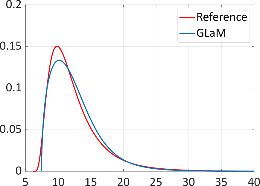
(a) PDF for $\bm{x}=(5\pi/3,\pi/2,0.6)$

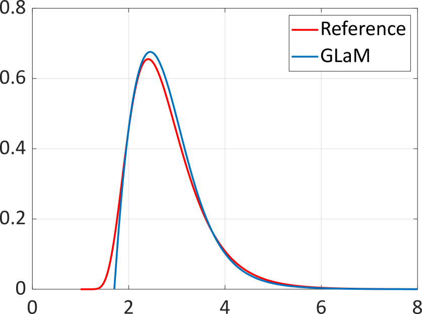
(b) PDF for $\bm{x}=(\pi/3,\pi,0.4)$

Figure 1: Toy example – Emulated response PDFs, $N=1{,}000$

.

Figure 1(b) compares the PDFs predicted by a GLaM built on an experimental design of $N=1{,}000$ with the reference response PDFs of the simulator. The results show that the developed algorithm correctly identifies the shape of the underlying shifted lognormal distribution. Moreover, the PDF supports and tails are also accurately approximated.

We consider the differential entropy $h(\bm{x})$ [12] as the QoI in this example. Because the analytical response distribution and entropy are known, we investigate the convergence of GLaM in terms of the conditional quantile function estimation Equation 29 and the entropy estimation Equation 28. The size of experimental design varies among $N\in\left\{250;500;1{,}000;2{,}000;4{,}000\right\}$. Note that the entropy of a GLD does not have a closed form. Therefore, we use $10^{4}$ Monte Carlo samples to estimate this quantity of a GLaM for each $\bm{x}$ in the test set.

In addition, we consider another model where we approximate the response distribution with a normal distribution. The mean and variance (as functions of $\bm{x}$) for such an approximation are chosen as the true mean and variance of the original. In other words, this model represents the “oracle” of Gaussian-type mean-variance models.

The results are summarized in Figure 2. The proposed method exhibits a clear convergence with respect to $N$ for both $Q(u;\bm{x})$ and $h(\bm{x})$ estimations. We observe in Figure 2(a) that the decay of $\varepsilon_{Q}$ has two regimes separated by $N=1{,}000$. For a small $N$, the error coming from the use of finite samples dominates the estimate accuracy. When we consider a large data set, the error mainly comes from the model mispecification, because the stochastic simulator cannot be exactly represented by a GLaM. This phenomenon is not significant for the entropy estimation, which demonstrates a relatively consistent decay.

The accuracy of the oracle normal approximation is reported with red dash lines in Figure 2. The error shown is only due to model misspecifications (because the true response distribution is not Gaussian) since we use the underlying true mean and variance. For both measures, the medians of the errors of GLaMs built on $N=250$ model runs are smaller than those of the normal approximation. For $N\geq 1{,}000$, the GLaM clearly outperforms the oracle of Gaussian-type mean-variance models. This example illustrates the limits of such Gaussian-type models in practice.

Finally, the errors of GLaMs are below $0.05$ for $N\geq 1{,}000$ indicating that the surrogate is able to explain over 95% of the variance of the target functions.

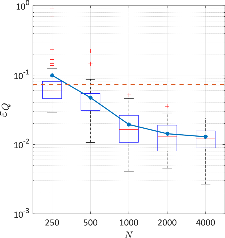
(a) Conditional quantile function estimation

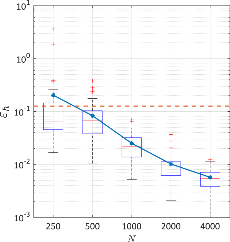
(b) Entropy estimation

Figure 2: Toy example – Convergence study. The blue lines denote the errors averaged over 50 repetitions of the full analysis. The red dash lines are the corresponding errors of the model assuming that the response distribution is normal with the true mean and variance

For sensitivity analysis, we focus on the classical first-order and the entropy-based total Sobol’ indices. Figure 3 and Figure 4 show the convergence of GLaMs for estimating these quantities of each input variable. The reference values are derived from Equation 30. As shown by the two figures, this toy example is designed to have $X_{2}$ as the most important variable according to the classical first-order Sobol’ indices, which also indicates that $X_{2}$ contributes the most to the variance of the mean function $m(\bm{X})$. In contrast, it has zero effect to the entropy. In comparison, $X_{1}$ is the dominant variable for the variation of the entropy $h(\bm{X})$. Because $X_{3}$ mainly controls the shape of the response distribution (especially the right tail), it has a minor first-order effect to the mean function, which leads to a very small value of $S_{3}$. In contrast, the entropy depends on the distribution shape, and thus $S^{h}_{T_{3}}$ is not negligible. The results reveal that GLaMs capture this characteristic and yield accurate estimates for both classical Sobol’ indices and entropy-based Sobol’ indices.

Similar to Figure 2, we also reported the sensitivity indices calculated by using Gaussian approximations with the true mean and variance. Because the classical first-order indices depend only on the mean and variance functions, the oracle Gaussian model gives the exact values. Therefore, we showed only the results for the entropy-based Sobol’ indices in Figure 4. It is clear that the Gaussian approximation with the true mean and variance demonstrates a significant bias. In contrast, GLaMs show nearly no bias and approximate much more accurately the reference values.

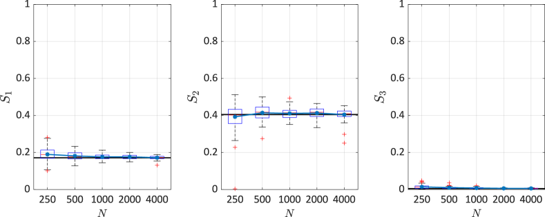
Figure 3: Estimation of the classical first-order Sobol’ indices. The black lines are the reference values, and the blue lines denote the average values of 50 repetitions of the full analysis.

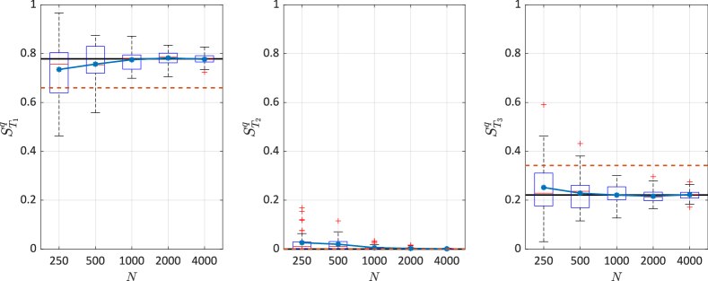
Figure 4: Estimation of the entropy-based total Sobol’ indices. The black lines are the reference values, and the blue lines denote the average values of 50 repetitions of the full analysis. The red dash lines correspond to the indices calculated from the normal approximation using the true mean and variance

4.2 Heston model

In this example, we perform the global sensitivity analysis for a Heston model used in mathematical finance [37]. The Heston model describes the evolution of a stock price $Y_{t}$. It is an extension of the geometric Brownian motion by modeling the volatility as a stochastic process $v_{t}$, instead of considering it as constant. Hence, the Heston model is a stochastic volatility model and consists of two coupled stochastic differential equations:

$$\begin{split}\mathrm{d}Y_{t}&=\mu Y_{t}\mathrm{d}t+\sqrt{v_{t}}Y_{t}\mathrm{d}W^{1}_{t},\\ \mathrm{d}v_{t}&=\kappa(\theta-v_{t})\mathrm{d}t+\sigma\sqrt{v_{t}}\mathrm{d}W^{2}_{t},\end{split}$$ (31)

with

$${\mathbb{E}}\left[\mathrm{d}W^{1}_{t}\,\mathrm{d}W^{2}_{t}\right]=\rho\mathrm{d}t,$$ (32)

where $W^{1}_{t}$ and $W^{2}_{t}$ are two Wiener processes with correlation coefficient $\rho$, which introduce the intrinsic randomness of the stochastic model. The model parameters $\bm{x}=(\mu,\kappa,\theta,\sigma,\rho,v_{0})$ are summarized in Table 1. The range of the last five input variables are selected based on the parameters calibrated from real data (S&P 500 and Eurostoxx 50) [38]. The range of the first variable $\mu$ is set to $[0,0.1]$ to take the uncertainty of the expected return rate into account. Without loss of generality, we set $Y_{0}=1$.

Table 1: Parameters of the Heston model

Variable	Description	Distribution
$\mu$	Expected return rate	${\mathcal{U}}(0,0.1)$
$\kappa$	Mean reversion speed of the volatility	${\mathcal{U}}(0.3,2)$
$\theta$	Long term mean of the volatility	${\mathcal{U}}(0.02,0.07)$
$\sigma$	Volatility of the volatility	${\mathcal{U}}(0.2,0.4)$
$\rho$	Correlation coefficient between $\mathrm{d}W^{1}_{t}$ and $\mathrm{d}W^{2}_{t}$	${\mathcal{U}}(-1,-0.5)$
$v_{0}$	Volatility at time 0	${\mathcal{U}}(0.02,0.07)$

In this example, we are interested in the stock price after one year, i.e., $Y_{t}(\bm{x})$ with $t=1$. A closed form solution to Equation 31 is generally not available. To get samples of $Y_{1}(\bm{x})$, we simulate the entire time evolution of $Y_{t}$ and $v_{t}$ for a given $\bm{x}$ using Euler integration scheme with $\Delta t=0.001$ over the time interval $[0,1]$. Note that when simulating the bivariate process $(Y_{t},v_{t})$, a problem may happen: since $v_{t}$ follows a Cox–Ingersoll–Ross process [38], the simulation scheme can generate negative values for $v_{t}$. To overcome the problem, we apply the full truncation scheme, which replaces the update of $v_{t}$ by $\max\left(v_{t},0\right)$ [38].

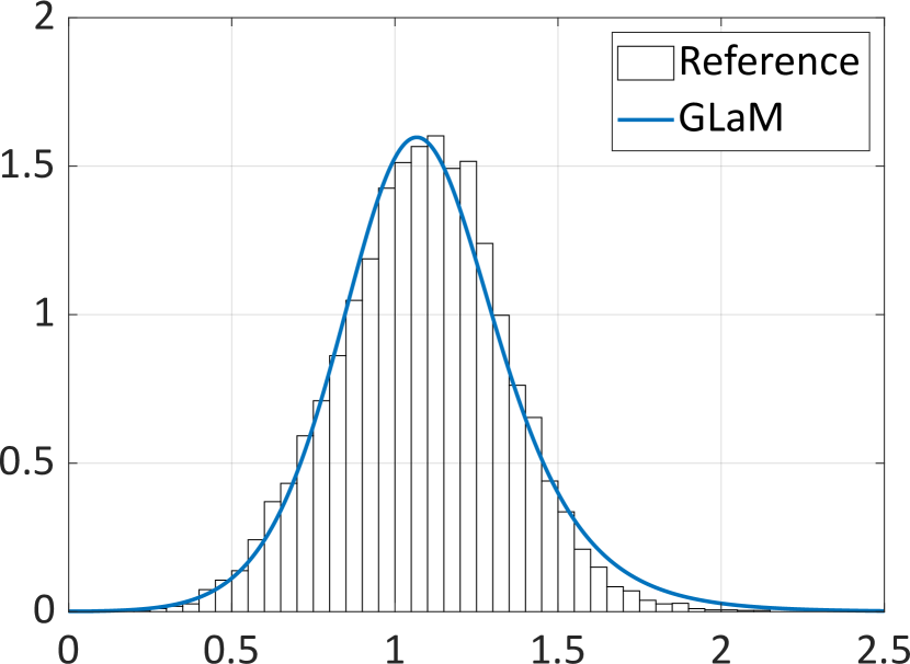
(a) PDF for $\bm{x}=(0.08,1.6,0.06,0.35,-0.6,0.06)$

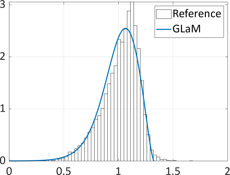
(b) PDF for $\bm{x}=(0.02,0.5,0.03,0.25,-0.8,0.03)$

Figure 5: Heston model – Emulated response PDFs, $N=2{,}000$

Figure 5 shows two response PDFs predicted by a surrogate built upon $N=2{,}000$ model runs. The reference histograms are obtained from $10^{4}$ repeated model runs with the same input parameters. We observe that the variance of the response distribution is not constant, e.g., 0.065 and 0.027 for the two illustrated PDFs. Moreover, the PDF shape varies: it changes from symmetric to left-skewed distributions depending on the model parameters. This would be difficult to approximate with a simple distribution family such as normal or lognormal. In contrast, GLaMs are able to accurately capture this shape variation, because of the flexibility of generalized lambda distributions.

Even though a closed form distribution of $Y_{1}(\bm{x})$ does not exist, the mean function $m(\bm{x})={\mathbb{E}}\left[Y_{1}(\bm{x})\right]$ can be derived analytically:

$$m(\bm{x})=\exp(x_{1})=\exp(\mu).$$ (33)

As a result, we use $\varepsilon_{m}$ defined in Equation 29 with ${\rm QoI}(\bm{x})=m(\bm{x})$ to assess the convergence of the surrogate. In addition, we also consider the expected payoff of an European call option. The payoff $C(\bm{x})$ and the expected payoff $m_{C}(\bm{x})$ of an European call option are defined by

$$\begin{split}C(\bm{x})&=\max\left\{0,Y_{1}(\bm{x})-K\right\},\\ m_{C}(\bm{x})&={\mathbb{E}}\left[C(\bm{x})\right],\end{split}$$ (34)

where $K$ is the strike price and set to $1$ in the following analysis. In finance, $m_{C}$ not only is important for making investment decisions but also has a very similar form to the option price [39]. For the Heston model, numerical methods based on the Fourier transform have been developed to calculate the expected payoff without the need for Monte Carlo simulations [37]. For the GLaM surrogate, this quantity can also be calculated numerically (see Section 6.1). As a second performance index, we compute the associated error denoted by $\varepsilon_{C}$ (Equation 29) for the convergence study.

Figure 6 shows box plots of the errors $\varepsilon_{m}$ and $\varepsilon_{c}$ for $N\in\{500;1{,}000;\allowbreak 2{,}000;\allowbreak 4{,}000;\allowbreak 8{,}000;16{,}000\}$. Both $\varepsilon_{m}$ and $\varepsilon_{c}$ are relatively large for $N\leq 2{,}000$. This is mainly due to the fact that the variability of the model response is dominated by the intrinsic randomness: the model parameters $\bm{X}$ altogether are only able to explain about 2% of the variance of the output (i.e., $S_{\left\{1,\ldots,6\right\}}=0.02$). In other words, the stochastic simulator has a very small signal-to-noise ratio ${\rm SNR}=0.02/(1-0.02)\approx 0.02$. Since GLDs are flexible, a few data scattered in a moderately high dimensional space may not provide enough information of the response distribution variation. We observe that for $N\leq 1{,}000$, the selection procedure proposed in Algorithm 1 can choose $\lambda^{\operatorname*{PC}}_{1}(\bm{x})$ and $\lambda^{\operatorname*{PC}}_{2}(\bm{x})$ being only constant. Such a model is too simple and thus fails to capture the variations of the scalar quantities. Consequently, it is necessary to have enough data to achieve an accurate estimate: when increasing the size of $N$ of the LHS design, we observe a clear decay of the errors.

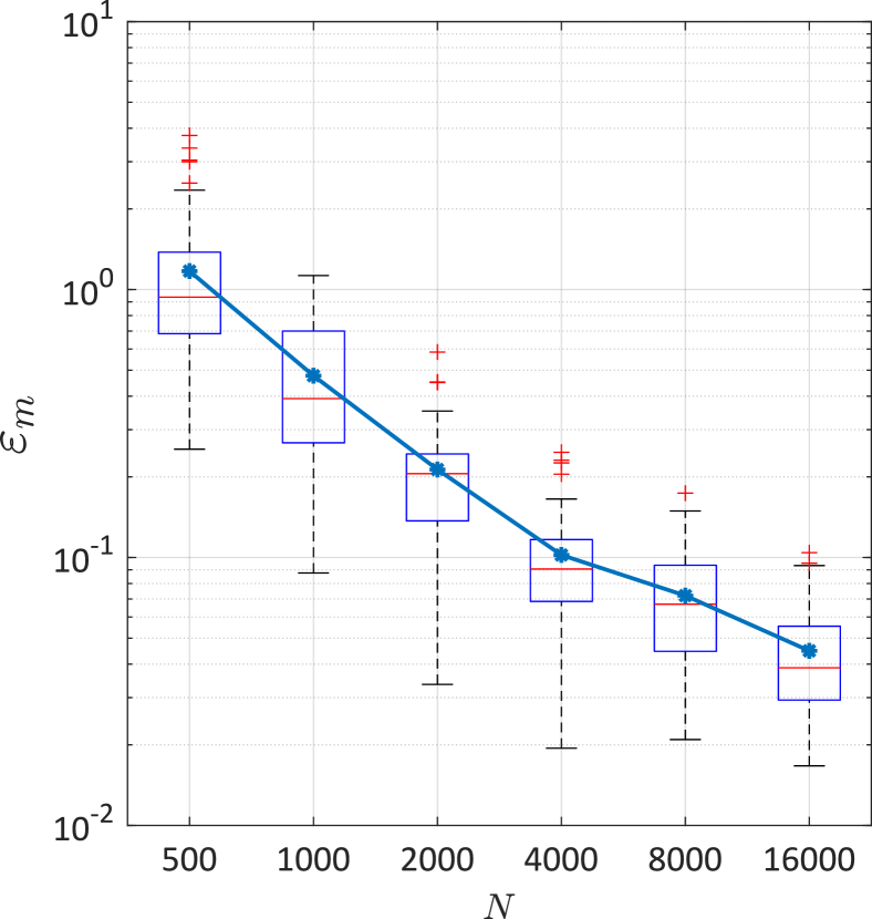
(a) Mean estimation

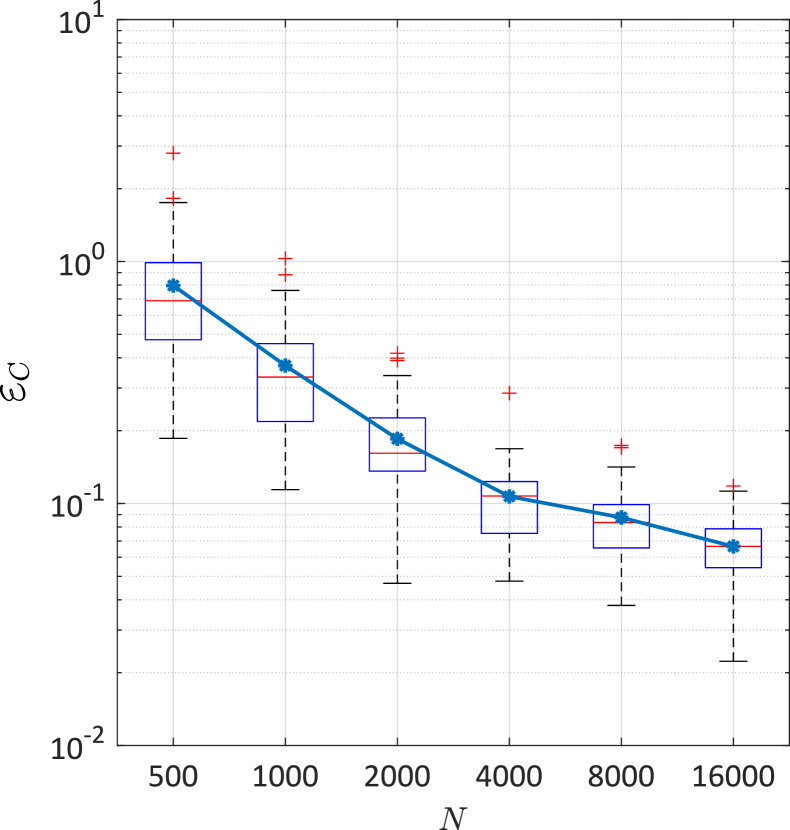
(b) Expected payoff estimation

Figure 6: Heston model – Convergence study. The blue lines denote the errors averaged over 50 repetitions of the full analysis.

We now study the convergence for the Sobol’ indices estimations. According to Equation 33, the mean function depends only on the first input variable $X_{1}$, which contributes little (2%) to the total variance of $Y_{1}(\bm{X})$. This implies that the classical Sobol’ indices are not informative (they are either 0 or very close to 0). However, we cannot ignore the variability of the input variables because the response distribution demonstrates a clear dependence on the input parameters, as shown in Figure 5. Therefore, we focus on the accuracy of the expected-payoff-based total Sobol’ indices, denoted by $S^{C}_{T_{{\bm{\mathsf{u}}}}}$.

As a second quantity of interest, we also calculate the total Sobol’ indices associated to the $95\%$-superquantile, referred to as $S^{\rm sq}_{T_{{\bm{\mathsf{u}}}}}$. Superquantiles are known as the conditional value-at-risk, which is an important risk measure in finance [40]. The $\alpha$-superquantile of a random variable $Y$ is defined by

$${\rm sq}_{\alpha}={\mathbb{E}}\left[Y\mid Y\geq q_{\alpha}\right],$$ (35)

where $q_{\alpha}$ is the $\alpha$-quantile of $Y$. This quantity corresponds to the conditional expectation of $Y$ being larger than its $\alpha$-quantile. For the Heston model, this quantity does not have an analytical closed form, whereas ${\rm sq}_{\alpha}$ of a GLD can be derived analytically (see Section 6.1).

We use $10^{5}$ Monte Carlo samples to evaluate (numerically) the function $m_{C}(\bm{x})$ to obtain a reference value for each $S^{C}_{T_{{\bm{\mathsf{u}}}}}$. To calculate the Sobol’ indices associated to the 95%-superquantile ${\rm sq}_{95}(\bm{X})$, it is necessary to evaluate the function ${\rm sq}_{95}(\bm{x})$. Because it cannot be analytically derived for the Heston model, we use $10^{4}$ replications to calculate the sample 95%-superquantile $\hat{{\rm sq}}_{95}(\bm{x})$ as an estimate for ${\rm sq}_{95}(\bm{x})$. Then, we treat it as a deterministic function and use $10^{4}$ samples to estimate each Sobol’ index. This indicates that a total number of $7\times 10^{8}$ model runs are performed to obtain the six reference 95%-superquantile-based total Sobol’ indices. Because only $10^{4}$ samples are used to estimate each $S^{\rm sq}_{T_{{\bm{\mathsf{u}}}}}$, we use bootstraps [41] to calculate the 95% confidence interval to account for the uncertainty of the Monte Carlo simulation.

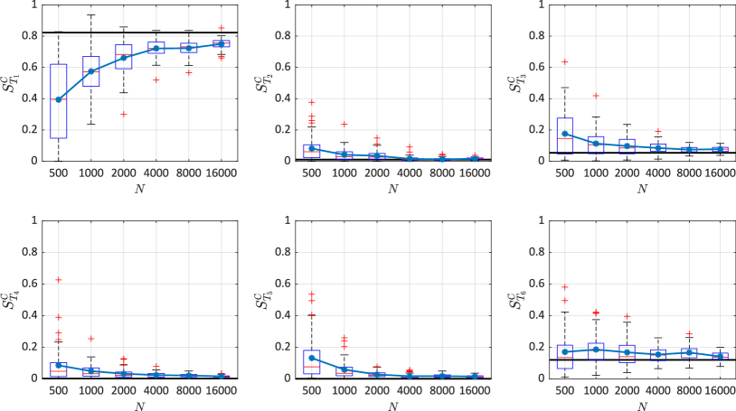
Figure 7: Estimation of the expected-payoff-based total Sobol’ indices. The black lines are the reference values, and the blue lines denote the average values of 50 repetitions.

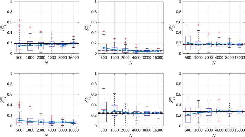
Figure 8: Estimation of the 95%-superquantile-based total Sobol’ indices. The blue lines denote the average value of 50 repetitions of the full analysis. The black lines are the reference values, and the dashed lines correspond to the 95% confidence intervals.

Figures 7 and 8 confirm and quantify the convergence of GLaMs to estimate $S^{C}_{T_{{\bm{\mathsf{u}}}}}$ and $S^{\rm sq}_{T_{{\bm{\mathsf{u}}}}}$. For the expected payoff $m_{C}(\bm{x})$, the first variable $\mu$ is the most important. The estimation of its total effect converges from below the reference value, and we observe a bias in the estimate. Nevertheless, with $N$ large enough ($\geq 4{,}000$), the GLaM can always correctly identify its importance (the bias is 0.072 for $\geq 8{,}000$ and 0.055 for $\geq 16{,}000$), and each classical first-order Sobol’ index of the other five variables converge to the reference line. The 95%-superquantile suggests a different ranking: $\mu$, $\theta$, $\rho$ and $v_{0}$ (corresponding to the first, third, fifth and sixth input variable, respectively) have similar total effects, which are superior to those of $\kappa$ and $\sigma$ (i.e., the second and fourth input variables). In addition, none of the input variables has nearly 0 total effect. The GLaM surrogate model accurately reproduces the phenomena. Moreover, the estimates generally vary around the reference values, and larger $N$ results in narrower spread of the box plots.

As a conclusion, GLaM surrogates allow us to represent accurately the QoI of the Heston model and carry out a detailed sensitivity analysis at the cost of $\mathcal{O}(10^{4})$ runs of the stochastic simulator. Note that in this example the leave-one-out errors of the polynomial chaos expansions built on the GLaM surrogates are of the order of $o(10^{-4})$, which justifies the use of PCE-based Sobol’ indices.

4.3 Stochastic SIR model

In this example, we apply the proposed method to a stochastic Susceptible-Infected-Recovered (SIR) model in epidemiology [3]. This model simulates the spread of an infectious disease, which can help conduct appropriate epidemiological intervention to minimize the social and ethical impacts during the outbreak.

In a SIR model, a population of size $P_{t}$ at time $t$ can be partitioned into three groups: susceptible, infected and recovered during the outbreak of an epidemic. Susceptible individuals are those who can get infected by contacting an infectious person. Infected individuals are suffering from the disease and are contagious. They can recover (therefore classified as recovered) and become immune to future infections. The number of individuals within each group is denoted by $E_{t}$, $I_{t}$ and $R_{t}$, respectively. Without differentiating individuals, these three quantities characterize the configuration of the population at a given time $t$. Hence, their evolutions represent the spread of the epidemic. In this study, we consider a fixed population without newborns and deaths, i.e., the total population size is constant, $P_{t}=P$. As a result, $E_{t}$, $I_{t}$ and $R_{t}$ satisfy the constraint $E_{t}+I_{t}+R_{t}=P$, and thus only the time evolution of $E_{t}$ and $I_{t}$ is necessary to represent the disease evolution.

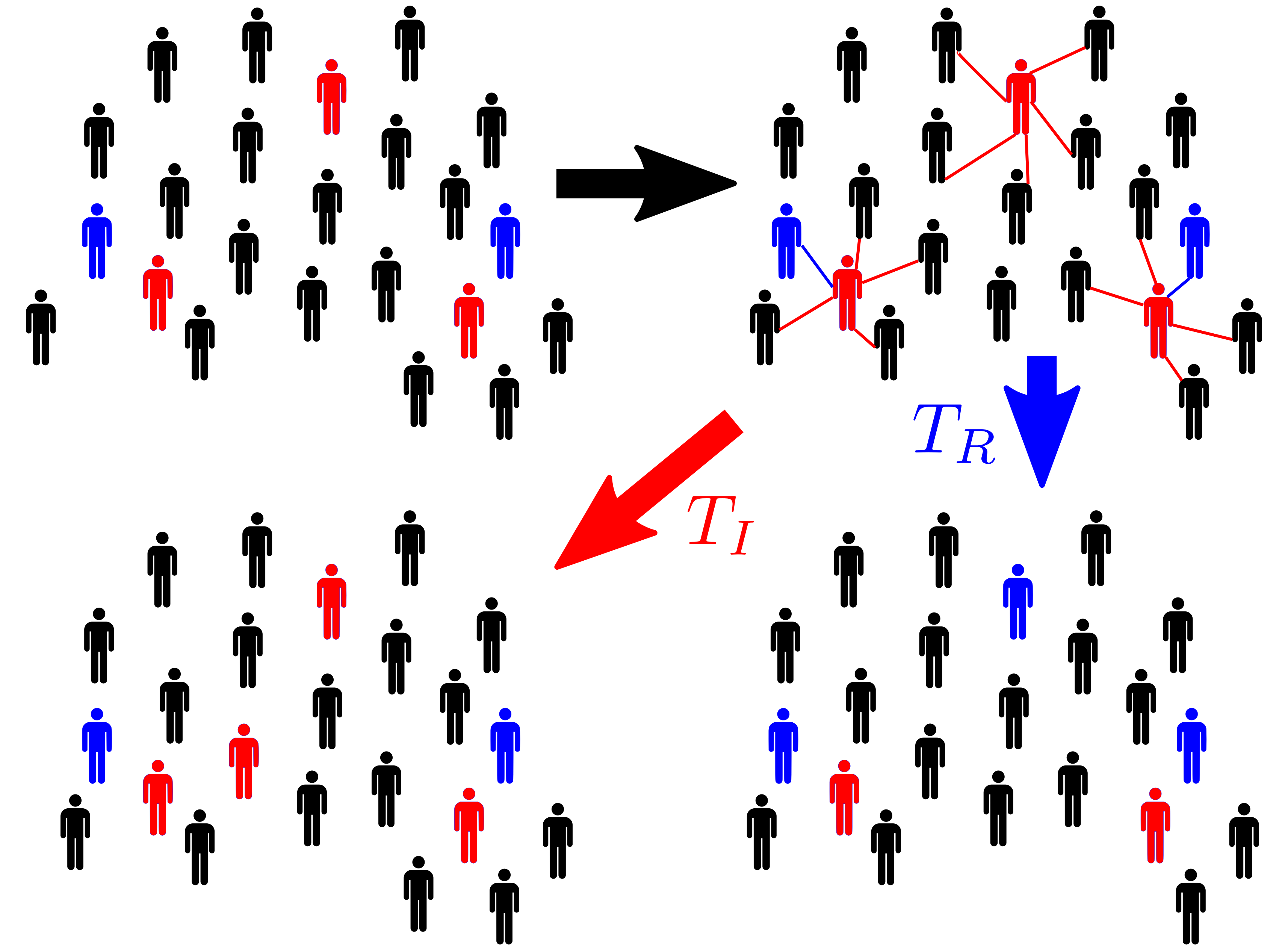
Figure 9: Dynamics of the stochastic SIR model: black icons denote susceptible individuals, red icons represent infected individuals, and blue icons are those recovered.

Without going into detailed assumptions of the model, we illustrate the system dynamics in Figure 9, where the black icons represent susceptible individuals, the red icons indicate infected persons, and the blue icons are those recovered. Suppose that at time $t$ the population has the configuration $(E_{t},I_{t})$ (top left figure of Figure 9). Infected individuals can meet susceptible individuals, or they may receive essential treatments and recover from the disease. Hence, the next configuration has two possibilities: (1) $C_{I}$, where one susceptible individual is infected; (2) $C_{R}$, where one infected person recovers. The population state evolving either to $C_{I}$ or $C_{R}$ depends on two random variables, $T_{I}$ and $T_{R}$, which denote the respective time to move to the associated candidate configuration. Both random variables follow an exponential distribution, yet with different parameters:

$$T_{I} \sim{\rm Exp}(\lambda_{I}),\quad\lambda_{I}=\beta\frac{E_{t}I_{t}}{P},$$ (36)

$$T_{R} \sim{\rm Exp}(\lambda_{R}),\quad\lambda_{R}=\gamma I_{t},$$ (37)

where $\beta$ indicates the contact rate of an infected individual, and $\gamma$ is the recovery rate. If $T_{I}>T_{R}$, $C_{I}$ becomes the next configuration at $t+T_{I}$ with $S_{t+T_{I}}=E_{t}-1$ and $I_{t+T_{I}}=I_{t}+1$, and vice versa. This update step iterates until time $T$ when $I_{T}=0$. Because the population size is finite and the recovered individuals will not get infected again, the total number of updates is finite ($\leq P$). This number is not a constant due to the updating process, indicating that the amount of latent variables of this simulator is also random. Note that the evolution procedure described here corresponds to the Gillespie algorithm [42].

In this case study, we set $P=2{,}000$. $\bm{x}=(E_{0},I_{0},\beta,\gamma)$ is the vector of input parameters. To account for different scenarios, the input variables $\bm{X}$ are modeled as $X_{1}\sim{\mathcal{U}}(1{,}600\,,\,1{,}800)$, $X_{2}\sim{\mathcal{U}}(20,200)$ and $X_{3},X_{4}\sim{\mathcal{U}}(0.5,0.7)$. The uncertainty in the first two variables can be interpreted as lack of knowledge of the initial condition. While the last two variables are affected by possible interventions, such as social distancing measures that can reduce the contact rate $\beta$ and increasing medical resources that improves the recovery rate $\gamma$. We are interested in the total number of newly infected individuals during the outbreak, i.e., $E_{T}-E_{0}$. The signal-to-noise ratio of this stochastic model is estimated to be ${\rm SNR}\approx 6.7$, which is relatively large.

Figure 10 shows the response PDF estimation of the surrogate model built on an experimental design of $N=1{,}000$. The reference histograms are calculated from $10^{4}$ repeated model runs with the same input values. We observe that the response distribution changes from right-skewed to left-skewed distributions (so we can also find symmetric distributions in between), which is correctly represented by the surrogate. In addition, GLaMs also accurately approximate the bulk and the support of the response PDF.

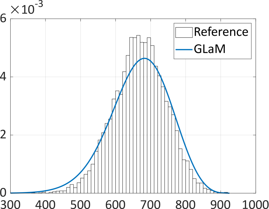
(a) PDF for $\bm{x}=(1750,150,0.55,0.65)$

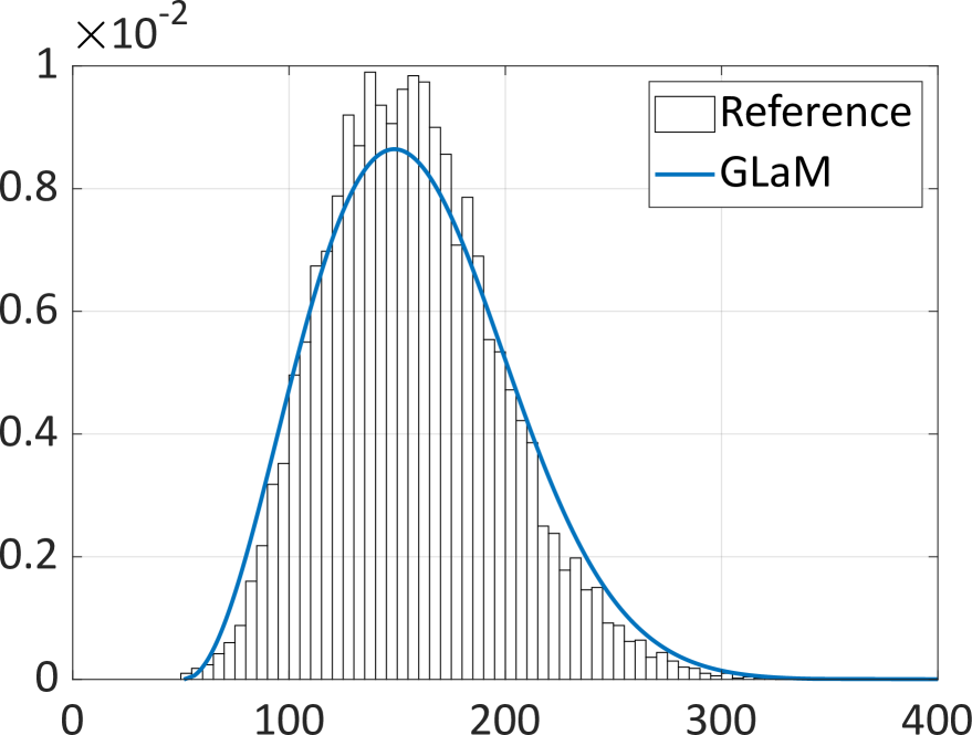
(b) PDF for $\bm{x}=(1650,80,0.65,0.55)$

Figure 10: Stochastic SIR model – Emulated response PDFs, $N=1{,}000$

In this example, we investigate the convergence of GLaMs for estimating the classical first-order Sobol’ indices and the standard-deviation-based total Sobol’ indices, denoted by $S^{\sigma}_{T_{{\bm{\mathsf{u}}}}}$. To calculate the reference values, we use $10^{5}$ Monte Carlo samples for each classical Sobol’ index. Regarding the standard-deviation-based Sobol’ indices, we calculate the sample standard deviation $\hat{\sigma}(\bm{x})$ based on $10^{4}$ replications. Then, we apply Monte Carlo simulations with $10^{4}$ samples to estimate the associated Sobol’ indices. The total cost to get reference values is thus equal to $5\times 10^{8}$. As in the previous example, we use bootstraps to calculate the 95% confidence intervals.

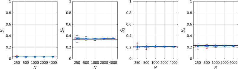
Figure 11: Estimation of the classical first-order Sobol’ indices. The black lines are the reference values, and the blue lines denote the average values of 50 repetitions of the full analysis.

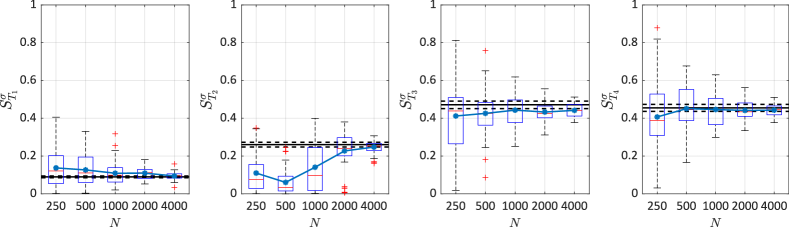
Figure 12: Estimation of the standard-deviation-based total Sobol’ indices. The blue lines denote the average values of 50 repetitions of the full analysis. The black lines are the reference values, and the dashed lines correspond to the 95% confidence intervals.

Figures 11 and 12 show the results of the convergence study. In terms of the classical Sobol’ indices, the GLaM yields accurate estimates even when $N=250$: the box plots scatter around the reference values with a small variability. Among the four input variables, the second one $I_{0}$ that corresponds to the number of infected individuals at time 0 is the most important. It is followed by the contact rate and the recovery rate, which show similar first-order effect. As a result, performing medical test to better determine $I_{0}$ would be the most effective way to reduce the variance of the output. In contrast, Figure 12 suggests that controlling the contact rate and recovery rate would be the best measure to reduce the variation of $\sigma(\bm{X})$. For estimating the associated Sobol’ indices, the GLaM converges within the 95% confidence intervals of the Monte Carlo estimates, and the spread of the box plots decreases significantly with $N$ increasing.

Finally, we remark that when higher-order Sobol’ indices are of interest, Monte Carlo simulations require additional runs of the original model. For example, $4\times 10^{8}$ more model evaluations should be performed to obtain the reference values for the standard-deviation-based second-order Sobol’ indices. This results in a large amount of total model runs, which become impracticable even with cheap models. In contrast, GLaM surrogates can be used without additional cost: the PCE-based method presented in Section 3.5.3 provides analytical higher-order indices by post-processing the PC coefficients. In this example, the leave-one-out errors of PCE built on the GLaM surrogates are of the order $\mathcal{O}(10^{-3})$, which justifies the use of PCE estimates. Based on the surrogate model, we observe that the largest standard-deviation-based second-order Sobol’ indices, which translate parameters interactions, are $I_{0}$ and $\beta$, $I_{0}$ and $\gamma$. Both have a value 0.09, while the other second-order interactions are very small. As illustrated in Figure 12, $I_{0}$ has a total effect $S^{\sigma}_{T_{2}}=0.26$. Moreover, it has a relatively small first-order effect $S^{\sigma}_{2}=0.05$. This implies that $I_{0}$ mainly affects the variance of $\sigma(\bm{X})$ through its interactions with $\beta$ and $\gamma$.

5 Conclusions

In this paper, we discuss the nature and focus of three extensions of Sobol’ indices to stochastic simulators: classical Sobol’ indices, QoI-based Sobol’ indices and trajectory-based Sobol’ indices. The first two types are of interest because of their versatility and applicability to a broad class of problems. We propose to use the generalized lambda model as a stochastic emulator to estimate the considered indices. This surrogate model aims at emulating the entire response distribution, instead of focusing only on some scalar statistical quantities, e.g., mean and variance. More precisely, it relies on using the four-parameter generalized lambda distribution to approximate the response distribution. The associated distribution parameters as functions of the input are represented by polynomial chaos expansions. Such a surrogate can be constructed without the need for replications, and thus it is not restricted to a special data structure.

Because of the special formulation of GLaM, the considered sensitivity indices can be estimated by directly working with deterministic functions. This allows applying the methods developed for deterministic simulators, namely estimators based on Monte Carlo simulations and on polynomial chaos expansions. In this paper, we suggest the latter to post-process the surrogate model to achieve high computational efficiency.

The performance of the proposed method for estimating various Sobol’ indices is illustrated on three examples with different signal-to-noise ratios. The toy example is designed to have a strong heteroskedastic effect. It shows the general convergent behavior of GLaMs for approximating the conditional quantile functions and estimating the entropy of the response distributions. The second example is a Heston model from mathematical Finance. This case study has a very small signal-to-noise ratio and demonstrates a shape variation of the response PDF. The surrogate generally yields accurate estimate of the Sobol’ indices associated to the expected payoff and the 95%-superquantile. The last example is a stochastic SIR model in epidemiology, in which GLaMs exhibit robust estimates of the classical Sobol’ indices and the standard-deviation-based Sobol’ indices. All three examples have a different ranking of the input variables depending on the type of Sobol’ indices, which is correctly captured by GLaMs when comparing to reference values obtained by extremely costly Monte Carlo simulations. Fairly accurate results are obtained at a cost of $\mathcal{O}\left(10^{4}\right)$ runs of the simulator compared to reference values based on $\mathcal{O}\left(10^{8}\right)$ runs by a brute force approach.

In future work, we plan to develop algorithms to improve GLaMs for small data sets. Besides, we will investigate GLaMs for estimating distribution-based sensitivity indices [43, 44]. The estimation of these indices usually requires a large number of model runs to infer the conditional PDF, which can be easily obtained from GLaMs. In addition, appropriate contrast measures between distributions, such as the Wasserstein metric, can be developed for sensitivity analysis in the context of stochastic simulators. Finally, developing sensitivity indices for stochastic simulators with dependent input variables will allow engineers to tackle a broader group of problems.

6 Appendix

6.1 Some properties of GLDs

The mean and variance of a GLD can be calculated by

$$m =\lambda_{1}-\frac{1}{\lambda_{2}}\left(\frac{1}{\lambda_{3}+1}-\frac{1}{\lambda_{4}(\bm{x})+1}\right),$$ (38)

$$v =\frac{(d_{2}-d_{1}^{2})}{\lambda_{2}^{2}},$$ (39)

where $\left\{d_{k}:k=1,2\right\}$ are defined by

$$\begin{split}d_{1}&=\frac{1}{\lambda_{3}}\operatorname{B}(\lambda_{3}+1,1)-\frac{1}{\lambda_{4}}\operatorname{B}(1,\lambda_{4}+1),\\ d_{2}&=\frac{1}{\lambda^{2}_{3}}\operatorname{B}(2\lambda_{3}+1,1)-\frac{2}{\lambda_{3}\lambda_{4}}\operatorname{B}(\lambda_{3}+1,\lambda_{4}+1)+\frac{1}{\lambda^{2}_{4}}\operatorname{B}(1,2\lambda_{4}+1),\end{split}$$ (40)

with $\operatorname{B}$ denoting the beta function.

The expected payoff defined in Equation 41 of a GLD with the strike price $K$ is given by

$$\begin{split}m_{C}&\stackrel{{\scriptstyle\text{def}}}{{=}}{\mathbb{E}}\left[\max\left\{Y-K,0\right\}\right]\\ &=\left(\lambda_{1}-\frac{1}{\lambda_{2}\lambda_{3}}+\frac{1}{\lambda_{2}\lambda_{4}}-K\right)\,(1-u_{K})+\frac{1}{\lambda_{2}}\,\left(\frac{1-u_{K}^{\lambda_{3}+1}}{\lambda_{3}\,\left(\lambda_{3}+1\right)}-\frac{(1-u_{K})^{\lambda_{4}+1}}{\lambda_{4}\,\left(\lambda_{4}+1\right)}\right).\end{split}$$ (41)

where $u_{K}$ is the solution of the nonlinear equation:

$$Q(u_{K};\bm{\lambda})=K.$$ (42)

The $\alpha$-superquantile ${\rm sq}_{\alpha}$ defined in Equation 35 of a GLD has a closed-form:

$$\begin{split}{\rm sq}_{\alpha}&\stackrel{{\scriptstyle\text{def}}}{{=}}{\mathbb{E}}\left[Y\mid Y>q_{\alpha}\right]\\ &=\lambda_{1}-\frac{1}{\lambda_{2}\lambda_{3}}+\frac{1}{\lambda_{2}\lambda_{4}}+\frac{1}{(1-\alpha)\lambda_{2}}\,\left(\frac{1-\alpha^{\lambda_{3}+1}}{\lambda_{3}\,\left(\lambda_{3}+1\right)}-\frac{\alpha^{\lambda_{4}+1}}{\lambda_{4}\,\left(\lambda_{4}+1\right)}\right).\end{split}$$ (43)

References

- [1] S. Azzi, Y Huang, B. Sudret, and J. Wiart. Surrogate modeling of stochastic functions – application to computational electromagnetic dosimetry. Int. J. Uncertainty Quantification, 9(4):351–363, 2019.
- [2] A. J. McNeil, R. Frey, and P. Embrechts. Quantitative Risk Management: Concepts, Techniques, and Tools. Princeton Series in Finance. Princeton University Press, Princeton, New Jersey, 2005.
- [3] T. Britton. Stochastic epidemic models: a survey. Math. Biosci., 225:24–35, 2010.
- [4] A. Saltelli, K. Chan, and E. M. Scott, editors. Sensitivity analysis. J. Wiley & Sons, 2000.
- [5] E. de Rocquigny, N. Devictor, and S. Tatantola. Uncertainty in Industrial Practice: A guide to Quantitative Uncertainty Management. J. Wiley & Sons, New York, 2008.
- [6] J.C. Helton, J.D. Johnson, C.J. Sallaberry, and C.B. Storlie. Survey of sampling-based methods for uncertainty and sensitivity analysis. Reliab. Eng. Sys. Safety, 91(10–11):1175–1209, 2006.
- [7] E. Borgonovo. Sensitivity analysis – An Introduction for the Management Scientist. Springer, 2017.
- [8] I. M. Sobol’. Sensitivity estimates for nonlinear mathematical models. Math. Modeling & Comp. Exp., 1:407–414, 1993.
- [9] B. Iooss and M. Ribatet. Global sensitivity analysis of computer models with functional inputs. Reliab. Eng. Sys. Safety, 94:1194–1204, 2009.
- [10] J.L. Hart, A. Alexanderian, and P.A. Gremaud. Efficient computation of Sobol’ indices for stochastic models. SIAM J. Sci. Comput., 39:1514–1530, 2016.
- [11] M. N. Jimenez, O. P. Le Maître, and O. M. Knio. Nonintrusive polynomial chaos expansions for sensitivity analysis in stochastic differential equations. SIAM J. Uncer. Quant., 5:212–239, 2017.
- [12] S. Azzi, B. Sudret, and J. Wiart. Sensitivity analysis for stochastic simulators using differential entropy. Int. J. Uncertainty Quantification, 10:25–33, 2020.
- [13] M. Dacidian and R. J. Carroll. Variance function estimation. J. Amer. Stat. Assoc., 400:1079–1091, 1987.
- [14] A. Marrel, B. Iooss, S. Da Veiga, and M. Ribatet. Global sensitivity analysis of stochastic computer models with joint metamodels. Stat. Comput., 22:833–847, 2012.
- [15] M. Binois, R. Gramacy, and M. Ludkovski. Practical heteroskedastic Gaussian process modeling for large simulation experiments. J. Comput. Graph. Stat., 27:808–821, 2018.
- [16] X. Zhu and B. Sudret. Replication-based emulation of the response distribution of stochastic simulators using generalized lambda distributions. Int. J. Uncertainty Quantification, 10(3):249–275, 2020.
- [17] X. Zhu and B. Sudret. Emulation of stochastic simulators using generalized lambda models. Submitted to SIAM/ASA J. Unc. Quant., 2021. (ArXiv: 2007.00996).
- [18] Z. A. Karian and E. J. Dudewicz. Fitting Statistical Distributions: The Generalized Lambda Distribution and Generalized Bootstrap Methods. Chapman and Hall/CRC, 2000.
- [19] R. Ghanem and P. Spanos. Stochastic Finite Elements: A Spectral Approach. Courier Dover Publications, Mineola, 2nd edition, 2003.
- [20] T. Homma and A. Saltelli. Importance measures in global sensitivity analysis of non linear models. Reliab. Eng. Sys. Safety, 52:1–17, 1996.
- [21] T. Browne, B. Iooss, L. Le Gratiet, J. Lonchampt, and E. Rémy. Stochastic simulators based optimization by Gaussian process metamodels – application to maintenance investments planning issues. Quality Reliab. Eng. Int., 32(6):2067–2080, 2016.
- [22] M. Freimer, G. Kollia, G. S. Mudholkar, and C. T. Lin. A study of the generalized Tukey lambda family. Comm. Stat. Theor. Meth., 17:3547–3567, 1988.
- [23] O. G. Ernst, A. Mugler, H. J. Starkloff, and E. Ullmann. On the convergence of generalized polynomial chaos expansions. ESAIM: Math. Model. and Num. Anal., 46:317–339, 2012.
- [24] D. Xiu and G. E. Karniadakis. The Wiener-Askey polynomial chaos for stochastic differential equations. SIAM J. Sci. Comput., 24(2):619–644, 2002.
- [25] B. Sudret. Polynomial chaos expansions and stochastic finite element methods, chapter 6, pages 265–300. Risk and Reliability in Geotechnical Engineering. Taylor and Francis, 2015.
- [26] G. Blatman and B. Sudret. An adaptive algorithm to build up sparse polynomial chaos expansions for stochastic finite element analysis. Prob. Eng. Mech., 25:183–197, 2010.
- [27] J.M. Wooldridge. Introductory Econometrics: A Modern Approach. Cengage Learning, 5th edition, 2013.
- [28] S. Marelli and B. Sudret. UQLab user manual – Polynomial chaos expansions. Technical report, Chair of Risk, Safety and Uncertainty Quantification, ETH Zurich, Switzerland, 2019. Report # UQLab-V1.3-104.
- [29] G. Blatman and B. Sudret. Adaptive sparse polynomial chaos expansion based on Least Angle Regression. J. Comput. Phys., 230:2345–2367, 2011.
- [30] R. L. Burden, J. D. Faires, and A. M. Burden. Numerical analysis. Cengage Learning, 2015.
- [31] A. Janon, T. Klein, A. Lagnoux, M. Nodet, and C. Prieur. Asymptotic normality and efficiency of two Sobol’ index estimators. ESAIM: Probab. Stat., 18:342–364, 2014.
- [32] B. Sudret. Global sensitivity analysis using polynomial chaos expansions. Reliab. Eng. Sys. Safety, 93:964–979, 2008.
- [33] M. Berveiller, B. Sudret, and M. Lemaire. Stochastic finite elements: a non intrusive approach by regression. Eur. J. Comput. Mech., 15(1-3):81–92, 2006.
- [34] B. Efron, T. Hastie, I. Johnstone, and R. Tibshirani. Least angle regression. Ann. Statist., 32:407–499, 2004.
- [35] M. D. McKay, R. J. Beckman, and W. J. Conover. A comparison of three methods for selecting values of input variables in the analysis of output from a computer code. Technometrics, 21(2):239–245, 1979.
- [36] C. Villani. Optimal transport, old and new. Cambridge Series in Statistical and Probabilistic Mathematics. Springer, Cambridge, 2000.
- [37] S. L. Heston. A closed-form solution for options with stochastic volatility with applications to bond and currency options. The Review of Financial Studies, 6:327–343, 1993.
- [38] F.D. Rouah. The Heston Model in Matlab and C#. J. Wiley & Sons, New Jersey, 2013.
- [39] S. Shreve. Stochastic Calculus for Finance II. Springer, New York, 2004.
- [40] C. Acerbi. Spectral measures of risk: A coherent representation of subjective risk aversion. J. Bank. Finance, 26:1505–1518, 2002.
- [41] B Efron. Bootstrap methods: another look at the Jackknife. Ann. Stat., 7(1):1–26, 1979.
- [42] D. T. Gillespie. Exact stochastic simulation of coupled chemical reactions. J. Phys. Chem., 81:2340–2361, 1977.
- [43] E. Borgonovo. A new uncertainty importance measure. Reliab. Eng. Sys. Safety, 92:771–784, 2007.
- [44] Y. Huoh. Sensitivity Analysis of Stochastic Simulators with Information Theory. PhD thesis, University of California, Berkeley, 2013.