Simulation free reliability analysis: A physics-informed deep learning based approach

Abstract

This paper presents a simulation free framework for solving reliability analysis problems. The method proposed is rooted in a recently developed deep learning approach, referred to as the physics-informed neural network. The primary idea is to learn the neural network parameters directly from the physics of the problem. With this, the need for running simulation and generating data is completely eliminated. Additionally, the proposed approach also satisfies physical laws such as invariance properties and conservation laws associated with the problem. The proposed approach is used for solving three benchmark reliability analysis problems. Results obtained illustrates that the proposed approach is highly accurate. Moreover, the primary bottleneck of solving reliability analysis problems, i.e., running expensive simulations to generate data, is eliminated with this method.

Keywords reliability  $\cdot$ deep learning  $\cdot$ physics-informed  $\cdot$ simulation free

1 Introduction

The primary aim of the domain reliability analysis is to estimate the probability of failure of a system. Theoretically, this is straightforward to formulate as it is, in essence, a multivariate integration problem [1, 2]. However, from a practical point-of-view, computing probability of failure is often a daunting task. Often there exists no closed form solution for the multivariate integral and one has to rely on numerical integration techniques. Also, the failure domain, over which the multivariate integration is to be carried out, is often irregular.

Monte Carlo simulation (MCS) [3, 4] is perhaps the most straightforward method for reliability analysis. In this method, the multivariate integral is approximated by using large number of samples drawn from the probability distribution of the input variables. Simulation is carried out corresponding to each of the drawn samples and one checks whether failure has occurred or not. Unfortunately, the convergence rate of MCS in number of samples is very slow. Large number of samples are needed to achieve a converged solution. Consequently, MCS is computationally cumbersome. To address this issue, researchers over the years have developed methods that are improvements over the vanilla MCS discussed above. Such methods include importance sampling (IS) [5, 6], subset simulation (SS) [7, 8, 9] and directional simulation (DS) [10] among other. However, the number of simulations required using these improvements are still in the orders of thousands.

An alternate to the sampling based approaches discussed above is the non-sampling based approaches. In these methods, one first solves an optimization problem to determine the point on the limit-state function (a function that separates the failure and safe domain) that is nearest to the origin. This operation is carried out in the standard Gaussian space and the point obtained is often referred to as the most-probable point. Thereafter, the limit-state function near the most-probable point is approximated by using Taylor’s series expansion and asymptotic methods are employed to approximate the multivariate integral. First-order reliability method (FORM) [11, 12, 13] and second-order reliability method (SORM) [14, 15] are the most popular non-sampling based approaches. Different improvements to this algorithm can be found in the literature [16, 17, 18]. Non-sampling based approaches can effectively solve linear and weekly nonlinear problems. As for computational cost, these methods are more efficient than the sampling based approaches and the number of simulations required is generally in the order of hundreds.

Surrogate based approaches are also quite popular for solving reliability analysis problems. In this method, a statistical model is used as a surrogate to the actual limit-state function. To train the surrogate model, input training samples are first generated by using some design of experiment (DOE) scheme [19, 20]. Responses corresponding to the training samples are generated by simulating the true limit-state function. Finally, some loss-function along with the training data set is used to train the surrogate model. Popular surrogate models available in the literature includes polynomial chaos expansion [21, 22], analysis-of-variance decomposition [23, 24, 25], Gaussian process [26, 27, 28, 29], artificial neural networks [30, 31] and support vector machine [32, 33, 34, 35] among others. Use of hybrid surrogate models [36, 37, 38, 39, 40, 41, 42], a surrogate model that combines more than one surrogate model, is also popular in the reliability analysis community. Accuracy of surrogate based approaches resides somewhere between the sampling and non-sampling based approaches. The computational cost of surrogate based approaches is governed by the number of training samples required; this can vary from tens to thousands depending on the nonlinearity and dimensionality of the problem.

Based on the discussion above, it is safe to conclude that the primary bottleneck of all the reliability analysis techniques is the need for running simulation to evaluate the limit-state function. Often, the limit-state function are in form of complex nonlinear ordinary/partial differential equations (ODE/PDE) and solving it repeatedly can make the process computationally expensive. In this work, a simulation free method is proposed for solving reliability analysis problems. The proposed approach is rooted in a recently developed deep learning method, referred to as the physics-informed neural network (PINN) [43, 44, 45]. This framework requires no simulation data; instead, the deep neural network model is directly trained by using the physics of the problem defined using some ODE/PDE. For formulating a physics-informed loss-function, one of the recent path breaking developments, automatic differentiation [46] is used. Using physics-informed loss-function also ensure that all the symmetries, invariances and conservation law associated with the problem are satisfied in an approximate manner [44]. It is expected that this paper will lay foundation for a new paradigm in reliability analysis.

The rest of the paper is organised as follows. The general problem setup is presented in Section 2. The proposed simulation free reliability analysis framework is presented in Section 3. Applicability of the proposed approach is illustrated in Section 4 with three reliability analysis problems. Finally, Section 5 presents the concluding remarks and future directions.

2 Problem statement

Consider an $N-$dimensional stochastic input, $\bm{\Xi}=\left(\Xi_{1},\ldots,\Xi_{N}\right):\Omega_{\bm{\Xi}}\rightarrow\mathbb{R}^{N}$ with cumulative distribution function $F_{\bm{\Xi}}(\bm{\xi})=\mathbb{P}\left(\bm{\Xi}\leq\bm{\xi}\right)$ where $\mathbb{P}(\bullet)$ represents probability, $\Omega_{\bm{\Xi}}$ is the problem domain and $\bm{\xi}$ is a realization of the stochastic variable $\bm{\Xi}$. Now, assuming $\mathcal{J}\left(\bm{\xi}\right)=0$ to be the limit-state function and $\Omega_{\bm{\Xi}}^{F}\triangleq\left\{\bm{\xi}:\mathcal{J}(\bm{\xi})<0\right\}$ to be the failure domain, the probability of failure is defined as

$$\begin{split}P_{f}=\mathbb{P}(\bm{\xi}\in\Omega_{\bm{\Xi}}^{F})&=\int_{\Omega_{\bm{\Xi}}^{F}}\text{d}F_{\bm{\Xi}}(\bm{\xi})\\ &=\int_{\Omega_{\bm{\Xi}}}\mathbb{I}_{\Omega_{\bm{\Xi}}^{F}}\left(\bm{\xi}\right)\text{d}F_{\bm{\Xi}}(\bm{\xi}),\end{split}$$ (1)

where $\mathbb{I}_{k}(\bm{\xi})$ is an indicator function such that

$$\mathbb{I}_{k}(\bm{\xi})=\left\{\begin{array}[]{l}1\;\text{if }\bm{\xi}\in k\\ 0\;\text{elsewhere}\end{array}\right..$$ (2)

Clearly, the limit-state function $\mathcal{J}(\bm{\xi})$ plays a vital role in reliability analysis. Often, the limit-state function is in form of a ODE or PDE, and for computing the probability of failure, one needs to repeatedly solve it. The objective of this study is to develop a reliability analysis method that will be able to evaluate Eq. 1 without even running a single simulation.

3 Simulation free reliability analysis framework

In this section, details on the proposed simulation free reliability analysis framework is furnished. However, before providing the details on the proposed framework, the fundamentals of neural networks and its transition from data-driven to physics-informed is presented. The physics-informed neural network is the backbone of the proposed simulation free reliability analysis framework.

3.1 A primer on neural networks

Artificial neural networks, or ANN are a class powerful machine learning tools that are often used for solving regression and classification problems. The idea of ANN is vaguely inspired from an human brain. It consist of a set of nodes and edges. ANN performs a nonlinear mapping and hence, has more expressive capability. In theory, ANN can approximate any continuous function within a given range [47]. However, in practice, an ANN often needs a large amount of data to actually learn a meaningful mapping between the inputs and the output. A schematic representation of an ANN, with its different components is shown in Fig. 1. Of late, ‘deep neural networks’ (DNN) – an ANN having more than one hidden layer, have become popular. The idea is, with more hidden layers, the neural network will be able to capture the input-output mapping more accurately. DNN and its associated techniques (for learning the parameters) are also referred to as ‘deep learning’ (DL). In this work, fully connected deep neural network (FC-DNN) has been used; therefore, the discussion hereafter is mostly focused on FC-DNN.

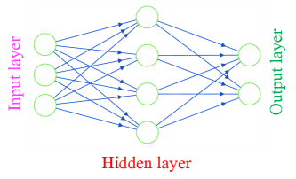
(a) Shallow neural network

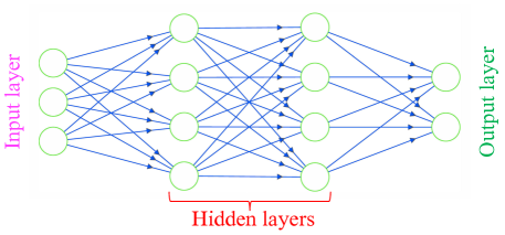
(b) Deep neural network

Fig. 1: Schematic representation of deep and shallow neural networks

Assuming a neural network with $L$ hidden layers, the weighted input into the $i$-th neuron on layer $l$ is represented as

$$z_{i}^{l}=\sigma_{l-1}\left[\sum_{k=1}^{n_{l-1}}\left(W_{i,k}^{l}\cdot z_{k}^{l-1}+b_{i}^{l}\right)\right],$$ (3)

where $W_{i,k}^{l}$ and $b_{i}^{l}$, respectively represent the weights and biases for the selected neuron. $\sigma_{l-1}\left(\bullet\right)$ in Eq. 3 represents the non-linear activation function. It is assumed that the layer $(l-1)$ has $n_{l-1}$ neurons. Note that in the above representation, it is assumed that the $0$-th layer is the input layer and $\left(L+1\right)$-th layer is the output layer. Using Eq. 3, the output response in DNN is represented as

$$\begin{split}\bm{Y}^{L}&=\sigma_{L}(\mathbf{W}^{L+1}\bm{z}^{L}+\bm{b}^{L}),\\ \bm{z}^{L}&=\sigma_{L-1}\left(\mathbf{W}^{L}\bm{z}^{L-1}+\bm{b}^{L}\right),\\ \bm{z}^{L-1}&=\sigma_{L-2}\left(\mathbf{W}^{L-1}\bm{z}^{L-2}+\bm{b}^{L-1}\right),\\ &\vdots\\ \bm{z}^{1}&=\sigma_{0}\left(\mathbf{W}^{1}\bm{\Xi}+\bm{b}^{1}\right).\\ \end{split}$$ (4)

$\bm{Y}$ in Eq. 4 represents the output response. For ease of representation, Eq. 4 can be represented in a more compact form as

$$\bm{Y}=\mathbb{N}\left(\bm{\Xi};\bm{\theta}\right),$$ (5)

where $\mathbb{N}\left(\bullet;\bm{\theta}\right)$ represents the neural network operator with parameters $\bm{\theta}=\left[\mathbf{W},\bm{b}\right]$. For utilizing a neural network in practice, the parameters $\bm{\theta}$ of the neural network needs to be tuned. This is achieved by minimizing some loss-function that force the neural network output to closely match the collected data, $\mathcal{D}=\left\{\bm{\Xi}_{i},\bm{Y}_{i}\right\}_{i=1}^{N_{s}}$. In literature, there exists a plethora of loss-functions. Interested readers can refer [47, 48] to get an account of different loss-functions available in the literature. Since, the DNN discussed above is dependent on data, $\mathcal{D}$, it is referred to as the data-driven DNN.

3.2 From data-driven to physics-informed DNN

Over the years, data-driven DNN has successfully solved a wide range of problems spanning across various domains [49, 50, 51, 52, 53, 54]. Despite such success, one major bottleneck of DNN is its dependence on data; this is particularly true when the data generation process is computationally expensive. To address this issue, the concept of physics-informed deep learning was proposed in [44]. Within this framework, prior knowledge about the model, often available in form of ODE/PDE is utilized to train a DNN model. It was illustrated that this model can solve complex non-linear PDEs.

Consider a nonlinear PDE of the form

$$u_{t}+g\left[u,u_{x},u_{xx},\ldots;\lambda\right]=0,$$ (6)

where $u$ is the unknown solution and $g\left[\bullet;\lambda\right]$ is a nonlinear operator parameterized by $\lambda$. The subscripts in Eq. 6 represents derivative with respect to space and/or time.

$$u_{t}=\frac{\partial u}{\partial t},\;u_{x}=\frac{\partial u}{\partial x},\;u_{xx}=\frac{\partial^{2}u}{\partial x^{2}},\;\cdots$$ (7)

In physics-informed deep learning, the objective is to use Eq. 6 to train a deep neural network model that approximates the unknown variable $u$ in Eq. 6. This is achieved by representing the unknown response $u$ using a neural network

$$u(x,t)\approx\hat{u}(x,t)=\mathbb{N}\left(x,t;\bm{\theta}\right),$$ (8)

and following four simple steps

• Generate a set of collocation points $\mathcal{D}_{c}=\left\{x_{i},t_{i}\right\}_{i=1}^{N_{c}}$, where $N_{c}$ is the number of collocation points generated. Also generate input data corresponding to the boundary and initial conditions, $\mathcal{D}_{b}=\left\{x_{b},t_{i}\right\}_{i=1}^{N_{b}}$ and $\mathcal{D}_{i}=\left\{x_{i},t_{0}\right\}_{i=1}^{N_{i}}$. $N_{b}$ and $N_{i}$ respectively represents the number of points corresponding to boundary condition and initial condition. $t_{0}$ is the initial time and $x_{b}$ is the coordinate where the boundary condition is imposed.

• Based on the generated collocation points, a physics-informed loss-function is formulated as

  $$\mathcal{L}_{p}=\frac{1}{N_{c}}\sum_{i=1}^{N_{c}}\left(R(x_{i},t_{i})\right)^{2},$$ (9)

  where

  $$R(x_{i},t_{i})=\hat{u}_{t}(x_{i},t_{i})+g\left(\hat{u}(x_{i},t_{i}),\hat{u}_{x}((x_{i},t_{i}),\hat{u}_{xx}(x_{i},t_{i}),\ldots;\lambda\right)$$ (10)

  is the residual of the PDE calculated at $(x_{i},t_{i})$. $\hat{u}$ in Eq. 10 is a DNN and is parameterized by $\bm{\theta}$. The derivatives of $\hat{u}_{t}(x_{i},t_{i})$, i.e, $\hat{u}_{x}(x_{i},t_{i})$, $\hat{u}_{xx}(x_{i},t_{i})$ etc are calculated by using AD.

• For the boundary and initial conditions, formulate a data-driven loss-functions

  $$\mathcal{L}_{b}=\frac{1}{N_{b}}\sum_{k=1}^{N_{b}}\left[u_{b,k}-\hat{u}(x_{k},t_{k})\right]^{2},$$ (11a)

  $$\mathcal{L}_{i}=\frac{1}{N_{i}}\sum_{k=1}^{N_{i}}\left[u_{i,k}-\hat{u}(x_{k},t_{k})\right]^{2}.$$ (11b)

  $u_{i,k}$ and $u_{b,k}$ in Eq. 11 represent the initial and boundary conditions of the problem. $\hat{u}$ as before is a DNN.

• Formulate the combined loss-function, $\mathcal{L}$

  $$\mathcal{L}=\mathcal{L}_{p}+\mathcal{L}_{b}+\mathcal{L}_{i},$$ (12)

  and minimize it to obtain the parameters, $\bm{\theta}$.

Once the model is trained, it is used, as usual, to make predictions at unknown point ${x^{*},t^{*}}$.

3.3 Proposed approach

In this section, the physics-informed DNN presented in Section 3.2 is extended for solving reliability analysis problems. Consider, the limit-state function $\mathcal{J}(\bm{\xi})$ discussed in Section 2 is represented as

$$\mathcal{J}(\xi)=u(\xi)-u_{0},$$ (13)

where $u(\xi)$ is the response and $u_{0}$ indicates the threshold value. Also assume that $u(\xi)$ is obtained by solving a stochastic PDE of the form

$$u_{t}+g\left[u,u_{x},u_{xx},\ldots;\xi\right]=0.$$ (14)

Note that Eq. 14 is assumed to have the same functional form as Eq. 6; the only difference is that the parameter $\lambda$ is replaced with $\xi$. This indicates that parameters are considered to be stochastic. With this setup, the objective now is to train a DNN that can act as a surrogate to the response $u$. In a conventional data-driven setup, one first generate training samples from the stochastic input, $\xi_{i},\,i=1,\ldots,N_{s}$, runs a PDE solver such as finite element (FE) method $N_{s}$ times to generate outputs, $u_{i},\,i=1,\ldots,N_{s}$ and then train a data-driven DNN model. Because of the need to run $N_{s}$ FE simulations, such a data-driven approach can quickly become computationally prohibitive for systems defined by complex nonlinear PDEs. This paper takes a different route and attempts to directly develop a DNN based surrogate from the stochastic PDE in Eq. 14. To that end, the stochastic response is first represented in form of a DNN

$$u(x,t,\xi)\approx u_{NN}(x,t,\xi)=\mathbb{N}\left(x,t,\xi;\bm{\theta}\right).$$ (15)

Note that unlike Eq. 8, the input to the neural network now also includes the system parameters, $\xi$. Next, the neural network output is modified to automatically satisfy the initial and/or boundary conditions,

$$\hat{u}\left(x,t,\xi\right)=u_{b,i}(x_{b},t_{i})+B\cdot u_{NN}(x,t,\xi).$$ (16)

The function $B$ is defined in such as way so that $B=0$ at the boundary and initial points. The function $u_{b,i}(x_{b},t_{i})$, on the other hand, is defined using the initial and boundary conditions of the problem. For example, if the boundary condition demands at $x=0$, $u=0$ and the initial condition demands at $t=0$, $u=0$, one sets

$$\hat{u}(x,t,\xi)=x\cdot t\cdot u_{NN}(c,t,\xi).$$ (17)

More examples on how the initial and boundary conditions are automatically satisfied are provided in Section 4. Note that $\hat{u}(x,t,\xi)$ in Eq. 16 can also be viewed as a neural network, $\hat{\mathbb{N}}(x,t,\xi;\bm{\theta})$ with the same parameters $\bm{\theta}$. The derivatives present in PDE are calculated from $\hat{\mathbb{N}}(x,t,\xi;\bm{\theta})$, by using AD.

$$\begin{split}u_{t}\approx\frac{\partial\hat{u}}{\partial t}&=\hat{\mathbb{N}}^{t}(x,t,\xi;\bm{\theta}),\\ u_{x}\approx\frac{\partial\hat{u}}{\partial x}&=\hat{\mathbb{N}}^{x}(x,t,\xi;\bm{\theta}),\\ u_{xx}\approx\frac{\partial^{2}\hat{u}}{\partial x^{2}}&=\hat{\mathbb{N}}^{xx}(x,t,\xi;\bm{\theta}),\\ &\vdots\end{split}$$ (18)

Note that all the derivatives computed in Eq. 18 are deep neural networks with the same exact architecture and parameters and hence, have been denoted using $\hat{\mathbb{N}}^{t}(\cdot,\cdot,\cdot;\bm{\theta})$, $\hat{\mathbb{N}}^{x}(\cdot,\cdot,\cdot;\bm{\theta})$ and $\hat{\mathbb{N}}^{x}x(\cdot,\cdot,\cdot;\bm{\theta})$. The only difference between the original DNN, $\hat{\mathbb{N}}(\cdot,\cdot,\cdot;\bm{\theta})$ and those derived in Eq. 18 resides in the form of the activation function. Using DNNs, the residual of the PDE is defined as

$$R=\hat{\mathbb{N}}^{t}(x,t,\xi;\bm{\theta})+g\left[\hat{\mathbb{N}}(x,t,\xi;\bm{\theta}),\hat{\mathbb{N}}^{x}(x,t,\xi;\bm{\theta}),\hat{\mathbb{N}}^{xx}(x,t,\xi;\bm{\theta}),\ldots\right]=\hat{\mathbb{N}}^{R}(x,t,\xi;\bm{\theta})$$ (19)

Again, the operations carried out in Eq. 19 yields a DNN $\hat{\mathbb{N}}^{R}(\cdot,\cdot,\cdot;\bm{\theta})$ having the same parameters $\bm{\theta}$. When trained, $\hat{\mathbb{N}}^{R}(\cdot,\cdot,\cdot;\bm{\theta})$ ensures that the stochastic PDE is satisfied and hence, is referred to as the physics-informed DNN. In the ideal scenario, $\hat{\mathbb{N}}^{R}(x,t,\xi;\bm{\theta})=0:\xi\in\Omega_{\xi},x\in\Omega_{x},t\in\Omega_{t}$.

To train the network and compute the parameters, $\bm{\theta}$, three simple steps are followed.

• Generate collocation points, $\mathcal{D}=\left\{x_{i},t_{i},\xi_{i}\right\}_{i=1}^{N_{c}}$ are generated by using some suitable DOE scheme.

• Formulate the loss-function as

  $$\mathcal{L}(\bm{\theta})=\frac{1}{N_{c}}\sum_{k=1}^{N_{c}}\left[\hat{\mathbb{N}}^{R}(x_{k},t_{k},\xi_{k};\bm{\theta})^{2}\right].$$ (20)

• Compute $\bm{\theta}$ by minimizing the loss-function

  $$\bm{\theta}^{*}=\arg\min_{\bm{\theta}}\mathcal{L}(\bm{\theta}).$$ (21)

Once the parameters $\bm{\theta}$ has been estimated, $\hat{\mathbb{N}}(x,t,\xi;\bm{\theta})$ (i.e., Eq. 16) can be used to predict response at any unknown point $(x^{*},t^{*},\xi^{*})$. The framework proposed is coded using TensorFlow [55]. For minimizing the loss-function, RMSprop optimizer [56] followed by L-BFGS has been used. Details on parameters of the optimizers are provided in Section 4. A schematic representation of the proposed framework is shown in Fig. 2.

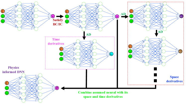
Fig. 2: Proposed physics-informed DNN based framework for simulation free reliability analysis. Along with the spatial and temporal coordinates, the stochastic parameter is also an input to the DNN. All the required derivatives are taken by using automatic differentiation.

The proposed approach has a number of advantages.

• The primary bottleneck in reliability analysis is the need for running computationally expensive simulations. The proposed eliminates this bottleneck as it needs no simulations.

• Since the proposed approach trains the DNN model from the governing PDE/ODE, the solution obtained using the trained model satisfies physical laws such as invariances and conservation laws.

• Unlike most of the methods, the proposed approach provides a continuous solution; the response $u$ can be evaluated at any given point in time and space. This will be extremely helpful in solving time-dependent reliability analysis problems.

4 Numerical illustration

Numerical examples are presented in this section to illustrate the performance of the proposed approach. The examples selected involve a wide variety of problems with limit-state functions defined using ODE and PDE, single equation and system of equations, linear and nonlinear ODE/PDE, and also univariate and multivariate problems. The computational complexity of the problems selected are not high; this enables generating solution using MCS and other state-of-the-art reliability analysis methods for comparison. The software accompanying the proposed approach is developed in python using TensorFlow [55]. For generating the benchmark solutions, MATLAB [57] has been used.

4.1 Ordinary differential equation

As the first example, a simple stochastic ODE is considered.

$$\frac{\text{d}u}{\text{d}t}=-Zu,$$ (22)

where $Z$ is the decay rate coefficient and is considered to be stochastic. The ODE in Eq. 22 is subjected to the following initial condition,

$$u(t=0)=u_{0},$$ (23)

The exact solution for this problem is known.

$$u\left(t,Z\right)=u_{0}\exp\left(-Zt\right).$$ (24)

For reliability analysis, a limit-state function is defined as

$$\mathcal{J}(u\left(t,Z\right))=u\left(t,Z\right)-u_{d},$$ (25)

where $u_{d}$ is the threshold value. This problem has previously been studied in [58].

For this particular example, the stochastic variable $Z\sim\mathcal{N}\left(\mu,\sigma^{2}\right)$ is considered to be following normal distribution with mean, $\mu=-2$ and the standard deviation, $\sigma=1$. The threshold value, $u_{d}=0.5$, and the initial value, $u_{0}=1.0$ is considered. The exact failure probability for this problem is $P_{f}=0.003539$. MCS with $10^{6}$ simulations yields a failure probability of $P_{f}=0.03496$.

For solving the problem using the proposed simulation free reliability analysis framework, the unknown $u$ is represented using a FC-DNN with 2 hidden layers, with each hidden layer having 50 neurons. The DNN has 2 inputs, time $t$ and the stochastic parameter $Z$. The activation function for all but the last layer is considered to be a hyperbolic tangent function (tanh). For the last layer, a linear activation is used. To automatically satisfy the initial condition, the DNN output is modified as

$$\hat{u}=t\cdot u_{NN}+u_{0},$$ (26)

where $u_{0}=1.0$ and $u_{NN}$ is the DNN output. The residual for formulating the loss-function is represented as

$$R_{i}=\frac{\text{d}\hat{u}}{\text{d}t}+Z\hat{u},$$ (27)

where $\hat{u}$ is obtained from Eq. 26. For training the model, 4000 collocation points have been generated using the Latin hypercube sampling [59]. Th RMSprop optimizer is run for 10,000 iterations. The maximum allowable iterations for the L-BFGS optimizer is set to 50,000.

The results obtained using the proposed approach and MCS are shown in Table 1. Reliability index $\beta$ is also computed,

$$\beta=\Phi^{-1}(1-P_{f}),$$ (28)

where $\Phi(\bullet)$ is the cumulative distribution function of standard normal distribution. The results obtained using the proposed approach is found to closely match the exact solutions and MCS results. For sake of comparison, results using FORM, SORM, IS, SS and DS have also been reported in Table 1. All the other methods are found to yield results with similar kind of accuracy. As for efficiency, FORM, SORM, IS, DS and SS requires 42, 44, 1000, 7833 and 1199 simulations, respectively. The proposed approach, on the other hand, needs no simulation for generating the probability of failure estimates.

Table 1: Reliability analysis results for the stochastic ODE problem using various methods.

Methods	$P_{f}$	$\beta$	$N_{s}$	$\epsilon=\frac{\left|\beta_{e}-\beta\right|}{\beta_{e}}$
Exact	$0.003539$	$2.6932$	–	–
MCS	$0.0035$	$2.6949$	$10^{6}$	0.06%
FORM	$0.0036$	$2.6874$	$42$	0.21%
SORM	$0.0036$	$2.6874$	$44$	0.21%
IS	0.0034	$2.7074$	$1000$	0.52%
DS	0.0034	$2.7074$	$7833$	0.52%
SS	$0.0030$	$2.7456$	$1199$	1.95%
PI-DNN	$0.0035$	$2.6949$	$0$	0.06%

To further analyze the performance of the proposed method, systematic case studies by varying the number of neurons, number of hidden layers and the number of collocation points have been carried out. Table 2 reports the reliability index and probability failures obtained corresponding to different settings of the PI-DNN. For this particular problem, the effect of number of hidden layers and number of neurons is relatively less; results corresponding to all the settings are found to be accurate.

Table 2: Variation in reliability analysis results due to change in the DNN architecture (number of hidden layers and neurons). The numbers in the bracket indicates reliability indices.

	30	40	50	60
2	0.00344 (2.7026)	0.0036 (2.6874)	0.00352 (2.6949)	0.00359 (2.6884)
3	0.0037 (2.6783)	0.0036 (2.6874)	0.0036 (2.6874)	0.0036 (2.6874)
3	0.00357 (2.6902)	0.00364 (2.6838)	0.0036 (2.6874)	0.0036 (2.6874)

Table 3 shows the variation in the probability of failure and reliability index estimates with change in the number of collocation points, $N_{c}$. It is observed that the results obtained are more or less constant beyond 500 collocation points. For 250 collocation points, the results obtained are found to be less accurate. Nonetheless, it is safe to conclude that for this problem, results obtained using the proposed PI-DNN based simulation free method is highly accurate.

Table 3: Reliability analysis results with change in number of collocation points.

$N_{c}$	250	500	1000	2000	4000	6000	8000	10000
$P_{f}$	0.00394	0.0035	0.0035	0.0035	0.00352	0.00352	0.00352	0.00352
$\beta$	2.6572	2.6968	2.6968	2.6968	2.6949	2.6949	2.6949	2.6949

4.2 Viscous Burger’s equation

As the second example, viscous Burger’s equation is considered. The PDE of the Burger’s equation is given as

$$u_{t}+uu_{x}=\nu u_{xx},\;\;\;x\in[-1,1],$$ (29)

where $\nu>0$ is the viscosity of the system. The Burger’s equation in Eq. 29 is subjected to the following boundary conditions

$$u(x=-1)=1+\delta\;\;u(x=1)=-1.$$ (30)

The initial condition of the system is obtained by linear interpolation of the boundary conditions.

$$u(t=0,x)=-1+\left(1-x\right)\left(1+\frac{\delta}{2}\right).$$ (31)

$\delta$ in Eqs. 30 and 31 denotes a small perturbation that is applied to the boundary at $x=-1$. Solution of Eq. 29 has a transition layer at distance $z$ such that, $u(z)=0$. As already established in a number of previous studies [60, 61], the location of the transition layer $z$ is super sensitive to the perturbation $\delta$. A detailed study on properties of this transition layer can be found in [60].

In this paper, the perturbation $\delta$ is considered to be a uniformly distributed variable, $\delta\sim\mathcal{U}\left(0,e\right),\;e<<1$. With this the limit-state function is defined as

$$\mathcal{J}\left(z(\delta)\right)=-z(\delta)+z_{0},$$ (32)

where $z_{0}$ is the threshold. For this problem, $e=0.1$ is considered. Different case studies are performed by varying the threshold parameter, $z_{0}$.

For solving this problem using the proposed approach, the unknown variable $u$ is first represented by using a FC-DNN. The FC-DNN considered has 4 hidden layers with each layer having 50 neurons. The DNN has three inputs, the spatial coordinate $x$, the temporal coordinate $t$ ad the stochastic variable $\delta$. Similar to previous example, the activation function of all but the last layer is considered to be tanh, and for the last layer, a linear activation function is considered. To automatically satisfy the boundary and the initial condition, the neural network output $u_{NN}$ is modified as follows.

$$\hat{u}=(1-x)(1+x)tu_{NN}+u(t=0,x),$$ (33)

where $u(t=0,x)$ is defined in Eq. 31. The residual for formulating the physics-informed loss-function is defined as

$$R_{i}=\left.u_{t}\right|_{x=x_{i},t=t_{i},\delta=\delta_{i}}+\left.uu_{x}\right|_{x=x_{i},t=t_{i},\delta=\delta_{i}}-\left.\nu u_{xx}\right|_{x=x_{i},t=t_{i},\delta=\delta_{i}}.$$ (34)

For training the network, 30,000 collocation points have been generated using the Latin hypercube sampling. The RMSProp optimizer is run for 15,000 iterations. The maximum number of allowed iterations for the L-BFGS optimizer is set at 50,000.

For generating benchmark solutions, the deterministic Burger’s equation is solved using FE in FENICS [62]. The FENICS based solver is then coupled with MATLAB based FERUM software [63] for generating the benchmark solutions. Note that the proposed PI-DNN based approach needs no simulation data and hence, no such solver is needed; instead, the PI-DNN is directly trained based on the physics of the problem.

The results obtained using the proposed approach and other state-of-the art methods from the literature are shown in Table 4. The threshold value $z_{0}$ is set to be 0.45 and the reliability analysis is carried out at $t=10$. It is observed that the proposed approach yields highly accurate results, almost matching with the MCS solution. Results obtained using the other methods are slightly less accurate. As for computational efficiency, the MCS results are obtained by running the FE solver 10,000 times. IS, DS, SS, FORM and SORM, respectively needs 1000, 4001, 1000, 58 and 60 runs of the FE solver. The proposed approach, on the other hand, needs no simulations.

Table 4: Reliability analysis results for viscous Burger’s problem.

Methods	$P_{f}$	$\beta$	$N_{s}$	$\epsilon=\frac{\left|\beta_{e}-\beta\right|}{\beta_{e}}$
MCS	0.1037	1.2607	10,000	–
FORM	0.1091	1.2313	58	2.33%
SORM	0.1091	1.2313	60	2.33%
IS	0.1126	1.2128	1000	3.80%
DS	0.0653	1.5117	4001	19.9%
SS	0.0800	1.4051	1000	11.45%
PI-DNN	0.0999	1.2821	0	1.70 %

Next, the performance of the proposed PI-DNN in predicting the reliability corresponding to different thresholds is examined. Through this, it is possible to examine whether the proposed approach is able to emulate the FE solver properly. The results obtained are shown in Fig. 3. Results corresponding to MCS are also shown. It is observed that the proposed approach is able to predict the reliability index corresponding to all the thresholds. This indicates that the DNN, trained only from the governing PDE, is able to reasonably emulate the actual FE solver.

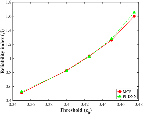
Fig. 3: Reliability index corresponding to different thresholds $z_{0}$ using MCS and PI-DNN.

Lastly, the effect of network architecture and number of collocation points on the performance of the proposed approach is examined. Table 5 shows the results corresponding to different number of collocation points. It is observed that the results improve with increase in the number of collocation points. Beyond 30,000 collocation points, the results is found to stabilize with no significant change.

Table 5: Performance of PI-DNN with change in number of collocation points.

	5000	15000	20000	25000	30000	35000
0.45	0	0	0.0697	0.0791	0.0999	0.1001
0.40	0	0.1064	0.1802	0.1893	0.2058	0.2059
0.35	0.0852	0.2361	0.2858	0.2928	0.3050	0.3051

Tables 6 and 7 show the probability of failure and reliability index estimates corresponding to different number of hidden layers and neurons. It is observed that with too few layers/neurons, the DNN is unable to track the probability of failure. On the other hand, too many neurons/layers results in over-fitting. One way to address this over-fitting issue is to use some form of regularizer in the loss-function. However, this is not within the scope of the current work.

Table 6: Variation in reliability analysis results due to change in number of neurons and number of hidden layers. $z_{0}=0.40$ is considered. The numbers in the bracket indicates reliability index.

	40	50	60
2	0.0 ($\infty$)	0.0 ($\infty$)	0.0 ($\infty$)
3	0.0584 (1.5683)	0.1318 (1.1179)	0.19 (0.8779)
4	0.1741 (0.9380)	0.2058 (0.9380)	0.1721 (0.9459)
5	0.1918 (0.8713)	0.1924 (0.8691)	0.1857 (0.8939)
6	0.1795 (0.9173)	0.1723 (0.9451)	0.19 (0.8779)

Table 7: Variation in reliability analysis results due to change in number of neurons and number of hidden layers. $z_{0}=0.45$ is considered. The numbers in the bracket indicates reliability index

	40	50	60
2	0.0 ($\infty$)	0.0 ($\infty$)	0.0 ($\infty$)
3	0.0 ($\infty$)	0.0 ($\infty$)	0.0836 (1.3813)
4	0.0598 (1.5565)	0.0999 (1.2821)	0.056 (1.5893)
5	0.0759 (1.4332)	0.0855 (1.3690)	0.0741 (1.4459)
6	0.0732 (1.4524)	0.0587 (1.5658)	0.0699 (1.4765)

4.3 Systems of equations: cell-signalling cascade

As the final example of this paper, a mathematical model of the autocrine cell signalling cascade is considered. This model was first proposed in [64]. Considering, $e_{1p}$, $e_{2p}$ and $e_{3p}$ to be the concentrations of the active form of enzymes, the governing differential equations for this system is given as

$$\begin{split}\frac{\text{d}e_{1p}}{\text{d}t}&=\frac{I(t)}{1+G_{4}e_{3p}}\frac{V_{\max,1}(1-e_{1p})}{K_{m,1}+\left(1-e_{1p}\right)}-\frac{V_{\max,2}e_{1p}}{K_{m,2}+e_{1p}},\\ \frac{\text{d}e_{2p}}{\text{d}t}&=\frac{V_{\max,3}e_{1p}(1-e_{2p})}{K_{m,3}+\left(1-e_{2p}\right)}-\frac{V_{\max,4}e_{2p}}{K_{m,4}+e_{2p}},\\ \frac{\text{d}e_{3p}}{\text{d}t}&=\frac{V_{\max,5}e_{2p}(1-e_{3p})}{K_{m,5}+\left(1-e_{3p}\right)}-\frac{V_{\max,6}e_{3p}}{K_{m,6}+e_{3p}},\end{split}$$ (35)

where $G_{4}=0$, $I(t)=1$ and $K_{m,i}=0.2,\,\forall i$. The ODEs in Eq. 35 are subjected to the initial condition,

$$e_{1p}(t=0)=0,\;e_{2p}(t=0)=1,\;e_{3p}(t=0)=0.$$ (36)

The parameters $V_{\max,i},\,i=1,\ldots,6$ are considered to be stochastic. This is a well-known benchmark problem previously studied in [58].

For this problem, $V_{\max,i}$ is defined as

$$V_{\max,i}=\left<V\right>_{\max,i}\left(1+\sigma Z_{i}\right),\;i=1,\ldots,6,$$ (37)

where $\sigma=0.1$. The variable $Z_{i}$ accounts for the uncertainty in $V_{\max,i}$. It is assumed that $Z_{i}\sim\mathcal{U}(-1,1)$ is uniformly distributed with lower-limit $-1$ and upper-limit 1. Therefore this problem has six stochastic variables.

The limit-state function for this problem is defined as

$$\mathcal{J}(Z,t)=e_{3p}(Z,t)-e_{3p,0},$$ (38)

where $e_{3p,0}$ is the threshold value. Similar to Section 4.2, results corresponding to to different threshold values are presented.

For solving the problem using the proposed PI-DNN based simulation free approach, a FC-DINN with four hidden layers is considered. Each hidden layer has 50 neurons. There are seven inputs to the DNN, the six stochastic variables, $Z_{i}$, $=1,\ldots,6$ and time $t$. There are three outputs, $e_{1p}$, $e_{2p}$ and $e_{3p}$. Similar to the previous two examples, the tanh activation function for all but the last layer is considered. For the last layer, linear activation function is used. The neural network output are modified as follows to automatically satisfy the initial conditions.

$$\hat{e}_{1p}=t\cdot e_{1p,NN},\;\;\hat{e}_{2p}=t\cdot e_{2p,NN}+1.0,\;\;\hat{e}_{3p}=t\cdot e_{3p,NN}$$ (39)

where $e_{ip,NN},\,i=1,2,3$ is the raw output from the neural network. The residuals for formulating the loss function are defined as

$$\begin{split}R_{1,i}&=(1+G_{4}\hat{e}_{3p})(K_{m,1}+\left(1-\hat{e}_{1p}\right))(K_{m,2}+\hat{e}_{1p})\frac{\text{d}\hat{e}_{1p}}{\text{d}t}-I(t)(V_{\max,1}(1-\hat{e}_{1p}))(K_{m,2}+\hat{e}_{1p})\\ &+(V_{\max,2}\hat{e}_{1p})(1+G_{4}\hat{e}_{3p})(K_{m,1}+\left(1-\hat{e}_{1p}\right)),\\ R_{2,i}&=(K_{m,3}+\left(1-\hat{e}_{2p}\right))(K_{m,4}+\hat{e}_{2p})\frac{\text{d}\hat{e}_{1p}}{\text{d}t}-(V_{\max,3}\hat{e}_{2p}(1-\hat{e}_{2p}))(K_{m,4}+\hat{e}_{2p})\\ &+(V_{\max,4}\hat{e}_{2p})(K_{m,3}+\left(1-\hat{e}_{2p}\right)),\\ R_{3,i}&=(K_{m,5}+\left(1-\hat{e}_{3p}\right))(K_{m,6}+\hat{e}_{3p})\frac{\text{d}\hat{e}_{2p}}{\text{d}t}-(V_{\max,5}\hat{e}_{2p}(1-\hat{e}_{3p}))(K_{m,6}+\hat{e}_{3p})\\ &+(V_{\max,6}\hat{e}_{3p})(K_{m,5}+\left(1-\hat{e}_{3p}\right)).\\ \end{split}$$ (40)

The dependence of the residuals and the DNN on the collocation points have been removed from brevity of representation. The functional form of residuals presented in Eq. 40 are obtained by carrying out some trivial algebraic operation on the governing equations in Eq. 35; this is necessary to stop the PI-DNN weights from exploding during the training phase. Using the residuals in Eq. 40, the physics-informed loss function for training the PI-DNN is represented as

$$\mathcal{L}=\frac{1}{N_{c}}\sum_{k=1}^{N_{c}}\left(R_{1,k}^{2}\right)+\frac{1}{N_{c}}\sum_{k=1}^{N_{c}}\left(R_{2,k}^{2}\right)+\frac{1}{N_{c}}\sum_{k=1}^{N_{c}}\left(R_{3,k}^{2}\right),$$ (41)

where $N_{c}$ is the number of collocation points. For this example, 20,000 collocation points have been used. The RMSprop optimizer is run for 20,000 iterations. For L-BFGS, maximum allowed iteration is set to be 50,000. For generating benchmark solutions, the MATLAB-inbuilt ODE45 function is coupled with FERUM. The proposed PI-DNN, on the other hand, needs no such simulator.

The results obtained using the proposed approach and other state-of-the art methods from the literature are shown in Table 8. The threshold value $e_{3p,0}$ is set to be 0.54 and the reliability is evaluated at $t=5.0$. It is observed that the results obtained using the proposed approach matches exactly with the MCS results. Among the other methods, DS yields the most accurate results followed by SORM. Because of the nonlinear nature of the limit-state function, results obtained using FORM are found to be little bit erroneous. Similar to the previous examples, the number of simulations required using different methods are also presented. FORM, SORM, IS, DS and SS are found to take 112, 139, 1000, 6017 and 1000 runs of the actual solver. The proposed approach, as already mentioned, needs no simulations.

Table 8: Reliability analysis results for cell-signalling cascade problem.

MCS	$P_{f}$	$\beta$	$N_{s}$	$\epsilon=\frac{\left|\beta_{e}-\beta\right|}{\beta_{e}}$
MCS	0.0459	1.6860	10,000	–
FORM	0.0750	1.4390	112	14.65%
SORM	0.0045	1.69	139	0.23%
IS	0.0467	1.6777	1000	0.49%
DS	0.0455	1.6895	6017	0.21%
SS	0.0414	1.7347	1000	2.89%
PI-DNN	0.0459	1.6860	0	0.0%

Similar to Section 4.2, the performance of the proposed PI-DNN in predicting the reliability index corresponding to different thresholds is examined. The results obtained are shown in Fig. 4. Results corresponding to MCS are also shown. For all the thresholds, results obtained using PI-DNN are found to be extremely close to the MCS predicted results. This illustrates that the PI-DNN has accurately tracked the response of the stochastic system.

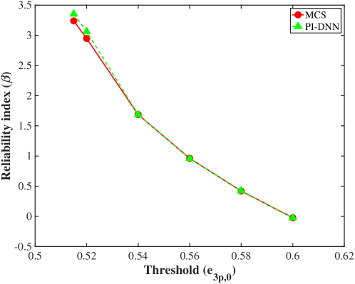
Fig. 4: Reliability index corresponding to different threshold $e_{3p,0}$ obtained using MCS and PI-DNN.

One of the interesting features of the proposed PI-DNN is its ability to predict response at any point in time and space; this is really useful when it comes to solving time-dependent reliability analysis problems. Fig. 5 shows the probability of failure predicted using the proposed PI-DNN at different time-steps. It is observed that the proposed approach yields reasonably accurate results at all the time-step. Note that all the reliability index estimates are obtained by using a single PI-DNN model. This indicates the utility of the proposed PI-DNN in solving time-dependent reliability analysis problems.

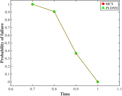
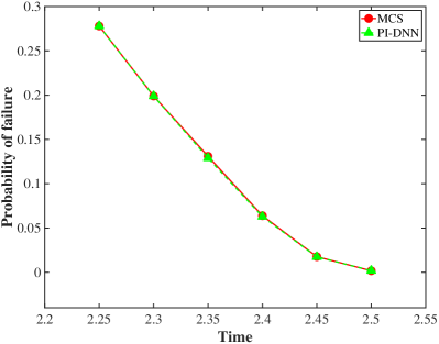
Fig. 5: Probability of failure obtained using the proposed PI-DNN and MCS at different time-instances. $z_{0}$ for (a) is 0.158 and that for (b) is 0.33. The proposed approach is also able to capture small failure probabilities in the order of $10^{-}4$.

Finally, the influence of network architecture and number of collocation points on the performance of the proposed approach is investigated. Table 9 shows the predicted results corresponding to different collocation points. With increase in number of collocation points, the proposed PI-DNN is found to stabilize.

Table 9: Reliability analysis results for cell-signaling cascade problem with change in number of collocation points.

$N_{c}$	5000	10000	15000	20000	30000
$P_{f}$	0.0525	0.0433	0.0435	0.0459	0.0459
$\beta$	1.6211	1.7136	1.7114	1.6860	1.6860

Table 10 shows the results with change in the number of hidden layers and number of neurons. The results obtained are found to be more or less stable with change in the number of hidden layers and neurons

Table 10: Variation in reliability analysis results due to change in number of neurons and number of layers (hidden). The numbers in the bracket indicates reliability index

	40	50	60
2	0.0469 (1.6576)	0.0475 (1.6696)	0.0477 (1.6676)
3	0.0487 (1.6576)	0.0458 (1.6870)	0.0455 (1.6901)
4	0.0469 (1.7018)	0.0459 (1.6860)	0.0458 (1.6870)

5 Conclusions

In this paper, a new class of reliability analysis method that needs no simulation data is proposed. The method proposed is based on recent developments in the field of deep learning and utilizes tools such as automatic differentiation and deep neural networks. Within the proposed framework, the unknown response is represented by using a deep neural network. For obtaining the unknown parameters of the deep neural network, a physics-informed loss function is used. With this loss function, no training data is required and the neural network parameters are directly computed from the governing ODE/PDE of the system. There are three primary advantages of the proposed approach. First, the proposed approach needs no simulation data; this is expected to significantly reduce the computational cost associated with solving a reliability analysis problems. Second, since the network parameters are trained by using a physics-informed loss function, physical laws such as invariances and conservation laws will be respected by the neural network solution. Last but not the least, the proposed approach provides prediction at all spatial and temporal locations and hence, is naturally suited for solving time-dependent reliability analysis problems.

The proposed approach is used for solving three benchmark reliability analysis problems selected from the literature. For all the examples, the proposed approach is found to yield highly accurate results. Comparison carried out with respect to other state-of-the-art reliability analysis methods indicates the suitability of the proposed approach for solving reliability analysis problems. Case studies are carried out to investigate convergence of the proposed approach with respect to number of collocation points and network architecture. The results obtained indicate that the stability and robustness of the proposed approach.

It is to be noted that the approach presented in this paper can further be enhanced in number of ways. For example, replacing the fully connected deep neural network with a convolutional type neural network will possibly enable us to solve really high dimensional reliability analysis problems. Similarly, there is a huge scope to develop adaptive version of this algorithm that will select collocation points in an adaptive manner. The neural network architecture can also be selected by using an adaptive framework. Some of this possibilities will be explored in future studies.

References

- [1] Achintya Haldar and Sankaran Mahadevan. Reliability assessment using stochastic finite element analysis. John Wiley & Sons, 2000.
- [2] Achintya Haldar and Sankaran Mahadevan. Probability, reliability, and statistical methods in engineering design. John Wiley, 2000.
- [3] R Thakur and K B Misra. Monte-Carlo simulation for reliability evaluation of complex systems. International Journal of Systems Science, 9(11):1303–1308, 1978.
- [4] RY. Rubinstein. Simulation and the Monte Carlo method. Wiley, New York, U.S.A., 1981.
- [5] S K Au and J L Beck. A new adaptive importance sampling scheme for reliability calculations. Structural Safety, 21(2):135–158, 1999.
- [6] Bo Li, Thomas Bengtsson, and Peter Bickel. Curse-of-dimensionality revisited: Collapse of importance sampling in very large scale systems. Rapport technique, 85:205, 2005.
- [7] S K Au and J L Beck. Estimation of small failure probabilities in high dimensions by subset simulation. Probabilistic Engineering Mechanics, 16(4):263–277, 2001.
- [8] Siu-Kui Au and Y Wang. Engineering risk assessment with subset simulation. Wiley, 2014.
- [9] Konstantin M. Zuev. Subset simulation method for rare event estimation: an introduction. In Encyclopedia of Earthquake Engineering, pages 1–25. Springer Berlin Heidelberg, Berlin, Heidelberg, 2013.
- [10] O Ditlevsen, R E Melchers, and H Gluver. General multidimensional probability integration by directional simulation. Computers & Structures, 36(2):355–368, 1990.
- [11] M Hohenbichler, S Gollwitzer, W Kruse, and R Rackwitz. New light on first and second order reliability methods. Structural Safety, 4(4):267–284, 1987.
- [12] Yan-Gang Zhao and Tetsuro Ono. A general procedure for first/second-order reliability method (FORM/SORM). Structural Safety, 21(2):95–112, 1999.
- [13] Zhen Hu and Xiaoping Du. First order reliability method for time-variant problems using series expansions. Structural and Multidisciplinary Optimization, 51(1):1–21, 2015.
- [14] Junfu Zhang and Xiaoping Du. A Second-Order Reliability Method With First-Order Efficiency. Journal of Mechanical Design, 132(10):101006, 2010.
- [15] Ikjin Lee, Yoojeong Noh, and David Yoo. A novel second-order reliability method (SORM) using noncentral or generalized Chi-squared distributions. Journal of Mechanical Design, 134(10):100912, 2012.
- [16] Armen Der Kiureghian and Mario De Stefano. Efficient algorithm for second-order reliability analysis. Journal of engineering mechanics, 117(12):2904–2923, 1991.
- [17] Hasan Uǧur Köylüoǧlu and Søren RK Nielsen. New approximations for sorm integrals. Structural Safety, 13(4):235–246, 1994.
- [18] Yan-Gang Zhao and Tetsuro Ono. A general procedure for first/second-order reliabilitymethod (form/sorm). Structural safety, 21(2):95–112, 1999.
- [19] Biswarup Bhattacharyya. A Critical Appraisal of Design of Experiments for Uncertainty Quantification. Archives of Computational Methods in Engineering, 25(3):727–751, 2018.
- [20] Souvik Chakraborty and Rajib Chowdhury. Sequential experimental design based generalised ANOVA. Journal of Computational Physics, 317:15–32, 2016.
- [21] Bruno Sudret. Global sensitivity analysis using polynomial chaos expansions. Reliability Engineering & System Safety, 93(7):964–979, 2008.
- [22] Dongbin Xiu and George Em Karniadakis. The Wiener-Askey polynomial chaos for stochastic differential equations. SIAM Journal on Scientific Computing, 24(2):619–644, 2002.
- [23] Xiu Yang, Minseok Choi, Guang Lin, and George Em Karniadakis. Adaptive ANOVA decomposition of stochastic incompressible and compressible flows. Journal of Computational Physics, 231(4):1587–1614, 2012.
- [24] Souvik Chakraborty and Rajib Chowdhury. Towards ‘h-p adaptive’ generalised ANOVA. Computer Methods in Applied Mechanics and Engineering, 320:558–581, 2017.
- [25] Souvik Chakraborty and Rajib Chowdhury. Modelling uncertainty in incompressible flow simulation using Galerkin based generalised ANOVA. Computer Physics Communications, 208:73–91, 2016.
- [26] Ilias Bilionis and Nicholas Zabaras. Multi-output local Gaussian process regression: Applications to uncertainty quantification. Journal of Computational Physics, 231(17):5718–5746, 2012.
- [27] Souvik Chakraborty and Rajib Chowdhury. Graph-Theoretic-Approach-Assisted Gaussian Process for Nonlinear Stochastic Dynamic Analysis under Generalized Loading. Journal of Engineering Mechanics, 145(12):04019105, 2019.
- [28] Ilias Bilionis, Nicholas Zabaras, Bledar A. Konomi, and Guang Lin. Multi-output separable Gaussian process: Towards an efficient, fully Bayesian paradigm for uncertainty quantification. Journal of Computational Physics, 241:212–239, 2013.
- [29] Rajdip Nayek, Souvik Chakraborty, and Sriram Narasimhan. A Gaussian process latent force model for joint input-state estimation in linear structural systems. Mechanical Systems and Signal Processing, 128:497–530, 2019.
- [30] A. Hosni Elhewy, E. Mesbahi, and Y. Pu. Reliability analysis of structures using neural network method. Probabilistic Engineering Mechanics, 21(1):44–53, 2006.
- [31] J E Hurtado and D A Alvarez. Neural-network-based reliability analysis: a comparative study. Computer Methods in Applied Mechanics and Engineering, 191(1-2):113–132, 2001.
- [32] Hongzhe Dai, Hao Zhang, Wei Wang, and Guofeng Xue. Structural Reliability Assessment by Local Approximation of Limit State Functions Using Adaptive Markov Chain Simulation and Support Vector Regression. Computer-Aided Civil and Infrastructure Engineering, 27(9):676–686, 2012.
- [33] Zhiwei Guo and Guangchen Bai. Application of least squares support vector machine for regression to reliability analysis. Chinese Journal of Aeronautics, 22(2):160–166, 2009.
- [34] Atin Roy and Subrata Chakraborty. Support vector regression based metamodel by sequential adaptive sampling for reliability analysis of structures. Reliability Engineering & System Safety, page 106948, 2020.
- [35] Shyamal Ghosh, Atin Roy, and Subrata Chakraborty. Support vector regression based metamodeling for seismic reliability analysis of structures. Applied Mathematical Modelling, 64:584–602, 2018.
- [36] Roland Schobi, Bruno Sudret, and Joe Wiart. Polynomial-chaos-based kriging. International Journal for Uncertainty Quantification, 5(2), 2015.
- [37] Souvik Chakraborty and Rajib Chowdhury. An efficient algorithm for building locally refined hp–adaptive h-pcfe: Application to uncertainty quantification. Journal of Computational Physics, 351:59–79, 2017.
- [38] Pierric Kersaudy, Bruno Sudret, Nadège Varsier, Odile Picon, and Joe Wiart. A new surrogate modeling technique combining kriging and polynomial chaos expansions–application to uncertainty analysis in computational dosimetry. Journal of Computational Physics, 286:103–117, 2015.
- [39] Souvik Chakraborty and Rajib Chowdhury. Moment independent sensitivity analysis: H-pcfe–based approach. Journal of Computing in Civil Engineering, 31(1):06016001, 2017.
- [40] Somdatta Goswami, Souvik Chakraborty, Rajib Chowdhury, and Timon Rabczuk. Threshold shift method for reliability-based design optimization. Structural and Multidisciplinary Optimization, 60(5):2053–2072, 2019.
- [41] Roland Schöbi, Bruno Sudret, and Stefano Marelli. Rare event estimation using polynomial-chaos kriging. ASCE-ASME Journal of Risk and Uncertainty in Engineering Systems, Part A: Civil Engineering, 3(2):D4016002, 2017.
- [42] Souvik Chakraborty and Rajib Chowdhury. Hybrid framework for the estimation of rare failure event probability. Journal of Engineering Mechanics, 143(5):04017010, 2017.
- [43] Somdatta Goswami, Cosmin Anitescu, Souvik Chakraborty, and Timon Rabczuk. Transfer learning enhanced physics informed neural network for phase-field modeling of fracture. Theoretical and Applied Fracture Mechanics, 106:102447, 2020.
- [44] Maziar Raissi, Paris Perdikaris, and George E Karniadakis. Physics-informed neural networks: A deep learning framework for solving forward and inverse problems involving nonlinear partial differential equations. Journal of Computational Physics, 378:686–707, 2019.
- [45] Yinhao Zhu, Nicholas Zabaras, Phaedon-Stelios Koutsourelakis, and Paris Perdikaris. Physics-constrained deep learning for high-dimensional surrogate modeling and uncertainty quantification without labeled data. Journal of Computational Physics, 394:56–81, 2019.
- [46] Atılım Günes Baydin, Barak A Pearlmutter, Alexey Andreyevich Radul, and Jeffrey Mark Siskind. Automatic differentiation in machine learning: a survey. The Journal of Machine Learning Research, 18(1):5595–5637, 2017.
- [47] Ian Goodfellow, Yoshua Bengio, and Aaron Courville. Deep learning. MIT press, 2016.
- [48] Hagan Demuth Beale, Howard B Demuth, and MT Hagan. Neural network design. Pws, Boston, 1996.
- [49] Yang Xin, Lingshuang Kong, Zhi Liu, Yuling Chen, Yanmiao Li, Hongliang Zhu, Mingcheng Gao, Haixia Hou, and Chunhua Wang. Machine learning and deep learning methods for cybersecurity. IEEE Access, 6:35365–35381, 2018.
- [50] Pinkesh Badjatiya, Shashank Gupta, Manish Gupta, and Vasudeva Varma. Deep learning for hate speech detection in tweets. In Proceedings of the 26th International Conference on World Wide Web Companion, pages 759–760, 2017.
- [51] Adrian Carrio, Carlos Sampedro, Alejandro Rodriguez-Ramos, and Pascual Campoy. A review of deep learning methods and applications for unmanned aerial vehicles. Journal of Sensors, 2017, 2017.
- [52] Xiumin Wang, Jun Li, Hong Chang, and Jinlong He. Optimization design of polar-ldpc concatenated scheme based on deep learning. Computers & Electrical Engineering, 84:106636, 2020.
- [53] Jonathan Waring, Charlotta Lindvall, and Renato Umeton. Automated machine learning: Review of the state-of-the-art and opportunities for healthcare. Artificial Intelligence in Medicine, page 101822, 2020.
- [54] Jean-Baptiste Lamy, Boomadevi Sekar, Gilles Guezennec, Jacques Bouaud, and Brigitte Séroussi. Explainable artificial intelligence for breast cancer: A visual case-based reasoning approach. Artificial intelligence in medicine, 94:42–53, 2019.
- [55] Martín Abadi, Paul Barham, Jianmin Chen, Zhifeng Chen, Andy Davis, Jeffrey Dean, Matthieu Devin, Sanjay Ghemawat, Geoffrey Irving, Michael Isard, et al. Tensorflow: A system for large-scale machine learning. In 12th USENIX Symposium on Operating Systems Design and Implementation (OSDI 16), pages 265–283, 2016.
- [56] Tijmen Tieleman and Geoffrey Hinton. Lecture 6.5-rmsprop: Divide the gradient by a running average of its recent magnitude. COURSERA: Neural networks for machine learning, 4(2):26–31, 2012.
- [57] The Mathworks Inc., Natick, Massachusetts, US. MATLAB and Statistics Toolbox Release 2019b, 2019.
- [58] Jing Li and Dongbin Xiu. Evaluation of failure probability via surrogate models. Journal of Computational Physics, 229(23):8966–8980, 2010.
- [59] R. L. Iman, J. M. Davenport, and D. K. Zeigler. Latin hypercube sampling (program user’s guide). Technical report, Sandia laboratories, 1980.
- [60] Dongbin Xiu and George Em Karniadakis. Supersensitivity due to uncertain boundary conditions. International journal for numerical methods in engineering, 61(12):2114–2138, 2004.
- [61] Jens Lorenz. Nonlinear singular perturbation problems and the Engquist-Osher difference scheme. Katholieke Universiteit Nijmegen. Mathematisch Instituut, 1981.
- [62] Martin Alnæs, Jan Blechta, Johan Hake, August Johansson, Benjamin Kehlet, Anders Logg, Chris Richardson, Johannes Ring, Marie E Rognes, and Garth N Wells. The fenics project version 1.5. Archive of Numerical Software, 3(100), 2015.
- [63] JM Bourinet, C Mattrand, and V Dubourg. A review of recent features and improvements added to ferum software. In Proc. of the 10th International Conference on Structural Safety and Reliability (ICOSSAR’09), 2009.
- [64] Stanislav Yefimovic Shvartsman, Michael P Hagan, A Yacoub, Paul Dent, HS Wiley, and Douglas A Lauffenburger. Autocrine loops with positive feedback enable context-dependent cell signaling. American Journal of Physiology-Cell Physiology, 282(3):C545–C559, 2002.