The Multi-Symplectic Lanczos Algorithm and Its Applications to Color Image Processing

Abstract

Low-rank approximations of original samples are playing more and more an important role in many recently proposed mathematical models from data science. A natural and initial requirement is that these representations inherit original structures or properties. With this aim, we propose a new multi-symplectic method based on the Lanzcos bidiagonalization to compute the partial singular triplets of JRS-symmetric matrices. These singular triplets can be used to reconstruct optimal low-rank approximations while preserving the intrinsic multi-symmetry. The augmented Ritz and harmonic Ritz vectors are used to perform implicit restarting to obtain a satisfactory bidiagonal matrix for calculating the $k$ largest or smallest singular triplets, respectively. We also apply the new multi-symplectic Lanczos algorithms to color face recognition and color video compressing and reconstruction. Numerical experiments indicate their superiority over the state-of-the-art algorithms.

Key words. Multi-symplectic; Lanczos method; Low rank approximation; Face recognition; Video compressing

1 Introduction

The optimal low-rank approximations are the core targets of many recently proposed color image processing models, such as the two dimensional principle component analysis (2DPCA) for color face recognition [18], the robust PCA for color image inpainting [21], and color video compressing and reconstruction [22]. For digital images, we can apply the partial singular value decomposition (SVD) based on the Lanzcos bidiagonalization to reconstruct such low-rank approximations. If the samples have algebraic structures, then the Lanzcos method is expected to be able to preserve these structures which usually reflect the intrinsic relations among different sceneries in the pictures. In this paper, we propose a new multi-symplectic Lanczos bidiagonalization method to preserve the algebraic multi-symmetry of matrices (which represent color images); and the augmented Ritz and harmonic Ritz vector restarting techniques are implicitly applied to obtain the $k$ largest or smallest singular triplets, respectively. This structured Lanczos method will be applied to the color image processing and its own unique advantages will be indicated by numerical experiments.

The Lanczos bidiagonalization method [14, 43] has been widely used to compute the partial singular value decomposition of real or complex matrices of large-scale size. Björck, Grimme and Van Dooren firstly proposed the implicitly restarted technique based on Lanczos bidiagonalization decomposition (LBD) in [6]. Jia and Niu [24] proposed the implicitly restarted LBD with “refined shifts” to calculate partial largest or smallest singular triplets. In order to increase the accuracy of the calculated smallest singular triplets, Kokiopoulou, Bekas, and Gallopoulos [27] proposed the algorithm IRLANB, in which the harmonic Ritz values are used to effectively approximate the smallest singular values. Later, Baglama, and Reichel [1] proposed the algorithms IRLBA(R) and IRLBA(H), by which the $k$ largest or smallest singular triplets of large-scale matrices are obtained from the Ritz vector or harmonic Ritz vector augmented Krylov subspace. In the recent paper [22], the LBD method was generalized to quaternion matrices and the algorithm LANSVDQ was developed to compute the $k$ largest singular triplets and was applied to color face recognition, color video compressing, etc. To the best of our knowledge, there is still no efficient algorithm to compute the $k$ smallest singular triplets of quaternion matrices. The multi-symplectic Lanczos method proposed in this paper can be applied to compute both the $k$ largest singular triplets and the $k$ smallest ones of large-scale quaternion matrices.

The structure-preserving idea is to keep the (algebraic) symmetries or properties of continuous or discrete equations in the solving process. The aim is to accurately, stably and efficiently calculate the required solution. One of the most famous structured matrices in numerous powerful algorithms is the (block) Toeplitz matrix, which is generated in the calculation of differential equations from practical applications, see, e.g., [9, 10, 37, 25, 26]. Another one is the (skew-)Hamiltonian matrix, which arises in the control theory and on which a lot of structure-preserving algorithms and perturbation analysis have been developed [3, 4, 5, 34, 35]. In this paper, we treat an important multi-symmetry, which was firstly proposed in [19], and then widely studied in quaternion computation [20, 22, 30, 31, 45] and in color image processing [18, 21, 23, 32]. This new algebraic symmetry will be preserved in the proposed multi-symplectic Lanczos method. The goal is to combine stability with the speed of actual calculations by performing only real operations.

The rest of this paper is structured as follows. In Section 2, we introduce a new algebraic symmetry and propose the multi-symplectic transformations. In Section 3, we propose a multi-symplectic Lanczos bidiagonalization method for JRS-symmetric matrices and present the restarted multi-symplectic Lanczos method to calculate partial largest or smallest singular triplets of JRS-symmetric matrices. In Section 4, we apply the proposed algorithms to compute partial singular triplets of quaternion matrices and apply it to color image processing. In Section 5, we present numerical examples to demonstrate the efficiency of the proposed algorithms on computing partial singular triplets. In Section 6, we summarize the main work of this paper.

2 Primaries

In this section, we introduce JRS-symmetric matrices and multi-symplectic transformations.

Definition 2.1 (JRS-symmetry [19, 20]).

Define three skew-symmetric matrices as

$$J_{n}=\left[\begin{array}[]{cccc}0&0&-\emph{I}_{n}&0\\ 0&0&0&-\emph{I}_{n}\\ \emph{I}_{n}&0&0&0\\ 0&\emph{I}_{n}&0&0\\ \end{array}\right],~{}R_{n}=\left[\begin{array}[]{cccc}0&-\emph{I}_{n}&0&0\\ \emph{I}_{n}&0&0&0\\ 0&0&0&\emph{I}_{n}\\ 0&0&-\emph{I}_{n}&0\\ \end{array}\right],$$

$$S_{n}=\left[\begin{array}[]{cccc}0&0&0&-\emph{I}_{n}\\ 0&0&\emph{I}_{n}&0\\ 0&-\emph{I}_{n}&0&0\\ \emph{I}_{n}&0&0&0\\ \end{array}\right].$$

A non-zero matrix $M\in\mathbb{R}^{4m\times 4n}$ is called JRS-symmetric if

$$J_{m}MJ_{n}^{T}=R_{m}MR_{n}^{T}=S_{m}MS_{n}^{T}=M.$$ (2)

A matrix $O\in\mathbb{R}^{4m\times 4n}$ is called multi-symplectic if

$$OJ_{n}O^{T}=J_{m},~{}OR_{n}O^{T}=R_{m},~{}OS_{n}O^{T}=S_{m}.$$ (3)

A $JRS$-symmetric matrix $M\in\mathbb{R}^{4m\times 4n}$ has the following algebraic structure,

$$M:=\left[\begin{array}[]{cccc}M^{(0)}&M^{(2)}&M^{(1)}&M^{(3)}\\ -M^{(2)}&M^{(0)}&M^{(3)}&-M^{(1)}\\ -M^{(1)}&-M^{(3)}&M^{(0)}&M^{(2)}\\ -M^{(3)}&M^{(1)}&-M^{(2)}&M^{(0)}\\ \end{array}\right],M^{(i)}\in\mathbb{R}^{m\times n},i=0,1,2,3.$$ (4)

In fact, a real matrix is $JRS$-symmetric if and only if it is a real counterpart of a quaternion matrix [20]. Based on the quaternion representation, a color image with the spatial resolution of $m\times n$ pixels [22] can be represented by an $m\times n$ pure quaternion matrix ${\bf A}$ in $\mathbb{Q}^{m\times n}$ as follows:

$${\bf A}_{ij}=R_{ij}{\bf i}+G_{ij}{\bf j}+B_{ij}{\bf k},\ \ 1\leq i\leq m,1\leq j\leq n,$$

where $R_{ij}$, $G_{ij}$ and $B_{ij}$ are the red, green and blue pixel values at the location $(i,j)$ in the image, respectively, and ${\bf i},{\bf j},{\bf k}$ are three units satisfying ${\bf i}^{2}={\bf j}^{2}={\bf k}^{2}={\bf i}{\bf j}{\bf k}=-1.$ For instance, the color image in Figure 1 can be stored in the quaternion matrix ${\bf A}=R{\bf i}+G{\bf j}+B{\bf k}$, and thus can be represented by the JRS-symmetric matrix

$$A^{(\mathcal{S})}:=\left[\begin{array}[]{rrrr}0&G&R&B\\ -G&0&B&-R\\ -R&-B&0&G\\ -B&R&-G&0\\ \end{array}\right],$$

where

$$R=\left[\begin{array}[]{cccc}0&0&1&0\\ 0&0&0&1\\ 1&0&0&0\\ 0&1&0&0\\ \end{array}\right]\otimes Z,~{}G=\left[\begin{array}[]{cccc}0&1&0&0\\ 0&0&1&0\\ 0&0&0&1\\ 1&0&0&0\\ \end{array}\right]\otimes Z,~{}B=\left[\begin{array}[]{cccc}0&0&0&1\\ 1&0&0&0\\ 0&1&0&0\\ 0&0&1&0\\ \end{array}\right]\otimes Z,$$

represent the red, green, and blue components, respectively, and $Z$ is an $n$-by-$n$ matrix with all entries being ones. Recall that Sir W. Hamilton (1805-1865) invented quaternions in 1843 when he attended to extend a complex number to a higher spatial dimension space[16]. In the contemporary era, quaternions have been well known and widely applied in color image processing [21, 23, 40, 42]. See Section 4 for more details of the application to color image processing.

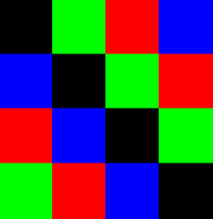
Figure 1: Color image of size $200\times 200$.

The multi-symplectic transformations can preserve the JRS-symmetric structure, which often associates to the practical relationships between considered elements, during the resolvent process. One example is the orthogonally $JRS$-symplectic matrix $W\in\mathbb{R}^{4n\times 4n}$, proposed in [20], having the following form:

$$W:=\left[\begin{array}[]{cccc}W^{(0)}&W^{(2)}&W^{(1)}&W^{(3)}\\ -W^{(2)}&W^{(0)}&W^{(3)}&-W^{(1)}\\ -W^{(1)}&-W^{(3)}&W^{(0)}&W^{(2)}\\ -W^{(3)}&W^{(1)}&-W^{(2)}&W^{(0)}\\ \end{array}\right],W^{(i)}\in\mathbb{R}^{n\times n},i=0,1,2,3.$$

Such a orthogonal and $JRS$-symplectic matrix corresponds to a unitary quaternion matrix [20], and preserves the $JRS$-symmetric structure in a similarity transformation.

The following notation will be used frequently. The superscript $*^{(\mathcal{S})}$ over a matrix $M$, say $M^{(\mathcal{S})}$, indicates that $M$ has the algebraic structure (4). The JRS-symmetric matrix $M^{(\mathcal{S})}$ will be saved by its first block row in the practical implementation, i.e., $M^{(\mathcal{S})}:=[M^{(0)},M^{(2)},M^{(1)},M^{(3)}]$. The block diagonal matrix with diagonal elements, $A_{i}$’s, is denoted by ${\tt diag}(A_{1},A_{2},\cdots,A_{k})$.

3 Multi-Symplectic Lanczos Method

In this section, we present the multi-symplectic Lanczos method for the computation of the $k~{}(k<n)$ largest and smallest singular triplets of a $4n$-by-$4n$ JRS-symmetric matrices. The core work is to calculate a structured bidiagonalization of the form

$$B_{k}^{(\mathcal{S})}={\tt diag}(B_{k},B_{k},B_{k},B_{k}),~{}B_{k}=\left[\begin{array}[]{ccccc}\alpha_{1}&\beta_{1}&0&\cdots&0\\ 0&\alpha_{2}&\beta_{2}&\ddots&0\\ \vdots&\ddots&\ddots&\ddots&\vdots\\ \vdots&\ddots&\ddots&\ddots&\beta_{k-1}\\ 0&\cdots&\cdots&0&\alpha_{k}\\ \end{array}\right]\in\mathbb{R}^{k\times k},$$ (5)

rather than a bidiagonal matrix of size $4k\times 4k$ by the classic Lanczos method.

3.1 Multi-Symplectic Lanczos Bidiagonalization

The multi-symplectic Lanczos bidigonalization method aims to compute the partial bidiagonalization of a JRS-symmetric matrix $M\in\mathbb{R}^{4m\times 4n}$.

At first, we propose the bidigonalization of a JRS-symmetric matrix $M\in\mathbb{R}^{4m\times 4n}$.

Theorem 3.1 (Multi-Symplectic Bidiagonalization Decomposition).

If matrix $M\in\mathbb{R}^{4m\times 4n}$ is $JRS$-symmetric. Then there exist two orthogonally multi-symplectic matrices $P\in\mathbb{R}^{4n\times 4n}$ and $Q\in\mathbb{R}^{4m\times 4m}$ such that

$$M=Q\left[\begin{array}[]{cccc}B&0&0&0\\ 0&B&0&0\\ 0&0&B&0\\ 0&0&0&B\\ \end{array}\right]P^{T},$$ (6)

where $B\in\mathbb{R}^{m\times n}$ is a real bidiagonal matrix.

Proof.

We prove the theorem by induction on the dimension. Clearly, the theorem holds for $m=n=1$. Assume that the result is true for any $4(m-1)\times 4(n-1)$ $JRS$-symmetric matrix.

For any $JRS$-symmetric matrix $M\in\mathbb{R}^{4m\times 4n}$, its four distant blocks are partitioned as

$$M^{(0)}=\left[\begin{array}[]{c|ccc}\omega^{(0)}_{11}&\omega^{(0)}_{12}&\Omega^{(0)}_{13}\\ \hline\cr\omega^{(0)}_{21}&\omega^{(0)}_{22}&\Omega^{(0)}_{23}\\ \Omega^{(0)}_{31}&\Omega^{(0)}_{32}&\Omega^{(0)}_{33}\\ \end{array}\right],\ \ \ \ \ \ M^{(1)}=\left[\begin{array}[]{c|ccc}\omega^{(1)}_{11}&\omega^{(1)}_{12}&\Omega^{(1)}_{13}\\ \hline\cr\omega^{(1)}_{21}&\omega^{(1)}_{22}&\Omega^{(1)}_{23}\\ \Omega^{(1)}_{31}&\Omega^{(1)}_{32}&\Omega^{(1)}_{33}\\ \end{array}\right],$$

$$M^{(2)}=\left[\begin{array}[]{c|ccc}\omega^{(2)}_{11}&\omega^{(2)}_{12}&\Omega^{(2)}_{13}\\ \hline\cr\omega^{(2)}_{21}&\omega^{(2)}_{22}&\Omega^{(2)}_{23}\\ \Omega^{(2)}_{31}&\Omega^{(2)}_{32}&\Omega^{(2)}_{33}\\ \end{array}\right],\ \ \ \ \ \ M^{(3)}=\left[\begin{array}[]{c|ccc}\omega^{(3)}_{11}&\omega^{(3)}_{12}&\Omega^{(3)}_{13}\\ \hline\cr\omega^{(3)}_{21}&\omega^{(3)}_{22}&\Omega^{(3)}_{23}\\ \Omega^{(3)}_{31}&\Omega^{(3)}_{32}&\Omega^{(3)}_{33}\\ \end{array}\right],$$

in which $\omega^{(t)}_{ij}\in\mathbb{R}$, $\Omega^{(t)}_{33}\in\mathbb{R}^{(m-2)\times(n-2)}$, and $\Omega^{(t)}_{i3},(\Omega^{(t)}_{3j})^{T}\in\mathbb{R}^{m-2}$. There exist two muti-symplectic matrices, denoted by $P_{1}\in\mathbb{R}^{4n\times 4n}$ and $Q_{1}\in\mathbb{R}^{4m\times 4m}$ such that

$$\tilde{M}:=Q_{1}MP_{1}^{T}:=\left[\begin{array}[]{cccc}\tilde{{M}}^{(0)}&\tilde{{M}}^{(2)}&\tilde{{M}}^{(1)}&\tilde{{M}}^{(3)}\\ -\tilde{{M}}^{(2)}&\tilde{{M}}^{(0)}&\tilde{{M}}^{(3)}&-\tilde{{M}}^{(1)}\\ -\tilde{{M}}^{(1)}&-\tilde{{M}}^{(3)}&\tilde{{M}}^{(0)}&\tilde{{M}}^{(2)}\\ -\tilde{{M}}^{(3)}&\tilde{{M}}^{(1)}&-\tilde{{M}}^{(2)}&\tilde{{M}}^{(0)}\\ \end{array}\right]$$

where

$$\tilde{{M}}^{(0)}=\left[\begin{array}[]{c|cc}\gamma_{11}&\gamma_{12}&0\\ \hline\cr 0&\tilde{{\omega}}^{(0)}_{22}&\tilde{{\Omega}}^{(0)}_{23}\\ 0&\tilde{{\Omega}}^{(0)}_{32}&\tilde{{\Omega}}^{(0)}_{33}\end{array}\right],\ \ \ \tilde{{M}}^{(1)}=\left[\begin{array}[]{c|cc}0&0&0\\ \hline\cr 0&\tilde{{\omega}}^{(1)}_{22}&\tilde{{\Omega}}^{(1)}_{23}\\ 0&\tilde{{\Omega}}^{(1)}_{32}&\tilde{{\Omega}}^{(1)}_{33}\end{array}\right],$$

$$\tilde{{M}}^{(2)}=\left[\begin{array}[]{c|cc}0&0&0\\ \hline\cr 0&\tilde{{\omega}}^{(2)}_{22}&\tilde{{\Omega}}^{(2)}_{23}\\ 0&\tilde{{\Omega}}^{(2)}_{32}&\tilde{{\Omega}}^{(2)}_{33}\end{array}\right],\ \ \ \tilde{{M}}^{(3)}=\left[\begin{array}[]{c|cc}0&0&0\\ \hline\cr 0&\tilde{{\omega}}^{(3)}_{22}&\tilde{{\Omega}}^{(3)}_{23}\\ 0&\tilde{{\Omega}}^{(3)}_{32}&\tilde{{\Omega}}^{(3)}_{33}\end{array}\right].$$

Here, $\gamma_{11},\gamma_{12}\geq 0$, and $P_{1}$ and $Q_{1}$ are products of a series of generalized Givens transformations defined as in [19],

$$G(i):=\left[\setcounter{MaxMatrixCols}{12}\begin{smallmatrix}\emph{I}_{i-1},&0,&0,&0,&0,&0,&0,&0,&0,&0,&0,&0\\ 0,&\cos\alpha_{0},&0,&0,&\cos\alpha_{2},&0,&0,&\cos\alpha_{1},&0,&0,&\cos\alpha_{3},&0\\ 0,&0,&\emph{I}_{m-i},&0,&0,&0,&0,&0,&0,&0,&0,&0\\ 0,&0,&0,&\emph{I}_{i-1},&0,&0,&0,&0,&0,&0,&0,&0\\ 0,&-\cos\alpha_{2},&0,&0,&\cos\alpha_{0},&0,&0,&\cos\alpha_{3},&0,&0,&-\cos\alpha_{1},&0\\ 0,&0,&0,&0,&0,&\emph{I}_{m-i},&0,&0,&0,&0,&0,&0\\ 0,&0,&0,&0,&0,&0,&\emph{I}_{i-1},&0,&0,&0,&0,&0\\ 0,&-\cos\alpha_{1},&0,&0,&-\cos\alpha_{3},&0,&0,&\cos\alpha_{0},&0,&0,&\cos\alpha_{2},&0\\ 0,&0,&0,&0,&0,&0,&0,&0,&\emph{I}_{m-i},&0,&0,&0\\ 0,&0,&0,&0,&0,&0,&0,&0,&0,&\emph{I}_{i-1},&0,&0\\ 0,&-\cos\alpha_{3},&0,&0,&\cos\alpha_{1},&0,&0,&-\cos\alpha_{2},&0,&0,&\cos\alpha_{0},&0\\ 0,&0,&0,&0,&0,&0,&0,&0,&0,&0,&0,&\emph{I}_{m-i}\\ \end{smallmatrix}\right],$$

where $\alpha_{0},\alpha_{1},\alpha_{2},\alpha_{3}\in[-\pi/2,\pi/2)$ and $\cos^{2}\alpha_{0}+\cos^{2}\alpha_{1}+\cos^{2}\alpha_{2}+\cos^{2}\alpha_{3}=1$.

Denote $M^{\prime}$ as the submatrix of $\tilde{{M}}$ by deleting the $1,m+1,2m+1,3m+1$ rows and the $1,n+1,2n+1,3n+1$ columns. Clearly, $M^{\prime}\in\mathbb{R}^{4(m-1)\times 4(n-1)}$ is $JRS$-symmetric. By the introduction assumption, there exist two orthogonal $JRS$-symplectic matrices,

$$P^{\prime}=\left[\begin{array}[]{cccc}P^{\prime(0)}&P^{\prime(2)}&P^{\prime(1)}&P^{\prime(3)}\\ -P^{\prime(2)}&P^{\prime(0)}&P^{\prime(3)}&-P^{\prime(1)}\\ -P^{\prime(1)}&-P^{\prime(3)}&P^{\prime(0)}&P^{\prime(2)}\\ -P^{\prime(3)}&P^{\prime(1)}&-P^{\prime(2)}&P^{\prime(0)}\\ \end{array}\right]$$

and

$$Q^{\prime}=\left[\begin{array}[]{cccc}Q^{\prime(0)}&Q^{\prime(2)}&Q^{\prime(1)}&Q^{\prime(3)}\\ -Q^{\prime(2)}&Q^{\prime(0)}&Q^{\prime(3)}&-Q^{\prime(1)}\\ -Q^{\prime(1)}&-Q^{\prime(3)}&Q^{\prime(0)}&Q^{\prime(2)}\\ -Q^{\prime(3)}&Q^{\prime(1)}&-Q^{\prime(2)}&Q^{\prime(0)}\\ \end{array}\right]$$

such that

$$(Q^{\prime})^{T}M^{\prime}P^{\prime}=\left[\begin{array}[]{cccc}B^{\prime}&0&0&0\\ 0&B^{\prime}&0&0\\ 0&0&B^{\prime}&0\\ 0&0&0&B^{\prime}\\ \end{array}\right],$$ (7)

in which $B^{\prime}\in\mathbb{R}^{(m-1)\times(n-1)}$ is a bidiagonal matrix. Define

$$P_{2}^{(t)}=\left[\begin{array}[]{cccc}1&0\\ 0&P^{\prime(t)}\\ \end{array}\right]\in\mathbb{R}^{n\times n}~{}\text{and}~{}Q_{2}^{(t)}=\left[\begin{array}[]{cc}1&0\\ 0&Q^{\prime(t)}\\ \end{array}\right]\in\mathbb{R}^{m\times m},~{}t=0,1,2,3.$$

We structure two orthogonal multi-symplectic matrices

$$P_{2}:=\left[\begin{array}[]{cccc}P_{2}^{(0)}&P_{2}^{(2)}&P_{2}^{(1)}&P_{2}^{(3)}\\ -P_{2}^{(2)}&P_{2}^{(0)}&P_{2}^{(3)}&-P_{2}^{(1)}\\ -P_{2}^{(1)}&-P_{2}^{(3)}&P_{2}^{(0)}&P_{2}^{(2)}\\ -P_{2}^{(3)}&P_{2}^{(1)}&-P_{2}^{(2)}&P_{2}^{(0)}\\ \end{array}\right]$$

and

$$Q_{2}:=\left[\begin{array}[]{cccc}Q_{2}^{(0)}&Q_{2}^{(2)}&Q_{2}^{(1)}&Q_{2}^{(3)}\\ -Q_{2}^{(2)}&Q_{2}^{(0)}&Q_{2}^{(3)}&-Q_{2}^{(1)}\\ -Q_{2}^{(1)}&-Q_{2}^{(3)}&Q_{2}^{(0)}&Q_{2}^{(2)}\\ -Q_{2}^{(3)}&Q_{2}^{(1)}&-Q_{2}^{(2)}&Q_{2}^{(0)}\\ \end{array}\right].$$

Then by defining $P=P_{1}P_{2}$ and $Q=Q_{1}Q_{2}$, we have

$$Q^{T}MP=(Q_{1}Q_{2})^{T}MP_{1}P_{2}=\left[\begin{array}[]{cccc}B&0&0&0\\ 0&B&0&0\\ 0&0&B&0\\ 0&0&0&B\\ \end{array}\right],$$ (8)

where

$$B=\left[\begin{array}[]{c|c}\gamma_{11}&[\gamma_{12}~{}0]\\ \hline\cr 0&B^{\prime}\end{array}\right]\in\mathbb{R}^{m\times n}$$

is a bidiagonal matrix. $P$ and $Q$ are surely orthogonally multi-symplectic, since they are products of two orthogonally multi-symplectic matrices. ∎

Next, we propose the multi-symplectic Lanczos bidigonalization (MLB) method to compute the partial bidiagonalization of a JRS-symmetric matrix $M\in\mathbb{R}^{4m\times 4n}$.

Theorem 3.2 (Partial Bidiagonalization Decomposition).

Suppose that $M^{(\mathcal{S})}\in\mathbb{R}^{4m\times 4n}$ is a JRS-symmetric matrix of the form (4) and $1\leq k\leq\min(m,n)$. There exist two multi-symmplectic matrices $P_{k}^{(\mathcal{S})}\in\mathbb{R}^{4n\times 4k}$ and $Q_{k}^{(\mathcal{S})}\in\mathbb{R}^{4m\times 4k}$ with orthogonal columns, such that

$$M^{(\mathcal{S})}P_{k}^{(\mathcal{S})}=Q_{k}^{(\mathcal{S})}B_{k}^{(\mathcal{S})},~{}(M^{(\mathcal{S})})^{T}Q_{k}^{(\mathcal{S})}=P_{k}^{(\mathcal{S})}B_{k}^{(\mathcal{S})}+r_{k}^{(\mathcal{S})}(e_{k}^{(\mathcal{S})})^{T},$$ (9)

where $B_{k}^{(\mathcal{S})}$ is of the form (5) with $\alpha_{j}>0$ and $\beta_{j}\geq 0$, $r_{k}^{(\mathcal{S})}=\texttt{diag}(r_{k},r_{k},r_{k},r_{k})$ $\in\mathbb{R}^{4n\times 4}$ is a “residual vector” satisfying $(P_{k}^{(\mathcal{S})})^{T}r_{k}^{(\mathcal{S})}=0$, and $e_{k}^{(\mathcal{S})}=\texttt{diag}(e_{k},e_{k},e_{k},e_{k})$ $\in\mathbb{R}^{4m\times 4}$ with $e_{k}$ denoting the $k$th column of the identity matrix.

Proof.

With the structure-preserving transformations in hand, we can complete the proof in the similar way to that of Theorem 3.1. ∎

The pseudo-code of the MLB method is proposed in Algorithm 1, in which $\|\cdot\|$ denotes the $Frobenius$ $norm$. To save storage, we use the notation $M^{(\mathcal{S})}$, $P_{k}^{(\mathcal{S})}$ and $Q_{k}^{(\mathcal{S})}$, but only update and save their first block rows.

Notice that we need the reorthogonalization with preserving multi-symplectic structure in lines 5 and 10 since the orthogonality of computed columns is often lost during computation. If without breakdown, we compute matrices $P_{k}^{(\mathcal{S})}$, $Q_{k}^{(\mathcal{S})}$ and $B_{k}^{(\mathcal{S})}$, satisfying Theorem 3.2 . The output matrix $B_{k}$ is a bidiagonal matrix as in (5), $\alpha_{j}>0,\beta_{j}\geq 0,1\leq j\leq k$.

Due to the limitation of computing speed and memory, the value of $k$ should not be too large in practical calculation. However, too small $k$ can not always guarantee the enough accuracy and the convergence of the multi-symplectic Lanczos bidiagonalization algorithm. A useful technique is restarting, which is applied to make the approximate singular triplets converge at the preset accuracy. At present, there are many available restarted strategies. The implicitly restarting technology proposed by Sorensen [44] for eigenvalues is one of the most successful restarting technologies. We will propose the details of applying this technique in Section 3.2.

Algorithm 3.1.

Algorithm 1. The Multi-Symplectic Lanczos (MSL) Bidiagonalization

1. $M^{(\mathcal{S})}\in\mathbb{R}^{m\times 4n}$:  a $JRS$-symmetric matrix,

2. $p_{1}^{(\mathcal{S})}\in\mathbb{R}^{n\times 4}$: “initial vector” satisfies $\|p_{1}^{(\mathcal{S})}\|=1$,

3. $k$: number of bidiagonalization steps.

4. $P_{k}^{(\mathcal{S})}\in\mathbb{R}^{n\times 4k}$: matrix with orthonormal columns,

5. $Q_{k}^{(\mathcal{S})}\in\mathbb{R}^{m\times 4k}$: matrix with orthonormal columns,

6. $B_{k}\in\mathbb{R}^{k\times k}$: upper bidiagonal matrix with entries $\alpha_{j},\beta_{j}$,

7. $r_{k}^{(\mathcal{S})}\in\mathbb{R}^{n\times 4}$: residual vector.

8. $P_{1}^{(\mathcal{S})}:=p_{1}^{(\mathcal{S})};q_{1}^{(\mathcal{S})}:=Mp_{1}^{(\mathcal{S})}$;

9. $\alpha_{1}:=\parallel q_{1}^{(\mathcal{S})}\parallel;q_{1}^{(\mathcal{S})}:=q_{1}^{(\mathcal{S})}/\alpha_{1};Q_{1}^{(\mathcal{S})}:=q_{1}^{(\mathcal{S})};$

10. for $j=1:k$

11. $r_{j}^{(\mathcal{S})}:=(M^{(\mathcal{S})})^{T}q_{j}^{(\mathcal{S})}-\alpha_{j}p_{j}^{(\mathcal{S})};$

12. Reorthogonalization: $r_{j}^{(\mathcal{S})}:=r_{j}^{(\mathcal{S})}-P_{j}^{(\mathcal{S})}((P_{j}^{(\mathcal{S})})^{T}r_{j}^{(\mathcal{S})});$

13. if $j<k,$

14. $\beta_{j}:=\parallel r_{j}^{(\mathcal{S})}\parallel;\ p_{j+1}^{(\mathcal{S})}:=r_{j}^{(\mathcal{S})}/\beta_{j}$;

15. $P_{j+1}^{(\mathcal{S})}:$=$[P_{j}^{(\mathcal{S})}(:,1:j),p_{j+1}^{(\mathcal{S})}(:,1),P_{j}^{(\mathcal{S})}(:,j+1:2j),$ $p_{j+1}^{(\mathcal{S})}(:,2)$, $P_{j}^{(\mathcal{S})}(:,2j+1:3j),$ $p_{j+1}^{(\mathcal{S})}(:,3),P_{j}^{(\mathcal{S})}(:,3j+1:4j),p_{j+1}^{(\mathcal{S})}(:,4)];$

16. $q_{j+1}^{(\mathcal{S})}:=M^{(\mathcal{S})}p_{j+1}^{(\mathcal{S})}-\beta_{j}q_{j}^{(\mathcal{S})}$;

17. Reorthogonalization: $q_{j+1}^{(\mathcal{S})}:=q_{j+1}^{(\mathcal{S})}-Q_{j}^{(\mathcal{S})}(Q_{j}^{(\mathcal{S})})^{T}q_{j+1}^{(\mathcal{S})}$;

18. $\alpha_{j+1}:=\|q_{j+1}^{(\mathcal{S})}\|;\ q_{j+1}^{(\mathcal{S})}:=q_{j+1}^{(\mathcal{S})}/\alpha_{j+1};$

19. $Q_{j+1}^{(\mathcal{S})}:=[Q_{j}^{(\mathcal{S})}(:,1:j),$ $q_{j+1}^{(\mathcal{S})}(:,1),$ $Q_{j}^{(\mathcal{S})}(:,j+1:2j),$ $q_{j+1}^{(\mathcal{S})}(:,2),$ $Q_{j}^{(\mathcal{S})}(:,2j+1:3j),$ $q_{j+1}^{(\mathcal{S})}(:,3),$ $Q_{j}^{(\mathcal{S})}(:,3j+1:4j),q_{j+1}^{(\mathcal{S})}(:,4)];$

20. end

21. end

3.2 Computation of $k$ Largest Singular Triplets

Let the partial Lanczos bidiagonalization (9) be available, and assume that we are interested in determining the $t$ largest singular triplets of $M\in\mathbb{R}^{4m\times 4n}$, where $t\leq k<\min(m,n)$. Let $\{\sigma_{j},u_{j},v_{j}\}$, $j=1,\dots,k$, with

$$\sigma_{1}\geq\sigma_{2}\geq\cdots\geq\sigma_{k}\geq 0,$$

be the singular triplets of $B_{k}$, i.e.,

$$B_{k}v_{j}=u_{j}\sigma_{j},\ B_{k}^{T}u_{j}=v_{j}\sigma_{j}.$$ (10)

To obtain the singular triplets of $M^{(\mathcal{S})}$, we need firstly construct three diagonal or block diagonal matrices as follows:

$$\sigma_{j}^{(\mathcal{S})}=\texttt{diag}(\sigma_{j},\sigma_{j},\sigma_{j},\sigma_{j}),~{}u_{j}^{(\mathcal{S})}=\texttt{diag}(u_{j},u_{j},u_{j},u_{j}),~{}v_{j}^{(\mathcal{S})}=\texttt{diag}(v_{j},v_{j},v_{j},v_{j}).$$ (11)

The right and left singular vectors of $M^{(\mathcal{S})}$ are generated by computing

$$\tilde{u}_{j}^{(\mathcal{S})}=Q_{k}^{(\mathcal{S})}u_{j}^{(\mathcal{S})},~{}\tilde{v}_{j}^{(\mathcal{S})}=P_{k}^{(\mathcal{S})}v_{j}^{(\mathcal{S})}.$$ (12)

Then we finally obtain the Lanczos bidiagonalization of $M^{(\mathcal{S})}$,

$$M^{(\mathcal{S})}\tilde{v}_{j}^{(\mathcal{S})}=\tilde{u}_{j}^{(\mathcal{S})}\sigma_{j}^{(\mathcal{S})},\ (M^{(\mathcal{S})})^{T}\tilde{u}_{j}^{(\mathcal{S})}=\tilde{v}_{j}^{(\mathcal{S})}\sigma_{j}^{(\mathcal{S})}+r_{k}^{(\mathcal{S})}(e_{k}^{(\mathcal{S})})^{T}u_{j}^{(\mathcal{S})},\ 1\leq j\leq k.$$ (13)

So that $\{{\tilde{\sigma}_{j}^{(\mathcal{S})},\tilde{u}_{j}^{(\mathcal{S})},\tilde{v}_{j}^{(\mathcal{S})}}\}$ can be accepted as an approximate singular triplet of $M^{(\mathcal{S})}$ if the Frobenius norm of $r_{k}^{(\mathcal{S})}(e_{k}^{(\mathcal{S})})^{T}u_{j}^{(\mathcal{S})}$ is sufficiently small.

From the partial Lanczos bidigonalization decomposition of $M^{(\mathcal{S})}$, we can exactly deduce the partial Lanczos tridiagonalization of $(M^{(\mathcal{S})})^{T}M^{(\mathcal{S})}$. Indeed, multiplying the first equation of (9) by $(M^{(\mathcal{S})})^{T}$ from the left-hand side and applying the second equation of (9) yields

$$(M^{(\mathcal{S})})^{T}M^{(\mathcal{S})}P_{k}^{(\mathcal{S})}=P_{k}^{(\mathcal{S})}(B_{k}^{(\mathcal{S})})^{T}B_{k}^{(\mathcal{S})}+\alpha_{k}r_{k}^{(\mathcal{S})}(e_{k}^{(\mathcal{S})})^{T}.$$ (14)

The columns of $P_{k}^{(\mathcal{S})}$ are separated into four independent groups which satisfy the three-term recurrence relationship. This can be seen from

$$T_{k}^{(\mathcal{S})}:=(B_{k}^{(\mathcal{S})})^{T}B_{k}^{(\mathcal{S})}\\ =\texttt{diag}(T_{k},T_{k},T_{k},T_{k}),$$

where

$$T_{k}:=B_{k}^{T}B_{k}=\left[\begin{array}[]{ccccc}\alpha_{1}^{2}&\beta_{1}\alpha_{1}&0&\cdots&0\\ \beta_{1}\alpha_{1}&\alpha_{2}^{2}+\beta_{1}^{2}&\beta_{2}\alpha_{3}&\cdots&0\\ 0&\ddots&\ddots&\ddots&0\\ 0&0&\ddots&\alpha_{k-1}^{2}+\beta_{k-2}^{2}&\beta_{k-2}\alpha_{k}\\ 0&0&\cdots&\beta_{k-2}\alpha_{k}&\alpha_{k}^{2}+\beta_{k-1}^{2}\\ \end{array}\right]\in\mathbb{R}^{k\times k}.$$

Define $p_{j}^{(\mathcal{S})}:=P_{k}^{(\mathcal{S})}e_{j}^{(\mathcal{S})}$, $j=1,\ldots,k$. Then {$p_{1}^{(\mathcal{S})}$, $p_{2}^{(\mathcal{S})}$, …, $p_{k}^{(\mathcal{S})}$} acts as an orthonormal basis of the block Krylov subspace

$$\mathcal{K}((M^{(\mathcal{S})})^{T}M^{(\mathcal{S})},p_{1}^{(\mathcal{S})})=\texttt{span}\{p_{1}^{(\mathcal{S})},(M^{(\mathcal{S})})^{T}M^{(\mathcal{S})}p_{1}^{(\mathcal{S})},\cdots,((M^{(\mathcal{S})})^{T}M^{(\mathcal{S})})^{k-1}p_{1}^{(\mathcal{S})}\}.$$

Similarly, multiplying the second equation of (9) by $M^{(\mathcal{S})}$ from the left-hand side and applying the first equation of (9) yield

$$M^{(\mathcal{S})}(M^{(\mathcal{S})})^{T}Q_{k}^{(\mathcal{S})}=Q_{k}^{(\mathcal{S})}B_{k}^{(\mathcal{S})}(B_{k}^{(\mathcal{S})})^{T}+M^{(\mathcal{S})}r_{k}^{(\mathcal{S})}(e_{k}^{(\mathcal{S})})^{T}.$$

Define $q_{j}^{(\mathcal{S})}:=Q_{k}^{(\mathcal{S})}e_{j}^{(\mathcal{S})}$, $j=1,\ldots,k$. Then {$q_{1}^{(\mathcal{S})}$, $q_{2}^{(\mathcal{S})}$, …, $q_{k}^{(\mathcal{S})}$} is an orthonormal basis of the block Krylov subspace

$$\mathcal{K}(M^{(\mathcal{S})}(M^{(\mathcal{S})})^{T},q_{1}^{(\mathcal{S})})=\texttt{span}\{q_{1}^{(\mathcal{S})},M^{(\mathcal{S})}(M^{(\mathcal{S})})^{T}q_{1}^{(\mathcal{S})},\cdots,(M^{(\mathcal{S})}(M^{(\mathcal{S})})^{T})^{k-1}q_{1}^{(\mathcal{S})}\}.$$

Defined as in (12), $\tilde{v}_{j}^{(\mathcal{S})}$ is also called a “Ritz vector” of $(M^{(\mathcal{S})})^{T}M^{(\mathcal{S})}$ associated with the “Ritz value” $(\tilde{\sigma}_{j}^{(\mathcal{S})})^{2}$. In fact, multiplying (14) by $v_{j}^{(\mathcal{S})}$ from the right-hand side yields

$$(M^{(\mathcal{S})})^{T}M^{(\mathcal{S})}\tilde{v}_{j}^{(\mathcal{S})}-\tilde{v}_{j}^{(\mathcal{S})}(\sigma_{j}^{(\mathcal{S})})^{2}=\alpha_{k}r_{k}^{(\mathcal{S})}(e_{k}^{(\mathcal{S})})^{T}v_{j}^{(\mathcal{S})},\ 1\leq j\leq k.$$

Based on above analysis, we can present the restarted Lanczos bidiagonalization method with structure preservation. Suppose we have computed the Ritz vectors $\tilde{v}_{j}^{(\mathcal{S})}$, $1\leq j\leq t$, associated with the first $t$ largest Ritz values. These Ritz vectors are gathered into a JRS-symmetric matrix

$$\tilde{V}_{t}^{(\mathcal{S})}:=\left[\begin{array}[]{rrrr}\tilde{V}_{t}^{(0)}&\tilde{V}_{t}^{(2)}&\tilde{V}_{t}^{(1)}&\tilde{V}_{t}^{(3)}\\ -\tilde{V}_{t}^{(2)}&\tilde{V}_{t}^{(0)}&\tilde{V}_{t}^{(3)}&-\tilde{V}_{t}^{(1)}\\ -\tilde{V}_{t}^{(1)}&-\tilde{V}_{t}^{(3)}&\tilde{V}_{t}^{(0)}&\tilde{V}_{t}^{(2)}\\ -\tilde{V}_{t}^{(3)}&\tilde{V}_{t}^{(1)}&-\tilde{V}_{t}^{(2)}&\tilde{V}_{t}^{(0)}\\ \end{array}\right]\in\mathbb{R}^{4n\times 4t}.$$

Suppose that $\beta_{k}>0$ in line $7$ of Algorithm 1, then the $(k+1)$th block column vector of $P_{k+1}^{(\mathcal{S})}$ is

$$p_{k+1}^{(\mathcal{S})}=r_{k}^{(\mathcal{S})}/\beta_{k}.$$ (15)

Matrix $\tilde{V}_{t}^{(\mathcal{S})}$ is enlarged to

$$\tilde{V}_{t+1}^{(\mathcal{S})}:=\left[\begin{array}[]{rrrr}\tilde{V}_{t+1}^{(0)}&\tilde{V}_{t+1}^{(2)}&\tilde{V}_{t+1}^{(1)}&\tilde{V}_{t+1}^{(3)}\\ -\tilde{V}_{t+1}^{(2)}&\tilde{V}_{t+1}^{(0)}&\tilde{V}_{t+1}^{(3)}&-\tilde{V}_{t+1}^{(1)}\\ -\tilde{V}_{t+1}^{(1)}&-\tilde{V}_{t+1}^{(3)}&\tilde{V}_{t+1}^{(0)}&\tilde{V}_{t+1}^{(2)}\\ -\tilde{V}_{t+1}^{(3)}&\tilde{V}_{t+1}^{(1)}&-\tilde{V}_{t+1}^{(2)}&\tilde{V}_{t+1}^{(0)}\\ \end{array}\right]\in\mathbb{R}^{4n\times 4(t+1)},$$

where

$$\tilde{V}_{t+1}^{(0)}=[\tilde{V}_{t}^{(0)},p_{k+1}^{(\mathcal{S})}(1:n,1)],~{}\tilde{V}_{t+1}^{(2)}=[\tilde{V}_{t}^{(2)},p_{k+1}^{(\mathcal{S})}(1:n,2)],$$

$$\tilde{V}_{t+1}^{(1)}=[\tilde{V}_{t}^{(1)},p_{k+1}^{(\mathcal{S})}(1:n,3)],~{}\tilde{V}_{t+1}^{(3)}=[\tilde{V}_{t}^{(3)},p_{k+1}^{(\mathcal{S})}(1:n,4)].$$

According to (15), the last column of each block of $\tilde{V}_{t+1}^{(\mathcal{S})}$ is a “vector” parallel to the residual error $r_{k}^{(\mathcal{S})}$. Restarting the Lanczos process with $p_{k+1}^{(\mathcal{S})}$ as the new initial vector and utilizing $(\ref{appro.rA.a})$-$(\ref{appro.rA.b})$ and $(\ref{svd.rA})$, we obtain $M^{(\mathcal{S})}{\tilde{V}_{t+1}}^{(\mathcal{S})}:=$ with blocks as

$$(M^{(\mathcal{S})}\tilde{V}_{t+1}^{(\mathcal{S})})^{(0)}=[(\tilde{u}_{1}^{(\mathcal{S})}\tilde{\sigma}_{1}^{(\mathcal{S})})(1:m,1),\cdots,(\tilde{u}_{t}^{(\mathcal{S})}\tilde{\sigma}_{t}^{(\mathcal{S})})(1:m,1),(M^{(\mathcal{S})}p_{k+1}^{(\mathcal{S})})(1:m,1)],$$

$$(M^{(\mathcal{S})}\tilde{V}_{t+1}^{(\mathcal{S})})^{(2)}=[(\tilde{u}_{1}^{(\mathcal{S})}\tilde{\sigma}_{1}^{(\mathcal{S})})(1:m,2),\cdots,(\tilde{u}_{t}^{(\mathcal{S})}\tilde{\sigma}_{t}^{(\mathcal{S})})(1:m,2),(M^{(\mathcal{S})}p_{k+1}^{(\mathcal{S})})(1:m,2)],$$

$$(M^{(\mathcal{S})}\tilde{V}_{t+1}^{(\mathcal{S})})^{(1)}=[(\tilde{u}_{1}^{(\mathcal{S})}\tilde{\sigma}_{1}^{(\mathcal{S})})(1:m,3),\cdots,(\tilde{u}_{t}^{(\mathcal{S})}\tilde{\sigma}_{t}^{(\mathcal{S})})(1:m,3),(M^{(\mathcal{S})}p_{k+1}^{(\mathcal{S})})(1:m,3)],$$

$$(M^{(\mathcal{S})}\tilde{V}_{t+1}^{(\mathcal{S})})^{(3)}=[(\tilde{u}_{1}^{(\mathcal{S})}\tilde{\sigma}_{1}^{(\mathcal{S})})(1:m,4),\cdots,(\tilde{u}_{t}^{(\mathcal{S})}\tilde{\sigma}_{t}^{(\mathcal{S})})(1:m,4),(M^{(\mathcal{S})}p_{k+1}^{(\mathcal{S})})(1:m,4)].$$

Now we orthogonalize $M^{(\mathcal{S})}p_{k+1}^{(\mathcal{S})}$ to each $\tilde{u}_{j}^{(\mathcal{S})}$ and get

$$\tilde{r}_{t}^{(\mathcal{S})}=M^{(\mathcal{S})}p_{k+1}^{(\mathcal{S})}-\sum_{j=1}^{t}(\tilde{u}_{j}^{(\mathcal{S})})^{T}M^{(\mathcal{S})}p_{k+1}^{(\mathcal{S})}\tilde{u}_{j}^{(\mathcal{S})}.$$ (16)

Since

$$(\tilde{u}_{j}^{(\mathcal{S})})^{T}M^{(\mathcal{S})}p_{k+1}^{(\mathcal{S})}=\beta_{k}(e_{k}^{(\mathcal{S})})^{T}u_{j}^{(\mathcal{S})},$$ (17)

is diagonal, we can define $\tilde{\rho}_{j}^{(\mathcal{S})}:=(\tilde{u}_{j}^{(\mathcal{S})})^{T}M^{(\mathcal{S})}p_{k+1}^{(\mathcal{S})}:=\texttt{diag}(\tilde{\rho}_{j},\tilde{\rho}_{j},\tilde{\rho}_{j},\tilde{\rho}_{j})$. The remainder vector $\tilde{r}_{t}^{(\mathcal{S})}$ is always assumed to be nonzero. Otherwise, the iteration is terminated. We normalize $\tilde{r}_{t}^{(\mathcal{S})}$ and add it to $\tilde{U}_{t}^{(\mathcal{S})}$ as the last column, which generates an enlarged matrix

$$\tilde{U}_{t+1}^{(\mathcal{S})}:=\left[\begin{array}[]{rrrr}\tilde{U}_{t+1}^{(0)}&\tilde{U}_{t+1}^{(2)}&\tilde{U}_{t+1}^{(1)}&\tilde{U}_{t+1}^{(3)}\\ -\tilde{U}_{t+1}^{(2)}&\tilde{U}_{t+1}^{(0)}&\tilde{U}_{t+1}^{(3)}&-\tilde{U}_{t+1}^{(1)}\\ -\tilde{U}_{t+1}^{(1)}&-\tilde{U}_{t+1}^{(3)}&\tilde{U}_{t+1}^{(0)}&\tilde{U}_{t+1}^{(2)}\\ -\tilde{U}_{t+1}^{(3)}&\tilde{U}_{t+1}^{(1)}&-\tilde{U}_{t+1}^{(2)}&\tilde{U}_{t+1}^{(0)}\\ \end{array}\right]\in\mathbb{R}^{4m\times 4(t+1)},$$

where

$$\tilde{U}_{t+1}^{(0)}=[\tilde{u}_{1}^{(\mathcal{S})}(1:m;1),\cdots,\tilde{u}_{t}^{(\mathcal{S})}(1:m;1),(\tilde{r}_{t}^{(\mathcal{S})}/\|\tilde{r}_{t}^{(\mathcal{S})}\|)(1:m;1)],$$

$$\tilde{U}_{t+1}^{(2)}=[\tilde{u}_{1}^{(\mathcal{S})}(1:m;2),\cdots,\tilde{u}_{t}^{(\mathcal{S})}(1:m;2),(\tilde{r}_{t}^{(\mathcal{S})}/\|\tilde{r}_{t}^{(\mathcal{S})}\|)(1:m;2)],$$

$$\tilde{U}_{t+1}^{(1)}=[\tilde{u}_{1}^{(\mathcal{S})}(1:m;3),\cdots,\tilde{u}_{t}^{(\mathcal{S})}(1:m;3),(\tilde{r}_{t}^{(\mathcal{S})}/\|\tilde{r}_{t}^{(\mathcal{S})}\|)(1:m;3)],$$

$$\tilde{U}_{t+1}^{(3)}=[\tilde{u}_{1}^{(\mathcal{S})}(1:m;4),\cdots,\tilde{u}_{t}^{(\mathcal{S})}(1:m;4),(\tilde{r}_{t}^{(\mathcal{S})}/\|\tilde{r}_{t}^{(\mathcal{S})}\|)(1:m;4)].$$

Define a $4(t+1)$-by-$4(t+1)$ matrix

$$\tilde{B}_{t+1}^{(\mathcal{S})}:=\texttt{diag}(\tilde{B}_{t+1},\tilde{B}_{t+1},\tilde{B}_{t+1},\tilde{B}_{t+1})$$ (18)

with

$$\tilde{B}_{t+1}:=\left[\begin{array}[]{cccc}\tilde{\sigma}_{1}&&0&\tilde{\rho}_{1}\\ &\ddots&&\vdots\\ &&\tilde{\sigma}_{t}&\tilde{\rho}_{t}\\ 0&&&\tilde{\alpha}_{t+1}\\ \end{array}\right]\in\mathbb{R}^{(t+1)\times(t+1)}.$$

Then

$$M^{(\mathcal{S})}{\tilde{V}_{t+1}}^{(\mathcal{S})}={\tilde{U}_{t+1}}^{(\mathcal{S})}\tilde{B}_{t+1}^{(\mathcal{S})}.$$ (19)

Next we try to express $(M^{(\mathcal{S})})^{T}\tilde{U}_{t+1}^{(\mathcal{S})}$ in terms of ${\tilde{V}_{t+1}}^{(\mathcal{S})}$ and $(\tilde{B}_{t+1}^{(\mathcal{S})})^{T}$. According to $(\ref{svd.rA})$ and $(\ref{Ritz.6})$,

$$(M^{(\mathcal{S})})^{T}\tilde{u}_{j}^{(\mathcal{S})}=\tilde{v}_{j}^{(\mathcal{S})}\tilde{\sigma}_{j}^{(\mathcal{S})}+r_{k}^{(\mathcal{S})}(e_{k}^{(\mathcal{S})})^{T}u_{j}^{(B_{k})}=\tilde{v}_{j}^{(\mathcal{S})}\tilde{\sigma}_{j}^{(\mathcal{S})}+p_{k+1}^{(\mathcal{S})}\tilde{\rho}_{j}^{(\mathcal{S})},\ 1\leq j\leq t.$$ (20)

The last block column, $(M^{(\mathcal{S})})^{T}(\tilde{r}_{t}^{(\mathcal{S})}/\|\tilde{r}_{t}^{(\mathcal{S})}\|)$, is orthogonal to the Ritz vectors $\tilde{v}_{j}^{(\mathcal{S})}$, i.e.,

$$(\tilde{v}_{j}^{(\mathcal{S})})^{T}(M^{(\mathcal{S})})^{T}(\tilde{r}_{t}^{(\mathcal{S})}/\|\tilde{r}_{t}^{(\mathcal{S})}\|)=(\tilde{u}_{j}^{(\mathcal{S})})^{T}\tilde{\sigma}_{j}^{(\mathcal{S})}(\tilde{r}_{t}^{(\mathcal{S})}/\|\tilde{r}_{t}^{(\mathcal{S})}\|)=0,\ 1\leq j\leq t.$$

So it can be expressed as

$$(M^{(\mathcal{S})})^{T}(\tilde{r}_{t}^{(\mathcal{S})}/\|\tilde{r}_{t}^{(\mathcal{S})}\|)=\tilde{\delta}p_{k+1}^{(\mathcal{S})}+\tilde{f}_{t+1}^{(\mathcal{S})},$$ (21)

where $\tilde{f}_{t+1}^{(\mathcal{S})}\in\mathbb{R}^{4n\times 4}$ is orthogonal to the vectors $\tilde{v}_{j}^{(\mathcal{S})}$, $1\leq j\leq t$, as well as to $p_{k+1}^{(\mathcal{S})}$ . Using formula (16), we have

$$(p_{k+1}^{(\mathcal{S})})^{T}(M^{(\mathcal{S})})^{T}(\tilde{r}_{t}^{(\mathcal{S})}/\|\tilde{r}_{t}^{(\mathcal{S})}\|)=\|\tilde{r}_{t}^{(\mathcal{S})}\|.$$

Hence, $\tilde{\delta}=\|\tilde{r}_{t}^{(\mathcal{S})}\|$. Combining (20) with (21) induces the following expression

$$(M^{(\mathcal{S})})^{T}\tilde{U}_{t+1}^{(\mathcal{S})}=\tilde{V}_{t+1}^{(\mathcal{S})}(\tilde{B}_{t+1}^{(\mathcal{S})})^{T}+\tilde{f}_{t+1}^{(\mathcal{S})}(e_{t+1}^{T})^{(\mathcal{S})}.$$ (22)

We remark that $\tilde{f}_{t+1}^{(\mathcal{S})}$ can be computed by $(\ref{Ritz.13})$.

If necessary, we restart the Lanczos bidiagonalization with the enlarged column as the new initial vector. Suppose that $\tilde{f}_{t+1}^{(\mathcal{S})}\neq 0$. Let $\tilde{\beta}_{t+1}:=\|\tilde{f}_{t+1}^{(\mathcal{S})}\|$ and $\tilde{p}_{t+2}^{(\mathcal{S})}:=\tilde{f}_{t+1}^{(\mathcal{S})}/\tilde{\beta}_{t+1}$. Then we can enlarge $\tilde{V}_{t+1}^{(\mathcal{S})}$ into

$$\tilde{V}_{t+2}^{(\mathcal{S})}:=\left[\begin{array}[]{rrrr}\tilde{V}_{t+2}^{(0)}&\tilde{V}_{t+2}^{(2)}&\tilde{V}_{t+2}^{(1)}&\tilde{V}_{t+2}^{(3)}\\ -\tilde{V}_{t+2}^{(2)}&\tilde{V}_{t+2}^{(0)}&\tilde{V}_{t+2}^{(3)}&-\tilde{V}_{t+2}^{(1)}\\ -\tilde{V}_{t+2}^{(1)}&-\tilde{V}_{t+2}^{(3)}&\tilde{V}_{t+2}^{(0)}&\tilde{V}_{t+2}^{(2)}\\ -\tilde{V}_{t+2}^{(3)}&\tilde{V}_{t+2}^{(1)}&-\tilde{V}_{t+2}^{(2)}&\tilde{V}_{t+2}^{(0)}\\ \end{array}\right]\in\mathbb{R}^{4n\times 4(t+2)},$$

where

$$\tilde{V}_{t+2}^{(0)} =[\tilde{V}_{t+1}^{(\mathcal{S})}(1:n,1:t+1),\tilde{p}_{t+2}^{(\mathcal{S})}(1:n,1)],$$

$$\tilde{V}_{t+2}^{(2)} =[\tilde{V}_{t+1}^{(\mathcal{S})}(1:n,t+2:2(t+1)),\tilde{p}_{t+2}^{(\mathcal{S})}(1:n,2)],$$

$$\tilde{V}_{t+2}^{(1)} =[\tilde{V}_{t+1}^{(\mathcal{S})}(1:n,2(t+1)+1:3(t+1)),\tilde{p}_{t+2}^{(\mathcal{S})}(1:n,3)],$$

$$\tilde{V}_{t+2}^{(3)} =[\tilde{V}_{t+1}^{(\mathcal{S})}(1:n,3(t+1)+1:4(t+1)),\tilde{p}_{t+2}^{(\mathcal{S})}(1:n,4)].$$

Let

$$\tilde{\alpha}_{t+2}\tilde{q}_{t+2}^{(\mathcal{S})}:=(I_{4m}-\tilde{U}_{t+1}^{(\mathcal{S})}(\tilde{U}_{t+1}^{(\mathcal{S})})^{T})M\tilde{p}_{t+2}^{(\mathcal{S})},$$ (23)

where $\tilde{\alpha}_{t+2}>0$ is a scaling factor, such that $\tilde{q}_{t+2}^{(\mathcal{S})}$ is of unit length; the Frobenius norm is $1$. Then equation $(\ref{Ritz.15})$ yields

$$\begin{split}\tilde{\alpha}_{t+2}\tilde{q}_{t+2}^{(\mathcal{S})}&=M^{(\mathcal{S})}\tilde{p}_{t+2}^{(\mathcal{S})}-\tilde{U}_{t+1}^{(\mathcal{S})}((M^{(\mathcal{S})})^{T}\tilde{U}_{t+1}^{(\mathcal{S})})^{T}\tilde{p}_{t+2}^{(\mathcal{S})}\\ &=M^{(\mathcal{S})}\tilde{p}_{t+2}^{(\mathcal{S})}-\tilde{U}_{t+1}^{(\mathcal{S})}(\tilde{V}_{t+1}^{(\mathcal{S})}(\tilde{B}_{t+1}^{(\mathcal{S})})^{T}+\tilde{\beta}_{t+1}\tilde{p}_{t+2}^{(\mathcal{S})}(e_{t+1}^{(\mathcal{S})})^{T})^{T}\tilde{p}_{t+2}^{(\mathcal{S})}\\ &=M^{(\mathcal{S})}\tilde{p}_{t+2}^{(\mathcal{S})}-\tilde{U}_{t+1}^{(\mathcal{S})}(\tilde{B}_{t+1}^{(\mathcal{S})}(\tilde{V}_{t+1}^{(\mathcal{S})})^{T}+\tilde{\beta}_{t+1}e_{t+1}^{(\mathcal{S})}(\tilde{p}_{t+2}^{(\mathcal{S})})^{T})\tilde{p}_{t+2}^{(\mathcal{S})}\\ &=M^{(\mathcal{S})}\tilde{p}_{t+2}^{(\mathcal{S})}-\tilde{\beta}_{t+1}\tilde{U}_{t+1}^{(\mathcal{S})}e_{t+1}^{(\mathcal{S})}\\ &=M^{(\mathcal{S})}\tilde{p}_{t+2}^{(\mathcal{S})}-\tilde{\beta}_{t+1}\tilde{U}_{t+1}^{(\mathcal{S})}.\\ \end{split}$$ (24)

In similar way, we construct

$$\tilde{U}_{t+2}^{(\mathcal{S})}:=\left[\begin{array}[]{rrrr}\tilde{U}_{t+2}^{(0)}&\tilde{U}_{t+2}^{(2)}&\tilde{U}_{t+2}^{(1)}&\tilde{U}_{t+2}^{(3)}\\ -\tilde{U}_{t+2}^{(2)}&\tilde{U}_{t+2}^{(0)}&\tilde{U}_{t+2}^{(3)}&-\tilde{U}_{t+2}^{(1)}\\ -\tilde{U}_{t+2}^{(1)}&-\tilde{U}_{t+2}^{(3)}&\tilde{U}_{t+2}^{(0)}&\tilde{U}_{t+2}^{(2)}\\ -\tilde{U}_{t+2}^{(3)}&\tilde{U}_{t+2}^{(1)}&-\tilde{U}_{t+2}^{(2)}&\tilde{U}_{t+2}^{(0)}\\ \end{array}\right]\in\mathbb{R}^{4m\times 4(t+2)}$$

with

$$\tilde{U}_{t+2}^{(0)} =[\tilde{U}_{t+1}^{(\mathcal{S})}(1:m,1:t+1),\tilde{q}_{t+2}^{(\mathcal{S})}(1:m,1)],$$

$$\tilde{U}_{t+2}^{(2)} =[\tilde{U}_{t+1}^{(\mathcal{S})}(1:m,t+2:2(t+1)),\tilde{q}_{t+2}^{(\mathcal{S})}(1:m,2)],$$

$$\tilde{U}_{t+2}^{(1)} =[\tilde{U}_{t+1}^{(\mathcal{S})}(1:m,2(t+1)+1:3(t+1)),\tilde{q}_{t+2}^{(\mathcal{S})}(1:m,3)],$$

$$\tilde{U}_{t+2}^{(3)} =[\tilde{U}_{t+1}^{(\mathcal{S})}(1:m,3(t+1)+1:4(t+1)),\tilde{q}_{t+2}^{(\mathcal{S})}(1:m,4)].$$

It now follows from (19) and (24) that

$$M^{(\mathcal{S})}{\tilde{V}_{t+2}}^{(\mathcal{S})}={\tilde{U}_{t+2}}^{(\mathcal{S})}\tilde{B}_{t+2}^{(\mathcal{S})},$$ (25)

where

$$\tilde{B}_{t+2}^{(\mathcal{S})}:=\texttt{diag}(\tilde{B}_{t+2},\tilde{B}_{t+2},\tilde{B}_{t+2},\tilde{B}_{t+2}),~{}\tilde{B}_{t+2}:=\left[\begin{array}[]{ccccc}\tilde{\sigma}_{1}&&0&\tilde{\rho}_{1}&0\\ &\ddots&&\vdots&\vdots\\ &&\tilde{\sigma}_{t}&\tilde{\rho}_{t}&0\\ &&&\tilde{\alpha}_{t+1}&\tilde{\beta}_{t+1}\\ 0&&&&\tilde{\alpha}_{t+2}\\ \end{array}\right].$$

Let

$$\begin{split}\tilde{\beta}_{t+2}\tilde{p}_{t+3}^{(\mathcal{S})}:=(I_{4n}-\tilde{V}_{t+2}^{(\mathcal{S})}(\tilde{V}_{t+2}^{(\mathcal{S})})^{T})M^{T}\tilde{q}_{t+2}^{(\mathcal{S})},\end{split}$$ (26)

where $\tilde{\beta}_{t+2}>0$ is a scaling factor such that $\tilde{p}_{t+3}^{(\mathcal{S})}$ is of unit length. Substituting $(\ref{Ritz.23})$ into $(\ref{Ritz.24})$ yields

$$\begin{split}\tilde{\beta}_{t+2}\tilde{p}_{t+3}^{(\mathcal{S})}&=(M^{(\mathcal{S})})^{T}\tilde{q}_{t+2}^{(\mathcal{S})}-\tilde{V}_{t+2}^{(\mathcal{S})}(M\tilde{V}_{t+2}^{(\mathcal{S})})^{T}\tilde{q}_{t+2}^{(\mathcal{S})}\\ &=(M^{(\mathcal{S})})^{T}\tilde{q}_{t+2}^{(\mathcal{S})}-\tilde{V}_{t+2}^{(\mathcal{S})}(\tilde{B}_{t+2}^{(\mathcal{S})})^{T}(\tilde{U}_{t+2}^{(\mathcal{S})})^{T}\tilde{q}_{t+2}^{(\mathcal{S})}\\ &=(M^{(\mathcal{S})})^{T}\tilde{q}_{t+2}^{(\mathcal{S})}-\tilde{V}_{t+2}^{(\mathcal{S})}(\tilde{B}_{t+2}^{(\mathcal{S})})^{T}e_{t+2}^{(\mathcal{S})}\\ &=(M^{(\mathcal{S})})^{T}\tilde{q}_{t+2}^{(\mathcal{S})}-\tilde{\alpha}_{t+2}\tilde{p}_{t+2}^{(\mathcal{S})}.\\ \end{split}$$ (27)

Thus,

$$(M^{(\mathcal{S})})^{T}\tilde{U}_{t+2}^{(\mathcal{S})}=\tilde{V}_{t+2}^{(\mathcal{S})}(\tilde{B}_{t+2}^{(\mathcal{S})})^{T}+\tilde{\beta}_{t+2}\tilde{p}_{t+3}^{(\mathcal{S})}(e_{t+2}^{(\mathcal{S})})^{T}.$$

After $k-t$ similar steps, we obtain the decompositions

$$M^{(\mathcal{S})}{\tilde{V}_{k}}^{(\mathcal{S})}={\tilde{U}_{k}}^{(\mathcal{S})}\tilde{B}_{k}^{(\mathcal{S})},\\ (M^{(\mathcal{S})})^{T}\tilde{U}_{k}^{(\mathcal{S})}=\tilde{V}_{k}^{(\mathcal{S})}(\tilde{B}_{k}^{(\mathcal{S})})^{T}+\tilde{\beta}_{k}\tilde{p}_{k+1}^{(\mathcal{S})}(e_{k}^{(\mathcal{S})})^{T},$$

where $\tilde{V}_{k}^{(\mathcal{S})}$ and $\tilde{U}_{k}^{(\mathcal{S})}$ have orthonormal columns, and $\tilde{B}_{k}^{(\mathcal{S})}=\texttt{diag}(\tilde{B}_{k},\tilde{B}_{k},\tilde{B}_{k},\tilde{B}_{k})$ with

$$\tilde{B}_{k}=\left[\begin{array}[]{cccccc}\tilde{\sigma}_{1}&&0&\tilde{\rho}_{1}&&0\\ &\ddots&&\vdots&&\\ &&\tilde{\sigma}_{t}&\tilde{\rho}_{t}&&\\ &&&\tilde{\alpha}_{t+1}&\tilde{\beta}_{t+1}&\\ &&&&\ddots&\\ &&&&\ddots&\tilde{\beta}_{k-1}\\ 0&&&&&\tilde{\alpha}_{k}\\ \end{array}\right].$$

At the end of each cycle, we calculate the singular value decomposition of $\tilde{B}_{k}$ to get the approximations of $t$ largest singular triplets of $M^{(\mathcal{S})}$.

3.3 Computation of $k$ Smallest Singular Triplets

The shifting by harmonic Ritz values can be implemented via augmentation by harmonic Ritz vectors. In this section, we turn to computing the $t$ smallest singular triplets of a nonsingular JRS-symmetric matrix $M^{(\mathcal{S})}$ by augmentation with harmonic Ritz vectors.

Suppose that the partial Lanczos bidiagonalization $\eqref{rpld.pa}$ of $M^{(\mathcal{S})}$ have been available, and all the diagonal and superdiagonal entries of $B_{k}$, as well as $\beta_{k}$ given by $\beta_{k}:=\parallel r_{k}\parallel$, are nonvanishing.

Definition 3.1.

A value $\hat{\theta}_{j}^{(\mathcal{S})}$ is a harmonic Ritz value of a matrix $M^{(\mathcal{S})}$ with respect to some linear subspace $\mathcal{W}_{k}^{(\mathcal{S})}$ if $(\hat{\theta}_{j}^{(\mathcal{S})})^{-1}$ is a Ritz value of $(M^{(\mathcal{S})})^{-1}$ with respect to $\mathcal{W}_{k}^{(\mathcal{S})}$. The approximate eigenvectors of $M^{(\mathcal{S})}$ associated with harmonic Ritz values are called harmonic Ritz vectors.

The “harmonic Ritz values” of $(M^{(\mathcal{S})})^{T}M^{(\mathcal{S})}$ are the generalized eigenvalues of

$$\big{(}\big{(}(B_{k}^{(\mathcal{S})})^{T}B_{k}^{(\mathcal{S})}\big{)}^{2}+\alpha_{k}^{2}\beta_{k}^{2}e_{k}^{(\mathcal{S})}(e_{k}^{(\mathcal{S})})^{T}\big{)}\hat{\omega}_{j}^{(\mathcal{S})}=(B_{k}^{(\mathcal{S})})^{T}(B_{k}^{(\mathcal{S})})\hat{\omega}_{j}^{(\mathcal{S})}\hat{\theta}_{j}^{(\mathcal{S})}.$$ (28)

Define

$$\omega_{j}^{(\mathcal{S})}:=B_{k}^{(\mathcal{S})}\hat{\omega}_{j}^{(\mathcal{S})}=\texttt{diag}(B_{k}\hat{\omega}_{j},B_{k}\hat{\omega}_{j},B_{k}\hat{\omega}_{j},B_{k}\hat{\omega}_{j}):=\texttt{diag}(\omega_{j},\omega_{j},\omega_{j},\omega_{j}).$$ (29)

Then equation (28) can be expressed as

$$[B_{k}^{(\mathcal{S})}(B_{k}^{(\mathcal{S})})^{T}+\beta_{k}^{2}e_{k}^{(\mathcal{S})}(e_{k}^{(\mathcal{S})})^{T}]\omega_{j}^{(\mathcal{S})}=\omega_{j}^{(\mathcal{S})}\hat{\theta}_{j}^{(\mathcal{S})},$$ (30)

since $B_{k}^{(\mathcal{S})}$ is invertible. The structured equation (30) is equivalent to a reduced form,

$$(B_{k}B_{k}^{T}+\beta_{k}^{2}e_{k}e_{k}^{T})\omega_{j}=\omega_{j}\hat{\theta}_{j},~{}\text{i.e.},~{}(B_{k,k+1}B_{k,k+1}^{T})\omega_{j}=\omega_{j}\hat{\theta}_{j}$$ (31)

where $B_{k,k+1}$ is the leading $k\times(k+1)$ submatrix of $B_{k+1}$. Here one can choose the eigenvectors, $\omega_{j}$’s, to be orthonormal. That means that the eigenpairs $\{\hat{\theta}_{j}^{(\mathcal{S})},\hat{\omega}_{j}^{(\mathcal{S})}\}$ can be computed without forming the matrix $(B_{k}^{(\mathcal{S})})^{T}B_{k}^{(\mathcal{S})}$ explicitly. We refer to [36, 39] and also to [1, 27] for the analysis of the eigenvalue problem (31).

Suppose that we have computed the singular triplets of matrix $B_{k,k+1}$, denoted by $(\sigma_{j},u_{j},v_{j})$, where $1\leq j\leq k$, $0<\sigma_{1}\leq\sigma_{2}\leq\cdots\leq\sigma_{k}$, $u_{j}\in\mathbb{R}^{k+1}$ and $v_{j}\in\mathbb{R}^{k}$. The $t$ smallest singular triplets of $B_{k,k+1}$ determine the matrices

$$U_{t}:=[u_{1},u_{2},\cdots,u_{t}],~{}V_{t}:=[v_{1},v_{2},\cdots,v_{t}],~{}\Sigma_{t}:=\texttt{diag}(\sigma_{1},\sigma_{2},\cdots,\sigma_{t}).$$

Clearly, $(\sigma_{j}^{2},u_{j})$ is the eigenpair of $B_{k,k+1}B_{k,k+1}^{T}$. With (28) and (29) in mind, we indeed obtain $t$ generalized eigenpairs of the equation $(\ref{hr.2})$. In other words, the “harmonic Ritz values” of $(M^{(\mathcal{S})})^{T}M^{(\mathcal{S})}$ can be computed by the singular value decomposition of a bidiagonal matrix $B_{k,k+1}$. The obtained harmonic Ritz value and associated harmonic Ritz vector are exactly

$$\hat{\theta}_{j}^{(\mathcal{S})}={\tt diag}(\sigma_{j}^{2},\sigma_{j}^{2},\sigma_{j}^{2},\sigma_{j}^{2}),$$ (32a)

$$\hat{v}_{j}^{(\mathcal{S})}:=P_{k}^{(\mathcal{S})}\hat{\omega}_{j}^{(\mathcal{S})}=P_{k}^{(\mathcal{S})}　\texttt{diag}(B_{k}^{-1}u_{j},B_{k}^{-1}u_{j},B_{k}^{-1}u_{j},B_{k}^{-1}u_{j}).$$ (32b)

The residual error associated with different harmonic Ritz pair $\{\hat{\theta}_{j}^{(\mathcal{S})},\hat{v}_{j}^{(\mathcal{S})}\}$ is

$$(M^{(\mathcal{S})})^{T}M^{(\mathcal{S})}\hat{v}_{j}^{(\mathcal{S})}-\hat{v}_{j}^{(\mathcal{S})}\hat{\theta}_{j}^{(\mathcal{S})}$$

$$\overset{(\ref{ATAPLT})}{=}[P_{k}^{(\mathcal{S})}(B_{k}^{(\mathcal{S})})^{T}B_{k}^{(\mathcal{S})}+\alpha_{k}r_{k}^{(\mathcal{S})}(e_{k}^{(\mathcal{S})})^{T}]\hat{\omega}_{j}^{(\mathcal{S})}-P_{k}^{(\mathcal{S})}\hat{\omega}_{j}^{(\mathcal{S})}\hat{\theta}_{j}^{(\mathcal{S})}$$

$$=P_{k}^{(\mathcal{S})}(B_{k}^{(\mathcal{S})})^{-1}[B_{k}^{(\mathcal{S})}(B_{k}^{(\mathcal{S})})^{T}\omega_{j}^{(\mathcal{S})}-\omega_{j}^{(\mathcal{S})}\hat{\theta}_{j}^{(\mathcal{S})}]+r_{k}^{(\mathcal{S})}(e_{k}^{(\mathcal{S})})^{T}\omega_{j}^{(\mathcal{S})}$$

$$\overset{(\ref{hr.2.1})}{=}P_{k}^{(\mathcal{S})}(B_{k}^{(\mathcal{S})})^{-1}[-\beta_{k}^{2}e_{k}^{(\mathcal{S})}(e_{k}^{(\mathcal{S})})^{T}]\omega_{j}^{(\mathcal{S})}+r_{k}^{(\mathcal{S})}(e_{k}^{(\mathcal{S})})^{T}\omega_{j}^{(\mathcal{S})}$$

$$=[r_{k}^{(\mathcal{S})}-\beta_{k}^{2}P_{k}^{(\mathcal{S})}(B_{k}^{(\mathcal{S})})^{-1}e_{k}^{(\mathcal{S})}](e_{k}^{(\mathcal{S})})^{T}\omega_{j}^{(\mathcal{S})}.$$

It is convenient to define the scaled residual vector as

$$\hat{r}_{k}^{(\mathcal{S})}:=p_{k+1}^{(\mathcal{S})}-\beta_{k}P_{k}^{(\mathcal{S})}(B_{k}^{(\mathcal{S})})^{-1}e_{k}^{(\mathcal{S})},$$ (33)

where $p_{k+1}^{(\mathcal{S})}:=r_{k}^{(\mathcal{S})}/\beta_{k}$ according to Algorithm 1.

Now we present the decomposition of $M$ under the restarted Lanczos bidiagonalization with augmentation by harmonic Ritz vectors. Define

$$\hat{V}^{(\mathcal{S})}:=\left[\begin{array}[]{rrrr}\hat{V}^{(0)}&\hat{V}^{(2)}&\hat{V}^{(1)}&\hat{V}^{(3)}\\ -\hat{V}^{(2)}&\hat{V}^{(0)}&\hat{V}^{(3)}&-\hat{V}^{(1)}\\ -\hat{V}^{(1)}&-\hat{V}^{(3)}&\hat{V}^{(0)}&\hat{V}^{(2)}\\ -\hat{V}^{(3)}&\hat{V}^{(1)}&-\hat{V}^{(2)}&\hat{V}^{(0)}\\ \end{array}\right]\in\mathbb{R}^{4n\times 4(t+1)},$$

and $C^{(\mathcal{S})}:=\texttt{diag}(C,C,C,C),D^{(\mathcal{S})}:=\texttt{diag}(D,D,D,D)\in\mathbb{R}^{4(t+1)\times 4(t+1)}$, where

$$\hat{V}^{(0)}=[\hat{v}_{1}^{(\mathcal{S})}(1:n,1),\cdots,\hat{v}_{t}^{(\mathcal{S})}(1:n,1),\hat{r}_{k}^{(\mathcal{S})}(1:n,1)],$$

$$\hat{V}^{(2)}=[\hat{v}_{1}^{(\mathcal{S})}(1:n,2),\cdots,\hat{v}_{t}^{(\mathcal{S})}(1:n,2),\hat{r}_{k}^{(\mathcal{S})}(1:n,2)],$$

$$\hat{V}^{(1)}=[\hat{v}_{1}^{(\mathcal{S})}(1:n,3),\cdots,\hat{v}_{t}^{(\mathcal{S})}(1:n,3),\hat{r}_{k}^{(\mathcal{S})}(1:n,3)],$$

$$\hat{V}^{(3)}=[\hat{v}_{1}^{(\mathcal{S})}(1:n,4),\cdots,\hat{v}_{t}^{(\mathcal{S})}(1:n,4),\hat{r}_{k}^{(\mathcal{S})}(1:n,4)],$$

$$C=\left[\begin{array}[]{cc}B_{k}^{-1}U_{t}\Sigma_{t}&-\beta_{k}B_{k}^{-1}e_{k}\\ 0&1\\ \end{array}\right],\ D=\left[\begin{array}[]{ccccc}\sigma_{1}&&0&0\\ &\ddots&\vdots&\vdots\\ &&\sigma_{t}&0\\ 0&\cdots&0&1\\ \end{array}\right].$$

Theorem 3.3.

Let

$$\hat{B}_{t+1}^{(\mathcal{S})}:={\tt diag}(\hat{D}_{t+1},\hat{D}_{t+1},\hat{D}_{t+1},\hat{D}_{t+1})(R_{t+1}^{(\mathcal{S})})^{-1},~{}\hat{D}_{t+1}=\left[\begin{array}[]{cccc}{\sigma}_{1}&&0&\hat{\gamma}_{1}\\ &\ddots&&\vdots\\ &&{\sigma}_{t}&\hat{\gamma}_{t}\\ 0&&&\hat{\alpha}_{t+1}\\ \end{array}\right],$$ (34)

and

$$\hat{B}_{k}^{(\mathcal{S})}=\left[\begin{array}[]{cccc}\hat{B}_{k}&0&0&0\\ 0&\hat{B}_{k}&0&0\\ 0&0&\hat{B}_{k}&0\\ 0&0&0&\hat{B}_{k}\\ \end{array}\right],~{}\hat{B}_{k}=\left[\begin{array}[]{cccccc}\hat{B}_{t+1}&\hat{\beta}_{t+1}&&&&0\\ &\hat{\alpha}_{t+2}&\hat{\beta}_{t+2}&&&\\ &&\hat{\alpha}_{t+3}&\hat{\beta}_{t+3}&&\\ &&&&\ddots&\\ &&&&\ddots&\hat{\beta}_{k-1}\\ 0&&&&&\hat{\alpha}_{k}\\ \end{array}\right].$$

Then

$$M\hat{P}_{k}^{(\mathcal{S})}=\hat{Q}_{k}^{(\mathcal{S})}\hat{B}_{k}^{(\mathcal{S})},\ \ M^{T}\hat{Q}_{k}^{(\mathcal{S})}=\hat{P}_{k}^{(\mathcal{S})}(\hat{B}_{k}^{(\mathcal{S})})^{T}+(\breve{r}_{k}^{(\mathcal{S})})(e_{t+1}^{(\mathcal{S})})^{T},$$ (35)

and the residual vector $\breve{r}_{k}^{(\mathcal{S})}$ is orthogonal to the columns of $\hat{P}_{k}^{(\mathcal{S})}$.

Proof.

Equations (29), (32), and (33) yield

$$\hat{V}^{(\mathcal{S})}D^{(\mathcal{S})}=P_{k+1}^{(\mathcal{S})}C^{(\mathcal{S})}.$$ (36)

Let $C=Q_{t+1}R_{t+1}$ be the QR-factorization of $C$. Then we obtain the $QR$-factorization

$$C^{(\mathcal{S})}=Q_{t+1}^{(\mathcal{S})}R_{t+1}^{(\mathcal{S})},$$ (37)

where $Q_{t+1}^{(\mathcal{S})}=\texttt{diag}(Q_{t+1},Q_{t+1},Q_{t+1},Q_{t+1})$, $R_{t+1}^{(\mathcal{S})}=\texttt{diag}(R_{t+1},R_{t+1},R_{t+1},R_{t+1})$.

Define a $4n\times 4(t+1)$ matrix

$$\hat{P}_{t+1}^{(\mathcal{S})}:=P_{k+1}^{(\mathcal{S})}Q_{t+1}^{(\mathcal{S})}.$$ (38)

According to $Q_{t+1}=CR_{t+1}^{-1}$ from (37),

$$M\hat{P}_{t+1}^{(\mathcal{S})}:=\left[\begin{array}[]{rrrr}(M\hat{P}_{t+1})^{(0)}&(M\hat{P}_{t+1})^{(2)}&(M\hat{P}_{t+1})^{(1)}&(M\hat{P}_{t+1})^{(3)}\\ -(M\hat{P}_{t+1})^{(2)}&(M\hat{P}_{t+1})^{(0)}&(M\hat{P}_{t+1})^{(3)}&-(M\hat{P}_{t+1})^{(1)}\\ -(M\hat{P}_{t+1})^{(1)}&-(M\hat{P}_{t+1})^{(3)}&(M\hat{P}_{t+1})^{(0)}&(M\hat{P}_{t+1})^{(2)}\\ -(M\hat{P}_{t+1})^{(3)}&(M\hat{P}_{t+1})^{(1)}&-(M\hat{P}_{t+1})^{(2)}&(M\hat{P}_{t+1})^{(0)}\\ \end{array}\right],$$

where

$$(M\hat{P}_{t+1})^{(0)} =[(M{P}_{k}^{(\mathcal{S})})(1:m,1:k),(Mp_{k+1}^{(\mathcal{S})})(1:m,1)]CR_{t+1}^{-1},$$

$$(M\hat{P}_{t+1})^{(2)} =[(M{P}_{k}^{(\mathcal{S})})(1:m,k+1:2k),(Mp_{k+1}^{(\mathcal{S})})(1:m,2)]CR_{t+1}^{-1},$$

$$(M\hat{P}_{t+1})^{(1)} =[(M{P}_{k}^{(\mathcal{S})})(1:m,2k+1:3k),(Mp_{k+1}^{(\mathcal{S})})(1:m,3)]CR_{t+1}^{-1},$$

$$(M\hat{P}_{t+1})^{(3)} =[(M{P}_{k}^{(\mathcal{S})})(1:m,3k+1:4k),(Mp_{k+1}^{(\mathcal{S})})(1:m,4)]CR_{t+1}^{-1}.$$

Using equations $\eqref{rpld.pa}$ and $\eqref{hr.13}$ to simplify above equations, we have

$$(M\hat{P}_{t+1})^{(0)} =[(Q_{k}^{(\mathcal{S})}U_{t}^{(\mathcal{S})}\Sigma_{t}^{(\mathcal{S})})(1:m,1:k),(Mp_{k+1}^{(\mathcal{S})}-\beta_{k}q_{k}^{(\mathcal{S})})(1:m,1)]R_{t+1}^{-1},$$

$$(M\hat{P}_{t+1})^{(2)} =[(Q_{k}^{(\mathcal{S})}U_{t}^{(\mathcal{S})}\Sigma_{t}^{(\mathcal{S})})(1:m,k+1:2k),(Mp_{k+1}^{(\mathcal{S})}-\beta_{k}q_{k}^{(\mathcal{S})})(1:m,2)]R_{t+1}^{-1},$$

$$(M\hat{P}_{t+1})^{(1)} =[(Q_{k}^{(\mathcal{S})}U_{t}^{(\mathcal{S})}\Sigma_{t}^{(\mathcal{S})})(1:m,2k+1:3k),(Mp_{k+1}^{(\mathcal{S})}-\beta_{k}q_{k}^{(\mathcal{S})})(1:m,3)]R_{t+1}^{-1}$$

$$(M\hat{P}_{t+1})^{(3)} =[(Q_{k}^{(\mathcal{S})}U_{t}^{(\mathcal{S})}\Sigma_{t}^{(\mathcal{S})})(1:m,3k+1:4k),(Mp_{k+1}^{(\mathcal{S})}-\beta_{k}q_{k}^{(\mathcal{S})})(1:m,4)]R_{t+1}^{-1}.$$

Here $U_{t}^{(\mathcal{S})}:=\texttt{diag}(U_{t},U_{t},U_{t},U_{t})$, $\Sigma_{t}^{(\mathcal{S})}:=\texttt{diag}(\Sigma_{t},\Sigma_{t},\Sigma_{t},\Sigma_{t})$.

The columns of $\hat{Q}_{t}^{(\mathcal{S})}:={Q}_{k}^{(\mathcal{S})}U_{t}^{(\mathcal{S})}$ are orthonormal. We define

$$\hat{c}_{t}=[\hat{\gamma}_{1},\hat{\gamma}_{2},\cdots,\hat{\gamma}_{t}]^{T},\ \hat{c}_{t}^{(\mathcal{S})}=\texttt{diag}(\hat{c}_{t},\hat{c}_{t},\hat{c}_{t},\hat{c}_{t}),$$ (39)

$$\hat{c}_{t}^{(\mathcal{S})}:=(\hat{Q}_{t}^{(\mathcal{S})})^{T}(-\beta_{k}q_{k}^{(\mathcal{S})}+Mp_{k+1}^{(\mathcal{S})}).$$

The vector

$$\hat{\alpha}_{t+1}\hat{q}_{t+1}^{(\mathcal{S})}:=-\beta_{k}q_{k}^{(\mathcal{S})}+Mp_{k+1}^{(\mathcal{S})}-\hat{Q}_{t}^{(\mathcal{S})}\hat{c}_{t}^{(\mathcal{S})}$$ (40)

is orthogonal to the columns of $\hat{Q}_{t}^{(\mathcal{S})}$, and the scaling factor $\hat{\alpha}_{t+1}>0$ is chosen so that $\hat{q}_{t+1}^{(\mathcal{S})}$ is unitary. It follows that

$$M\hat{P}_{t+1}^{(\mathcal{S})}=\hat{Q}_{t+1}^{(\mathcal{S})}\hat{B}_{t+1}^{(\mathcal{S})},$$ (41)

where $\hat{Q}_{t+1}^{(\mathcal{S})}$ is JRS-symmetric and generated by

$$(\hat{Q}_{t+1}^{(\mathcal{S})})^{(0)} =[\hat{Q}_{t}^{(\mathcal{S})}(1:m,1:t),\ \hat{q}_{t+1}^{(\mathcal{S})}(1:m,1)],$$

$$(\hat{Q}_{t+1}^{(\mathcal{S})})^{(2)} =[\hat{Q}_{t}^{(\mathcal{S})}(1:m,t+1:2t),\ \hat{q}_{t+1}^{(\mathcal{S})}(1:m,2)],$$

$$(\hat{Q}_{t+1}^{(\mathcal{S})})^{(1)} =[\hat{Q}_{t}^{(\mathcal{S})}(1:m,2t+1:3t),\ \hat{q}_{t+1}^{(\mathcal{S})}(1:m,3)],$$

$$(\hat{Q}_{t+1}^{(\mathcal{S})})^{(3)} =[\hat{Q}_{t}^{(\mathcal{S})}(1:m,3t+1:4t),\ \hat{q}_{t+1}^{(\mathcal{S})}(1:m,4)].$$

We see that $\hat{B}_{t+1}^{(\mathcal{S})}$ is the product of two upper triangular matrices, one of which has nonzero entries only on the diagonal and in the last column. In particular, its diagonal blocks are upper triangular.

Similar to to $(\ref{Ritz.15})$, we can derive an analogue decomposition

$$M^{T}{\hat{Q}}_{t}^{(\mathcal{S})}=M^{T}{Q}_{t}^{(\mathcal{S})}U_{t}^{(\mathcal{S})}=P_{k+1}^{(\mathcal{S})}(B_{k,k+1}^{(\mathcal{S})})^{T}U_{t}^{(\mathcal{S})}=P_{k+1}^{(\mathcal{S})}(V_{t})^{(\mathcal{S})}\Sigma_{t}^{(\mathcal{S})}.$$ (42)

Multiplying

$$B_{k,k+1}V_{t}=[B_{k},\beta_{k}e_{k}]V_{t}=U_{t}\Sigma_{t}$$

by $B_{k}^{-1}$ from the left-hand side, we get

$$[I_{k},\beta_{k}B_{k}^{-1}e_{k}]V_{t}=B_{k}^{-1}U_{t}\Sigma_{t}.$$ (43)

So that

$$V_{t}=\left[\begin{array}[]{cc}B_{k}^{-1}U_{t}\Sigma_{t}&-\beta_{k}B_{k}^{-1}e_{k}\\ 0&1\\ \end{array}\right]\left[\begin{array}[]{c}I_{t}\\ e_{k+1}^{T}V_{t}\\ \end{array}\right].$$ (44)

Substituting (44) into (42) and applying (37) yield

$$M^{T}{\hat{Q}}_{t}^{(\mathcal{S})}=\hat{P}_{t+1}^{(\mathcal{S})}(\hat{B}_{t,t+1}^{(\mathcal{S})})^{T},$$ (45)

where $\hat{B}_{t,t+1}$ is the leading $t\times(t+1)$ submatrix of the upper triangular matrix $\hat{B}_{t+1}$ in $(\ref{hr.24})$.

Considering the last block column of each block of $M^{T}{\hat{Q}}_{t+1}^{(\mathcal{S})}$. Multiplying $M^{T}\hat{q}_{t+1}^{(\mathcal{S})}$ by $(\hat{P}_{t+1}^{(\mathcal{S})})^{T}$ from the left-hand side, (41) shows that

$$(\hat{P}_{t+1}^{(\mathcal{S})})^{T}M^{T}\hat{q}_{t+1}^{(\mathcal{S})}=(\hat{B}_{t+1}^{(\mathcal{S})})^{T}(\hat{Q}_{t+1}^{(\mathcal{S})})^{T}\hat{q}_{t+1}^{(\mathcal{S})}=(\hat{B}_{t+1}^{(\mathcal{S})})^{T}e_{t+1}^{(\mathcal{S})}=\hat{\alpha}_{t+1}e_{t+1}^{(\mathcal{S})},$$ (46)

where $\hat{\alpha}_{t+1}$ denotes the last diagonal entry of each block of $\hat{B}_{t+1}^{(\mathcal{S})}$. Thus,

$$M^{T}\hat{q}_{t+1}^{(\mathcal{S})}=\hat{\alpha}_{t+1}\hat{p}_{t+1}^{(\mathcal{S})}+\breve{r}_{t+1}^{(\mathcal{S})},$$ (47)

where $\breve{r}_{t+1}^{(\mathcal{S})}=\texttt{diag}(\breve{r}_{t+1},\breve{r}_{t+1},\breve{r}_{t+1},\breve{r}_{t+1})$ and $(\hat{P}_{t+1}^{(\mathcal{S})})^{T}\breve{r}_{t+1}^{(\mathcal{S})}=0$. Combining $(\ref{hr.34})$ and $(\ref{hr.36})$ yields

$$M^{T}\hat{Q}_{t+1}^{(\mathcal{S})}=\hat{P}_{t+1}^{(\mathcal{S})}(\hat{B}_{t+1}^{(\mathcal{S})})^{T}+\breve{r}^{(\mathcal{S})}_{t+1}(e_{t+1}^{(\mathcal{S})})^{T}.$$ (48)

Applying the decompositions $(\ref{hr.24})$ and $(\ref{hr.38})$, we can proceed to compute the decompositions (35). ∎

4 Applications to Color Image Processing

In the color image processing, one of the most important targets is to compute the optimal low-rank approximation to a color image. Based on the quaternion representation of color image, such approximation can be reconstructed by a few of dominant singular triplets of a quaternion matrix. In this section, we apply the multi-symplectic Lanczos method to compute $k$ largest or smallest singular triplets of quaternion matrices, which directly leads to its applications to color image processing.

As in [21, 22, 23, 40, 42], we represent a color image with the spatial resolution of $m\times n$ pixels by an $m\times n$ pure quaternion matrix,

$${\bf A}=A^{(0)}+A^{(1)}{\bf i}+A^{(2)}{\bf j}+A^{(3)}{\bf k},$$

where $A^{(0)}=(a^{(0)}_{ij})$, $A^{(1)}=(a^{(1)}_{ij}),~{}A^{(2)}=(a^{(2)}_{ij}),~{}A^{(3)}=(a^{(3)}_{ij})\in\mathbb{R}^{m\times n}$, and $a^{(1)}_{ij}$, $a^{(2)}_{ij}$ and $a^{(3)}_{ij}$ are respectively the red, green and blue pixel values at the location $(i,j)$ in the image, $a^{(0)}_{ij}\equiv 0$. The real counterpart of ${\bf A}$ is

$$A^{(\mathcal{S})}:=\left[\begin{array}[]{rrrr}A^{(0)}&A^{(2)}&A^{(1)}&A^{(3)}\\ -A^{(2)}&A^{(0)}&A^{(3)}&-A^{(1)}\\ -A^{(1)}&-A^{(3)}&A^{(0)}&A^{(2)}\\ -A^{(3)}&A^{(1)}&-A^{(2)}&A^{(0)}\\ \end{array}\right].$$

Clearly, $A^{(\mathcal{S})}$ is JRS-symmetric. We can apply the the multi-symplectic Lanczos method on $A^{(\mathcal{S})}$ (see Section 3) to obtain the low-rank approximations of the color image represented by ${\bf A}$.

In order to get the$k$ largest or smallest singular triplets of the quaternion matrix ${\bf A}$, we project its real counterpart matrix $A^{(\mathcal{S})}$ into low dimensional space by using multi-symplectic Lanczos bidiagonalization

$$A^{(\mathcal{S})}P^{(\mathcal{S})}_{k}=Q^{(\mathcal{S})}_{k}B^{(\mathcal{S})}_{k},\ (A^{(\mathcal{S})})^{T}Q^{(\mathcal{S})}_{k}=P^{(\mathcal{S})}_{k}(B^{(\mathcal{S})}_{k})^{T}+r^{(\mathcal{S})}_{k}(e_{k}^{(\mathcal{S})})^{T}.$$

Then we obtain the approximate triplets of $A^{(\mathcal{S})}$ by computing the SVD of $B_{k}$ and applying matrix $P^{(\mathcal{S})}_{k}$ and $Q^{(\mathcal{S})}_{k}$. Combining (10) with (9), we get

$$A^{(\mathcal{S})}\tilde{v}_{j}^{(\mathcal{S})}=\tilde{u}_{j}^{(\mathcal{S})}\tilde{\sigma}_{j}^{(\mathcal{S})},\ (A^{(\mathcal{S})})^{T}\tilde{u}_{j}^{(\mathcal{S})}=\tilde{v}_{j}^{(\mathcal{S})}\tilde{\sigma}_{j}^{(\mathcal{S})}+r_{k}^{(\mathcal{S})}(e_{k}^{(\mathcal{S})})^{T}u_{j}^{(\mathcal{S})},1\leq j\leq k.$$ (49)

The equations in (49) suggest that an approximate singular triplet $\{{\tilde{\sigma}_{j}^{(\mathcal{S})},\tilde{u}_{j}^{(\mathcal{S})},\tilde{v}_{j}^{(\mathcal{S})}}\}$ is accepted as a singular triplet of $A^{(\mathcal{S})}$ if $r_{k}^{(\mathcal{S})}(e_{k}^{(\mathcal{S})})^{T}u_{j}^{(\mathcal{S})}$ is sufficiently small. Let $\tilde{{\bf u}}_{j}$ and $\tilde{{\bf v}}_{j}$ be the quaternion vectors with real counterparts $\tilde{u}_{j}^{(\mathcal{S})}$ and $\tilde{v}_{j}^{(\mathcal{S})}$, then $(\tilde{\sigma}_{j},\tilde{{\bf u}}_{j},\tilde{{\bf v}}_{j})$ is an approximated singular triplet of quaternion matrix ${\bf A}$. With denoting

$${\bf U}_{k}=[\tilde{{\bf u}}_{1},\cdots,\tilde{{\bf u}}_{k}],~{}S_{k}=\texttt{diag}(\tilde{\sigma}_{1},\cdots,\tilde{\sigma}_{k}),~{}{\bf V}_{k}=[\tilde{{\bf v}}_{1},\cdots,\tilde{{\bf v}}_{k}],$$

we obtain a low-rank approximation of ${\bf A}$ by

$${\bf A}_{k}={\bf U}_{k}S_{k}{\bf V}_{k}^{*}.$$ (50)

The low-rank approximations, defined by (50), have distinct physical meanings in color image processing. The approximation, generated by taking large singular triplets, reflects the low frequency information of the color image; meanwhile, we reconstruct the high frequency information by taking small singular triplets. For instance, the left graph in Figure 2 is a color image with an additional Gaussian noise; the middle graph in Figure 2 denotes the low frequency information, reconstructed by using $k$ largest singular triplets; and the right graph in Figure 2 denotes the high frequency information, reconstructed by using $k$ smallest singular triplets. With this advantage in mind, we can apply the proposed multi-symplectic Lanczos method to solve the practical problems from color image processing, such as color face recognition, color video compressing and reconstruction, and many others.

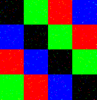
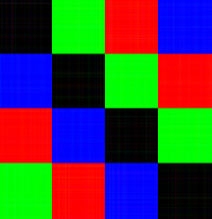
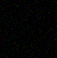
Figure 2: Low-rank approximations of color image. A noised color image ${\bf A}$ of size $200\times 200$ (left), the reconstruction by using $k$ largest singular triplets (middle), and the reconstruction by using $k$ smallest singular triplets (right).

5 Numerical Experiments

In this section, we compare our algorithms with five state-of-the-art algorithms by several numerical examples. These algorithms are listed as follows.

• irlba(R)–implicitly restarted Lanczos bidiagonalization method (Ritz vector) [1].

• irlba(H)—implicitly restarted Lanczos bidiagonalization method (harmonic vector) [1].

• irlbaMS(R)–implicitly restarted multi-symplectic Lanczos bidiagonalization method (Ritz vector) in Section 3.2.

• irlbaMS(H)–implicitly restarted multi-symplectic Lanczos bidiagonalization method (harmonic vector) in Section 3.3.

• lansvdQ–the Lanczos method for partial quaternion singular value [22].

• eigQ–the quaternion eigenvalue decomposition [19].

• svdQ–the quaternion singular value decomposition [30, 22].

All the experiments were performed in Matlab on a personal computer with 3.20 GHz Intel Core i5-3470 processor and 8 GB memory. According to equation (13), our numerical method outputs $\{\sigma_{j}^{(\mathcal{S})},\tilde{u}_{j}^{(\mathcal{S})},\tilde{v}_{j}^{(\mathcal{S})}\}$ as a singular triplet of $M^{(\mathcal{S})}$ if

$$\beta_{k}|(e_{k}^{(\mathcal{S})})^{T}u_{j}^{(\mathcal{S})}|\leq\delta\|M^{(\mathcal{S})}\|$$

for a user-specified value of $\delta$, where we have used $\beta_{k}=\|r_{k}^{(S)}\|$. The quantity $\|M^{(\mathcal{S})}\|$ is easily approximated by the singular value $\sigma_{1}^{(B_{k})}$ of largest magnitude of the bidiagonal matrix $B_{k}$. The computation of $\sigma_{1}$ is inexpensive because the matrix $B_{k}$ is small. The residuals are calculated by

$$\text{Residual}=\|M^{(\mathcal{S})}V_{k}^{(\mathcal{S})}-U_{k}^{(\mathcal{S})}\Sigma_{k}^{(\mathcal{S})}\|_{F},$$

where $U_{k}^{(\mathcal{S})},\Sigma_{k}^{(\mathcal{S})}$ and $V_{k}^{(\mathcal{S})}$ are formed by $k$ calculated singular triplets. The parameters are defined as follows:

Notation	Meaning	Default Value
$k$	Number of desired singular triplets	$10$
$maxit$	Maximum number of restarts	$2000$
$\delta$	Tolerance value	1.0E-10
$m_{b}$	Size of the Lanczos bidiagonal matrix $B_{k}$	$\max(2k,40)$

Example 5.1 (Sparse and JRS-Symmetric Matrix).

In this example, let the large-scale matrix $M^{(\mathcal{S})}\in\mathbb{R}^{4n\times 4n}$ be of the form (4) and let four sparse matrices $M^{(0)}$, $M^{(1)}$, $M^{(2)}$ and $M^{(3)}$ be the order-$n$ principle submatrices of bcspwr10, af23560, rw5151 and rdb5000 (from Matrix Market). Setting $n=3000$ and $m_{b}=40$, we compute the $k$ largest and smallest singular triplets of $M^{(\mathcal{S})}$ by algorithms irlba(R), irlba(H), irlbaMS(R) and irlbaMS(H). The CPU times and accuracies are listed in Table 1 and 2, respectively. The notation $n.c.$ means that the algorithm does not converge in $2000$ restarts.

From these numerical results, we can see that the multi-symplectic algorithms, irlbaMS(R) and irlbaMS(H), are fast and more accuracy than the standard methods, irlba(R) and irlba(H). Obviously, irlbaMS(H) performs better than irlbaMS(R) on computing the partial smallest singular triplets, while the later performs better on the calculating the partial largest singular triplets. In the case of computing the $k$ smallest singular triplets, both irlba(R) and irlba(H) do not converge after $2000$ restarts for $k=1$ and $5$, and need more than $1300$ restarts to converge when $k=10$. In Figure 3, we draw the convergence curves of the first $10$ singular triplets, i.e., $\beta_{k}|(e_{k}^{(S)})^{T}u_{j}^{(S)}|$. These convergence curves indicate that the multi-symplectic algorithms converge fast and stably, which indicate the advantages of the structure-preserving transformations.

Table 1: Calculating the first $k$ largest singular triplets

$k$	$Algorithm$	$Iter$	$CPU\ time$	$Residual$
	irlba(R)	1	2.0543	2.5685e-12
	irlba(H)	1	2.0722	1.6620e-12
$k=1$	irlbaMS(R)	2	0.5568	5.6299e-13
	irlbaMS(H)	2	0.6155	6.2253e-13
	irlba(R)	2	3.1450	2.6519e-12
	irlba(H)	2	3.1055	2.6195e-12
$k=5$	irlbaMS(R)	5	1.0656	2.4038e-12
	irlbaMS(H)	5	1.3251	2.8619e-12
	irlba(R)	3	4.5286	2.6184e-12
	irlba(H)	3	4.4223	2.4965e-12
$k=10$	irlbaMS(R)	8	1.6678	2.4815e-12
	irlbaMS(H)	8	1.7613	4.8367e-12
	irlba(R)	13	5.5461	1.5729e-08
	irlba(H)	12	5.6529	1.6638e-08
$k=20$	irlbaMS(R)	28	2.3643	7.9533e-12
	irlbaMS(H)	27	2.5107	1.3867e-11

Table 2: Calculating the first $k$ smallest singular triplets

$k$	$Algorithm$	$Iter$	$CPU\ time$	$Residual$
	irlba(R)	n.c.	-	-
	irlba(H)	n.c.	-	-
$k=1$	irlbaMS(R)	101	14.7813	6.9991e-12
	irlbaMS(H)	101	15.9442	2.7430e-12
	irlba(R)	n.c.	-	-
	irlba(H)	n.c.	-	-
$k=5$	irlbaMS(R)	56	8.4573	4.1946e-12
	irlbaMS(H)	57	8.7713	3.7882e-12
	irlba(R)	1867	2.2191e+03	2.7272e-02
	irlba(H)	1357	1.6563e+03	1.5109e-07
$k=10$	irlbaMS(R)	50	6.4715	8.1583e-12
	irlbaMS(H)	48	6.5680	3.5577e-12
	irlba(R)	814	2.9945e+02	1.1936e+01
	irlba(H)	929	3.5441e+02	6.3242e-05
$k=20$	irlbaMS(R)	154	10.6774	6.4510e-11
	irlbaMS(H)	145	11.3145	4.6488e-11

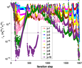
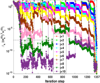
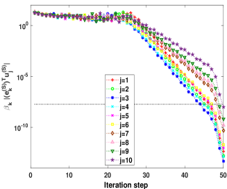
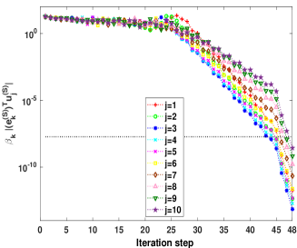
Figure 3: The convergence curves of the first $10$ largest singular triplets by irlba(R) (top left), irlba(H) (top right) , irlbaMS(R) (bottom left) and irlbaMS(H) (bottom right)

Example 5.2 (Dense Quaternion Matrices).

In this example, the quaternion matrix ${\bf A}\in\mathbb{Q}^{m\times n}$ is randomly generated as in [22]. The algorithms irlbaMS(R), irlbaMS(H), irlba(R), irlba(H), svdQ, and lansvdQ are applied to compute the $k$ largest or smallest singular triplets of ${\bf A}$. The parameters are set as follows. $m=2000,~{}n=200:200:2000$ and $m_{b}=40$.

In Figure 4, we compute the first $k$ ($=1$ or $10$) largest singular triplets of ${\bf A}$. In both cases, irlbaMS(R) and irlbaMS(H) are faster than irlba(R), irlba(H) and svdQ; lansvdQ is the fastest one. When $k=1$, all five algorithms have comparable residual norms; when $k$ increases, say $k=10$, the residues of lansvdQ are larger than those of other methods. In Figure 5, we compute the first $k$ ($=1$ or $10$) smallest singular triplets. irlbaMS(R) and irlbaMS(H) are indicated to be faster and more stable than irlba(R), irlba(H) and svdQ in general. We can conclude from Figure 4 and Figure 5 that the multi-symplectic methods, irlbaMS(R) and irlbaMS(H), perform better than the traditional methods, irlba(R) and irlba(H).

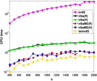
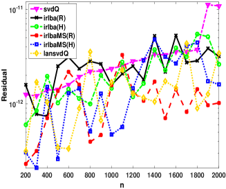
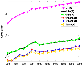
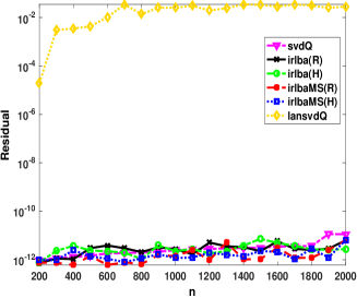
Figure 4: CPU times (left column) and residuals (right column) on calculating the first $k$ largest singular triplets. Parameters setting: $m_{b}=40$ and $k=1$(top row) or $10$ (bottom row).

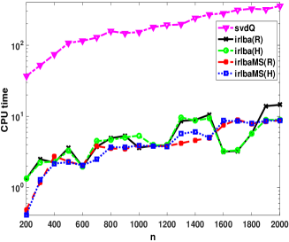
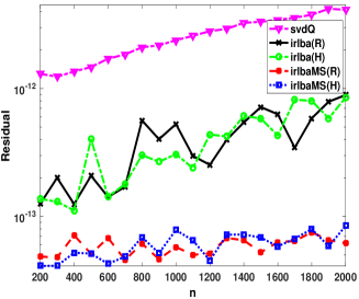
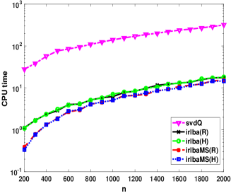
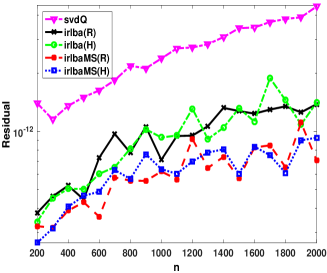
Figure 5: CPU times (left column) and residuals (right column) on calculating the first $k$ smallest singular triplets. Parameters setting: $m_{b}=40$ and $k=1$(top row) or $10$ (bottom row).

Example 5.3 (Color Face Recognition).

Color information is one of the most important characteristics in reflecting the structural information of an image. Face recognition performance with color images can be significantly better than that with grey-scale images; see, e.g., [18]. Suppose that there are $l$ training color image samples, denoted by $m\times n$ pure quaternion matrices ${\bf F}_{1},{\bf F}_{2},\ldots,{\bf F}_{l}$, and the average is $\Psi=\frac{1}{l}\sum_{s=1}^{l}{\bf F}_{s}\in\mathbb{Q}^{m\times m}$. Let

$${\bf X}=[vec({\bf F}_{1})-vec(\Psi),\cdots,vec({\bf F}_{l})-vec(\Psi)],$$

where $vec(\cdot)$ means to stack the columns of a matrix into a single long vector. The core work of color principal component analysis is to compute the right singular vectors corresponding to first $k$ largest singular values of ${\bf X}$. These vectors are called eigenfaces, and generate the projection subspace, denoted as ${\bf V}$.

In this experiment, we apply lansvdQ, eigQ and irlbaMS(R) into color images principal component analysis, based on the Georgia Tech face database. The setting is same to [22]. All images in the Georgia Tech face database are manually cropped, and then resized to $120\times 120$ pixels. There are $50$ persons to be used. The first ten face images per individual person are chosen for training and the remaining five face images are used for testing. The number of chosen eigenfaces, $k$, increases from 1 to 30. In each case, computing $k$ largest singular triplets of a quaternion matrix, ${\bf X}$, of size $14400\times 500$. Here the $14400$ rows refer to $120\times 120$ pixels and the $500$ columns refer to $50$ persons with $10$ faces each.

The detailed comparison on CPU times and recognition accuracies of these methods is shown in Figure 6. We see that irlbaMS(R) is faster than other the two algorithms, while the recognition accuracies are almost same.

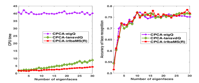
Figure 6: The CPU time and the accuracy by lansvdQ, eigQ and irlbaMS(R).

Example 5.4 (Color Video Compressing and Reconstruction).

All frames of a color video can be stacked into a quaternion matrix, ${\bf A}\in\mathbb{Q}^{(lm)\times n}$, where $l$ is the number of frames, and $m$ and $n$ denote numbers of rows and columns of each frame, respectively. Based on the SVD theory of quaternion matrix, the optimal rank-$k$ approximation to ${\bf A}$ can be reconstructed from its first $k$ largest singular values and corresponding left/right singular vectors. Denote such approximation as

$${\bf A}_{k}={\bf U}_{k}S_{k}{\bf V}_{k}^{*},$$

where $S_{k}=\texttt{diag}(\sigma_{1},\ldots,\sigma_{k})$ consists of the first $k$ largest singular values of ${\bf A}$, and the columns of ${\bf U}_{k}$ and ${\bf V}_{k}$ are left and right corresponding singular vectors. Then the relative distances from ${\bf A}_{k}$ to ${\bf A}$ are

$$\frac{\|{\bf A}_{k}-{\bf A}\|_{2}}{\|{\bf A}\|_{2}}=\frac{\sigma_{k+1}}{\|{\bf A}\|_{2}},\ \ \frac{\|{\bf A}_{k}-{\bf A}\|_{F}}{\|{\bf A}\|_{F}}=\frac{(\sum_{j=k+1}^{min(lm,n)}\sigma_{j}^{2})^{\frac{1}{2}}}{\|{\bf A}\|_{F}}.$$ (51)

In this example, we apply lansvdQ, eigQ and irlbaMS(R) to compute $k$ largest quaternion singular triplets of a large-scale video quaternion matrix. The direct method eigQ is firstly used to compute the eigenvalue problem of the Hermitian quaternion matrix ${\bf A}^{*}{\bf A}$. The eigenvectors of ${\bf A}^{*}{\bf A}$ are in fact the left singular vectors of ${\bf A}$, saved in a unitary matrix ${\bf V}$, and the square roots of the eigenvalues are the singular values, saved in a diagonal matrix $S$. The right singular vectors of ${\bf A}$ is generated by ${\bf U}={\bf A}{\bf V}S^{-1}$. Let $\hat{{\bf U}}_{k}={\bf U}(:,1:k)$, $\hat{S}_{k}=S(1:k,1:k)$, and $\hat{{\bf V}}_{k}={\bf V}(:,1:k)$, then we get another approximation to ${\bf A}$, $\hat{{\bf A}}_{k}=\hat{{\bf U}}_{k}\hat{S}_{k}\hat{{\bf V}}_{k}$. We expect that these methods can achieve at the same accuracy, but the costed CPU time of irlbaMS(R) is shortest.

Let ${\bf F}$ and ${\bf F}_{k}$ denote the original frame and its approximation, respectively. The peak signal-to-noise ratio (PSNR) value of $F_{k}$ is defined as

$$PSNR(F_{k},F)=10*log_{10}(\frac{255^{2}mn}{\|F_{k}-F\|_{F}^{2}})$$

The structural similarity (SSIM) index of $F_{k}$ and F is defined as

$$SSIM(F_{k},F)=\frac{(4\mu_{x}\mu_{y}+c_{1})(2\sigma_{xy}+c_{2})}{(\mu_{x}^{2}+\mu_{y}^{2}+c_{1})(\sigma_{x}^{2}+\sigma_{y}^{2}+c_{2})},$$

where $x$ and $y$ denote the vector forms of $F$ and $F_{k}$, respectively, $\mu_{x,y}$ denotes the average of $x$, $y$, $\sigma_{x,y}$ the variance of $x$, $y$, $\sigma_{xy}$ the covariance of $x$ and $y$, and $c_{1,2}$ are two constants.

First, we take the color video $yunlonglake.mp4$ provided in [22] for testing the efficiencies of lansvdQ, eigQ and irlbaMS(R) on color video compressing and reconstruction. This video consists of 31 frames (each frame is of size 544$\times$960). Second, we test two methods with the color video, children.mov(from [22]), which consists of 20 frames and each frame is of size 1280$\times$360. The relative distances defined as in (51), PSNR and SSIM values of the approximations to randomly chosen 10 frames by three methods are computed and the average values are shown in Table 3. The CPU times of computing $k$ singular triplets by lansvdQ, eigQ and irlbaMS(R) are shown in Figure 7. We can see that irlbaMS(R) is the fastest one.

Table 3: The average relative distances, PSNR and SSIM values of the approximations of 10 frames with applying $k$ singular triplets ($k=30$).

Video	Method	PSNR	SSIM	$\frac{\|A_{k}-A\|_{2}}{\|A\|_{2}}$	$\frac{\|A_{k}-A\|_{F}}{\|A\|_{F}}$
	eigQ	29.5953	0.9236	0.0148	0.0620
yunlonglake	lansvdQ	29.5953	0.9236	0.0148	0.0620
	irlbaMS(R)	29.5953	0.9236	0.0148	0.0620
	eigQ	23.4508	0.8428	0.0273	0.1243
children	lansvdQ	23.4508	0.8428	0.0273	0.1243
	irlbaMS(R)	23.4508	0.8428	0.0273	0.1243

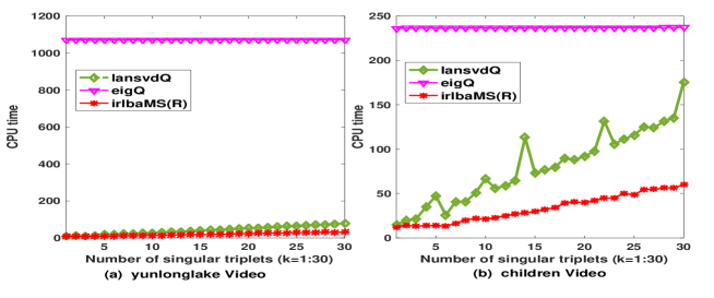
Figure 7: The computational CPU times of $k$ singular triplets by lansvdQ, eigQ and irlbaMS(R). x-axis: the number of singular triplets; y-axis: CPU times.

6 Conclusion

In this paper, a multi-symplectic Lanzcos method is proposed and applied to compute the $k$ largest and smallest singular triplets of JRS-symmetric matrix. The augmented Ritz and harmonic Ritz vector are applied respectively to perform implicitly restarting to obtain a satisfactory bidiagonal matrix. Two new associated algorithms are presented: irlbaMS(R) and irlbaMS(H). irlbaMS(H) is the first reliable algorithm of computing $k$ smallest singular triplets to the best of our knowledge. The proposed multi-symplectic algorithms performs better than the state-of-the-art algorithms in numerical experiments.

References

- [1] Baglama, J. and Reichel, L.: Augmented implicitly restarted Lanczos bidiagonalization methods. SIAM J. Sci. Comput. 27(1), 19-42, 2005.
- [2] Beattie C. A., Mehrmann V., and Van Dooren P.: Robust port-Hamiltonian representations of passive systems. Automatica 100, 182-186, 2019.
- [3] Benner P.: Symplectic balancing of Hamiltonian matrices. SIAM J. Sci. Comput. 22(5), 1885-1904, 2001.
- [4] Benner P., Byers R., Mehrmann V., and Xu H.: Numerical computation of deflating subspaces of skew-Hamiltonian/Hamiltonian pencils. SIAM J. Matrix Anal. Appl. 24(1), 165-190, 2002.
- [5] Benner, P., Fabender, H., and Stoll, M.: A Hamiltonian Krylov-Schur-type method based on the symplectic Lanczos process. Linear Algebra Appl. 435, 578-600, 2011.
- [6] Björck, A., Grimme, E., and Van Dooren, P.: An implicit bidiagonalization algorithm for ill-posed systems. BIT 34, 510-534, 1994.
- [7] Björck, A.: Numerical Methods for Least Squares Problems. SIAM, Philadelphia, 1996.
- [8] Bunch, J.R. and Nielsen, C.P.: Updating the singular decomposition. Numer. Math. 31, 111-129,1978.
- [9] Chan, R.H. and Ng, M.K.: Conjugate gradient methods for Toeplitz systems. SIAM Review. 38(3), 427-482, 1996.
- [10] R. Chan and X. Jin: An Introduction to Iterative Toeplitz Solvers, SIAM, Philadelphia, 2007.
- [11] Demmel, J.W.: Applied Numerical Linear Algebra. SIAM, Philadelphia, 1997.
- [12] Fukunaga, K.: Introduction to Statistical Pattern Recognition, 2nd ed. Academic Press, San Diego, CA, 1991.
- [13] Golub, G.H. and Kahan, W.: Calculating the singular values and pseudo-inverse of a matrix. J. Soc. Indust. Appl. Math. Ser. B Numer. Anal. 2, 205-224, 1965.
- [14] Golub, G.H. and Van Loan, C.F.: Matrix Computation, 4th edn. The Johns Hopkins University Press, Baltimore, 2013.
- [15] Gu, M. and Eisenstat, S.C.: A stable and fast algorithm for updating the singular value decomposition. Technical report YALEU/DCS/RR-966, Department of Computer Science, Yale University, New Haven, CT, 1993.
- [16] Hamilton, W.R.: Elements of Quaternions. Chelsea, New York, 1969.
- [17] He, X. and Niyogi, P.: Locality preserving projections, in Proceedings of the Conference on Advances in Neural Information Processing Systems, pp. 153-160, 2003.
- [18] Jia, Z.G., Ling, S., and Zhao, M.: Color two-dimensional principal component analysis for face recognition based on quaternion model. LNCS 10361, ICIC (1): 177-189, 2017.
- [19] Jia, Z.G., Wei, M., and Ling, S.: A new structure-preserving method for quaternion hermitian eigenvalue problems. J. Comput. Appl Math. 239, 12-24, 2013.
- [20] Jia, Z.G., Wei, M., Zhao, and M., Chen, Y.: A new real structure-preserving quaternion QR algorithm. J. Comput. Appl. Math. 343, 26-48, 2018.
- [21] Jia Z.G., Ng M.K., and Song G.J.: Robust quaternion matrix completion with applications to image inpainting, Numer. Linear Algebra Appl., 26(4), e2245, 2019.
- [22] Jia Z.G., Ng M.K., and Song G.J.: Lanczos method for large-scale quaternion singular value decomposition, Numer. Algorithms, 82(2), 699-717, 2019.
- [23] Jia Z.G., Ng M.K., and Wang W.: Color image restoration by saturation-value (SV) total variation, SIAM J. Imaging Sciences, 12(2), 972-1000, 2019.
- [24] Jia, Z. and Niu, D.: An implicitly restarted refined bidiagonalization Lanczos method for computing a partial singular value decomposition. SIAM J. Matrix Anal. Appl. 25, 246-265, 2003.
- [25] Jin X.: Preconditioning Techniques for Toeplitz Systems, Higher Education Press, Beijing, 2010.
- [26] Ke R., Ng M., and Sun H.: A fast direct method for block triangular Toeplitz-like with tri-diagonal block systems from time-fractional partial differential equations, J. Comput. Phys., 303, 203-211, 2015.
- [27] Kokiopoulou, E., Bekas, C., and Gallopoulos, E.: Computing smallest singular triplets with implicitly restarted Lanczos bidiagonalization. Appl. Numer. Math., 49, 39-61, 2004.
- [28] Kokiopoulou, E., and Saad, Y.: Enhanced graph-based dimensionality reduction with repulsion Laplaceans. Pattern Recogn. 42, 2392-2402, 2009.
- [29] Kokiopoulou, E., and Saad, Y.: Orthogonal neighbourhood preserving projections. in Proceedings of the 5th International IEEE Conference on Data Mining, Houston, TX, IEEE, 234-241, 2005.
- [30] Li Y., Wei M., Zhang F. X., and Zhao J. L.: A fast structure-preserving method for computing the singular value decomposition of quaternion matrix. Appl. Math. Comput., 235, 157-167, 2014.
- [31] Li Y., Wei M., Zhang F. X., and Zhao J. L.: Real structure-preserving algorithms of Householder based transformations for quaternion matrices. J. Comput. Appl. Math., 305, 82-91, 2016.
- [32] Ling, S., Jia, Z., Lu, X., and Yang, B., Matrix LSQR algorithm for structured solutions to quaternionic least squares problem. Comput. Appl. Math., 77(3), 830-845, 2019.
- [33] Ma, R., Jia, Z., and Bai, Z.: A structure-preserving Jacobi algorithm for quaternion Hermitian eigenvalue problems. Comput. Appl. Math. 75(3), 809-820, 2018.
- [34] Mehl C., Mehrmann V., and Sharma P.: Stability radii for linear Hamiltonian systems with dissipation under structure-preserving perturbations. SIAM J. Matrix Anal. Appl. 37(4), 1625-1654, 2016.
- [35] Mehl C., Mehrmann V., and Wojtylak M.: Linear algebra properties of dissipative Hamiltonian descriptor systems. SIAM J. Matrix Anal. Appl. 39(3), 1489-1519, 2018.
- [36] Morgan, R.B.: Computing interior eigenvalues of large matrices. Linear Algebra Appl. 154/156, pp. 289-309, 1991.
- [37] Ng, M.K.: Iterative Methods For Toeplitz Systems. Oxford University Press, USA, 2004.
- [38] Ngo, T.T., Bellalij, M., and Saad, Y.: The trace ratio optimization problem. SIAM Review 54:3, 545-569, 2012.
- [39] Paige, C.C., Parlett, B.N., and van der Vorst, H.A.: Approximate solutions and eigenvalue bounds from Krylov subspaces. Numer. Linear Algebra Appl. 2(2), 115-134, 1995.
- [40] Pei, S.C. and Cheng, C.M.: A novel block truncation coding of color images by using quaternion-moment-preserving principle, IEEE International Symposium on Circuits and Systems. 45(5), 583-595, 1997.
- [41] Roweis, S. and Saul, L.: Nonlinear dimensionality reduction by locally linear embedding, Science. 290, pp. 2323-2326, 2000.
- [42] Sangwine, S.J.: Fourier transforms of colour images using quaternion or hypercomplex numbers. Electron. Lett. 32(1), 1979-1980, 1996.
- [43] Simon, H.D. and Zha, H.: Low-rank matrix approximation using the Lanczos bidiagonalization process with applications. SIAM J. Sci Comput. 21(6), 2257-2274, 2000.
- [44] Sorensen, D.C.: Implicit application of polynomial filters in a -Step arnoldi method. SIAM J. Matrix Anal. Appl., 13, 357-385, 1992.
- [45] Wei M., Li Y., Zhang F. X., and Zhao J. L.: Quaternion Matrix Computations, Nova Science Publishers, 2018.
- [46] Zhang, F.: Quaternions and matrices of quaternions. Linear Algebra Appl. 251, 21-57, 1997.