The range of Jupiter’s flow structures that fit the Juno asymmetric gravity measurements

Abstract

The asymmetric gravity field measured by the Juno spacecraft has allowed the estimation of the depth of Jupiter’s zonal jets, showing that the winds extend approximately $3000$ km beneath the cloud level. This estimate was based on an analysis using a combination of all measured odd gravity harmonics, $J_{3}$, $J_{5}$, $J_{7}$, and $J_{9}$, but the wind profile’s dependence on each of them separately has yet to be investigated. Furthermore, these calculations assumed the meridional profile of the cloud-level wind extends to depth. However, it is possible that the interior jet profile varies somewhat from that of the cloud level. Here we analyze in detail the possible meridional and vertical structure of Jupiter’s deep jet-streams that can match the gravity measurements. We find that each odd gravity harmonic constrains the flow at a different depth, with $J_{3}$ the most dominant at depths below $3000$ km, $J_{5}$ the most restrictive overall, whereas $J_{9}$ does not add any constraint on the flow if the other odd harmonics are considered. Interior flow profiles constructed from perturbations to the cloud-level winds allow a more extensive range of vertical wind profiles, yet when the meridional profiles differ substantially from the cloud level, the ability to match the gravity data significantly diminishes. Overall, we find that while interior wind profiles that do not resemble the cloud level are possible, they are statistically unlikely. Finally, inspired by the Juno microwave radiometer measurements, assuming the brightness temperature is dominated by the ammonia abundance, we find that depth-dependent flow profiles are still compatible with the gravity measurements.

¹Department of Earth and Planetary Sciences, Weizmann Institute of Science, Rehovot, Israel.

Plain Language Summary

Jupiter’s north-south asymmetric gravity field, as measured by the Juno spacecraft, currently orbiting Jupiter, has been used to set the depth of its jet-streams (associated with the famous visible cloud bands) at approximately $\sim 3000$ km. This estimate was based on all the gravity field measurements combined. However, there is also information about the structure of the flow hidden in each individual measurement. Here we analyze these measurements and show how each of them constrains the flow at a different depth. We also systematically investigate the statistical likelihood of wind profiles that differ from the profile observed at the cloud level with various structures at depth. We find that Jupiter’s measured cloud-level jet streams fit with its gravity data only for a relatively narrow envelope of vertical structures. Although other jet profiles that are different from the one observed at the cloud level are feasible (still consistent with the gravity data), they are statistically unlikely. Finally, we explore a depth-dependent wind structure inspired by the Juno microwave radiometer instrument, which indicates that ammonia abundance varies with depth and might be correlated with the jet-streams. We find that such a profile can still match the gravity data as long as the variation from the cloud-level wind is not substantial.

1 Introduction

The Juno spacecraft has provided an unprecedented glance into Jupiter’s atmospheric flows below the cloud level. The high-precision gravity measurements, particularly those of the odd gravitational harmonics repeated in multiple passes (Iess et al.,, 2018), have presented an opportunity to estimate the depth and structure of Jupiter’s zonal jets. It has been found that the zonal jets are deep and penetrate to approximately $3000$ km below the cloud level (Kaspi et al.,, 2018). Below this depth, the even gravitational harmonics indicate that Jupiter rotates almost like a solid body (Guillot et al.,, 2018). However, determining the details of the decay profile with depth poses a significant challenge. Remnants of the zonal flows appear even below $4000$ km, and since the estimation of the electrical conductivity in Jupiter at this depth is at least $10\;{\rm S~{}m^{-1}}$ (Nellis et al.,, 1996; Wicht et al., 2019a, ; Wicht et al., 2019b, ), an interaction between the flow and the magnetic field is expected there (Cao and Stevenson,, 2017; Galanti et al., 2017a, ; Duer et al.,, 2019; Moore et al.,, 2019). Understanding the gravity harmonic signature and the flow structure below the cloud level is thus essential in order to build a better picture of Jupiter’s atmosphere.

The gravity field of Jupiter, represented by the gravity harmonics, reflects both the internal density structure and the deep zonal flow structure (Hubbard,, 1999; Kaspi et al.,, 2010). The even gravity harmonics are used to constrain the internal density structures of Jupiter and other gas giants (e.g., Hubbard et al.,, 1974, 1975; Helled et al.,, 2010; Nettelmann et al.,, 2013). Multiple studies have shown that the higher-order (even) gravity harmonics are sensitive to the outer regions of the planet (e.g., Zharkov and Trubitsyn,, 1974; Guillot and Gautier,, 2007; Nettelmann et al.,, 2013). Their exact value is defined by the density distribution throughout the planet and the planet’s rotation, composition, shape, mass, and radius. Since for a static gas planet, the odd harmonics are identically zero, any gravitational asymmetry between north and south would indicate a dynamical source generating those asymmetries (Kaspi,, 2013). Juno measured with high precision the gravity harmonics up to $J_{10}$, including significant odd values. The measured values and error range are: $J_{3}=\left(-4.24\pm 0.91\right)\times 10^{-8}$, $J_{5}=\left(-6.89\pm 0.81\right)\times 10^{-8}$, $J_{7}=\left(12.39\pm 1.68\right)\times 10^{-8}$ and $J_{9}=\left(-10.58\pm 4.35\right)\times 10^{-8}$ (Iess et al.,, 2018). The relation between the density anomaly and the flow (thermal wind balance) allows constraining the deep flow structure within the planet (Kaspi et al.,, 2010; Kaspi,, 2013; Kaspi et al.,, 2018). Assuming that the cloud-level zonal wind profile is extended towards Jupiter’s interior using a scaling factor, one can find many solutions for the deep flow structure that satisfy all four odd gravity harmonics within the uncertainty range. With the currently available data, Jupiter’s deep flow cannot be determined uniquely (Kaspi et al.,, 2018; Kong et al.,, 2018), and systematic exploration of the range of the deep flow structure is necessary.

Moreover, the meridional profile of the zonal wind is not necessarily constant with depth. The cloud-level wind itself has a measurement error (Garcıa-Melendo and Sánchez-Lavega,, 2001; Salyk et al.,, 2006; Tollefson et al.,, 2017), and as it extends inward, the profile might vary, although any such variation must be accompanied with a meridional temperature gradient as well. Some evidence for such meridional variations come from the Juno microwave radiometer (MWR) measurements showing that the nadir brightness temperature profile (dominated by the ammonia abundance) becomes smoother with depth (Bolton et al.,, 2017; Li et al.,, 2017). Although this measurement does not necessarily correlate with temperature, it does coincide, to some degree, with the zonal wind profile at the cloud level (Bolton et al.,, 2017), and thus might hint to the vertical variation of the zonal wind profile in the upper 300 km.

Previous work on constraining the deep flow structure was done using all four measured gravity harmonics combined (e.g., Kaspi et al.,, 2018; Kong et al.,, 2018). However, an important question is how does each gravity harmonic individually constrain the flow strength at different depths. Here, we examine the individual contribution of each odd gravity harmonic, with emphasis on the depth of influence and the relation to the cloud-level zonal wind profile. In order to provide a systematic analysis, we take a hierarchal approach, in which we increase the level of complexity of the variation of the wind structure, and in all cases explore what is the range of solutions that match the gravity measurements. We begin with solutions that are identical to the cloud-level profile and allow only for the vertical decay to vary. Then, we relax the constraint on the meridional profile of the zonal wind and allow variations from the measured cloud-level profile along with the varying vertical decay. Finally, we examine random meridional profiles that are not related at all to Jupiter’s measured cloud-level profile and explore the possibility that the interior wind structure, which influences the gravity measurements, is completely different from the cloud-level flow. Following this logic, we also search for solutions with smoother wind profiles that resemble the MWR measurements at 300 km (channel 1), and calculate the vertical profile of such flows that can match also the gravity data.

The paper is organized as follows: In section 2, we introduce the theoretical background for this analysis, connecting the gravity measurements and the wind profile. In section 3, we present the possible solutions for Jupiter’s wind profile, the depth sensitivity obtained by excluding a specific harmonic, and the contribution function of each harmonic. In section 4, we discuss the ability to find solutions for the anomalous gravity field of different meridional profiles, and in section 5, we explore depth-dependent meridional structures, inspired by the MWR measurements. We discuss the dynamical implications of the results and conclude in section 6.

2 Methodology

The density distribution within Jupiter is reflected in the zonal gravity harmonics $\left(J_{n}\right)$, which describe the external gravitational field of the planet in equilibrium (Zharkov and Trubitsyn,, 1974). The gravity harmonics can be represented by

$$J_{n} = -\frac{1}{MR_{J}^{n}}\int\rho r^{n}P_{n}\left(\mu\right)d^{3}r,$$ (1)

where $M$ and $R_{J}$ are Jupiter’s mass and equatorial radius, respectively, $n$ is the harmonic degree ($n=2,...,N$), $\rho$ is the density, $r$ is the radial coordinate and $P_{n}\left(\mu\right)$ is the $n$-th Legendre polynomial, where $\mu=\sin\theta$ and $\theta$ is the latitude (Hubbard,, 1984). The density can be decomposed such that $\rho\left(r,\theta\right)=\widetilde{\rho}\left(r,\theta\right)+\rho^{\prime}\left(r,\theta\right)$, where $\widetilde{\rho}\left(r,\theta\right)$ is the static component that is determined by the planet’s shape and rotation (Hubbard,, 2012), and $\rho^{\prime}\left(r,\theta\right)$ is the dynamical anomaly representing fluid velocities with respect to the solid body rotation (Kaspi et al.,, 2010). The zonal gravity harmonics that represent only the dynamical part of the flow $\left(\Delta J_{n}\right)$ can be calculated by integrating the density anomaly and its projection onto the Legendre polynomials in spherical coordinates such that

$$\Delta J_{n} = -\frac{2\pi}{MR_{J}^{n}}\intop_{0}^{R_{J}}\intop_{-1}^{1}\rho^{\prime}\left(r,\mu\right)r^{n+2}P_{n}\left(\mu\right)d\mu dr.$$ (2)

Since an oblate planet with no dynamics is symmetric between north and south, the density anomaly represented by the odd harmonics ($n=3,5,..$) should be identically zero if the flow pattern is symmetric, and will be very small if the dynamics are shallow ($\Delta J_{n}=J_{n}$ for odd $n$). However, Juno measured four odd gravity harmonics (Iess et al.,, 2018), indicating the existence of a strong asymmetric pattern in Jupiter’s flow field due to the existence of strong, deep winds.

The rapid rotation and size of the planet (small Rossby number) imply that this asymmetry is directly related to zonal flows, since, to first order, the leading balance in Jupiter is a geostrophic balance between the flow-related Coriolis forces and the pressure gradients. This leads to a vorticity balance known as thermal wind balance (Pedlosky,, 1987; Kaspi et al.,, 2009). If only zonal (azimuthal) flows are considered, the thermal wind balance can be written as

$$2\Omega r\frac{\partial\left(\tilde{\rho}u\right)}{\partial z} = g_{0}\frac{\partial\rho^{\prime}}{\partial\theta},$$ (3)

where $\Omega$ is Jupiter’s rotation rate, $u\left(r,\theta\right)$ is the zonal flow, $g_{0}\left(r\right)$ is the mean gravitational acceleration and $z$ is the direction parallel to the rotation axis. An equivalent equation can be written with temperature instead of density gradients, and one can easily switch between the two versions through the equation of state. Note that the barotropic limit of Eq. 3 is not simply when the rhs vanishes, but when $\frac{\partial u}{\partial z}=0$ (see full derivation at Kaspi et al., (2016)). Galanti et al., 2017b showed that a higher order expansion, beyond thermal wind, only slightly adjusts the deep flow dynamics (less than $10\%$). Therefore, for the purpose of studying the overall vertical profile, Eq. 3 is a good approximation.

Our goal here is to search for possible deep wind structures that can explain each of the measured odd gravity harmonics ($J_{3,\>}J_{5,\>}J_{7,}$ and $J_{9}$). Unlike previous studies (e.g., Kaspi et al.,, 2018), we are not solving for an optimal solution with respect to the full error covariance matrix. Any vertical wind profile that fits the odd measured gravity harmonics, within the uncertainty range of Juno, is considered a possible solution for the flow. This allows us to examine the full range of possible solutions, without converging on a single decay profile of the flow. For example, the optimal solution suggested by Kaspi et al., (2018) that considered the error covariance matrix is not a solution here since the value of $J_{3}$ is not within the measured error.

3 The vertical profile of the zonal flow

Taking a hierarchal approach entailing an increasing level of complexity, we first use the observed cloud-level wind as an upper boundary condition for the flow field and assume the same profile continues inward in a direction parallel to the spin axis, due to angular momentum considerations (Busse,, 1976; Kaspi et al.,, 2010). The possible deep flow structures are then set to decay continuously from the cloud level to a few thousand kilometers below it (Kaspi et al.,, 2018), using two different decay regions. Dividing the decay functions into two distinct regions stems from the magnetic field’s possible effects on the flow, expected approximately at $r<0.97\,R_{J}$ (Duer et al.,, 2019; Wicht et al., 2019a, ), which imply that once the electrical conductivity becomes dominant, the magnetic field acts to dissipate the flow (Liu et al.,, 2008; Gastine et al.,, 2014). Thus, for the lower part (the semiconducting region), we chose an exponential decay (Eq. 6, $r<R_{T}$) that fits the exponential nature of the electrical conductivity within Jupiter (Nellis et al.,, 1992; Weir et al.,, 1996; French et al.,, 2012). For the upper part, the vertical decay function includes both an exponent and hyperbolic tangent (Eq. 5, $R_{T}\leq r\leq R_{J}$), which combine to give a wide range of possible decay profiles.

The vertical profile of the zonal flow is defined with six independent parameters, chosen to cover an extensive range of vertical profiles. It is set as

$$u(\theta,r)=u_{{\rm proj}}(\theta,r)Q_{s}(r),$$ (4)

$$Q_{s}(r)=(1-\alpha)\exp\left(\frac{r-R_{J}}{H_{1}}\right)+\alpha\left[\frac{{\rm tanh}\left(-\frac{R_{J}-H_{2}-r}{\Delta H}\right)+1}{{\rm tanh}\left(\frac{H_{2}}{\Delta H}\right)+1}\right]\qquad R_{T}\leq r\leq R_{J},$$ (5)

$$Q_{s}(r)={Q_{s}(R_{T})}\exp\left(\frac{r-R_{T}}{H_{3}}\right)\qquad r<R_{T},$$ (6)

where $u_{{\rm proj}}(r,\theta)$ is the wind at the cloud level, projected inwards (with no decay) in the direction parallel to the axis of rotation ($\hat{z}$-axis, Eq. 3), $Q_{s}(r)$ is the radial decay function, representing the fraction of the cloud-level wind at every depth, and the set of parameters that forms the decay are bounded by the following limits: $0\leq\alpha\leq 1$, $200$ km $\leq H_{1}\leq 2500$ km, $200$ km $\leq H_{2}\leq 2500$ km, $200$ km $\leq\Delta H\leq 2500$ km, $0.95\leq R_{T}\leq 0.975\,R_{J}$ and $100\leq H_{3}\leq 900$ km. The function $Q_{s}$ is also smoothed at the transition depth. We vary the parameters uniformly between their lower and upper bounds, taking only profiles where the wind speed decays monotonically as viable options. In total, we consider $5\times 10^{5}$ decay profiles, sufficiently covering the parameter space. This set of decay profiles serves as the sample population for this study. For each profile, we calculate the associated density anomaly and the implied odd gravity harmonics. All the calculations presented below are performed using the same sample population. Note that other forms of $Q_{s}$ are possible, and can still fit the measured gravity data ($Q_{s}(r,\theta)$, for example, as explored in Kaspi et al., (2018)). However, we have found that for the exploration of the individual gravity harmonic depth sensitivities and the meridional profile anomalies, the chosen function, which allows a very wide range of decay profiles, is satisfactory.

From the $5\times 10^{5}$ decay options examined, $6712$ vertical profiles are compatible with Juno’s measured odd gravity harmonics, which represent a little over $1\%$ of the sample population (Fig. 1a). All the compatible decay profiles are located in a relatively narrow envelope, especially in the region around $2000$ km depth and the one below $4000$ km, with all the options pointing to remnants of jet-associated velocities at a depth of $4000$ km (Fig. 1). Those deep velocities are still on the order of $1$ ${\rm m~{}s^{-1}}$ and despite being small, they are still higher than the magnetic secular variation associated velocities estimated by Moore et al., (2019). Increasing the error range of Juno’s gravity measurements does allow for more solutions, but the overall structure does not change much (Fig. 1b).

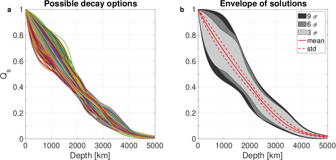
Figure 1: (a) Decay options that fit all four measured odd gravity harmonics $\left(J_{n}\right)$ within the $3\sigma$ sensitivity range of Juno, using Jupiter’s observed cloud-level flows (Tollefson et al.,, 2017). (b) Envelope of all possible solutions (light gray), the average solution of all options (red line), their standard deviation (dashed red lines) and envelope of solutions satisfying larger uncertainty range (darker gray with rising uncertainty range).

3.1 The depth sensitivity of the odd harmonics

Research to date has focused on finding vertical profiles that match all four odd gravity harmonics. However, there is information to be obtained from each gravity harmonic separately. Here, vertical flow profiles that fit three out of the four measured odd gravity harmonics are considered, and the depth sensitivity of the excluded harmonic is studied by examining the difference between the vertical profiles that include the specific $J_{n}$ to those that do not necessarily include it. The resulting depth sensitivity of each odd measured gravity harmonic, according to Jupiter’s measured zonal profile, is presented in Fig. 2. The gray envelope, the same one as in Fig. 1b, is the boundary of all the possible solutions that fit all four odd gravity harmonics within $3\sigma$. Note that not all possible profiles inside the gray envelope will necessarily generate a solution compatible with the measured gravity field, since the solution is also dependent on the decay profile within the given envelope. All the other solutions gained while excluding one of the odd gravity harmonics appear in Fig. 2 (turquoise envelopes). The turquoise envelopes always contain the gray envelopes by definition, since they are constructed by fitting at least three gravity harmonics. The difference between the turquoise envelopes and the gray ones denote the region in which the excluded harmonic bounds the flow.

The most insignificant influence is clearly of $J_{9}$ (Fig. 2d). It appears to add no solutions at all to the gray envelope, meaning that $J_{9}$ does not constrain the flow if the other three odd values are still within Juno’s $3\sigma$. This is likely because $J_{9}$ has the highest measurement error and lowest signal-to-noise ratio (SNR), so even while fitting $J_{9}$, there is an extensive region of solutions, and excluding it does not add new solutions. The largest influence on the flow profile and depth sensitivity comes from $J_{5}$ (Fig. 2b). It appears to set the upper boundary of the gray envelope from the cloud level ($0$ km) to $3500$ km, and a lower boundary of the gray envelope between $2000$ to $3500$ km. The strongest sensitivity is between the cloud level and $3000$ km. $J_{5}$ has the smallest measured $3\sigma$ value and largest SNR, but its value is very similar to the SNR of $J_{7}$, so the large influence of $J_{5}$ cannot be a result of the SNR alone. In a similar manner, $J_{3}$ is mostly sensitive between $3000$ and $5000$ km and between the cloud level ($0$ km) and $1500$ km (Fig. 2a). Note that a flow profile that decays to zero at $4000$ km ($\sim 0.94\,R_{J}$) cannot fit $J_{3}$. $J_{7}$ is sensitive between $500$ and $2500$ km, and sets mainly the lower boundary of the gray envelope at those depths (Fig. 2c).

Previous studies that examined the depth dependency of the even gravity harmonics (resulting from the shape and density of a solid-body model, without differential flows) concluded that higher-order harmonics are more sensitive to the density in the outer regions (e.g., Zharkov and Trubitsyn,, 1974; Guillot and Gautier,, 2007; Nettelmann et al.,, 2013). This is implied by the radial dependence of the gravity harmonics (Eq. 1). However, the above analysis shows that the wind-induced odd harmonics’ depth dependency is more complicated. One exception is $J_{3}$, the only harmonic that is sensitive below $4000$ km, which resembles the even harmonics’ depth tendency, where the low-order harmonics are more sensitive in deeper regions.

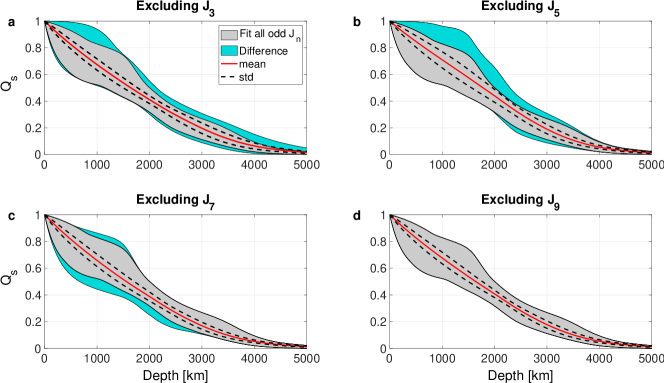
Figure 2: (a) The envelope of possible solutions that fit all four odd gravity harmonics (gray), the envelope of additional solutions once excluding $J_{3}$ (while still fitting $J_{5}$, $J_{7}$ and $J_{9}$) (turquoise), the average of all decay options within the panel (gray and turquoise combined) (red), and their standard deviation (dashed black). The other panels are the same while excluding other $J_{n}$: (b) excluding $J_{5}$, (c) excluding $J_{7}$ and (d) excluding $J_{9}$. The results are a combination of the sample decay options ($5\times 10^{5}$). Note that the turquoise color emphasizes the depth sensitivity of each gravity harmonic separately.

3.2 The contribution function

The depth sensitivity of the gravity harmonics can also be examined by calculating directly the depth dependence of $J_{n}$, defined as the contribution function. This function was calculated in past studies for the even harmonics of Jupiter and other planets (e.g., Guillot and Gautier,, 2007; Helled et al.,, 2010; Nettelmann et al.,, 2013). The contribution of each shell is the normalized integrant of $J_{n}$, defined as

$$C_{n}=\frac{1}{J_{n}}\frac{dJ_{n}}{dr}=\frac{1}{J_{n}}\frac{-2\pi}{MR_{J}^{n}}\intop_{-1}^{1}\rho\left(r,\mu\right)r^{n+2}P_{n}\left(\mu\right)d\mu$$ (7)

(Zharkov and Trubitsyn,, 1974; Hubbard et al.,, 1974; Hubbard,, 1984). The even harmonics in past studies were calculated from the background density (solid body models), while in our study we use the wind-induced anomalous density field to calculate the odd harmonics’ contribution, taking $\rho^{\prime}$ instead of $\rho$ in Eq. 7.

The averaged anomalous density profile of all possible decay structures, that are consistent with the four odd gravity harmonics, is presented in Fig. 3a. The anomalous density reveals a change of sign at $2000$ km. The averaged odd contribution functions ($C_{n}$) and standard deviations of each odd gravity harmonic (Fig. 3b) corresponding to the solution envelope from Fig. 1 show a consistent sign change. Note that the change of sign is exhibited only by the anomalous density, corresponding to the wind shear with depth, and, therefore, does not exist when examining the even harmonics resulting from the static density (e.g., Nettelmann et al.,, 2013). The integrals of the non-normalized contribution curve, $C_{n}$, are the gravity harmonic values, $J_{n}$, so the sign and value of $J_{n}$ are set by the difference between the positive and negative curves (above and below $2000$ km, not shown). For the averaged anomalous density, the gravity harmonics are: $J_{3}=-4.29\times 10^{-8}$, $J_{5}=-7.50\times 10^{-8}$, $J_{7}=10.8\times 10^{-8}$ and $J_{9}=-6.69\times 10^{-8}$.

The contribution function reveals a complex depth dependence for all four gravity harmonics. The depth sensitivity of each contribution function is marked by the triangles (Fig. 3b), which represent the depth of the mean absolute anomaly. The contribution function of $J_{3}$, $C_{3}$, has the largest areas-under-the-curves at both the shallower ($0-2000$ km) and deeper regions ($>2000$ km). The depth of the mean anomaly, which here equals $2020$ km (Fig. 3b, blue triangle), is near the depth of the sign change ($2000$ km), meaning that $J_{3}$ gets near-equal anomalies from both regions. The standard deviation of $C_{3}$ (Fig. 3b, blue shading) is the largest, implying a large variability of the solutions with depth when considering the $J_{3}$ value. The mean anomaly of $C_{5}$ is located in the deeper part of the domain (Fig. 3b, red triangle), and the standard deviation of $C_{5}$ is substantial only between $2000$ and $4000$ km. $C_{5}$ is the only harmonic dominated mostly by the deeper region, emphasizing the important effect of $J_{5}$ on the deep wind structure (section 3.1). The mean anomalies of $C_{7}$ and $C_{9}$ are clearly located in the shallower region (yellow and green triangles $<2000$ km), and their standard deviation is small everywhere. The contribution of both $C_{7}$ and $C_{9}$ is zero below $3000$ km, corresponding to Fig. 2. Since $C_{7}$ and $C_{9}$ lay almost on top of each other, $C_{7}$ might mask the depth dependency of $C_{9}$, as revealed in Fig. 2 (along with the low SNR of $J_{9}$), so that if $J_{7}$ is within Juno’s error range, so is $J_{9}$. It is evident that the contribution function of the odd harmonics exhibits a more complicated pattern than the classical even harmonics (e.g., Guillot and Gautier,, 2007; Helled et al.,, 2010; Nettelmann et al.,, 2013). As in the previous analysis, we find that the higher-order odd harmonics are not simply more pronounced in the outer regions. The projection of the wind patterns onto different depths is reflected in the odd harmonics’ contribution at those depths, suppressing the $\left(r/R_{J}\right)^{n}$ dependency, which is the prominent feature of the even harmonics’ contribution.

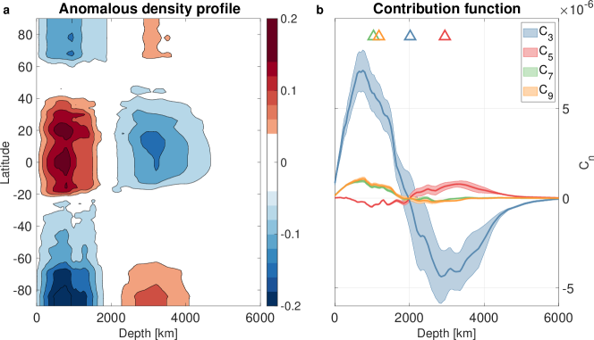
Figure 3: (a) The mean anomalous density profile of all possible decay options that fits the Juno four measured odd gravity harmonics; colors represent the anomalous density values $[{\rm kg\,~{}m^{-3}}]$. (b) Averaged contribution function (lines) $[{\rm m^{-1}}]$ for each of the odd gravity harmonics and their associated standard deviation (shading); triangles represent the depth of the mean anomaly. Both panels are for all the latitudes and for only the upper $\sim 6000$ km, below which the anomalous density is zero.

4 Sensitivity to the meridional profile of the zonal flows

Next, we relax the assumption, used in the previous section, that the meridional profile of Jupiter’s zonal flow remains constant at all depths. First, the zonal wind profile is measured by tracking cloud motion, which itself has some uncertainty (Tollefson et al.,, 2017). Second, and most importantly, the assumption that the cloud-level profile extends perfectly to depth along the direction of the spin axis requires the flow to be locally close-to-barotropic (in the upper few thousand kilometers), which is not necessarily the case. Although the flow cannot be completely barotropic if $Q_{s}\neq 1$ (Eq. 4), the horizontal density gradients required to balance the vertical changes associated with $Q_{s}$ may be small (Eq. 3). Any further deviation from close-to-barotropic flow must be supported by horizontal density (or temperature) gradients, which themselves must be maintained by some internal mechanism (Showman and Kaspi,, 2013). Internal convection models support the scenario that there may be internal shear over the upper few thousand kilometers, but the overall structure of the flow does not change much (Kaspi et al.,, 2009; Jones and Kuzanyan,, 2009). Any significant deviation from the zonal wind profile observed at the cloud level requires significant shear and, therefore, notable horizontal thermal gradients (thermal-wind balance). As this is an open question, for the purpose of this analysis, we examine several cases of zonal wind meridional profiles, under the assumption that the wind profile possibly varies close to the cloud level and then projects inward without further modifications. For the purpose of the gravity analysis, this means that the altered meridional profiles occupy enough mass to affect the gravity field, and the flow observed at the cloud level is limited to a shallow-enough layer so it does not affect the gravity field.

The simplest case is clearly to use the measured profile at Jupiter’s cloud level and allow its magnitude to decay with depth (section 3). A slightly less constraining option is to insert a perturbation into the measured profile, thereby keeping the general form and allowing a varying level of modifications to the cloud-level flow. The perturbed winds chosen here might represent the measured uncertainties in Jupiter’s cloud-level wind (Garcıa-Melendo and Sánchez-Lavega,, 2001; Tollefson et al.,, 2017). Finally, random meridional profiles of the zonal flow with a spectra generally similar to that of Jupiter are examined as well.

The modified zonal flow profile is chosen at the cloud level and projected inwards along the rotation axis ($u_{{\rm proj}}$, Eq. 4) with a range of vertical profiles, as described in section 3. The profiles are calculated by adding sinusoidal perturbations to the measured wind. The modified profiles have a standard deviation of $5\pm 0.5\,{\rm m~{}s^{-1}}$ (varies with latitude) relative to the cloud-level winds, well within the measurement error (Garcıa-Melendo and Sánchez-Lavega,, 2001; Tollefson et al.,, 2017). The perturbation is constructed as

$$\epsilon\left(\theta\right)={\sum}_{n=1}^{10}\left[a_{n}\sin\left(2n\theta\right)+b_{n}\cos\left(2n\theta\right)\right],$$ (8)

where $\epsilon$ is the perturbation and $a_{n}$ and $b_{n}$ are random numbers that are normally distributed around zero with a standard deviation of $2$ ${\rm m~{}s^{-1}}$. We first examine $1000$ modified profiles, each constructed by adding the perturbation to the measured wind (section 4.1). In addition, $1000$ random profiles are constructed purely from the $\epsilon$ function (Eq. 8), where $a_{n}$ and $b_{n}$ have a standard deviation of $30\,{\rm m~{}s^{-1}}$. These profiles represent internal winds that are completely unrelated to the observed cloud-level winds (section 4.2).

4.1 Perturbed cloud-level wind profiles

The perturbed wind profiles (Fig. 4a, colors) result in a substantially bigger solution envelope (Fig. 4b.1-4, gray) than the one from the measured zonal wind profile case, consistent with the fact that a wider range of wind profiles is allowed. Note that the overall shape has changed and that the flow can even vanish at $\sim 2500$ km. This might have an important implication, since the initial time-dependent magnetic field results from Juno imply that the wind at these depths are very weak (Duer et al.,, 2019; Moore et al.,, 2019). An important result is that even for the perturbed winds there are no solutions that fit at least three odd $J_{n}$ that vanish above $2000$ km. The depth sensitivity of each harmonic is less pronounced than for the measured wind case. This reflects the fact that Fig. 4 is a combination of all the possible solutions from $1000$ examined meridional structures. Overall, $J_{3}$ is still sensitive in the deeper regions (exemplified by the mean profile being weaker at depth, red line Fig. 4b.1), although $J_{7}$ and $J_{9}$ contribute at depth as well. $J_{5}$ turns out to be the most insignificant harmonic and $J_{9}$ does affect the depth range of $1500-2000$ km, unlike in the unperturbed wind case. The substantially larger range of solutions, however, does not manifest in more solutions relative to the examined cases. From $1000$ examined profiles individually tested with the decay sample population, only about $0.1\%$ fit the anomalous gravity field compared to about $1\%$ in the unperturbed case (Fig. 5, red and blue). This suggests that although perturbed cloud-level wind profiles are possible, it is statistically more likely that a profile that is similar to the projection of the observed cloud-level wind is indeed the profile in the deeper atmosphere of Jupiter.

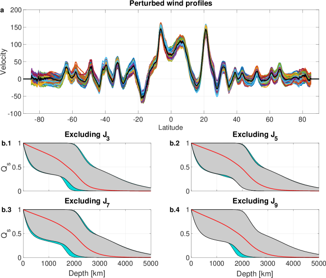
Figure 4: (a) 100 examples of the 1000 perturbed wind profiles (colors, [${\rm m~{}s^{-1}}$]) and Jupiter’s measured wind profile (black). (b.1-4) The odd gravity harmonics of the perturbed wind profiles depth sensitivity summary as in Fig. 2. Each profile is examined with the same set of decay options. The results shown here are for all meridional and vertical options combined.

4.2 The possibility of other zonal wind profiles

Next, we consider profiles that do not resemble Jupiter’s cloud-level winds (Fig. 6a). The resulting solution envelopes of the other zonal wind profiles are relatively similar to the previous case of perturbed winds (not shown). Only a very small subset of profiles ($13$ meridional profiles out of $1000$, about $1\%$) fit the four measured odd gravity harmonics (Fig. 6b.1). The possibility of fitting two or more odd harmonics is rare and exists in only $7\%$ or less of the zonal wind meridional profiles examined (Fig. 6b.2-3). $J_{3}$ is the harmonic that is pronounced in the majority of profiles (Fig. 6b.4). In $14\%$ of the examined random profiles, no odd harmonic is within the sensitivity range. In general, the measured harmonic’s alignment with the zonal flow structure does not appear to be coincidental. These findings are expected, considering that it is unlikely that an utterly different profile of zonal profiles arise below the cloud level of Jupiter.

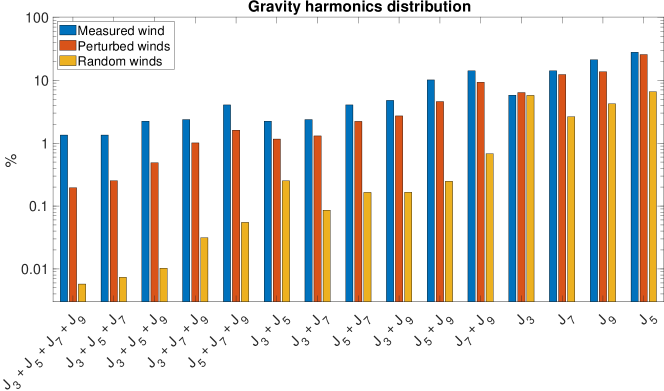
Figure 5: Summary of the solutions for the three presented cases of wind structures: Jupiter’s measured wind at the cloud level (blue), 1000 slightly modified meridional structures (red) and 1000 random meridional profiles with a similar general structure to Jupiter’s meridional profile (orange). The ordinate is a logarithmic scale of percentage relative to all the examined cases. The particular requirement of the solution to match the different odd gravity harmonics is presented by the abscissa.

The ability of the $1000$ examined random profiles, each with its sample of decay options, to fit all four odd gravity harmonics is considerably smaller than previous cases - only about $0.01\%$ (Fig. 5, orange). This indicates that fitting all four odd harmonics is difficult with random meridional profiles of zonal wind. A summary of the examined cases appears in Fig. 5. Note that the ordinate is a logarithmic scale and that $100\%$ stands for all the zonal profiles ($1000$ zonal wind profiles other than the measured cloud-level wind) and all decay options ($5\times 10^{5}$) for each case. We find that the envelope of possible solutions from Fig. 1 stands for $\sim 1\%$ of the tested vertical profiles for zonal flows. The fitting percentage decreases with increasing perturbations, and drops rapidly when switching to random profiles. This trend repeats for all variations of at least three odd harmonics. For all cases, the random winds show a significantly lower fitting percentage than the other cases. We further present the fitting percentage obtained following the exclusion of two and three harmonics. In summary, we find that other meridional profiles of the zonal wind are possible, but they are statistically unlikely. This result implies that the meridional profile of Jupiter’s zonal winds extends into the interior along the direction of the spin axis and weakens with depth, and is likely not significantly different from the cloud-level profile.

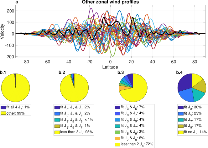
Figure 6: (a) 30 examples of the 1000 random zonal wind profiles examined (colors, [${\rm m~{}s^{-1}}$]) and Jupiter’s measured wind profile (black). (b.1-4) Summary of the random meridional profiles’ correspondence to the odd gravity harmonics. Only $\sim 1\%$ of the zonal profiles fit all four odd gravity harmonics (b.1), $5\%$ of the zonal profiles fit at least three odd gravity harmonics (b.2), $28\%$ of the zonal profiles fit at least two odd gravity harmonics (b.3) and $14\%$ do not fit any of the odd gravity harmonics (b.4). The full compatibility distribution is detailed in the figure.

5 Zonal wind profiles inspired by the MWR measurements

In addition to the gravity measurements, Juno’s six-channel microwave radiometer (MWR) measurements might also reveal information about the structure of the wind below the cloud level. These measurements are used to calculate the nadir brightness temperature ($T_{b}$), a profile determined by the opacity of the atmosphere, which in Jupiter is determined mostly by ammonia abundance (Li et al.,, 2017). The MWR measurements reveal considerable variation of $T_{b}$ with latitude and depth (Bolton et al.,, 2017) (Fig. 7a, black lines). These variations with depth and the potential relation between $T_{b}$ and the zonal jets (Ingersoll et al.,, 2017) suggest that Jupiter’s zonal jets might be depth-dependent, similarly to $T_{b}$, instead of simply projected inwards (as in sections 3 and 4).

One approach for describing the relation between the brightness temperature and the zonal jets is taking the brightness temperature as simply temperature. Then, the relation is described by the thermal wind balance, as discussed in section 2. This approach, however, results in equatorial wind that is greater by two orders of magnitude than the measured cloud-level wind, which is unrealistic (Bolton et al.,, 2017). Another approach is taking the brightness temperature as an indicator for ammonia concentration (Ingersoll et al.,, 2017) and examining the relation to the zonal jets. As an example, such a relation is expected in the meridional circulation (Ferrel cells), where the cell-associated vertical velocity redistribute the substance and is accompanied by zonal jets (Fletcher et al.,, 2020). Here, we take the latter approach, analyzing a range of depth-dependent meridional profiles, compatible with the brightness temperature variations with depth.

When examining the correlation between $T_{b}$ and the zonal jets, a different analysis should be taken at different latitudes, and perhaps at different depths. If the zonal jets are associated with multiple Ferrel cells in alternating directions associated with regions of momentum convergence (eastward jets) and divergence (westward jets), a correlation is expected between the zonal velocity and the ammonia concentration gradient. In such a scenario, the meridional cells advect the ammonia concentration, maximizing its gradient where the jet peaks (Fletcher et al.,, 2020). However, momentum fluxes converging at the equator would lead to a superrotating jet (Kaspi et al.,, 2009) and might also lead to a maximal ammonia concentration. Therefore, at the equator, the zonal velocity is associated with the concentration itself and not with its gradient. These simple considerations motivates us to examine the correlation both between $u$ and $\nabla T_{b}$ and between $u$ and $T_{b}$ (Table 1, columns 2 and 3). Note that, as in all our experiments, the zonal jets are projected inwards along the spin axis, as in section 3 (Fig. 7a, colors). It is evident that the correlation between $u$ and $T_{b}$ is weak at the cloud level (channel 6, $0.6$ bar), but become stronger with depth (maximum at channel 1, $240$ bar), while the correlation between $u$ and $\nabla T_{b}$ is strong at the cloud level, and weakens with depth (at channels 1-3, the correlation is weak). This alone might indicate two opposite meridional cells, one stacked on top of the other (Showman and de Pater,, 2005; Fletcher et al.,, 2020). At the cloud level, the correlation between $u$ and $\nabla T_{b}$ improves if we do not consider the equatorial region, which is consistent with the Ferrel cells hypothesis. Projecting the winds in the radial direction instead of along cylinders does not improve the correlation to neither $T_{b}$ or $\nabla T_{b}$ (Fig. 7b.1).

The dominant feature leading to the strong correlation between $u$ and $T_{b}$ at channel 1 is the equatorial anomaly, ascending at $\sim 15^{\circ}~{}\rm{S}$ and descending at $\sim 15^{\circ}~{}\rm{N}$ (Fig. 7b.1). While at the cloud level, both the zonal jets and $T_{b}$ reveal alternating patterns (Fig. 7b.6), the waviness of $T_{b}$ vanishes at deeper depths (Fig. 7b.1-2). Since $T_{b}$ is depth-dependent, getting smoother with depth from channel 6 (cloud level) to channel 1 ($\sim 300$ km depth), we examine zonal jets that are depth-dependent. Note that winds, projected along the spin axis, maintain their meridional profile with cylinders, and without further assumptions, are not depth-dependent. The modified (smoothed) wind at channel 1 is composed using a running average of $\Delta\theta$ degrees latitude, where $\Delta\theta=0,1,2,...,10^{\circ}$ ($0^{\circ}$ means that no running average is applied). The wind at channel 6 is the observed cloud-level profile; between channel 1 and channel 6, the wind strength is interpolated. Finally, the wind profile at the depth of $300$ km (channel 1) is projected inwards along the spin axis with a decay profile as in the previous sections without further assumptions. In addition to the projected winds with no depth-dependency ($\Delta\theta=0^{\circ}$, Fig. 7b, light blue), we examine the correlation between $u$ and $T_{b}$ for two cases of a depth-dependent zonal wind ($\Delta\theta=4^{\circ}$ and $\Delta\theta=8^{\circ}$, Fig. 7b, blue). Increasing the running average at depth improves the correlation at channels 1-3 (columns 3-5, Table 1), implying that the latitudinal variability of the jets might weaken beneath the cloud level.

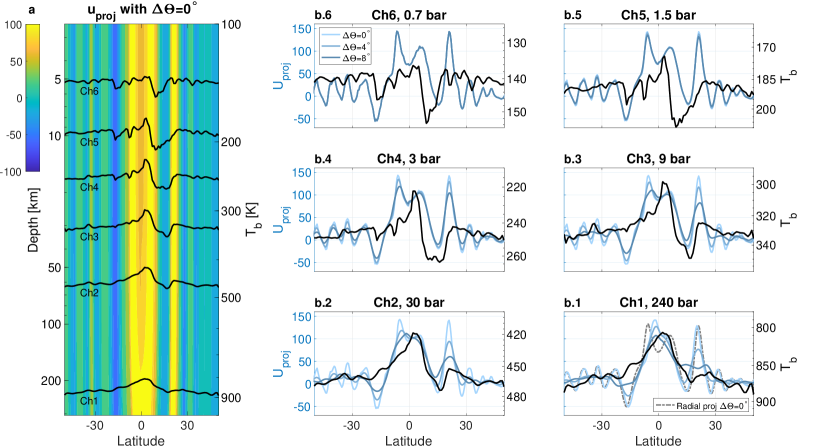
Figure 7: (a) Jupiter’s projected wind velocities (colors, [${\rm m~{}s^{-1}}$]) between latitudes $-50^{\circ}$ and $50^{\circ}$ in the upper $300$ km of Jupiter (left ordinate) combined with nadir brightness temperature lines from Juno’s PJ1 (black, right ordinate) in channels 1 to 6, associated with frequencies of $0.6$, $1.2$, $2.6$, $5.2$, $10$ and $22$ ${\rm GHz}$, respectively. (b.1-6) Jupiter’s projected wind velocities [${\rm m~{}s^{-1}}$] at channel 1 , $240$ bar (b.1), channel 2 , $30$ bar (b.2), channel 3, $9$ bar (b.3), channel 4, $3$ bar (b.4), channel 5, $1.5$ bar (b.5), and channel 6, $0.6$ bar (b.6) for a running average of $\Delta\theta=0^{\circ}$, $\Delta\theta=4^{\circ}$ and $\Delta\theta=8^{\circ}$ (darker blue with increasing $\Delta\theta$, left ordinate). Also shown is the brightness temperature [${}^{\circ}{\rm K}$] (black, right ordinate). The radial projection of the winds with no running average (dashed gray) is also presented in b.1.

Table 1: Correlation coefficients between $\nabla T_{b}$ and the wind velocity at each channel, for winds with no running average at depth ($\Delta\theta=0^{\circ}$), and correlation coefficients between $T_{b}$ and the wind velocity at the same depths with no running average ($\Delta\theta=0^{\circ}$), with running average of $4$ degrees ($\Delta\theta=4^{\circ}$), and with a running average of $8$ degrees ($\Delta\theta=8^{\circ}$). Note that for $u$ vs. $T_{b}$, the correlation increases with depth (or decreases with channel) and with running average.

	$u$ vs. $\nabla T_{b}$	$u$ vs. $T_{b}$
Channel	$\Delta\theta=0^{\circ}$	$\Delta\theta=0^{\circ}$	$\Delta\theta=4^{\circ}$	$\Delta\theta=8^{\circ}$
$1$	$0.05$	$0.64$	$0.76$	$0.86$
$2$	$0.02$	$0.74$	$0.80$	$0.84$
$3$	$0.01$	$0.63$	$0.65$	$0.68$
$4$	$0.15$	$0.41$	$0.41$	$0.42$
$5$	$0.24$	$0.13$	$0.13$	$0.13$
$6$	$0.42$	$0.10$	$0.10$	$0.10$

Next, we examine the ability of the depth-dependent zonal profiles to explain the measured odd gravity harmonics. We examine a range of case studies, from slightly to largely modified depth-dependent profiles, until no solutions are found (Fig. 8a). For slightly smoother profiles (small $\Delta\theta$), the ability to fit all four odd $J_{n}$ is similar to that without any smoothing ($\Delta\theta=0^{\circ}$) (Fig. 8a). Applying additional smoothing (increasing $\Delta\theta$) decreases the ability to fit the four odd $J_{n}$. Using more than a $10$-degree running average results in no solutions for the odd gravity harmonics. The three case studies ($\Delta\theta=0^{\circ}$, $\Delta\theta=4^{\circ}$ and $\Delta\theta=8^{\circ}$) show a consistent trend when excluding one of the odd harmonics, such that the ability to fit the gravity measurements is reduced when it comes to smoother deep profiles (Fig. 8b). This result is compatible with the previous case (section 4), indicating that deep wind that resembles the cloud-level wind can fit the gravity data, and changing the zonal wind structure considerably limits the ability to find a solution. The main conclusion of the analysis presented above is that wind profiles correlated with $T_{b}$ at depth ($\Delta\theta=4^{\circ}$) can adequately fit the gravity measurements.

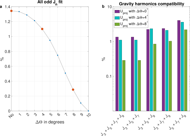
Figure 8: (a) The ability of the depth-dependent wind profiles to fit all four odd gravity harmonics (percentage of solutions) as a function of the smoothing factor in degrees (blue line). The three cases shown in Fig. 7b are denoted by red dots. (b) The gravity harmonics distribution for the red dots is compatible with the three case studies in Fig. 7b. The ordinate is a scale of percentage relative to the $5\times 10^{5}$ decay options examined.

6 Discussion and conclusions

The main challenge of interpreting the Juno gravity measurements is that the measurements provide only a handful of numbers (gravity harmonics), while the meridional and vertical profile of the interior flow have many degrees of freedom. Therefore, by-definition, the problem is ill-posed. Acknowledging this inherent issue, Kaspi et al., (2018) used four degrees of freedom for the vertical flow profile (matching the number of the four odd harmonics), and found the best optimized profile for this allowed range. They addressed the non-uniqueness by showing the statistical likelihood of wind profiles for the interior that are completely different than the cloud-level flow. Kong et al., (2018) highlighted the non-uniqueness issue by showing that two different flow profiles can still satisfy the gravity measurements. In this study, we take a more methodological approach and consider a wider range of solutions and analyze their statistical likelihood. The flow profiles we consider, both for the meridional and vertical profiles, are bound by physical considerations. We also address two main issues: First, all previous studies looked at all four odd gravity harmonics together, and found the flow profiles best matching all four. Here, we investigate how each one of them separately bounds the flow. Second, in an attempt to coincide the gravity and microwave data, we explore whether deep profiles that are smoother than those of the cloud-level, as possibility indicated by the Juno microwave measurements, can be consistent with the gravity measurements.

By assuming that the cloud-level wind profile is projected inwards parallel to the spin axis, with some decay profile, we identify the envelope of possible solutions (Fig. 1). We then relax the dependence on each of the odd gravity harmonics separately and analyze their individual contribution to the vertical profile of the zonal wind (Fig. 2). We find that $J_{3}$, the lowest order odd harmonic that represents the dynamics of Jupiter, is sensitive at depths where the conductivity rises (beyond $\sim 3000$ km), and the magnetic field might be interacting with the flow, resulting in the Lorentz force playing a key role in the dynamics. $J_{5}$ appears to be the most sensitive harmonic, giving a robust constraint on the vertical profile of the zonal flow alone (Fig. 2b). Interestingly, $J_{9}$ does not give any new constraint on the flow if the other three harmonics are within the sensitivity range (Fig. 2d). A possible explanation for the unique nature of $J_{5}$ comes from exploring the contribution function, which revealed that $J_{5}$ is most sensitive in the deeper regions, below $2000$ km (Fig. 3).

The modified zonal flow analysis revealed a substantially bigger possible solution envelope than that obtained by extending the cloud-level wind (Fig. 4). This implies that the zonal wind’s structure may influence the depth sensitivity of each harmonic. Even for the perturbed winds, the flow cannot vanish at depths shallower than $2000$ km. The case with random winds implies that, with high probability, the wind cannot alter completely below the cloud level. Fitting the four odd gravity harmonics (or three if we ignore $J_{9}$) requires either similar winds to the measured ones at the cloud level, that would penetrate a few thousand kilometers into the planet, or a very specific and statistically unlikely combination of a meridional and a decay profiles (Fig. 5, 6). Finally, the gravity harmonics induced by the slightly modified depth-dependent meridional profiles, which have a better correlation with the MWR measurements at depth (Fig. 7, Table 1), are still within Juno’s gravity measurements’ uncertainty, indicating that Jupiter’s ammonia abundance could indeed reflect the profile of the zonal jet at 300 km (Fig. 8).

Acknowledgments:

We thank Cheng Li for providing the MWR data. This research has been supported by the Israeli Space Agency and the Helen Kimmel Center for Planetary Science at the Weizmann Institute of Science. The Juno gravity measurements and MWR measurements are publicly available, see https://pds-atmospheres.nmsu.edu/data_and_services/atmospheres_data/JUNO/juno.html. Additional data can be found here https://doi.org/10.5281/zenodo.3859828.

References

- Fletcher et al., (2020) Fletcher, L. N. and Kaspi, Y. and Guillot, T. and Showman, A. P. How well do we understand the belt/zone circulation of Giant Planet atmospheres?. (2020). Space Sci. Rev., 216:1–33.
- Showman and de Pater, (2005) Showman, A. P. and de Pater, I. (2005). Dynamical implications of Jupiter’s tropospheric ammonia abundance. Icarus, 174:192–204.
- Kaspi et al., (2017) Kaspi, Y and Galanti, E. and Showman, A. P. and Stevenson, D. J. and Guillot, T. and Iess, L. and Bolton. S. J. (2020). Comparison of the deep atmospheric dynamics of Jupiter and Saturn in light of the Juno and Cassini gravity measurements. Space Sci. Rev.. In press.
- Bolton et al., (2017) Bolton, S. J., Adriani, A., Adumitroaie, V., Allison, M., Anderson, J., Atreya, S., Bloxham, J., Brown, S., Connerney, J. E. P., DeJong, E., Folkner, W., Gautier, D., Grassi, D., Gulkis, S., Guillot, T., Hansen, C., Hubbard, W. B., Iess, L., Ingersoll, A., Janssen, M., Jorgensen, J., Kaspi, Y., Levin, S. M., Li, C., Lunine, J., Miguel, Y., Mura, A., Orton, G., Owen, T., Ravine, M., Smith, E., Steffes, P., Stone, E., Stevenson, D., Thorne, R., Waite, J., Durante, D., Ebert, R. W., Greathouse, T. K., Hue, V., Parisi, M., Szalay, J. R., and Wilson, R. (2017). Jupiter’s interior and deep atmosphere: The initial pole-to-pole passes with the Juno spacecraft. Science, 356:821–825.
- Busse, (1976) Busse, F. H. (1976). A simple model of convection in the Jovian atmosphere. Icarus, 29:255–260.
- Cao and Stevenson, (2017) Cao, H. and Stevenson, D. J. (2017). Zonal flow magnetic field interaction in the semi-conducting region of giant planets. Icarus, 296:59–72.
- Duer et al., (2019) Duer, K., Galanti, E., and Kaspi, Y. (2019). Analysis of Jupiter’s deep jets combining Juno gravity and time-varying magnetic field measurements. Astrophys. J. Let., 879(2):L22.
- French et al., (2012) French, M., Becker, A., Lorenzen, W., Nettelmann, N., Bethkenhagen, M., Wicht, J., and Redmer, R. (2012). Ab initio simulations for material properties along the Jupiter adiabat. Astrophys. J. Sup., 202:5.
- (9) Galanti, E., Cao, H., and Kaspi, Y. (2017a). Constraining Jupiter’s internal flows using Juno magnetic and gravity measurements. Geophys. Res. Lett., 44:8173–8181.
- (10) Galanti, E., Kaspi, Y., and Tziperman, E. (2017b). A full, self-consistent, treatment of thermal wind balance on fluid planets. J. Comp. Phys., 810:175–195.
- Garcıa-Melendo and Sánchez-Lavega, (2001) Garcıa-Melendo, E. and Sánchez-Lavega, A. (2001). A study of the stability of jovian zonal winds from HST images: 1995–2000. Icarus, 152(2):316–330.
- Gastine et al., (2014) Gastine, T., Wicht, J., Duarte, L. D. V., Heimpel, M., and Becker, A. (2014). Explaining Jupiter’s magnetic field and equatorial jet dynamics. Geophys. Res. Lett., 41:5410–5419.
- Guillot and Gautier, (2007) Guillot, T. and Gautier, D. (2007). Treatise of Geophysics: 10. Planets and Moons, chapter Giant planets, pages 439–464. Elsevier.
- Guillot et al., (2018) Guillot, T., Miguel, Y., Militzer, B., Hubbard, W. B., Kaspi, Y., Galanti, E., Cao, H., Helled, R., Wahl, S. M., Iess, L., Folkner, W. M., Stevenson, D. J., Lunine, J. I., Reese, D. R., Biekman, A., Parisi, M., Durante, D., Connerney, J. E. P., Levin, S. M., and Bolton, S. J. (2018). A suppression of differential rotation in Jupiter’s deep interior. Nature, 555:227–230.
- Helled et al., (2010) Helled, R., Anderson, J. D., Podolak, M., and Schubert, G. (2010). Interior models of Uranus and Neptune. Astrophys. J., 726(1):15.
- Hubbard, (1984) Hubbard, W. B. (1984). Planetary Interiors. pp. 343. New York, Van Nostrand Reinhold Co.
- Hubbard, (1999) Hubbard, W. B. (1999). Note: Gravitational signature of Jupiter’s deep zonal flows. Icarus, 137:357–359.
- Hubbard, (2012) Hubbard, W. B. (2012). High-precision Maclaurin-based models of rotating liquid planets. Astrophys. J. Let., 756:L15.
- Hubbard et al., (1975) Hubbard, W. B., Slattery, W. L., and Devito, C. L. (1975). High zonal harmonics of rapidly rotating planets. Astrophys. J., 199:504–516.
- Hubbard et al., (1974) Hubbard, W. B., Trubitsyn, V. P., and Zharkov, V. N. (1974). Significance of gravitational moments for interior structure of Jupiter and Saturn. Icarus, 21(2):147–151.
- Iess et al., (2018) Iess, L., Folkner, W. M., Durante, D., Parisi, M., Kaspi, Y., Galanti, E., Guillot, T., Hubbard, W. B., Stevenson, D. J., Anderson, J. D., Buccino, D. R., Casajus, L. G., Milani, A., Park, R., Racioppa, P., Serra, D., Tortora, P., Zannoni, M., Cao, H., Helled, R., Lunine, J. I., Miguel, Y., Militzer, B., Wahl, S., Connerney, J. E. P., Levin, S. M., and Bolton, S. J. (2018). Measurement of Jupiter’s asymmetric gravity field. Nature, 555(7695):220–222.
- Ingersoll et al., (2017) Ingersoll, A. P., Adumitroaie, V., Allison, M. D., Atreya, S., Bellotti, A. A., Bolton, S. J., Brown, S. T., Gulkis, S., Janssen, M. A., Levin, S. M., Cheng, L., Liming, L., Lunine, J. I., Orton, G. S., Oyafuso, F. A., and Steffes, P. G. (2017). Implications of the ammonia distribution on Jupiter from 1 to 100 bars as measured by the Juno microwave radiometer. Geophys. Res. Lett., 44(15):7676–7685.
- Jones and Kuzanyan, (2009) Jones, C. A. and Kuzanyan, K. M. (2009). Compressible convection in the deep atmospheres of giant planets. Icarus, 204:227–238.
- Kaspi, (2013) Kaspi, Y. (2013). Inferring the depth of the zonal jets on Jupiter and Saturn from odd gravity harmonics. Geophys. Res. Lett., 40:676–680.
- Kaspi et al., (2016) Kaspi, Y., Davighi, J. E., Galanti, E., and Hubbard, W. B. (2016). The gravitational signature of internal flows in giant planets: comparing the thermal wind approach with barotropic potential-surface methods. Icarus, 276:170–181.
- Kaspi et al., (2009) Kaspi, Y., Flierl, G. R., and Showman, A. P. (2009). The deep wind structure of the giant planets: Results from an anelastic general circulation model. Icarus, 202:525–542.
- Kaspi et al., (2018) Kaspi, Y., Galanti, E., Hubbard, W. B., Stevenson, D. J., Bolton, S. J., Iess, L., Guillot, T., Bloxham, J., Connerney, J. E. P., Cao, H., Durante, D., Folkner, W. M., Helled, R., Ingersoll, A. P., Levin, S. M., Lunine, J. I., Miguel, Y., Militzer, B., Parisi, M., and Wahl, S. M. (2018). Jupiter’s atmospheric jet-streams extend thousands of kilometers deep. Nature, 555:223–226.
- Kaspi et al., (2010) Kaspi, Y., Hubbard, W. B., Showman, A. P., and Flierl, G. R. (2010). Gravitational signature of Jupiter’s internal dynamics. Geophys. Res. Lett., 37:L01204.
- Kong et al., (2018) Kong, D., Zhang, K., Schubert, G., and Anderson, J. D. (2018). Origin of Jupiter’s cloud-level zonal winds remains a puzzle even after Juno. Proc. Natl. Acad. Sci. U.S.A., 115(34):8499–8504.
- Li et al., (2017) Li, C., Ingersoll, A., Janssen, M., Levin, S., Bolton, S., Adumitroaie, V., Allison, M., Arballo, J., Bellotti, A., Brown, S., Ewald, S., Jewell, L., Misra, S., Orton, G., Oyafuso, F., Steffes, P., and Williamson, R. (2017). The distribution of ammonia on Jupiter from a preliminary inversion of Juno microwave radiometer data. Geophys. Res. Lett., 44(11):5317–5325.
- Liu et al., (2008) Liu, J., Goldreich, P. M., and Stevenson, D. J. (2008). Constraints on deep-seated zonal winds inside Jupiter and Saturn. Icarus, 196:653–664.
- Moore et al., (2019) Moore, K. M., Cao, H., Bloxham, J., Stevenson, D. J., Connerney, J. E., and Bolton, S. J. (2019). Time-variation of Jupiter’s internal magnetic field consistent with zonal wind advection. Nature Astronomy, page 1.
- Nellis et al., (1992) Nellis, W. J., Mitchell, A. C., McCandless, P. C., Erskine, D. J., and Weir, S. T. (1992). Electronic energy gap of molecular hydrogen from electrical conductivity measurements at high shock pressures. Phys. Rev. Let., 68(19):2937.
- Nellis et al., (1996) Nellis, W. J., Weir, S. T., and Mitchell, A. C. (1996). Metallization and electrical conductivity of hydrogen in Jupiter. Science, 273(5277):936–938.
- Nettelmann et al., (2013) Nettelmann, N., Helled, R., Fortney, J. J., and Redmer, R. (2013). New indication for a dichotomy in the interior structure of Uranus and Neptune from the application of modified shape and rotation data. Planatary and Space Science.
- Nettelmann et al., (2013) Nettelmann, N., Püstow, R., and Redmer, R. (2013). Saturn layered structure and homogeneous evolution models with different eoss. Icarus, 225(1):548–557.
- Pedlosky, (1987) Pedlosky, J. (1987). Geophysical Fluid Dynamics. pp. 710. Springer-Verlag.
- Salyk et al., (2006) Salyk, C., Ingersoll, A. P., Lorre, J., Vasavada, A., and Del Genio, A. D. (2006). Interaction between eddies and mean flow in Jupiter’s atmosphere: Analysis of Cassini imaging data. Icarus, 185:430–442.
- Showman and Kaspi, (2013) Showman, A. P. and Kaspi, Y. (2013). Atmospheric dynamics of brown dwarfs and directly imaged giant planets. Astrophys. J., 776:85–103.
- Tollefson et al., (2017) Tollefson, J., Wong, M. H., de Pater, I., Simon, A. A., Orton, G. S., Rogers, J. H., Atreya, S. K., C., R. G., Januszewski, W., Morales-Juberías, R., and S., M. P. (2017). Changes in Jupiter’s zonal wind profile preceding and during the Juno mission. Icarus, 296:163–178.
- Weir et al., (1996) Weir, S. T., Mitchell, A. C., and Nellis, W. J. (1996). Metallization of fluid molecular hydrogen at 140 GPa (1.4 mbar). Phys. Rev. Let., 76:1860–1863.
- (42) Wicht, J., Gastine, T., and Duarte, L. D. (2019a). Dynamo action in the steeply decaying conductivity region of Jupiter-like dynamo models. J. Geophys. Res. (Planets), 124(3):837–863.
- (43) Wicht, J., Gastine, T., Duarte, L. D., and Dietrich, W. (2019b). Dynamo action of the zonal winds in Jupiter. Astron. and Astrophys., 629:A125.