Average nonlinear dynamics of particles in gravitational pulses: effective Hamiltonian, secular acceleration, and gravitational susceptibility

Abstract

Particles interacting with a prescribed quasimonochromatic gravitational wave (GW) exhibit secular (average) nonlinear dynamics that can be described by Hamilton’s equations. We derive the Hamiltonian of this “ponderomotive” dynamics to the second order in the GW amplitude for a general background metric. For the special case of vacuum GWs, we show that our Hamiltonian is equivalent to that of a free particle in an effective metric, which we calculate explicitly. We also show that already a linear plane GW pulse displaces a particle from its unperturbed trajectory by a finite distance that is independent of the GW phase and proportional to the integral of the pulse intensity. We calculate the particle displacement analytically and show that our result is in agreement with numerical simulations. We also show how the Hamiltonian of the nonlinear averaged dynamics naturally leads to the concept of the linear gravitational susceptibility of a particle gas with an arbitrary phase-space distribution. We calculate this susceptibility explicitly to apply it, in a follow-up paper, toward studying self-consistent GWs in inhomogeneous media within the geometrical-optics approximation.

I Introduction

Recent detection of gravitational waves (GWs) ref:abbott16a ; ref:abbott16b ; ref:abbott17a ; ref:abbott17b ; ref:abbott17c ; ref:abbott17d ; ref:abbott19 ; ref:abbott20a ; tex:abbott20b is strengthening the interest of the physics community in GW–matter interactions. Linear effects of GWs have long been studied in literature ref:zeldovich74 ; ref:braginskii85 ; ref:braginsky87 , particularly in the context of GW dispersion in gases and plasmas ref:chesters73 ; ref:asseo76 ; ref:macedo83 ; ref:servin01 ; ref:moortgat03 ; ref:forsberg10a ; ref:barta18 . Some authors have also explored the associated nonlinear phenomena, such as nonlinear memory effects ref:blanchet92 ; ref:christodoulou91 ; ref:thorne92 ; ref:wiseman91 ; ref:zhang18 ; ref:zhang17 ; ref:flanagan19 , the contribution of the GW tail from backscattering off the background curvature ref:blanchet92 ; ref:wiseman93 , and certain GW–plasma interactions ref:ignatev97 ; ref:brodin99 ; ref:brodin00 ; ref:brodin00b ; ref:papadopolous01 ; ref:brodin01 ; ref:balakin03c ; ref:servin03a ; ref:kallberg04 ; ref:vlahos04 ; ref:brodin05 ; ref:duez05a ; ref:isliker06 ; ref:forsberg06 ; ref:farris08 ; ref:forsberg08 ; ref:brodin10b . However, there remains another fundamental nonlinear effect, the “ponderomotive” effect, that is well-known for electromagnetic interactions ref:gaponov58 ; ref:motz67 ; ref:cary81 ; my:mneg ; my:qdirpond but has not yet received due attention in GW research. Like the aforementioned memory effects that have been known, the ponderomotive effect is hereditary, i.e., depends on the whole GW-intensity profile. But unlike the known memory effects, the ponderomotive effect is determined by the particle-motion equations (not the Einstein equations), so it can be produced even by linear GWs propagating in flat background spacetime.

The essence of the ponderomotive effect by GWs is as follows. Since the particle motion equations in a given metric are nonlinear, a prescribed GW generally induces not just quiver but also secular (average) nonlinear dynamics, regardless of whether the wave itself is linear or not. This nonlinear dynamics of particles is generally too complicated to study analytically; but it can be made tractable for quasimonochromatic GWs. In this case, the particle average motion can be described by relatively simple Hamilton’s equations, with a Hamiltonian that depends on the GW envelope and not on the GW phase. To the lowest order, the GW contribution to this Hamiltonian is of the second order in the wave amplitude. The resulting perturbations to the particle trajectories can be significant near sources of gravitational radiation, where the metric oscillations are substantial. These perturbations can also be important when particles are exposed to GWs long enough, since the ponderomotive effect is phase-independent and cumulative (see below). Furthermore, the ponderomotive effect is inherently related to the linear susceptibility of matter with respect to GWs. The corresponding statement for electromagnetic interactions is known as the $K$-$\chi$ theorem in plasma theory ref:cary77 ; ref:kaufman87 and has also been extended to more general Hamiltonian systems ref:kentwell87b ; my:kchi ; my:lens ; my:qponder . Hence, calculating the ponderomotive effect readily yields not just nonlinear forces on particles (which may or may not be significant in practice) but also linear dispersive properties of GWs in gases and plasmas. In this sense, the ponderomotive effect matters even in linear theory.

Here, we calculate the ponderomotive effect by weak GWs on neutral particles in the general case, i.e., when the GW envelope, wavevector, polarization, and background metric are arbitrary smooth functions of spacetime coordinates. Such general calculations are not easy to do by directly averaging the particle-motion equations, so we invoke variational methods that were recently developed within plasma theory for electromagnetic interactions my:itervar ; my:bgk ; my:acti ; my:sharm . We derive the Hamiltonian of the particle ponderomotive dynamics to the second order in the GW amplitude. For the special case of vacuum GWs, we show that our Hamiltonian is equivalent to that of a free particle in an effective metric, which we calculate explicitly. We also show that already a linear plane GW pulse displaces a particle from its unperturbed trajectory by a finite distance that is independent of the GW phase and proportional to the integral of the pulse intensity. In this sense, the ponderomotive effect is cumulative. We calculate the particle displacement analytically and show that our result is in agreement with numerical simulations. We also show how our general Hamiltonian yields the linear gravitational susceptibility of a particle gas with an arbitrary phase-space distribution. We calculate this susceptibility explicitly to apply it, in a follow-up paper, toward studying self-consistent GWs in inhomogeneous media within the geometrical-optics approximation.

Our paper is organized as follows. In Sec. II, we discuss the well-known equations of the particle motion in a prescribed metric, which we use later on. In Sec. III, we introduce the so-called oscillation-center formalism, which we build upon, by analogy with how this is done for electromagnetic interactions in plasma theory. In Sec. IV, we calculate the ponderomotive Hamiltonian and the ensuing equations of the average motion of a point particle. In Sec. V, we present an alternative derivation of the same ponderomotive Hamiltonian by treating particles as semiclassical quantum waves. We also apply these results to derive the gravitational susceptibility of a neutral gas. In Sec. VI, we discuss the particle motion in a linear vacuum GW pulse as an example, and we derive the total displacement of a particle under the influence of such a pulse. In Sec. VII, we present test-particle simulations, which show good agreement with our analytic theory. In Sec. VIII, we summarize our main results. Supplementary calculations are given in appendices. In particular, Appendix A details the derivation of a general theorem used in Sec. V.2, and Appendix B provides the derivation of an alternative form of the gravitational susceptibility introduced in Sec. V.5.

II Particle motion equations

II.1 Basic equations

Let us start with reviewing the known equations of the particle motion in a prescribed spacetime metric $g_{\alpha\beta}(x)$. We assume units such that the speed of light equals one ($c=1$), and the metric signature is assumed to be $(-+++)$. Then, the action $S$ of a particle traveling between two fixed spacetime locations $x_{1,2}\doteq x(\tau_{1,2})$ is given by

$$S=-m\int_{\tau_{1}}^{\tau_{2}}\sqrt{-g_{\alpha\beta}u^{\alpha}u^{\beta}}\,\mathrm{d}\tau.$$ (1)

Here, the symbol $\doteq$ denotes definitions, $m$ is the particle mass, $u^{\alpha}\doteq\mathrm{d}x^{\alpha}/\mathrm{d}\tau$ is the particle four-velocity, $u_{\alpha}\doteq g_{\alpha\beta}u^{\beta}$, and the proper time $\tau$ is defined such that

$$u_{\alpha}u^{\alpha}=-1.$$ (2)

Equation (2) serves as a constraint on the variational principle that governs the particle motion. Deriving the motion equations rigorously for a constrained action can be a subtle issue. However, we can sidestep this issue by rewriting Eq. (1) as an unconstrained action of the form

$$S=-m\int_{\tau_{1}}^{\tau_{2}}\,\mathrm{d}\tau,$$ (3)

with $\mathrm{d}\tau=\sqrt{-g_{\alpha\beta}\mathrm{d}x^{\alpha}\mathrm{d}x^{\beta}}$. Since this $S$ is not quite of the usual form $\int\mathscr{L}(x,\mathrm{d}x/\mathrm{d}\sigma)\,\mathrm{d}\sigma$, the resulting motion equations are not quite the standard Euler–Lagrange equations either. However, these equations still can be derived straightforwardly. Below, we describe two known approaches to this problem in detail, because we will need to refer to details of these approaches in later sections.

II.2 Covariant equations of motion

One way to derive the particle-motion equations from Eq. (3) is to proceed as follows book:landau2 . Consider a variation $x^{\mu}\to x^{\mu}+\delta x^{\mu}$ such that

$$\delta x^{\mu}(\tau_{1})=\delta x^{\mu}(\tau_{2})=0.$$ (4)

Then the variation of $S$ given by Eq. (3) can be written as

$$\delta S =-m\int_{\tau_{1}}^{\tau_{2}}\delta\,\mathrm{d}\tau$$

$$=m\int_{\tau_{1}}^{\tau_{2}}\frac{1}{2\mathrm{d}\tau}\,\delta\left(g_{\alpha\beta}\,\mathrm{d}x^{\alpha}\,\mathrm{d}x^{\beta}\right)$$

$$=m\int_{\tau_{1}}^{\tau_{2}}\frac{1}{2\mathrm{d}\tau}\left(\frac{\partial g_{\alpha\beta}}{\partial x^{\mu}}\,\delta x^{\mu}\,\mathrm{d}x^{\alpha}\,\mathrm{d}x^{\beta}+2g_{\alpha\beta}\,\mathrm{d}x^{\alpha}\,\mathrm{d}\delta x^{\beta}\right)$$

$$=m\int_{\tau_{1}}^{\tau_{2}}\left(\frac{1}{2}\frac{\partial g_{\alpha\beta}}{\partial x^{\mu}}\,u^{\alpha}u^{\beta}-\frac{\mathrm{d}u_{\mu}}{\mathrm{d}\tau}\right)\delta x^{\mu}\,\mathrm{d}\tau.$$ (5)

[Here, we have used symmetry of $g_{\alpha\beta}$; we have also integrated by parts to obtain the last equality and used Eq. (4) to eliminate the boundary term.] Then, the requirement that $\delta S=0$ for all $\delta x^{\mu}$ leads to the “geodesic equation”:

$$\frac{\mathrm{d}u_{\mu}}{\mathrm{d}\tau}=\frac{1}{2}\frac{\partial g_{\alpha\beta}}{\partial x^{\mu}}\,u^{\alpha}u^{\beta}.$$ (6)

Equations (6) can be viewed as the Euler–Lagrange equations corresponding to the Lagrangian

$$L(x,u)=\frac{m}{2}\,[g_{\alpha\beta}(x)u^{\alpha}u^{\beta}-1].$$ (7)

The second term is constant and could be omitted, but we have introduced it to keep $L=-m$ on solutions [due to Eq. (2); this is consistent with Eq. (3)] and to emphasize parallels with the calculations in the later sections. Let us also introduce the corresponding canonical momentum

$$p_{\alpha}\doteq\frac{\partial L}{\partial u^{\alpha}}=mu_{\alpha}$$ (8)

and the Hamiltonian $H\doteq p_{\alpha}u^{\alpha}-L$, or

$$H(x,p)=\frac{1}{2m}\,[g^{\alpha\beta}(x)p_{\alpha}p_{\beta}+m^{2}],$$ (9)

where $g^{\alpha\beta}$ is the inverse of the metric, $g^{\alpha\mu}g_{\mu\beta}=\delta^{\alpha}_{\beta}$. (In later sections, we show how this Hamiltonian emerges more naturally from first principles.) The corresponding Hamilton’s equations, equivalent to Eq. (6), are

$$\frac{\mathrm{d}x^{\alpha}}{\mathrm{d}\tau}=\frac{\partial H}{\partial p_{\alpha}},\quad\frac{\mathrm{d}p_{\alpha}}{\mathrm{d}\tau}=-\frac{\partial H}{\partial x^{\alpha}},$$ (10)

or explicitly,

$$\frac{\mathrm{d}x^{\alpha}}{\mathrm{d}\tau}=\frac{g^{\alpha\beta}p_{\beta}}{m},\quad\frac{\mathrm{d}p_{\alpha}}{\mathrm{d}\tau}=-\frac{1}{2m}\frac{\partial g^{\mu\nu}}{\partial x^{\alpha}}\,p_{\mu}p_{\nu}.$$ (11)

II.3 Non-covariant equations of motion

Another way to avoid dealing with the constraint (2) is to give up covariance of the motion equations and consider only the spatial dynamics instead ref:cognola86 ; foot:pmotion . Let us use Eq. (2) to express $u^{0}$ as a function of $t\doteq x^{0}$, $x^{a}$, and

$$v^{a}\doteq\frac{\mathrm{d}x^{a}}{\mathrm{d}t}=\frac{u^{a}}{u^{0}}.$$ (12)

Specifically, $u^{0}=\mathsf{u}^{0}(t,{\boldsymbol{\rm x}},{\boldsymbol{\rm v}})$, where

$$(\mathsf{u}^{0})^{-1}=\sqrt{-g_{ab}v^{a}v^{b}-2g_{0b}v^{b}-g_{00}}.$$ (13)

(Roman indices span from 1 to 3, unlike Greek indices, which span from 0 to 3. We also use bold font to denote three-dimensional spatial variables in the index-free form.) From Eq. (11), one has $\mathrm{d}t/\mathrm{d}\tau=u^{0}$, so $S$ can be written as a functional of only the spatial variables, $S=\int L_{t}\,\mathrm{d}t$, where $L_{t}=-m/\mathsf{u}^{0}$. In this representation, the action is unconstrained, so the motion equations are the usual Euler–Lagrange equations,

$$\frac{\mathrm{d}}{\mathrm{d}t}\left(\frac{\partial L_{t}}{\partial v^{a}}\right)=\frac{\partial L_{t}}{\partial x^{a}}.$$ (14)

Let us also introduce the corresponding Hamiltonian formulation. The canonical momenta are defined as $p_{a}=\smash{\partial L_{t}/\partial v^{a}}$, so $p_{a}=m\smash{\mathsf{u}^{0}}(g_{a0}+\smash{g_{ab}v^{b}})$, or equivalently,

$$p_{a}=m\left(g_{a0}\,\frac{\mathrm{d}x^{0}}{\mathrm{d}\tau}+g_{ab}\,\frac{\mathrm{d}x^{b}}{\mathrm{d}\tau}\right)=mg_{a\mu}u^{\mu},$$ (15)

where we used $\mathsf{u}^{0}=\mathrm{d}t/\mathrm{d}\tau$. Therefore, these momenta are the same as the corresponding spatial components of the four-vector canonical momenta (8). Let us also consider $p^{0}=mu^{0}$ and $p_{0}=mg_{0\mu}u^{\mu}$ as functions of $(t,{\boldsymbol{\rm x}},{\boldsymbol{\rm p}})$ and denote them as $\mathsf{p}^{0}(t,{\boldsymbol{\rm x}},{\boldsymbol{\rm p}})$ and $\mathsf{p}_{0}(t,{\boldsymbol{\rm x}},{\boldsymbol{\rm p}})$ respectively,

$$\mathsf{p}^{0}=m\mathsf{u}^{0},\quad\mathsf{p}_{0}=m\mathsf{u}_{0},$$ (16)

where the latter satisfies

$$H(t,{\boldsymbol{\rm x}},\mathsf{p}_{0}(t,{\boldsymbol{\rm x}},{\boldsymbol{\rm p}}),{\boldsymbol{\rm p}})=0.$$ (17)

Using Eq. (2), we can find the explicit expressions for $\mathsf{p}^{0}(t,{\boldsymbol{\rm x}},{\boldsymbol{\rm p}})$ and $\mathsf{p}_{0}(t,{\boldsymbol{\rm x}},{\boldsymbol{\rm p}})$. In order to proceed, consider

$$\sigma^{ab}\doteq g^{ab}-g^{a0}g^{b0}/g^{00}.$$ (18)

Then, one can show that foot:pmotion

$$\mathsf{p}^{0}(t,{\boldsymbol{\rm x}},{\boldsymbol{\rm p}})=m\gamma\sqrt{-g^{00}},$$ (19)

$$\mathsf{p}_{0}(t,{\boldsymbol{\rm x}},{\boldsymbol{\rm p}})=-\frac{m\gamma}{\sqrt{-g^{00}}}-\frac{g^{0a}}{g^{00}}\,p_{a},$$ (20)

where $\gamma\doteq\sqrt{1+\sigma^{ab}p_{a}p_{b}/m^{2}}$. One can further find the Hamiltonian of the spatial motion $H_{t}\doteq p_{a}v^{a}-L_{t}$ to be

$$H_{t}(t,{\boldsymbol{\rm x}},{\boldsymbol{\rm p}})=-\mathsf{p}_{0}(t,{\boldsymbol{\rm x}},{\boldsymbol{\rm p}}).$$ (21)

The corresponding Hamilton’s equations are

$$\frac{\mathrm{d}x^{a}}{\mathrm{d}t}=\frac{\partial H_{t}}{\partial p_{a}},\quad\frac{\mathrm{d}p_{a}}{\mathrm{d}t}=-\frac{\partial H_{t}}{\partial x^{a}}.$$ (22)

As can be checked, these equations are in agreement with the covariant Hamilton’s equations (11).

III Particles in an oscillating metric: basic concepts

III.1 Metric model

Let us suppose a metric in the form

$$g_{\alpha\beta}=\bar{g}_{\alpha\beta}+h_{\alpha\beta}.$$ (23)

Here, $\bar{g}_{\alpha\beta}=\bar{g}_{\alpha\beta}(\epsilon x)$ is a slow function of the spacetime coordinates $x$ and $h_{\alpha\beta}$ is a quasimonochromatic perturbation, i.e., can be expressed as $h_{\alpha\beta}=h_{\alpha\beta}[\epsilon x,\theta(x)]$, where $\epsilon$ is a small parameter and the dependence on the scalar “phase” $\theta$ is $2\pi$-periodic. We also assume

$$h_{\alpha\beta}\ll 1,\quad\langle h_{\alpha\beta}\rangle_{\theta}=0,$$ (24)

where $\langle\ldots\rangle_{\theta}$ denotes average over $\theta$. Then, $\bar{g}_{\alpha\beta}$ can be understood as the $\theta$-average part of the total metric,

$$\bar{g}_{\alpha\beta}=\langle g_{\alpha\beta}\rangle_{\theta}.$$ (25)

We shall attribute such metric perturbation as a GW. Note that

$$k_{\alpha}\doteq\partial_{\alpha}\theta=\nabla_{\alpha}\theta$$ (26)

can be interpreted as the local wavevector and $\epsilon$ can be interpreted as the geometrical-optics (GO) parameter, which is roughly

$$\epsilon\sim\lambda/\ell\ll 1.$$ (27)

Here, $\lambda$ is the characteristic wavelength (in spacetime) and $\ell\sim[\min\{\partial\bar{g}(\epsilon x),\partial h(\epsilon x,\theta),\partial\lambda(\epsilon x)\}]^{-1}$ is the characteristic inhomogeneity scale (in spacetime) of the background metric, GW envelope, and GW wavelength.

Note that the GW is not assumed linear. The quasiperiodic functions $\smash{h_{\alpha\beta}}$ may contain multiple harmonics, and any secular nonlinearity can be absorbed in the background metric $\smash{\bar{g}_{\alpha\beta}}$. Hence, the latter can be responsible for various nonlinear memory effects additional to the ponderomotive effect derived in this paper. But for our purposes, $\smash{\bar{g}_{\alpha\beta}}$ does not need to be specified, so those additional memory effects will not be articulated.

III.2 Oscillation-center coordinates

Let us consider the particle motion in the metric (23). We shall assume that a particle oscillates many times while traveling the distance $\ell$. [We shall also assume, to avoid introducing additional parameters, that the corresponding number of oscillations is $O(\epsilon^{-1})$.] Then, its motion is quasiperiodic in time, and one can use standard methods of plasma theory ref:brizard09 to construct new “oscillation-center” (OC) coordinates $X$ in which the particle dynamics is non-oscillatory. This amounts to replacing the original particles with OCs, or “dressed” particles, that do not exhibit oscillations. Here, we adopt a less formal and perhaps more intuitive approach to construct the same transformation to the leading order in $\epsilon$.

Let us start by introducing the local time average

$$\langle f\rangle_{t}\doteq\frac{\int_{\Delta T}f\,\mathrm{d}t}{\int_{\Delta T}\mathrm{d}t},$$ (28)

where $\Delta T$ is much larger than the oscillation period yet small enough such that the particle motion during this time remains approximately periodic. Then, the particle coordinates $x^{\alpha}$ can be separated into the slow OC coordinates $X^{\alpha}\doteq\langle x^{\alpha}\rangle_{t}$ and the quiver displacements $\widetilde{x}^{\alpha}(X,V)$ with zero time average:

$$x^{\alpha}=X^{\alpha}+\widetilde{x}^{\alpha},\quad\langle\widetilde{x}^{\alpha}\rangle_{t}=0.$$ (29)

Similarly, we introduce the OC velocities $V^{\alpha}$ as $\Delta X^{\alpha}/\Delta T$, where $\Delta T$ is used in the same way as in Eq. (28). Then, one finds from Eq. (28) that $V^{\alpha}=\langle v^{\alpha}\rangle_{t}$. In particular, $V^{0}=1$. Also note that $V^{\alpha}$ can be understood as the derivatives of $X^{\alpha}$ with respect to the OC time $X^{0}\equiv T$, i.e., $V^{\alpha}=\mathrm{d}X^{\alpha}/\mathrm{d}T\equiv\Delta X/\Delta T$. Note that as introduced here, the “infinitesimal” OC displacements are well-defined only as averages over many oscillation cycles. (However, this limitation is waived in the more formal approach to the OC dynamics ref:brizard09 .)

Using Eq. (28) and $\mathrm{d}t=u^{0}\mathrm{d}\tau$, we find that the average of any quasiperiodic function $f$ over $t$ and the corresponding local average over $\tau$ satisfy

$$\langle f\rangle_{t}=\frac{\int fu^{0}\mathrm{d}\tau}{\int u^{0}\mathrm{d}\tau}=\frac{\langle fu^{0}\rangle_{\tau}}{\langle u^{0}\rangle_{\tau}}.$$ (30)

Hence, the OC velocities can be expressed as follows:

$$V^{\alpha}=\langle\dot{x}^{\alpha}\rangle_{t}=\frac{\langle u^{\alpha}\rangle_{\tau}}{\langle u^{0}\rangle_{\tau}}.$$ (31)

Introducing $U^{\alpha}\doteq\langle u^{\alpha}\rangle_{\tau}$, we get $V^{\alpha}=U^{\alpha}/U^{0}$, and

$$u^{\alpha}=U^{\alpha}+\widetilde{u}^{\alpha},\quad\langle\widetilde{u}^{\alpha}\rangle_{\tau}=0.$$ (32)

Also, on an interval $\Delta\tau$ that includes multiple oscillations but is smaller than the characteristic scale of the OC motion, one has

$$U^{\alpha}=\frac{\Delta X^{\alpha}}{\Delta\tau}=\frac{\mathrm{d}X^{\alpha}}{\mathrm{d}\tau},$$ (33)

where, like in the case of $V^{\alpha}$, the “infinitesimal” OC displacements are understood as nonvanishing displacements averaged over many oscillations.

The $\tau$-average that enters the above formulas is connected with the $\theta$-average introduced in Sec. III.1 via

$$\langle f\rangle_{\tau}=\frac{\int_{0}^{2\pi}f\,\frac{\mathrm{d}\tau}{\mathrm{d}\theta}\,\mathrm{d}\theta}{\int_{0}^{2\pi}\mathrm{d}\theta}=\frac{\langle f\Omega^{-1}\rangle_{\theta}}{\langle\Omega^{-1}\rangle_{\theta}},$$ (34)

where $\Omega$ is the “proper frequency” given by

$$\Omega\doteq\frac{\mathrm{d}\theta}{\mathrm{d}\tau}=k_{\alpha}u^{\alpha}.$$ (35)

Note that $\Omega$ can be also be expressed as

$$\Omega=\langle\Omega\rangle_{\theta}+\widetilde{\Omega},\quad\widetilde{\Omega}=O(h),\quad\langle\widetilde{\Omega}\rangle_{\theta}=0.$$ (36)

Hence, $\Omega^{-1}=\langle\Omega\rangle_{\theta}^{-1}-\widetilde{\Omega}\langle\Omega\rangle_{\theta}^{-2}+O(h^{2})$, so from Eq. (34), one obtains

$$\langle f\rangle_{\tau}=\langle f\rangle_{\theta}-\frac{\langle f\widetilde{\Omega}_{\theta}\rangle_{\theta}}{\langle\Omega\rangle_{\theta}}+O(h^{2}),$$ (37)

which yields $\langle\Omega\rangle_{\tau}-\langle\Omega\rangle_{\theta}=O(h^{2})$. Since $\langle\Omega\rangle_{\tau}=k_{\alpha}U^{\alpha}$, this leads to the following formulas, which we use later:

$$\langle\Omega\rangle_{\theta}=k_{\alpha}U^{\alpha}+O(h^{2}),\quad\widetilde{\Omega}=k_{\alpha}\widetilde{u}^{\alpha}+O(h^{2}).$$ (38)

III.3 Linear and nonlinear dynamics

Using Eq. (23), it is readily seen that (book:landau2, , Sec. 105)

$$g^{\alpha\beta}=\bar{g}^{\alpha\beta}-h^{\alpha\beta}+{h^{\alpha}}_{\gamma}h^{\gamma\beta}+O(h^{3}),$$ (39)

where $h$ denotes the characteristic value of $h_{\alpha\beta}$ and $O(h^{3})$ is henceforth neglected. Note that here and further, indices in $h_{\alpha\beta}$ are raised using the inverse of the background metric, $\bar{g}^{\alpha\beta}$. Using $u^{\alpha}=g^{\alpha\beta}u_{\beta}$ and Eqs. (11), we find

$$\frac{\mathrm{d}u^{\alpha}}{\mathrm{d}\tau}=u_{\beta}\frac{\mathrm{d}g^{\alpha\beta}}{\mathrm{d}\tau}-\frac{1}{2}\,g^{\alpha\beta}\frac{\partial g^{\mu\nu}}{\partial x^{\beta}}u_{\mu}u_{\nu}.$$ (40)

To the lowest order in $h$, one has from Eq. (39) that $g^{\alpha\beta}\simeq\bar{g}^{\alpha\beta}-h^{\alpha\beta}$. Also,

$$\frac{\partial h^{\mu\nu}}{\partial x^{\beta}}\simeq\frac{\mathrm{d}h^{\mu\nu}}{\mathrm{d}\theta}\,\frac{\partial\theta}{\partial x^{\beta}}=\frac{\mathrm{d}h^{\mu\nu}}{\mathrm{d}\theta}\,k_{\beta}\simeq\frac{\mathrm{d}h^{\mu\nu}}{\mathrm{d}\tau}\,\frac{k_{\beta}}{k_{\lambda}U^{\lambda}},$$ (41)

where we have substituted Eq. (35) and ignored $O(\epsilon)$ corrections. Hence, Eq. (40) leads to

$$\frac{\mathrm{d}u^{\alpha}}{\mathrm{d}\tau}\simeq-U_{\beta}\frac{\mathrm{d}h^{\alpha\beta}}{\mathrm{d}\tau}+\frac{g^{\alpha\beta}k_{\beta}}{2k_{\lambda}U^{\lambda}}\,U_{\mu}U_{\nu}\,\frac{\mathrm{d}h^{\mu\nu}}{\mathrm{d}\tau}.$$ (42)

This can be readily integrated, yielding $U^{\alpha}\simeq\text{const}$ and

$$\widetilde{u}^{\alpha}\simeq-h^{\alpha\nu}U_{\nu}+h^{\mu\nu}\frac{k^{\alpha}U_{\mu}U_{\nu}}{2k_{\lambda}U^{\lambda}},$$ (43)

where, within the assumed accuracy, the indices are manipulated using the background metric.

Note that this result is only a linear approximation. If the second and higher orders in $h$ are retained in the equation for $u^{\alpha}$, one finds that a particle experiences a nonvanishing average force from a rapidly oscillating GW, if the GW is inhomogeneous or propagates in an inhomogeneous background. In analogy with electromagnetic interactions, this effect can be understood as the average gravitational ponderomotive force. Our goal is to calculate this force and to describe its effects on the particle motion by studying the OC, or secular, dynamics.

One way to derive OC equations is by directly time-averaging the equations for $(x,v)$, which can be obtained from Eqs. (11). However, this approach is cumbersome and not particularly instructive. More instructive is the average-Lagrangian approach, which yields a manifestly Hamiltonian form of the motion equation. (This approach is also used to describe the dynamics of plasma particles in intense electromagnetic waves; see LABEL:my:itervar for an overview.) Below, we consider two versions of this approach. In Sec. IV, we present a “point-particle” calculation, which is more direct but less tractable. In Sec. V, we present a “field-theoretical” calculation, which is less straightforward but yields the same results more transparently and in a form advantageous for the applications discussed in Sec. V.5.

IV Oscillation-center dynamics: point-particle approach

Let us express the action (1) as $S=\int L_{\tau}\,\mathrm{d}\tau$ (the integration limits are henceforth omitted for brevity), where

$$L_{\tau}=-m\sqrt{-g_{\alpha\beta}(x)u^{\alpha}u^{\beta}}.$$ (44)

After substituting Eq. (29), one can express $L_{\tau}$ as a sum of $\bar{L}_{\tau}\doteq\langle L_{\tau}\rangle_{\tau}$, which is a slow function of the OC variables, and $\smash{\widetilde{L}_{\tau}}$, whose local $\tau$-average over rapid oscillations is zero. Since $\widetilde{L}_{\tau}$ does not contribute to $S$ at large enough $\tau$, one obtains

$$S\simeq\int\bar{L}_{\tau}\,\mathrm{d}\tau.$$ (45)

IV.1 Average action

To calculate $\bar{L}_{\tau}$, we proceed as follows. From Eqs. (23) and (32), we have

$$L_{\tau}=-m\sqrt{-(\bar{g}_{\alpha\beta}+h_{\alpha\beta})(U^{\alpha}+\widetilde{u}^{\alpha})(U^{\beta}+\widetilde{u}^{\beta}})\\ =-m\sqrt{-\bar{g}_{\alpha\beta}U^{\alpha}U^{\beta}}\sqrt{1+\varphi},$$ (46)

where

$$\varphi=\frac{h_{\alpha\beta}U^{\alpha}U^{\beta}+2\bar{g}_{\alpha\beta}\widetilde{u}^{(\alpha}U^{\beta)}+2h_{\alpha\beta}\widetilde{u}^{(\alpha}U^{\beta)}+\bar{g}_{\alpha\beta}\widetilde{u}^{\alpha}\widetilde{u}^{\beta}}{\bar{g}_{\alpha\beta}U^{\alpha}U^{\beta}}.$$

Hence, to the second order in $h$,

$$\bar{L}_{\tau}=\bar{L}_{\tau}^{(0)}\left(1+\frac{\langle\varphi\rangle_{\tau}}{2}-\frac{\langle\varphi^{2}\rangle_{\tau}}{8}\right),$$ (47)

$$\bar{L}_{\tau}^{(0)}\doteq-m\sqrt{-\bar{g}_{\alpha\beta}U^{\alpha}U^{\beta}}.$$ (48)

Within the same accuracy,

$$\langle\varphi\rangle_{\tau}=-\bar{g}_{\alpha\beta}\langle\widetilde{u}^{\alpha}\widetilde{u}^{\beta}\rangle_{\tau}-\langle h_{\alpha\beta}\widetilde{u}^{\alpha}\rangle_{\tau}U^{\beta}\\ -\langle h_{\alpha\beta}\widetilde{u}^{\beta}\rangle_{\tau}U^{\alpha}-\langle h_{\alpha\beta}\rangle_{\tau}U^{\alpha}U^{\beta},$$ (49)

$$\langle\varphi^{2}\rangle_{\tau}=4U_{\alpha}U_{\beta}\langle\widetilde{u}^{\alpha}\widetilde{u}^{\beta}\rangle_{\tau}+4U^{\alpha}U^{\beta}U_{\gamma}\langle h_{\alpha\beta}\widetilde{u}^{\gamma}\rangle_{\tau}\\ +\langle h_{\alpha\beta}h_{\gamma\delta}\rangle_{\tau}U^{\alpha}U^{\beta}U^{\gamma}U^{\delta},$$ (50)

where we used that to the leading (zeroth) order in $h$, one has $\bar{g}_{\alpha\beta}U^{\alpha}U^{\beta}\simeq-1$. Hence, $\bar{L}_{\tau}=\smash{\bar{L}_{\tau}^{(0)}}+\smash{\bar{L}_{\tau}^{(2)}}$, where

$$\frac{2\bar{L}_{\tau}^{(2)}}{m}= \,\langle\widetilde{u}^{\alpha}\widetilde{u}^{\beta}\rangle_{\tau}(\bar{g}_{\alpha\beta}+U_{\alpha}U_{\beta})$$

$$+\langle h_{\alpha\beta}\widetilde{u}^{\gamma}\rangle_{\tau}(\delta_{\gamma}^{\alpha}U^{\beta}+\delta_{\gamma}^{\beta}U^{\alpha}+U^{\alpha}U^{\beta}U_{\gamma})$$

$$+\frac{1}{4}\langle h_{\alpha\beta}h_{\gamma\delta}\rangle_{\tau}U^{\alpha}U^{\beta}U^{\gamma}U^{\delta}$$

$$+\langle h_{\alpha\beta}\rangle_{\tau}U^{\alpha}U^{\beta}.$$ (51)

The terms in the first three angular brackets are already of order $h^{2}$, so averaging over $\tau$ can be replaced with averaging over $\theta$. Then, using Eq. (43), we obtain

$$\langle\widetilde{u}^{\alpha}\widetilde{u}^{\beta}\rangle_{\tau}=\varepsilon_{\mu\nu\gamma\delta}U^{\nu}U^{\delta}\bigg{[}\bar{g}^{\alpha\mu}\bar{g}^{\beta\gamma}+\frac{U^{\mu}U^{\gamma}k^{\alpha}k^{\beta}}{4(k_{\lambda}U^{\lambda})^{2}}\\ -\frac{\bar{g}^{\mu\alpha}U^{\gamma}k^{\beta}}{k_{\lambda}U^{\lambda}}-\frac{\bar{g}^{\gamma\beta}U^{\mu}k^{\alpha}}{k_{\lambda}U^{\lambda}}\bigg{]},$$ (52)

$$\langle h_{\alpha\beta}\widetilde{u}^{\gamma}\rangle_{\tau}=\varepsilon_{\alpha\beta\mu\nu}U^{\nu}\left(\frac{U^{\mu}k^{\gamma}}{2k_{\lambda}U^{\lambda}}-\bar{g}^{\mu\gamma}\right),$$ (53)

$$\langle h_{\alpha\beta}h_{\gamma\delta}\rangle_{\tau}=\varepsilon_{\alpha\beta\gamma\delta},$$ (54)

where $\varepsilon_{\alpha\beta\gamma\delta}$ is given by

$$\varepsilon_{\alpha\beta\gamma\delta}\doteq\langle h_{\alpha\beta}h_{\gamma\delta}\rangle_{\theta}.$$ (55)

Also, from Eqs. (37) and (38), one has

$$\langle h_{\alpha\beta}\rangle_{\tau}\simeq-\frac{\langle h_{\alpha\beta}\widetilde{\Omega}\rangle_{\theta}}{k_{\lambda}U^{\lambda}}=-\frac{\langle h_{\alpha\beta}k_{\gamma}\widetilde{u}^{\gamma}\rangle_{\theta}}{k_{\lambda}U^{\lambda}}\\ =\frac{\varepsilon_{\alpha\beta\mu\nu}U^{\nu}}{k_{\lambda}U^{\lambda}}\left(k^{\mu}-\frac{U^{\mu}k_{\gamma}k^{\gamma}}{2k_{\lambda}U^{\lambda}}\right),$$ (56)

where we used Eq. (53) in the last step. Then, from Eq. (51), one obtains

$$\bar{L}_{\tau}^{(2)}=-\varepsilon_{\alpha\beta\gamma\delta}\,\frac{m}{2}\,\bigg{[}\bar{g}^{\beta\gamma}U^{\alpha}U^{\delta}+\frac{k_{\mu}k^{\mu}}{4(k_{\lambda}U^{\lambda})^{2}}U^{\alpha}U^{\beta}U^{\gamma}U^{\delta}\\ -\frac{1}{k_{\lambda}U^{\lambda}}U^{\alpha}U^{\beta}k^{\gamma}U^{\delta}\bigg{]},$$ (57)

where we have used the symmetry of $\varepsilon_{\alpha\beta\gamma\delta}$ with respect to index permutations $\alpha\leftrightarrow\beta$, $\gamma\leftrightarrow\delta$, and $(\alpha,\beta)\leftrightarrow(\gamma,\delta)$. Finally, the OC action can be expressed as

$$S\simeq\int(-m+\bar{L}_{\tau}^{(2)})\,\mathrm{d}\bar{\tau},$$ (58)

$$\mathrm{d}\bar{\tau}\doteq\sqrt{-\bar{g}_{\alpha\beta}\,\mathrm{d}X^{\alpha}\,\mathrm{d}X^{\beta}},$$ (59)

where we have used Eq. (33) and ignored higher order terms.

IV.2 Covariant equations of motion

Using Eq. (58), the OC motion equations are obtained as follows. First, note that

$$\delta S=\underbrace{-m\int\delta\,\mathrm{d}\bar{\tau}}_{\delta S_{1}}+\underbrace{\int\delta\bar{L}_{\tau}^{(2)}\,\mathrm{d}\bar{\tau}}_{\delta S_{2}}+\underbrace{\int\bar{L}_{\tau}^{(2)}\,\delta\,\mathrm{d}\bar{\tau}}_{\delta S_{3}}.$$ (60)

The first integral in Eq. (60) is calculated as in Eq. (5),

$$\delta S_{1}=m\int\left(\frac{1}{2}\frac{\partial\bar{g}_{\alpha\beta}}{\partial X^{\mu}}\,U^{\alpha}U^{\beta}-\frac{\mathrm{d}U_{\mu}}{\mathrm{d}\bar{\tau}}\right)\delta X^{\mu}\,\mathrm{d}\bar{\tau}.$$ (61)

The second integral in Eq. (60) is as usual,

$$\delta S_{2}=\int\bigg{[}\frac{\partial\bar{L}_{\tau}^{(2)}}{\partial X^{\mu}}-\frac{\mathrm{d}}{\mathrm{d}\bar{\tau}}\bigg{(}\frac{\partial\bar{L}_{\tau}^{(2)}}{\partial U^{\mu}}\bigg{)}\bigg{]}\delta X^{\mu}\,\mathrm{d}\bar{\tau}.$$ (62)

The third integral in Eq. (60) is [cf. Eq. (5)]

$$\delta S_{3}=m\int\left(\frac{1}{2}\frac{\partial\bar{g}_{\alpha\beta}}{\partial X^{\mu}}\,U^{\alpha}U^{\beta}\,\delta X^{\mu}+U_{\mu}\,\frac{\mathrm{d}\delta X^{\mu}}{\mathrm{d}\bar{\tau}}\right)\bar{L}_{\tau}^{(2)}\,\mathrm{d}\bar{\tau}\\ =\delta S_{4}-\int\frac{\mathrm{d}\bar{L}_{\tau}^{(2)}}{\mathrm{d}\bar{\tau}}\,U_{\mu}\,\delta X^{\mu}\,\mathrm{d}\bar{\tau},$$ (63)

where

$$\delta S_{4}=m\int\left(\frac{1}{2}\frac{\partial\bar{g}_{\alpha\beta}}{\partial X^{\mu}}\,U^{\alpha}U^{\beta}-\frac{\mathrm{d}U_{\mu}}{\mathrm{d}\bar{\tau}}\right)\bar{L}_{\tau}^{(2)}\,\delta X^{\mu}\,\mathrm{d}\bar{\tau}.$$ (64)

To the zeroth order in $h$, OCs travel along geodesics of the unperturbed metric. Thus, the expression in parenthesis in Eq. (64) is $o(h^{0})$ and $\smash{\bar{L}_{\tau}^{(2)}=O(h^{2})}$. Therefore, $\delta S_{4}=o(h^{2})$ and will be neglected. Then, from $\delta S=0$ and Eqs. (61)–(63), one obtains the following equation:

$$m\bigg{(}\frac{1}{2}\frac{\partial\bar{g}_{\alpha\beta}}{\partial X^{\mu}}\,U^{\alpha}U^{\beta}-\frac{\mathrm{d}U_{\mu}}{\mathrm{d}\bar{\tau}}\bigg{)}+\frac{\partial\bar{L}_{\tau}^{(2)}}{\partial X^{\mu}}-\frac{\mathrm{d}}{\mathrm{d}\bar{\tau}}\bigg{(}\frac{\partial\bar{L}_{\tau}^{(2)}}{\partial U^{\mu}}\bigg{)}\\ =\frac{\mathrm{d}\bar{L}_{\tau}^{(2)}}{\mathrm{d}\bar{\tau}}\,U_{\mu}.$$ (65)

Let us introduce the new time $\mathcal{T}$ via $\mathrm{d}\mathcal{T}/\mathrm{d}\bar{\tau}=1+\zeta$, where $\zeta=O(h^{2})$ is yet to be defined. Then,

$$m\bigg{(}\frac{1}{2}\frac{\partial\bar{g}_{\alpha\beta}}{\partial X^{\mu}}\,W^{\alpha}W^{\beta}-\frac{\mathrm{d}W_{\mu}}{\mathrm{d}\mathcal{T}}\bigg{)}+\frac{\partial\bar{L}_{\tau}^{(2)}}{\partial X^{\mu}}\\ -\frac{\mathrm{d}}{\mathrm{d}\mathcal{T}}\bigg{(}\frac{\partial\bar{L}_{\tau}^{(2)}}{\partial W^{\mu}}\bigg{)}=m\mathcal{C},$$ (66)

where $W^{\alpha}\doteq\mathrm{d}X^{\alpha}/\mathrm{d}\mathcal{T}$ and

$$\mathcal{C}\simeq W_{\mu}\,\frac{\mathrm{d}}{\mathrm{d}\mathcal{T}}\,\bigg{(}\zeta+\frac{\bar{L}_{\tau}^{(2)}}{m}\bigg{)}-2\zeta\left(\frac{1}{2}\frac{\partial\bar{g}_{\alpha\beta}}{\partial X^{\mu}}\,W^{\alpha}W^{\beta}-\frac{\mathrm{d}W_{\mu}}{\mathrm{d}\mathcal{T}}\right).$$

Like in Eq. (64), the expression in the second parenthesis is $o(h^{0})$ and $\smash{\zeta=O(h^{2})}$, so the second term is $o(h^{2})$ and is, therefore, negligible. Then, adopting $\smash{\zeta=-\bar{L}_{\tau}^{(2)}}/m$, or

$$\mathrm{d}\mathcal{T}/\mathrm{d}\bar{\tau}=1-\bar{L}_{\tau}^{(2)}/m,$$ (67)

allows one to neglect the whole $\mathcal{C}$. In this case, Eq. (66) can be viewed as an Euler–Lagrange equation

$$\frac{\mathrm{d}}{\mathrm{d}\mathcal{T}}\left(\frac{\partial\mathcal{L}}{\partial W^{\mu}}\right)=\frac{\partial\mathcal{L}}{\partial X^{\mu}}$$ (68)

that corresponds to the following Lagrangian [cf. Eq. (7)]:

$$\mathcal{L}(X,W)=\frac{m}{2}\,[\bar{g}_{\alpha\beta}(X)W^{\alpha}W^{\beta}-1]+\bar{L}_{\tau}^{(2)}(X,W).$$ (69)

Let us also introduce the OC canonical momentum

$$P_{\alpha}\doteq\frac{\partial\mathcal{L}}{\partial W^{\alpha}}=m\bar{g}_{\alpha\beta}W^{\beta}+\frac{\partial\bar{L}_{\tau}^{(2)}}{\partial W^{\alpha}}$$ (70)

and the OC Hamiltonian $\mathcal{H}\doteq P_{\alpha}W^{\alpha}-\mathcal{L}$. Since $\bar{L}_{\tau}^{(2)}$ is small, a general theorem (book:landau1, , Sec. 40) yields that

$$\mathcal{H}=H^{(0)}+\mathcal{H}^{(2)},\quad\mathcal{H}^{(2)}=-\bar{L}_{\tau}^{(2)}.$$ (71)

to the first nonvanishing order in the perturbation. The function $H^{(0)}$ is the unperturbed Hamiltonian, i.e.,

$$H^{(0)}(X,P)=\frac{1}{2m}\,[\bar{g}^{\alpha\beta}(X)P_{\alpha}P_{\beta}+m^{2}],$$ (72)

and one can adopt the lowest-order approximation $W^{\alpha}\simeq\bar{g}^{\alpha\beta}P_{\beta}/m$ when evaluating $\bar{L}_{\tau}^{(2)}$. This leads to

$$\mathcal{H}^{(2)}=\frac{\varepsilon^{\alpha\beta\gamma\delta}}{2m}\bigg{[}\bar{g}_{\beta\gamma}\mathscr{T}_{\alpha\delta}+\frac{k_{\mu}k^{\mu}}{4(k^{\lambda}P_{\lambda})^{2}}\,\mathscr{T}_{\alpha\beta}\mathscr{T}_{\gamma\delta}\\ -\frac{\mathscr{T}_{\alpha\beta}}{k^{\lambda}P_{\lambda}}k_{\gamma}P_{\delta}\bigg{]},$$ (73)

where we have introduced

$$\mathscr{T}_{\alpha\beta}\doteq P_{\alpha}P_{\beta}.$$ (74)

The OC motion equations corresponding to the Hamiltonian (71) are

$$\frac{\mathrm{d}X^{\alpha}}{\mathrm{d}\mathcal{T}}=\frac{\partial\mathcal{H}(X,P)}{\partial P_{\alpha}},\quad\frac{\mathrm{d}P_{\alpha}}{\mathrm{d}\mathcal{T}}=-\frac{\partial\mathcal{H}(X,P)}{\partial X^{\alpha}}.$$ (75)

IV.3 Non-covariant equations of motion

Let us also derive these equations in a non-covariant form that, in particular, will be useful in Sec. V.4. Using Eq. (33) for $U^{0}$, one can rewrite the OC action (45) as $S=\int\mathsf{L}\,\mathrm{d}T$, with $\mathsf{L}\doteq\bar{L}_{\tau}/U^{0}$, and consider $S$ as a functional of ${\boldsymbol{\rm X}}(T)$. Like in Sec. II.3, the variational principle for the spatial dynamics is unconstrained, so $\mathsf{L}$ can be understood as the spatial Lagrangian. This leads to the usual Euler–Lagrange equations,

$$\frac{\mathrm{d}}{\mathrm{d}T}\left(\frac{\partial\mathsf{L}}{\partial V^{a}}\right)=\frac{\partial\mathsf{L}}{\partial X^{a}}.$$ (76)

The spatial Lagrangian can be explicitly written as $\smash{\mathsf{L}=\mathsf{L}^{(0)}-\Phi}$, where $\mathsf{L}^{(0)}_{T}=-m(\mathsf{U}^{0})^{-1}$ and (cf. Sec. II.3)

$$(\mathsf{U}^{0})^{-1}\doteq\sqrt{-\bar{g}_{00}-2\bar{g}_{0a}V^{a}-\bar{g}_{ab}V^{a}V^{b}},$$ (77)

$$\Phi\doteq-\bar{L}_{\tau}^{(2)}/\mathsf{U}^{0}.$$ (78)

The corresponding OC canonical momenta are $P_{a}\doteq\partial\mathsf{L}/\partial V^{a}$ and the corresponding OC Hamiltonian is $\mathsf{H}\doteq P_{a}V^{a}-\mathsf{L}$. Then [cf. Eqs. (17) and (21)], $\mathsf{H}(T,{\boldsymbol{\rm X}},{\boldsymbol{\rm P}})=-\mathsf{P}_{0}(T,{\boldsymbol{\rm X}},{\boldsymbol{\rm P}})+O(h^{2})$, where $\mathsf{P}_{0}$ solves

$$H^{(0)}(T,{\boldsymbol{\rm X}},\mathsf{P}_{0}(T,{\boldsymbol{\rm X}},{\boldsymbol{\rm P}}),{\boldsymbol{\rm P}})=0,$$ (79)

or explicitly [cf. Eq. (20)],

$$\mathsf{P}_{0}(T,{\boldsymbol{\rm X}},{\boldsymbol{\rm P}})=-\frac{m\bar{\gamma}}{\sqrt{-\bar{g}^{00}}}-\frac{\bar{g}^{0a}}{\bar{g}^{00}}\,P_{a},$$ (80)

where $\bar{\gamma}\doteq\sqrt{1+\bar{\sigma}^{ab}P_{a}P_{b}/m^{2}}$ and $\bar{\sigma}^{ab}\doteq\bar{g}^{ab}-\bar{g}^{a0}\bar{g}^{b0}/\bar{g}^{00}$. Using the same theorem (book:landau1, , Sec. 40) as the one used in Sec. IV.2, one finds

$$\mathsf{H}(T,{\boldsymbol{\rm X}},{\boldsymbol{\rm P}})=-\mathsf{P}_{0}(T,{\boldsymbol{\rm X}},{\boldsymbol{\rm P}})+\Phi(T,{\boldsymbol{\rm X}},{\boldsymbol{\rm P}}),$$ (81)

and one can adopt $\mathsf{P}^{0}=m\mathsf{U}^{0}$ when evaluating $\Phi$, so

$$\Phi=\frac{\varepsilon^{\alpha\beta\gamma\delta}}{2\mathsf{P}^{0}}\bigg{[}\bar{g}_{\beta\gamma}\mathscr{T}_{\alpha\delta}+\frac{k_{\mu}k^{\mu}}{4(k^{\lambda}P_{\lambda})^{2}}\,\mathscr{T}_{\alpha\beta}\mathscr{T}_{\gamma\delta}\\ -\frac{\mathscr{T}_{\alpha\beta}}{k^{\lambda}P_{\lambda}}k_{\gamma}P_{\delta}\bigg{]}_{P_{0}=\mathsf{P}_{0}}.$$ (82)

The corresponding Hamilton’s equations are

$$\frac{\mathrm{d}X^{a}}{\mathrm{d}T}=\frac{\partial\mathsf{H}}{\partial P_{a}},\quad\frac{\mathrm{d}P_{a}}{\mathrm{d}T}=-\frac{\partial\mathsf{H}}{\partial X^{a}}.$$ (83)

According to Eq. (81), $-\mathsf{P}_{0}$ serves as the free-motion OC Hamiltonian, and $\Phi$ serves as the interaction Hamiltonian in the OC representation, or the ponderomotive energy. Similar terms in electromagnetic wave–particle interactions are often called ponderomotive potentials; however, remember that $\Phi$ depends not only on $T$ and ${\boldsymbol{\rm X}}$ but on ${\boldsymbol{\rm P}}$ too, so it is not a potential per se but a more general part of the OC Hamiltonian.

V Oscillation-center dynamics: field-theoretical approach

The calculations above are somewhat ad hoc and the final results [e.g., Eq. (82)] are not particularly transparent. Here, we propose an alternative derivation of these results that, hopefully, makes them more understandable. The form of the equations derived below will also be advantageous for the discussion in Sec. V.5.

V.1 Semiclassical particle model

Let us consider a particle as a quantum wave. Since we are not interested in spin effects, we shall assume that this wave is governed by the Klein–Gordon equation,

$$g^{\alpha\beta}\nabla_{\alpha}\nabla_{\beta}\psi-m^{2}\psi=0$$ (84)

(assuming units such that $\hbar=1$), for it is a simple enough equation that leads to Eqs. (11) in the classical limit, as discussed below. Since this equation is linear and has real coefficients, the scalar state function $\psi$ can be assumed real or complex. We choose the latter for simplicity. (The other choice leads to the same final results up to notation.) Then, the corresponding action is $S=\int\mathfrak{L}\,\mathrm{d}^{4}x$, where $\mathfrak{L}$ is the Lagrangian density given by

$$\mathfrak{L}=\frac{\sqrt{-g}}{2m}\left(g^{\alpha\beta}\partial_{\alpha}\psi^{*}\partial_{\beta}\psi-m^{2}|\psi|^{2}\right)$$ (85)

and $g\doteq\det g_{\alpha\beta}$. Let us represent the wavefunction in the Madelung form, $\smash{\psi=a\mathrm{e}^{\mathrm{i}\vartheta}}$ (where $a$ and $\vartheta$ are real), and assume the semiclassical (i.e., GO) limit, in which $p\doteq\nabla\vartheta$ is much larger than $\nabla a$. Then, $\mathfrak{L}$ can be approximated as

$$\mathfrak{L}=-\mathcal{I}(x)H(x,\nabla\vartheta),$$ (86)

where $\mathcal{I}\doteq a^{2}\sqrt{-g}$ and $H$ is given by Eq. (9). There are two motion equations that flow from here. One is $\delta S[\mathcal{I},{\vartheta}]/\delta\mathcal{I}=0$, which leads to

$$H(x,\nabla\vartheta)=0.$$ (87)

This can be recognized as a Hamilton–Jacobi equation book:landau1 , with $H$ serving as the Hamiltonian; hence, it readily leads to Eqs. (10) for point particles. The other motion equation is $\delta S[\mathcal{I},\vartheta]/\delta\vartheta=0$, which leads to

$$\frac{\partial}{\partial x^{\alpha}}\left[\mathcal{I}(x)\,\frac{\partial H(x,p)}{\partial p_{\alpha}}\right]=0.$$ (88)

Equation (88) is understood as a continuity equation that represents the action conservation for Klein–Gordon waves, i.e., particle conservation. For more details on linear GO as a field theory, see for example, Refs. book:tracy ; my:amc ; my:wkin .

V.2 Semiclassical OC model

Now, let us consider how a semiclassical particle is affected by metric oscillations produced by a GW. To do that, let us represent the Hamiltonian as

$$H\simeq H^{(0)}+H^{(1)}+H^{(2)},$$ (89)

where $H^{(n)}=O(h^{n})$ and higher-order terms are neglected. Then using Eqs. (9) and (39), we find that $H^{(0)}$ is given by Eq. (72) and

$$H^{(1)}=-\frac{1}{2m}\,h^{\alpha\beta}p_{\alpha}p_{\beta},$$ (90)

$$H^{(2)}=\frac{1}{2m}\,{h^{\alpha}}_{\gamma}h^{\gamma\beta}p_{\alpha}p_{\beta}.$$ (91)

Then, like in Sec. III.3, the particle action can be approximated as $S=\int\bar{\mathfrak{L}}\,\mathrm{d}^{4}x$. Here, $\bar{\mathfrak{L}}=\langle\mathfrak{L}\rangle_{x}$ serves as the Lagrangian density of the slow motion and, under the GO approximation adopted in Sec. III.1, one can also be written as $\bar{\mathfrak{L}}=\langle\mathfrak{L}\rangle_{\theta}$.

The remaining calculation is similar to that in Refs. my:lens ; my:qponder , where it was studied how adiabatic propagation of a general linear wave (in our case, a semiclassical particle) is affected by a general quasiperiodic modulation (in our case, a GW) of the general underlying medium (in our case, a background metric). For completeness, we also rederive the corresponding general $\bar{\mathfrak{L}}$ in Appendix A and show that

$$\bar{\mathfrak{L}}=-\bar{\mathcal{I}}\mathcal{H}(x,\nabla\bar{\vartheta}),$$ (92)

where $\bar{\mathcal{I}}\doteq\langle\mathcal{I}\rangle_{\theta}$, $\bar{\vartheta}\doteq\langle\vartheta\rangle_{\theta}$, and

$$\mathcal{H}=H^{(0)}+\langle H^{(2)}\rangle_{\theta}-\frac{k_{\mu}}{2}\frac{\partial}{\partial P_{\mu}}\bigg{(}\frac{\langle{H^{(1)}}^{2}\rangle_{\theta}}{k_{\lambda}\mathsf{U}^{\lambda}}\bigg{)}.$$ (93)

Here, all $H^{(n)}$ are evaluated on $(x,P)$, $P\doteq\nabla\bar{\vartheta}$, and

$$\mathsf{U}^{\lambda}(X,P)\doteq\frac{\partial H^{(0)}(X,P)}{\partial P_{\lambda}},$$ (94)

or in our case specifically,

$$\mathsf{U}^{\lambda}(X,P)=\bar{g}^{\lambda\alpha}(X)P_{\alpha}/m.$$ (95)

The function $\mathcal{H}$ is introduced here anew but it is, in fact, the same function as in Eq. (71). Indeed, let us express it as $\mathcal{H}=H^{(0)}+\mathcal{H}^{(2)}$, where $H^{(0)}$ is given by Eq. (72) and $\mathcal{H}^{(2)}$ is inferred from Eq. (93) to be

$$\mathcal{H}^{(2)}=\frac{\varepsilon^{\alpha\beta\gamma\delta}}{2m}\left[\bar{g}_{\beta\gamma}\mathscr{T}_{\alpha\delta}-\frac{k_{\mu}}{4}\frac{\partial}{\partial P_{\mu}}\left(\frac{\mathscr{T}_{\alpha\beta}\mathscr{T}_{\gamma\delta}}{k^{\lambda}P_{\lambda}}\right)\right],$$ (96)

with $\varepsilon^{\alpha\beta\gamma\delta}$ given by Eq. (55) and $\mathscr{T}_{\alpha\beta}$ given by Eq. (74). A direct calculation shows that Eq. (96) is equivalent to Eq. (73).

Like in the case of the original system (Sec. V.1), the corresponding motion equations are as follows:

$$\mathcal{H}(x,\nabla\bar{\vartheta})=0,$$ (97)

$$\frac{\partial}{\partial x^{\alpha}}\left[\bar{\mathcal{I}}(x)\,\frac{\partial\mathcal{H}(x,P)}{\partial P_{\alpha}}\right]=0.$$ (98)

Equation (97) can be recognized as a Hamilton–Jacobi equation in which $\mathcal{H}$ serves as a Hamiltonian. Hence, it readily leads to the same Hamilton’s equations that we derived earlier, Eqs. (75). Equation (98) is a continuity equation that represents the action conservation of the waves governed by the Lagrangian density (92), i.e., OC conservation. We shall revisit this equation in Sec. V.4.

V.3 Non-covariant representation

Since $\mathcal{H}^{(2)}$ is small, Eq. (97) indicates that at a given $(T,{\boldsymbol{\rm X}},{\boldsymbol{\rm P}})$, the value of $P_{0}$ remains close to $\mathsf{P}_{0}(T,{\boldsymbol{\rm X}},{\boldsymbol{\rm P}})$ that is defined via Eq. (79). By Taylor-expanding $\mathcal{H}(X,P)$ in $P_{0}$ around $\mathsf{P}_{0}(T,{\boldsymbol{\rm X}},{\boldsymbol{\rm P}})$, one obtains

$$\mathcal{H}(X,P)=\mathcal{H}^{(2)}(T,{\boldsymbol{\rm X}},\mathsf{P}_{0}(T,{\boldsymbol{\rm X}},{\boldsymbol{\rm P}}),{\boldsymbol{\rm P}})\\ +\mathcal{U}^{0}(T,{\boldsymbol{\rm X}},{\boldsymbol{\rm P}})[P_{0}-\mathsf{P}_{0}(T,{\boldsymbol{\rm X}},{\boldsymbol{\rm P}})],$$ (99)

where we have introduced [cf. Eq. (94)]

$$\mathcal{U}^{0}(T,{\boldsymbol{\rm X}},{\boldsymbol{\rm P}})\doteq\left[\frac{\partial\mathcal{H}(X,P)}{\partial P_{0}}\right]_{P_{0}=\mathsf{P}_{0}(T,{\boldsymbol{\rm X}},{\boldsymbol{\rm P}})}\\ =\mathsf{U}^{0}(T,{\boldsymbol{\rm X}},{\boldsymbol{\rm P}})+O(h^{2}).$$ (100)

Up to $O(h^{4})$, Eq. (99) can also be expressed as

$$\mathcal{H}(X,P)\simeq\mathcal{U}^{0}(T,{\boldsymbol{\rm X}},{\boldsymbol{\rm P}})[P_{0}+\mathsf{H}(T,{\boldsymbol{\rm X}},{\boldsymbol{\rm P}})],$$ (101)

where $\mathsf{H}\doteq-\mathsf{P}_{0}+\Phi$ and

$$\Phi(T,{\boldsymbol{\rm X}},{\boldsymbol{\rm P}})=\frac{\mathcal{H}^{(2)}(T,{\boldsymbol{\rm X}},\mathsf{P}_{0}(T,{\boldsymbol{\rm X}},{\boldsymbol{\rm P}}),{\boldsymbol{\rm P}})}{\mathsf{U}^{0}(T,{\boldsymbol{\rm X}},{\boldsymbol{\rm P}})}.$$ (102)

This agrees with Eq. (78) [in conjunction with Eq. (71)] and Eq. (81). Hamilton’s equations corresponding to the approximate Hamiltonian (101) are as follows:

$$\frac{\mathrm{d}T}{\mathrm{d}\mathcal{T}} =\frac{\partial\mathcal{H}}{\partial P_{0}}=\mathcal{U}^{0},$$ (103)

$$\frac{\mathrm{d}X^{a}}{\mathrm{d}\mathcal{T}} =\frac{\partial\mathcal{H}}{\partial P_{a}}=\mathcal{U}^{0}\frac{\partial\mathsf{H}}{\partial P_{a}},$$ (104)

$$\frac{\mathrm{d}P_{0}}{\mathrm{d}\mathcal{T}} =-\frac{\partial\mathcal{H}}{\partial T}=-\mathcal{U}^{0}\frac{\partial\mathsf{H}}{\partial T},$$ (105)

$$\frac{\mathrm{d}P_{a}}{\mathrm{d}\mathcal{T}} =-\frac{\partial\mathcal{H}}{\partial X^{a}}=-\mathcal{U}^{0}\frac{\partial\mathsf{H}}{\partial X^{a}},$$ (106)

where we used that, according to Eqs. (97) and (101),

$$P_{0}+\mathsf{H}(t,{\boldsymbol{\rm X}},{\boldsymbol{\rm P}})=0.$$ (107)

Let us substitute Eq. (103) into Eqs. (104) and (106). Then, one arrives exactly at Hamilton’s equations (83), with $\mathsf{H}$ serving as the Hamiltonian of the spatial OC dynamics. Using Eq. (96), one finds that

$$\Phi=\frac{\varepsilon^{\alpha\beta\gamma\delta}}{2\mathsf{P}^{0}}\left[\bar{g}_{\beta\gamma}\mathscr{T}_{\alpha\delta}-\frac{k_{\mu}}{4}\frac{\partial}{\partial P_{\mu}}\left(\frac{\mathscr{T}_{\alpha\beta}\mathscr{T}_{\gamma\delta}}{k^{\lambda}P_{\lambda}}\right)\right]_{P_{0}=\mathsf{P}_{0}}.$$ (108)

This formula is in agreement with Eq. (82) that we derived earlier within a different approach.

V.4 Interaction action

Using $S=\int\bar{\mathfrak{L}}\,\mathrm{d}^{4}x$ [where $x=(t,{\boldsymbol{\rm x}})$], Eq. (92) for $\bar{\mathfrak{L}}$, Eq. (101) for $\mathcal{H}$, and $P_{0}=\partial_{t}\bar{\vartheta}$, one can write

$$S=-\int N[\partial_{t}\bar{\vartheta}+\mathsf{H}(x,{\boldsymbol{\rm\nabla}}\bar{\vartheta})]\sqrt{-\bar{g}}\,\mathrm{d}^{4}x,$$ (109)

where $\bar{g}\doteq\det\bar{g}_{\alpha\beta}$, ${\boldsymbol{\rm\nabla}}\doteq\partial_{\boldsymbol{\rm x}}$, and $N\doteq\bar{\mathcal{I}}\,\mathcal{U}^{0}/\sqrt{-\bar{g}}$, or explicitly,

$$N(x)\doteq\frac{\bar{\mathcal{I}}(x)\,\mathcal{U}^{0}[x,{\boldsymbol{\rm\nabla}}\bar{\vartheta}(x)]}{\sqrt{-\bar{g}(x)}}.$$ (110)

[Note that $x$ in Eq. (109) is a dummy integration variable and can just as well be replaced with $X$.] As flows from Eq. (98), $N$ satisfies a continuity equation,

$$\frac{1}{\sqrt{-\bar{g}}}\,\frac{\partial(\sqrt{-\bar{g}}N)}{\partial t}+{\boldsymbol{\rm\nabla}}\cdot(N{\boldsymbol{\rm V}})=0,$$ (111)

where ${\boldsymbol{\rm V}}\doteq\partial\mathsf{H}/\partial{\boldsymbol{\rm P}}$ is the OC velocity [cf. Eq. (83)]. This means that $N$ is the OC density, possibly up to some constant factor $C$. To calculate this factor, let us consider the point-particle limit, $N(t,{\boldsymbol{\rm x}})=C\delta[{\boldsymbol{\rm x}},{\boldsymbol{\rm X}}(t)]$, where $\delta({\boldsymbol{\rm x}}^{\prime},{\boldsymbol{\rm x}}^{\prime\prime})\doteq\delta({\boldsymbol{\rm x^{\prime}}}-{\boldsymbol{\rm x^{\prime\prime}}})/\sqrt{-\bar{g}(t,{\boldsymbol{\rm x}}^{\prime})}$ is the generalized delta function ref:dewitt52 . Then, one can show my:qlagr that $S$ given by Eq. (109) becomes

$$S=C\int\left[P_{a}\,\frac{\mathrm{d}X^{a}}{\mathrm{d}T}-\mathsf{H}(T,{\boldsymbol{\rm X}},{\boldsymbol{\rm P}})\right]\mathrm{d}T.$$ (112)

[This can be viewed as a step towards an alternative derivation of Eqs. (83), which readily flow from Eq. (112).] By comparing Eq. (112) with the canonical action of a point object with phase-space coordinates $({\boldsymbol{\rm X}},{\boldsymbol{\rm P}})$ book:landau1 , one finds that $C=1$.

Let us express the OC action as $S=S^{(0)}+S^{(2)}$, where $S^{(0)}$ is the action of a “free” OC and $S^{(2)}$ describes the OC interaction with a GW, which is of the second order in $h$. Specifically, we have

$$S^{(0)}=\int N[\partial_{t}\bar{\vartheta}+H_{0}(x,{\boldsymbol{\rm\nabla}}\bar{\vartheta})]\sqrt{-\bar{g}}\,\mathrm{d}^{4}x,$$ (113)

$$S^{(2)}=-\int N\Phi\sqrt{-\bar{g}}\,\mathrm{d}^{4}x.$$ (114)

It can also be convenient to rewrite $S^{(2)}$ explicitly as a bilinear functional of $h_{\mu\nu}$. To do this, let us rewrite $\Phi$ as

$$\Phi\doteq-\frac{1}{2}\,\varepsilon^{\alpha\beta\gamma\delta}\mathcal{A}_{\alpha\beta\gamma\delta}\equiv-\frac{1}{2}\langle h^{\alpha\beta}\mathcal{A}_{\alpha\beta\gamma\delta}h^{\gamma\delta}\rangle$$ (115)

and accordingly,

$$S^{(2)}=\frac{1}{2}\int N\varepsilon^{\alpha\beta\gamma\delta}\mathcal{A}_{\alpha\beta\gamma\delta}\sqrt{-\bar{g}}\,\mathrm{d}^{4}x.$$ (116)

The linear coefficient $\mathcal{A}_{\alpha\beta\gamma\delta}$ that enters these formulas is specific up to any tensor that is anti-symmetric with respect to index permutations $\alpha\leftrightarrow\beta$, $\gamma\leftrightarrow\delta$, or $(\alpha,\beta)\leftrightarrow(\gamma,\delta)$. Let us define $\mathcal{A}_{\alpha\beta\gamma\delta}$ such that it be symmetric with respect to all these permutations. Then,

$$\mathcal{A}_{\alpha\beta\gamma\delta}=-\frac{1}{4\mathsf{P}^{0}}\bigg{[}Q_{\alpha\beta\gamma\delta}-k_{\mu}\,\frac{\partial}{\partial P_{\mu}}\left(\frac{\mathscr{T}_{\alpha\beta}\mathscr{T}_{\gamma\delta}}{k^{\lambda}P_{\lambda}}\right)\bigg{]}_{P_{0}=\mathsf{P}_{0}},$$ (117)

$$Q_{\alpha\beta\gamma\delta}\doteq(\bar{g}_{\beta\gamma}\mathscr{T}_{\alpha\delta}+\bar{g}_{\alpha\delta}\mathscr{T}_{\beta\gamma}+\bar{g}_{\alpha\gamma}\mathscr{T}_{\beta\delta}+\bar{g}_{\beta\delta}\mathscr{T}_{\alpha\gamma})_{P_{0}=\mathsf{P}_{0}}.$$ (118)

The significance of Eq. (116) and the physical meaning of $\smash{\mathcal{A}_{\alpha\beta\gamma\delta}}$ is explained below.

V.5 Gravitational susceptibility

Let us now consider the action $S_{\Sigma}$ of the “gas + spacetime” system,

$$S_{\Sigma}=S_{\rm EH}+\sum_{n}[\smash{S^{(0)}_{n}+S^{(2)}_{n}}]=S_{\rm EH}+S^{(2)}_{\rm gas}+\sum_{n}S^{(0)}_{n}.$$

Here, $S_{\rm EH}$ is the Einstein–Hilbert action book:landau2 , the summation index $n$ denotes contributions from individual particles, and $\smash{S^{(2)}_{\rm gas}\doteq\sum_{n}S^{(2)}_{n}}$ is the total interaction action. Using Eq. (116), the latter can also be expressed as

$$S^{(2)}_{\rm gas}=\frac{1}{2}\int\varepsilon^{\alpha\beta\gamma\delta}\mathcal{X}_{\alpha\beta\gamma\delta}\sqrt{-\bar{g}}\,\mathrm{d}^{4}x,$$ (119)

$$\mathcal{X}_{\alpha\beta\gamma\delta}\doteq\int\mathcal{A}_{\alpha\beta\gamma\delta}(x,{\boldsymbol{\rm P}})F(x,{\boldsymbol{\rm P}})\,\mathrm{d}{\boldsymbol{\rm P}},$$ (120)

where $F$ is the OC phase-space distribution normalized to the OC density, $\int F(x,{\boldsymbol{\rm P}})\,\mathrm{d}{\boldsymbol{\rm P}}=N(x)$. This can be used to calculate, both conveniently and systematically, self-consistent metric oscillations in a particle gas from the least-action principle $\delta S_{\Sigma}=0$. In particular, equations for $h_{\alpha\beta}$ (equivalent to the linearized Einstein equations) can be derived from $\smash{\delta S_{\Sigma}/\delta h_{\alpha\beta}=0}$. Since $\smash{S^{(0)}_{n}}$ are independent of $h_{\mu\nu}$, one obtains

$$\frac{\delta}{\delta h_{\alpha\beta}}\left(S_{\rm EH}+\frac{1}{2}\int\varepsilon^{\alpha\beta\gamma\delta}\mathcal{X}_{\alpha\beta\gamma\delta}\sqrt{-\bar{g}}\,\mathrm{d}^{4}x\right)=0.$$ (121)

Within the linear approximation, the OC distribution $F$ is a prescribed function. (In plasma theory, such distribution is commonly known as $f_{0}$.) Then, $\smash{\mathcal{X}_{\alpha\beta\gamma\delta}}$ is prescribed too, and one readily obtains a self-contained linear equation for $h_{\alpha\beta}$. Such calculations will be presented in a follow-up paper. Related calculations for electromagnetic waves are given, for example, in Refs. my:itervar ; my:bgk ; my:acti ; my:sharm .

Note that $\smash{\mathcal{X}_{\alpha\beta\gamma\delta}}$ serves in Eq. (121) as the gravitational susceptibility. Correspondingly, $\smash{\mathcal{A}_{\alpha\beta\gamma\delta}}$ is the per-particle gravitational susceptibility, or gravitational polarizability. Remarkably, these linear response functions emerge from a nonlinear (second-order) ponderomotive energy (115), in which sense ponderomotive effects are never actually negligible in linear theory. (The fundamental connection between the ponderomotive energy and the linear response function is known as the $K$-$\chi$ theorem ref:cary77 ; ref:kaufman87 ; ref:kentwell87b ; see also Refs. my:lens ; my:qponder ; my:nonloc ; my:kchi .) Also note that the gravitational susceptibility can be rewritten as follows:

$$\mathcal{X}_{\alpha\beta\gamma\delta}=\int\left(\frac{{\boldsymbol{\rm k}}\cdot\partial_{\boldsymbol{\rm P}}F}{\omega-{\boldsymbol{\rm k}}\cdot{\boldsymbol{\rm V}}}\,\mathscr{T}_{\alpha\beta}\mathscr{T}_{\gamma\delta}+FJ_{\alpha\beta\gamma\delta}\right)\frac{\mathrm{d}{\boldsymbol{\rm P}}}{4(\mathsf{P}^{0})^{2}},$$ (122)

$$J_{\alpha\beta\gamma\delta}\doteq\frac{\partial(\mathscr{T}_{\alpha\beta}\mathscr{T}_{\gamma\delta})}{\partial P_{0}}-\frac{\bar{g}^{00}}{\mathsf{P}^{0}}\,\mathscr{T}_{\alpha\beta}\mathscr{T}_{\gamma\delta}-\mathsf{P}^{0}Q_{\alpha\beta\gamma\delta}.$$ (123)

(For the derivation and an alternative representation of $J_{\alpha\beta\gamma\delta}$, see Appendix B.) Here, the integrand is evaluated at $P_{0}=\mathsf{P}_{0}({\boldsymbol{\rm P}})$ (80) and the parametrization $k_{\alpha}=(-\omega,{\boldsymbol{\rm k}})$ is assumed, as usual.

Finally, note the following. Although we assumed, throughout the paper, that $k_{\alpha}$ is real and that particles are not resonant to a wave [here, this implies $F(x,{\boldsymbol{\rm P}})=0$ where $\omega={\boldsymbol{\rm k}}\cdot{\boldsymbol{\rm V}}$], our Eqs. (121)–(123) are not actually restricted to this case. Our gravitational susceptibility can be extended to complex $k_{\alpha}$ via analytic continuation as usual book:stix , and resonant particles can be systematically introduced using the formalism from LABEL:my:nonloc such that the final answer is not affected. For example, Eq. (121) correctly describes the kinetic Jeans instability as one of GW modes, as will be shown in a follow-up paper. (An alternative, nonrelativistic approach to the kinetic Jeans instability can be found in LABEL:ref:trigger04.)

VI Example: gravitational ponderomotive effects in vacuum

VI.1 Effective metric

As a special case, let us consider a linear GW pulse in vacuum. Then, the dispersion relation is $k_{\alpha}k^{\alpha}=0$, and we also assume the Lorenz gauge $h^{\alpha\beta}k_{\beta}=0$. As seen from Eq. (73), $\smash{\mathcal{H}^{(2)}}$ is simplified then and is given by

$$\mathcal{H}^{(2)}=\frac{\varepsilon^{\alpha\beta\gamma\delta}}{2m}\,\bar{g}_{\beta\gamma}\mathscr{T}_{\alpha\delta}.$$ (124)

[As a reminder, $\varepsilon^{\alpha\beta\gamma\delta}$ is given by Eq. (55).] By substituting Eq. (124) into Eq. (71) and using Eq. (72) for $\smash{H^{(0)}}$, one finds that

$$\mathcal{H}=\frac{1}{2m}\,(\mathfrak{G}^{\alpha\beta}P_{\alpha}P_{\beta}+m^{2}),$$ (125)

$$\mathfrak{G}^{\alpha\beta}\doteq\bar{g}^{\alpha\beta}+\varepsilon^{\alpha\mu\nu\beta}\bar{g}_{\mu\nu}.$$ (126)

Since $\mathfrak{G}^{\alpha\beta}$ depends only on $X$ and not on $P$, it can be considered as the effective metric seen by a particle in a GW, or more precisely, the OC metric. [In principle, $\mathcal{H}$ can always be brought to the form (125), but in the general case, $\mathfrak{G}^{\alpha\beta}$ depends on $P$, in which case it cannot be considered simply as a metric.]

VI.2 Motion equations and conservation laws

For example, let us assume that our background metric $\bar{g}_{\alpha\beta}$ is the Minkowski metric $\eta_{\alpha\beta}=\eta^{\alpha\beta}=\text{diag}\,\{-1,1,1,1\}$ and the perturbation is expressed in the transverse traceless (TT) gauge,

$$h_{\alpha\beta}=\left(\begin{array}[]{cccc}0&0&0&0\\ 0&h_{+}&h_{\times}&0\\ 0&h_{\times}&-h_{+}&0\\ 0&0&0&0\end{array}\right),$$ (131)

where we have assumed that the spatial wavector is parallel to the $x^{3}$ axis. Along with the vacuum dispersion relation, this implies $k_{\alpha}=(-\omega,0,0,\omega)$. Also notice that

$$h_{\alpha\gamma}h^{\gamma}{}_{\beta}=(h_{+}^{2}+h_{-}^{2})\hat{\eta}_{\alpha\beta},$$ (132)

where we have introduced the transverse part of the Minkowski metric, $\hat{\eta}_{\alpha\beta}=\hat{\eta}^{\alpha\beta}\doteq\text{diag}\,\{0,1,1,0\}$. Then,

$$\mathfrak{G}^{\alpha\beta}=\eta^{\alpha\beta}+q\hat{\eta}^{\alpha\beta},\quad q\doteq\langle h_{+}^{2}+h_{\times}^{2}\rangle_{\theta}.$$ (133)

Let us also assume that $\omega=\text{const}$ and the GW pulse is one-dimensional, i.e., its envelope depends only on $t$ and $x^{3}$ but not on $x^{1}$ or $x^{2}$. In vacuum, such envelope can depend on $x$ only through the wave phase $\theta(x)$. This special case is tractable also without the OC formalism, but the OC formalism makes the solution particularly straightforward. Indeed, in this case, one has

$$\frac{\partial q}{\partial T}=-\frac{\partial q}{\partial X_{\parallel}}=-\omega q^{\prime}(\theta)$$ (134)

and ${\boldsymbol{\rm P}}_{\perp}$ is conserved. (Here and further, _∥ denotes components parallel to ${\boldsymbol{\rm k}}$ and _⟂ denotes components perpendicular to ${\boldsymbol{\rm k}}$.) Also, Eqs. (75) yield

$$\frac{\mathrm{d}{\boldsymbol{\rm X}}_{\perp}}{\mathrm{d}\mathcal{T}}=[1+q(\theta)]\,\frac{{\boldsymbol{\rm P}}_{\perp}}{m},\quad\frac{\mathrm{d}X_{\parallel}}{\mathrm{d}\mathcal{T}}=\frac{P_{\parallel}}{m},$$ (135)

$$\frac{\mathrm{d}P_{\parallel}}{\mathrm{d}\mathcal{T}}=-\frac{\mathrm{d}P_{0}}{\mathrm{d}\mathcal{T}}=-\frac{\omega}{2m}\,P_{\perp}^{2}q^{\prime}(\theta).$$ (136)

Note that Eq. (136) implies

$$P_{0}+P_{\parallel}=\text{const}.$$ (137)

Since $\bar{\Omega}\doteq\mathrm{d}\theta(X)/\mathrm{d}\mathcal{T}$ can be written as

$$\bar{\Omega}=k_{\alpha}\,\frac{\mathrm{d}X^{\alpha}}{\mathrm{d}\mathcal{T}}=\frac{k_{\alpha}}{m}\,\mathfrak{G}^{\alpha\beta}P_{\beta}\\ =\frac{\omega}{m}\,(-\eta^{00}P_{0}+\eta^{33}P_{\parallel})=\frac{\omega}{m}\,(P_{0}+P_{\parallel}),$$ (138)

it also remains constant, according to Eq. (137). Then, Eq. (136) can be integrated, yielding that the parallel momentum $P_{\parallel}$ is given by

$$P_{\parallel}=\hat{P}_{\parallel}-\frac{\omega}{2m\bar{\Omega}}\,P_{\perp}^{2}q(\theta),$$ (139)

where $\smash{\hat{P}}\doteq P(\mathcal{T}_{0})$ is the initial momentum and $\mathcal{T}_{0}$ is the initial moment of time. Also, Eq. (138) for $\bar{\Omega}$ yields

$$\bar{\Omega}=\omega\hat{\gamma}(-1+\hat{\beta}_{\parallel}),$$ (140)

where $\hat{\gamma}$ is the initial Lorentz factor and $\hat{{\boldsymbol{\rm\beta}}}$ is the initial velocity normalized to $c$,

$$\hat{\gamma}\doteq-\frac{\hat{P}_{0}}{m},\quad\hat{{\boldsymbol{\rm\beta}}}\doteq\frac{\hat{{\boldsymbol{\rm P}}}}{m\hat{\gamma}}.$$ (141)

Using Eq. (137), one also finds $\Delta P_{0}=-\Delta P_{\parallel}$. A similar calculation for a charge interacting with a one-dimensional vacuum electromagnetic pulse is discussed in LABEL:my:gev; see also Ref. (book:landau2, , Sec. 47).

VI.3 Secular displacement

The above equations indicate that a particle in a GW pulse experiences a secular displacement $\Delta{\boldsymbol{\rm\ell}}$ from its unperturbed trajectory,

$$\Delta{\boldsymbol{\rm\ell}}_{\perp} \doteq\Delta{\boldsymbol{\rm X}}_{\perp}-\hat{{\boldsymbol{\rm P}}}_{\perp}\,\Delta\mathcal{T}/m,$$ (142)

$$\Delta\ell_{\parallel} \doteq\Delta X_{\parallel}-\hat{P}_{\parallel}\,\Delta\mathcal{T}/m,$$ (143)

just like a point charge does in an electromagnetic pulse (book:landau2, , Sec. 47). [The symbols $\Delta$ denote the changes of the corresponding quantities between $\mathcal{T}_{0}\to-\infty$ and $\mathcal{T}\to+\infty$. Assuming $\omega>0$, this corresponds to $\theta(\mathcal{T}_{0})\to+\infty$ and $\theta(\mathcal{T})\to-\infty$, since in this case $\smash{\bar{\Omega}}<0$.] From Eqs. (135), together with Eqs. (139) for $P_{\parallel}$ and (140) for $\bar{\Omega}$, one obtains

$$\Delta{\boldsymbol{\rm\ell}}_{\perp}=\frac{\mathscr{Q}\hat{{\boldsymbol{\rm\beta}}}_{\perp}}{\omega(1-\hat{\beta}_{\parallel})},\quad\Delta\ell_{\parallel}=\frac{\mathscr{Q}}{2\omega}\bigg{(}\frac{\hat{{\boldsymbol{\rm\beta}}}_{\perp}}{1-\hat{\beta}_{\parallel}}\bigg{)}^{2}.$$ (144)

Here, $\mathscr{Q}$ is a dimensionless integral proportional to the integral of the GW intensity,

$$\mathscr{Q}\doteq\int_{-\infty}^{\infty}q(\theta)\,\mathrm{d}\theta\sim q_{c}\omega\ell_{p},$$ (145)

$q_{c}$ is the characteristic value of $q$, and $\ell_{p}$ is the characteristic length of the GW pulse. Note that a long enough pulse can cause a substantial displacement even at small $q_{c}$. Also, $\Delta\ell_{\parallel}\geq 0$; thus, the gravitational ponderomotive effect displaces a particle away from the GW source. Finally, note that $\Delta{\boldsymbol{\rm\ell}}$ vanishes in the frame where $\smash{\hat{{\boldsymbol{\rm\beta}}}_{\perp}=0}$; however, a relative displacement for objects with different $\smash{\hat{{\boldsymbol{\rm\beta}}}}$ is generally nonzero.

VII Numerical simulations

In order to test our OC theory, we have numerically solved the OC Hamilton’s equations [Eqs. (75)] and compared the results with the corresponding numerical solutions of the first-principle equations [Eqs. (11)]. Figure 1 shows the comparison for a linear vacuum GW pulse like those discussed in Sec. VI. We also compare the total particle displacement $\Delta{\boldsymbol{\rm\ell}}$ from its unperturbed trajectory with the analytic expressions (144). Figure 2 shows a similar comparison for an arbitrary non-vacuum GW pulse. (In this case, particle trapping is possible ref:bruhwiler92 ; ref:bruhwiler94a , so there is no general analytic expression for $\Delta{\boldsymbol{\rm\ell}}$ to compare with.) In both cases, the OC theory demonstrates good agreement with first-principle modeling of the particle dynamics. Numerical simulations for other GW profiles, polarizations, wavevectors, and initial conditions have also been done (not shown) and demonstrate good agreement as well.

Finally, as a general comment on test-particle simulations in a prescribed GW, notice the following book:schutz . For certain initial conditions and GW polarization, the effect of the wave can be obscured by the coordinate effects in the chosen gauge. For example, the coordinates of a particle that is at rest in the TT gauge remain constant. However, the distance between two such particles can nevertheless change.

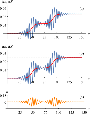
Figure 1: Numerical comparison of the particle and OC dynamics in a quasimonochromatic GW: blue – particle dynamics as predicted by Eqs. (11); red – the OC dynamics as predicted by Eqs. (75); black dashed – $\Delta\ell_{x}$ and $\Delta\ell_{\parallel}$ predicted by Eqs. (144). The GW propagates along the $z$ axis in vacuum with the Minkowski background metric. Spacetime scales are measured in units $\omega^{-1}$, so the GW wavevector is $k_{\alpha}=(-1,0,0,1)$. The perturbation metric is given by Eq. (131), with $h_{+}=h_{\times}=a(\theta)/2$, $a(\theta)=0.1[\mathrm{sech}(\epsilon\theta+13)-\mathrm{sech}(\epsilon\theta+7)]\sin{\theta}$, $\theta=k_{\alpha}x^{\alpha}$, and $\epsilon=0.1$ serves as the small GO parameter (Sec. III.1). The initial velocity is $u^{\alpha}(\tau=0)=(\sqrt{2},1,0,0)$. Shown are: (a) the transverse displacements relative to the unperturbed trajectory, $\Delta x(\tau)$ and $\Delta X[\mathcal{T}(\tau)]$; (b) the longitudinal displacements relative to the unperturbed trajectory, $\Delta z(\tau)$ and $\Delta Z[\mathcal{T}(\tau)]$; (c) the strength of the metric perturbation at the particle location, $a[\theta(\tau)]$. The function $\mathcal{T}(\tau)$ is calculated by numerical integration of Eq. (67), but in fact, the difference between $\mathcal{T}$ and $\tau$ is negligible for these figures.

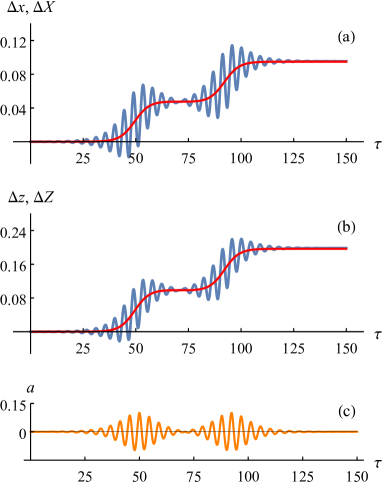
Figure 2: Same as Fig. 1 but for non-vacuum dispersion and polarization, namely, $k_{\alpha}=(-1,0,0,\sqrt{2})$ and $h_{\alpha\beta}=\delta_{\alpha\beta}a(\theta)/2$

.

VIII Conclusions

Here, we study the nonlinear secular dynamics of particles in prescribed quasimonochromatic GWs in a general background metric and for general GW dispersion and polarization. We show that this “ponderomotive” dynamics can be described by Hamilton’s equations (75), and we derive the corresponding Hamiltonian $\mathcal{H}$ to the second order in the GW amplitude. We find that $\mathcal{H}=\smash{H^{(0)}}+\smash{\mathcal{H}^{(2)}}$, where $\smash{H^{(0)}}$ is given by Eq. (72) and $\smash{\mathcal{H}^{(2)}}$ is given by Eq. (73), or equivalently, Eq. (96). For the special case of vacuum GWs, we show that our Hamiltonian $\mathcal{H}$ is equivalent to that of a free particle in an effective metric (126). We also show that already a linear plane GW pulse displaces a particle from its unperturbed trajectory by a finite distance that is independent of the GW phase and proportional to the integral of the pulse intensity. We calculate the particle displacement analytically [Eq. (144)] and show that our result is in agreement with numerical simulations of the particle motion in a prescribed metric. We also show how the Hamiltonian of the nonlinear averaged dynamics naturally leads to the concept of the linear gravitational susceptibility of a particle gas with an arbitrary phase-space distribution. This can be understood as a manifestation of the so-called $K$-$\chi$ theorem known from plasma physics. We calculate the gravitational susceptibility explicitly [Eq. (122)] to apply it, in a follow-up paper, toward studying self-consistent GWs in inhomogeneous media within the geometrical-optics approximation.

This material is based upon the work supported by National Science Foundation under the grant No. PHY 1903130.

Appendix A Field-theoretical calculation of the OC Hamiltonian

Here, we present a detailed field-theoretical derivation of the general OC Hamiltonian of a semiclassical particle that oscillates in a low-amplitude “modulating” wave. The calculation is similar to that in LABEL:my:lens (see also LABEL:my:qponder), but the starting point is somewhat different, so we shall restate the whole argument. Suppose a semiclassical particle with quantum phase $\vartheta$ and action density $\mathcal{I}$. Assume that the particle Lagrangian density $\mathfrak{L}$ is given by (86) and the Hamiltonian $H$ has the form

$$H(x,p)=\bar{H}(x,p)+\widetilde{H}(x,p),$$ (146)

$$\bar{H}(x,p)\doteq\langle H(x,p)\rangle_{\theta},\quad\langle\widetilde{H}(x,p)\rangle_{\theta}=0,$$ (147)

where $\widetilde{H}(x,p)=\widetilde{H}[\epsilon x,p,\theta(x)]$ is small (cf. Sec. III.1) and the average over the modulating-wave phase $\theta$ is taken at fixed momentum $p\doteq\nabla\vartheta$. (We assume units such that $\hbar=1$.) Using

$$\vartheta=\bar{\vartheta}+\widetilde{\vartheta},\quad\bar{\vartheta}\doteq\langle\vartheta\rangle_{\theta},$$ (148)

$$\mathcal{I}=\bar{\mathcal{I}}+\widetilde{\mathcal{I}},\quad\bar{\mathcal{I}}\doteq\langle\mathcal{I}\rangle_{\theta},$$ (149)

we obtain the following formula for $\mathfrak{L}$:

$$\mathfrak{L}=-(\bar{\mathcal{I}}+\tilde{\mathcal{I}})[\bar{H}(x,P+\widetilde{p})+\widetilde{H}(x,P+\widetilde{p})],$$ (150)

where $P\doteq\nabla\bar{\vartheta}$ and $\widetilde{p}\doteq\nabla\widetilde{\vartheta}$. Taylor-expanding $\bar{H}$ and $\widetilde{H}$ in $\widetilde{p}=O(\smash{\widetilde{H}})$ and neglecting terms of the third and higher orders in $\smash{\widetilde{H}}$, we obtain

$$\mathfrak{L}\simeq-\bar{\mathcal{I}}\,\bar{H}-\bar{\mathcal{I}}\,\frac{\partial\bar{H}}{\partial P_{\alpha}}\widetilde{p}_{\alpha}-\frac{\bar{\mathcal{I}}}{2}\frac{\partial^{2}\bar{H}}{\partial P_{\alpha}\partial P_{\beta}}\,\widetilde{p}_{\alpha}\widetilde{p}_{\beta}-\bar{\mathcal{I}}\,\widetilde{H}\\ -\bar{\mathcal{I}}\,\frac{\partial\widetilde{H}}{\partial P_{\alpha}}\,\widetilde{p}_{\alpha}-\widetilde{\mathcal{I}}\,\bar{H}-\widetilde{\mathcal{I}}\,\frac{\partial\bar{H}}{\partial P_{\alpha}}\widetilde{p}_{\alpha}-\widetilde{\mathcal{I}}\,\widetilde{H},$$ (151)

where all functions are evaluated at $(x,P)$. From the part of Eq. (87) that is linear in the the modulating-wave amplitude, one has

$$\widetilde{H}+\widetilde{p}_{\lambda}\mathsf{U}^{\lambda}=0,\quad\mathsf{U}^{\lambda}\doteq\partial\bar{H}/\partial P_{\lambda},$$ (152)

so the two last terms on the right-hand side on Eq. (151) mutually cancel out. [The definition of $\mathsf{U}^{\lambda}$ given here is in agreement with Eq. (94) within the assumed accuracy.] Then, the average Lagrangian density, $\bar{\mathfrak{L}}\doteq\langle\mathfrak{L}\rangle_{\theta}$, is given by $\bar{\mathfrak{L}}=-\bar{\mathcal{I}}\mathcal{H}$, where

$$\mathcal{H}=\bar{H}+\frac{1}{2}\frac{\partial^{2}\bar{H}}{\partial P_{\alpha}\partial P_{\beta}}\,\langle\widetilde{p}_{\alpha}\widetilde{p}_{\beta}\rangle_{\theta}+\bigg{\langle}\frac{\partial\widetilde{H}}{\partial P_{\alpha}}\,\widetilde{p}_{\alpha}\bigg{\rangle}_{\theta}.$$ (153)

Just like $H$ in Eq. (86) serves as a Hamiltonian for a particle, $\mathcal{H}$ serves as a Hamiltonian for the particle OC.

The oscillating part of the particle phase is quasiperiodic in $\theta$, so $\smash{\widetilde{\vartheta}}=\smash{\widetilde{\vartheta}}[\epsilon x,\theta(x)]$. Then, $\smash{\widetilde{p}_{\alpha}}\simeq k_{\alpha}\partial_{\theta}\smash{\widetilde{\vartheta}}$, where $k_{\alpha}\doteq\nabla_{\alpha}\theta$ is the wavevector of the modulating wave. Equation (152) gives $\partial_{\theta}\smash{\widetilde{\vartheta}}\simeq-\smash{\widetilde{H}/(k_{\lambda}\mathsf{U}^{\lambda})}$, so

$$\widetilde{p}_{\alpha}\simeq-\frac{k_{\alpha}\widetilde{H}}{k_{\lambda}\mathsf{U}^{\lambda}}.$$ (154)

By substituting this into Eq. (153), we then obtain

$$\mathcal{H} \simeq\bar{H}+\frac{\partial^{2}\bar{H}}{\partial P_{\alpha}\partial P_{\beta}}\,\frac{k_{\alpha}k_{\beta}\langle\widetilde{H}^{2}\rangle_{\theta}}{2(k_{\lambda}\mathsf{U}^{\lambda})^{2}}-\frac{k_{\alpha}}{k_{\lambda}\mathsf{U}^{\lambda}}\bigg{\langle}\frac{\partial\widetilde{H}}{\partial P_{\alpha}}\,\widetilde{H}\bigg{\rangle}_{\theta}$$

$$=\bar{H}+\frac{k_{\alpha}}{2}\bigg{[}k_{\beta}\,\frac{\partial\mathsf{U}^{\beta}}{\partial P_{\alpha}}\,\frac{\langle\widetilde{H}^{2}\rangle_{\theta}}{(k_{\lambda}\mathsf{U}^{\lambda})^{2}}-\frac{1}{k_{\lambda}\mathsf{U}^{\lambda}}\frac{\partial\langle\widetilde{H}^{2}\rangle_{\theta}}{\partial P_{\alpha}}\bigg{]}$$

$$=\bar{H}-\frac{k_{\alpha}}{2}\frac{\partial}{\partial P_{\alpha}}\bigg{(}\frac{\langle\widetilde{H}^{2}\rangle_{\theta}}{k_{\lambda}\mathsf{U}^{\lambda}}\bigg{)},$$ (155)

where we have used $\partial^{2}\bar{H}/\partial P_{\alpha}\partial P_{\beta}=\partial\mathsf{U}^{\beta}/\partial P_{\alpha}$. For $H$ of the form (89), this readily leads to Eq. (93).

Appendix B Derivation of the gravitational susceptibility

Here, we derive an explicit formula for the gravitational susceptibility $\mathcal{X}_{\alpha\beta\gamma\delta}$ of a particle gas from Eqs. (117) and (120). By combining the latter equations, one obtains

$$\mathcal{X}_{\alpha\beta\gamma\delta}=-\int\mathrm{d}{\boldsymbol{\rm P}}\,\frac{F}{4\mathsf{P}^{0}}\left[Q_{\alpha\beta\gamma\delta}-k_{\mu}\,\frac{\partial}{\partial P_{\mu}}\left(\frac{\mathscr{T}_{\alpha\beta}\mathscr{T}_{\gamma\delta}}{k^{\rho}P_{\rho}}\right)\right]_{P_{0}=\mathsf{P}_{0}}=(\mathcal{X}_{1}+\mathcal{X}_{2}+\mathcal{X}_{3})_{\alpha\beta\gamma\delta},$$ (156)

where we have introduced [assuming the parametrization $k_{\alpha}=(-\omega,{\boldsymbol{\rm k}})$]

$$(\mathcal{X}_{1})_{\alpha\beta\gamma\delta} \doteq-\int\mathrm{d}{\boldsymbol{\rm P}}\,\frac{F}{4\mathsf{P}^{0}}\,Q_{\alpha\beta\gamma\delta},$$ (157)

$$(\mathcal{X}_{2})_{\alpha\beta\gamma\delta} \doteq-\frac{\omega}{4}\int\mathrm{d}{\boldsymbol{\rm P}}\,\frac{F}{\mathsf{P}^{0}}\left[\frac{\partial}{\partial P_{0}}\left(\frac{\mathscr{T}_{\alpha\beta}\mathscr{T}_{\gamma\delta}}{k^{\rho}P_{\rho}}\right)\right]_{P_{0}=\mathsf{P}_{0}},$$ (158)

$$(\mathcal{X}_{3})_{\alpha\beta\gamma\delta} \doteq\frac{k_{a}}{4}\int\mathrm{d}{\boldsymbol{\rm P}}\,\frac{F}{\mathsf{P}^{0}}\left[\frac{\partial}{\partial P_{a}}\left(\frac{\mathscr{T}_{\alpha\beta}\mathscr{T}_{\gamma\delta}}{k^{\rho}P_{\rho}}\right)\right]_{P_{0}=\mathsf{P}_{0}}$$

$$=\frac{k_{a}}{4}\int\mathrm{d}^{4}P\,\delta(P_{0}-\mathsf{P}_{0})\,\frac{F}{\mathsf{P}^{0}}\frac{\partial}{\partial P_{a}}\left(\frac{\mathscr{T}_{\alpha\beta}\mathscr{T}_{\gamma\delta}}{k^{\rho}P_{\rho}}\right).$$ (159)

The latter equality permits taking the corresponding integral by parts. (Remember that the derivative $\partial/\partial P_{\mu}$ is taken at fixed $P_{\nu\neq\mu}$, which are independent only in the four-dimensional momentum space.) Specifically, one obtains

$$(\mathcal{X}_{3})_{\alpha\beta\gamma\delta} =-\frac{k_{a}}{4}\int\mathrm{d}^{4}P\,\delta^{\prime}(P_{0}-\mathsf{P}_{0})\left(-\frac{\partial\mathsf{P}_{0}}{\partial P_{a}}\right)\frac{F}{\mathsf{P}^{0}}\frac{\mathscr{T}_{\alpha\beta}\mathscr{T}_{\gamma\delta}}{k^{\rho}P_{\rho}}-\frac{k_{a}}{4}\int\mathrm{d}^{4}P\,\delta(P_{0}-\mathsf{P}_{0})\frac{\partial}{\partial P_{a}}\left(\frac{F}{\mathsf{P}^{0}}\right)\frac{\mathscr{T}_{\alpha\beta}\mathscr{T}_{\gamma\delta}}{k^{\rho}P_{\rho}}$$

$$\simeq-\frac{k_{a}}{4}\int\mathrm{d}^{4}P\,\delta^{\prime}(P_{0}-\mathsf{P}_{0})\frac{FV^{a}}{\mathsf{P}^{0}}\frac{\mathscr{T}_{\alpha\beta}\mathscr{T}_{\gamma\delta}}{k^{\rho}P_{\rho}}-\frac{k_{a}}{4}\int\mathrm{d}{\boldsymbol{\rm P}}\,\frac{\partial}{\partial P_{a}}\left(\frac{F}{\mathsf{P}^{0}}\right)\left(\frac{\mathscr{T}_{\alpha\beta}\mathscr{T}_{\gamma\delta}}{k^{\rho}P_{\rho}}\right)_{P_{0}=\mathsf{P}_{0}}$$

$$=\int\mathrm{d}^{4}P\,\delta(P_{0}-\mathsf{P}_{0})\,{\boldsymbol{\rm k}}\cdot{\boldsymbol{\rm V}}\,\frac{F}{4\mathsf{P}^{0}}\frac{\partial}{\partial P_{0}}\left(\frac{\mathscr{T}_{\alpha\beta}\mathscr{T}_{\gamma\delta}}{k^{\rho}P_{\rho}}\right)-\frac{k_{a}}{4}\int\frac{\mathrm{d}{\boldsymbol{\rm P}}}{\mathsf{P}^{0}}\left(\frac{\partial F}{\partial P_{a}}-\frac{F}{\mathsf{P}^{0}}\frac{\partial P^{0}}{\partial P_{a}}\right)\left(\frac{\mathscr{T}_{\alpha\beta}\mathscr{T}_{\gamma\delta}}{k^{\rho}P_{\rho}}\right)_{P_{0}=\mathsf{P}_{0}}$$

$$=\int\frac{\mathrm{d}{\boldsymbol{\rm P}}}{4\mathsf{P}^{0}}\left[({\boldsymbol{\rm k}}\cdot{\boldsymbol{\rm V}})F\,\frac{\partial}{\partial P_{0}}\left(\frac{\mathscr{T}_{\alpha\beta}\mathscr{T}_{\gamma\delta}}{k^{\rho}P_{\rho}}\right)-k_{a}\left(\frac{\partial F}{\partial P_{a}}-\frac{F}{\mathsf{P}^{0}}\frac{\partial P^{0}}{\partial P_{a}}\right)\left(\frac{\mathscr{T}_{\alpha\beta}\mathscr{T}_{\gamma\delta}}{k^{\rho}P_{\rho}}\right)\right]_{P_{0}=\mathsf{P}_{0}},$$ (160)

where we have used $-\partial\mathsf{P}_{0}/\partial P_{a}\simeq{\boldsymbol{\rm V}}$ [see Eqs. (81) and (83)]. Then, notice that

$$k^{\rho}P_{\rho}=k_{\rho}P^{\rho}=\mathsf{P}^{0}({\boldsymbol{\rm k}}\cdot{\boldsymbol{\rm V}}-\omega),$$ (161)

so the sum of Eqs. (158) and (160) can be written as follows:

$$(\mathcal{X}_{2}+\mathcal{X}_{3})_{\alpha\beta\gamma\delta}=\int\frac{\mathrm{d}{\boldsymbol{\rm P}}}{4\mathsf{P}^{0}}\bigg{\{}\frac{F}{\mathsf{P}^{0}}\left[k^{\rho}P_{\rho}\,\frac{\partial}{\partial P_{0}}\left(\frac{\mathscr{T}_{\alpha\beta}\mathscr{T}_{\gamma\delta}}{k^{\rho}P_{\rho}}\right)+k^{0}\frac{\mathscr{T}_{\alpha\beta}\mathscr{T}_{\gamma\delta}}{k^{\rho}P_{\rho}}\right]-\left(k_{a}\,\frac{\partial F}{\partial P_{a}}-\frac{F}{\mathsf{P}^{0}}\,k_{a}\frac{\partial P^{0}}{\partial P_{a}}\right)\left(\frac{\mathscr{T}_{\alpha\beta}\mathscr{T}_{\gamma\delta}}{k^{\rho}P_{\rho}}\right)\bigg{\}}_{P_{0}=\mathsf{P}_{0}}.$$

Notice that $\partial(k^{\rho}P_{\rho})/\partial P_{0}=k^{0}$, so the whole expression in the square brackets is simply $\partial(\mathscr{T}_{\alpha\beta}\mathscr{T}_{\gamma\delta})/\partial P_{0}$. Also,

$$\frac{\partial\mathsf{P}^{0}}{\partial P_{a}}=\frac{\partial}{\partial P_{a}}\,(\bar{g}^{00}\mathsf{P}_{0}+\bar{g}^{0b}P_{b})=\bar{g}^{00}\,\frac{\partial\mathsf{P}_{0}}{\partial P_{a}}+\bar{g}^{0a}\simeq\bar{g}^{0a}-\bar{g}^{00}V^{a},$$ (162)

$$k_{a}\,\frac{\partial\mathsf{P}^{0}}{\partial P_{a}}=\bar{g}^{0a}k_{a}-\bar{g}^{00}k_{a}V^{a}=k^{0}-\bar{g}^{00}k_{0}-\bar{g}^{00}k_{a}V^{a}=k^{0}+\bar{g}^{00}(\omega-{\boldsymbol{\rm k}}\cdot{\boldsymbol{\rm V}})=k^{0}-\frac{\bar{g}^{00}}{\mathsf{P}^{0}}\,k^{\rho}P_{\rho}.$$ (163)

Then, the above equation can be written as follows:

$$(\mathcal{X}_{2}+\mathcal{X}_{3})_{\alpha\beta\gamma\delta} =\int\frac{\mathrm{d}{\boldsymbol{\rm P}}}{4\mathsf{P}^{0}}\bigg{[}\frac{F}{\mathsf{P}^{0}}\,\frac{\partial(\mathscr{T}_{\alpha\beta}\mathscr{T}_{\gamma\delta})}{\partial P_{0}}-\left(k_{a}\,\frac{\partial F}{\partial P_{a}}+\bar{g}^{00}k^{\rho}P_{\rho}\,\frac{F}{(\mathsf{P}^{0})^{2}}\right)\left(\frac{\mathscr{T}_{\alpha\beta}\mathscr{T}_{\gamma\delta}}{k^{\rho}P_{\rho}}\right)\bigg{]}_{P_{0}=\mathsf{P}_{0}}$$

$$=\int\frac{\mathrm{d}{\boldsymbol{\rm P}}}{4(\mathsf{P}^{0})^{2}}\,\frac{{\boldsymbol{\rm k}}\cdot\partial_{\boldsymbol{\rm P}}F}{\omega-{\boldsymbol{\rm k}}\cdot{\boldsymbol{\rm V}}}\,(\mathscr{T}_{\alpha\beta}\mathscr{T}_{\gamma\delta})_{P_{0}=\mathsf{P}_{0}}+\int\frac{\mathrm{d}{\boldsymbol{\rm P}}}{4(\mathsf{P}^{0})^{2}}\,F\bigg{[}\frac{\partial(\mathscr{T}_{\alpha\beta}\mathscr{T}_{\gamma\delta})}{\partial P_{0}}-\frac{\bar{g}^{00}}{\mathsf{P}^{0}}\,\mathscr{T}_{\alpha\beta}\mathscr{T}_{\gamma\delta}\bigg{]}_{P_{0}=\mathsf{P}_{0}}.$$ (164)

Together with Eqs. (156) and (157), this leads to

$$\mathcal{X}_{\alpha\beta\gamma\delta}=\int\frac{\mathrm{d}{\boldsymbol{\rm P}}}{4(\mathsf{P}^{0})^{2}}\left\{\frac{{\boldsymbol{\rm k}}\cdot\partial_{\boldsymbol{\rm P}}F}{\omega-{\boldsymbol{\rm k}}\cdot{\boldsymbol{\rm V}}}\,\mathscr{T}_{\alpha\beta}\mathscr{T}_{\gamma\delta}+FJ_{\alpha\beta\gamma\delta}\bigg{]}\right\}_{P_{0}=\mathsf{P}_{0}},$$ (165)

where

$$J_{\alpha\beta\gamma\delta}\doteq\frac{\partial(\mathscr{T}_{\alpha\beta}\mathscr{T}_{\gamma\delta})}{\partial P_{0}}-\frac{\bar{g}^{00}}{\mathsf{P}^{0}}\,\mathscr{T}_{\alpha\beta}\mathscr{T}_{\gamma\delta}-\mathsf{P}^{0}Q_{\alpha\beta\gamma\delta}=\frac{\partial(\mathscr{T}_{\alpha\beta}\mathscr{T}_{\gamma\delta})}{\partial P_{0}}-(\mathsf{P}^{0})^{2}\left(\frac{\mathscr{T}_{\alpha\beta}\mathscr{T}_{\gamma\delta}}{m^{2}+\bar{\sigma}^{ab}P_{a}P_{b}}+Q_{\alpha\beta\gamma\delta}\right).$$ (166)

Here, the tensor $\bar{\sigma}^{ab}\doteq\bar{g}^{ab}-\bar{g}^{a0}\bar{g}^{b0}/\bar{g}^{00}$ (same as in Sec. IV.3) is introduced by analogy with $\sigma^{ab}$ in Eq. (18), and one can further substitute

$$\frac{\partial(\mathscr{T}_{\alpha\beta}\mathscr{T}_{\gamma\delta})}{\partial P_{0}}=\delta_{\alpha}^{0}P_{\beta}P_{\gamma}P_{\delta}+P_{\alpha}\delta_{\beta}^{0}P_{\gamma}P_{\delta}+P_{\alpha}P_{\beta}\delta^{0}_{\gamma}P_{\delta}+P_{\alpha}P_{\beta}P_{\gamma}\delta^{0}_{\delta}.$$ (167)

References

• (1) B. P. Abbott et al., Observation of gravitational waves from a binary black hole merger, Phys. Rev. Lett. 116, 061102 (2016).
• (2) B. P. Abbott et al., GW151226: Observation of gravitational waves from a 22-solar-mass binary black hole coalescence, Phys. Rev. Lett. 116, 241103 (2016).
• (3) B. P. Abbott et al., GW170104: Observation of a 50-solar-mass binary black hole coalescence at redshift 0.2, Phys. Rev. Lett. 118, 221101 (2017).
• (4) B. P. Abbott et al., GW170608: Observation of a 19 solar-mass binary black hole coalescence, Astrophys. J. Lett. 851, L35 (2017).
• (5) B. P. Abbott et al., GW170814: A three-detector observation of gravitational waves from a binary black hole coalescence, Phys. Rev. Lett. 119, 141101 (2017).
• (6) B. P. Abbott et al., GW170817: Observation of gravitational waves from a binary neutron star inspiral, Phys. Rev. Lett. 119, 161101 (2017).
• (7) B. P. Abbott et al., GWTC-1: A gravitational-wave transient catalog of compact binary mergers observed by LIGO and Virgo during the first and second observing runs, Phys. Rev. X 9, 031040 (2019).
• (8) B. P. Abbott et al., GW190425: Observation of a compact binary coalescence with total mass $\sim$ 3.4 $M_{\odot}$, Astrophys. J. Lett. 892, L3 (2020).
• (9) B. P. Abbott et al., GW190412: Observation of a binary-black-hole coalescence with asymmetric masses, arXiv:2004.08342.
• (10) Ya. B. Zel’dovich and A. G. Polnarev, Radiation of gravitational waves by a cluster of superdense stars, Astron. Zh. 51, 30 (1974) [Sov. Astron. 18, 17 (1974)].
• (11) V. B. Braginskii and L. P. Grishchuk, Kinematic resonance and memory effect in free-mass gravitational antennas, Zh. Eksp. Teor. Fiz. 89, 744 (1985) [Sov. Phys. JETP 62, 427 (1985)].
• (12) V. B. Braginsky and K. S. Thorne, Gravitational-wave bursts with memory and experimental prospects, Nature 327, 123 (1987).
• (13) D. Chesters, Dispersion of gravitational waves by a collisionless gas, Phys. Rev. D 7, 2863 (1973).
• (14) E. Asseo, D. Gerbal, J. Heyvaerts, and M. Signore, General-relativistic kinetic theory of waves in a massive particle medium, Phys. Rev. D 13, 2724 (1976).
• (15) P. G. Macedo and A. H. Nelson, Propagation of gravitational waves in a magnetized plasma, Phys. Rev. D 28, 2382 (1983).
• (16) M. Servin, G. Brodin, and M. Marklund, Cyclotron damping and Faraday rotation of gravitational waves, Phys. Rev. D 64, 024013 (2001).
• (17) J. Moortgat and J. Kuijpers, Gravitational and magnetosonic waves in gamma-ray bursts, Astron. Astrophys. 402, 905 (2003).
• (18) M. Forsberg and G. Brodin, Linear theory of gravitational wave propagation in a magnetized, relativistic Vlasov plasma, Phys. Rev. D 82, 124029 (2010).
• (19) D. Barta and M. Vasúth, Dispersion of gravitational waves in cold spherical interstellar medium, Int. J. Mod. Phys. D 27, 1850040 (2018).
• (20) L. Blanchet and T. Damour, Hereditary effects in gravitational radiation, Phys. Rev. D 46, 4304 (1992).
• (21) D. Christodoulou, Nonlinear nature of gravitation and gravitational-wave experiments, Phys. Rev. Lett. 67, 1486 (1991).
• (22) K. S. Thorne, Gravitational-wave bursts with memory: The Christodoulou effect, Phys. Rev. D 45, 520 (1992).
• (23) A. G. Wiseman and C. M. Will, Christodoulou’s nonlinear gravitational-wave memory: Evaluation in the quadrupole approximation, Phys. Rev. D 44, R2945 (1991).
• (24) P.-M. Zhang, C. Duval, G. W. Gibbons, and P.A. Horvathy, Velocity memory effect for polarized gravitational waves, J. Cosmol. Astropart. Phys. 5, 30 (2018).
• (25) P.-M. Zhang, C. Duval, G. W. Gibbons, P. A. Horvathy, The memory effect for plane gravitational waves, Phys. Lett. B 772, 743 (2017).
• (26) É. É. Flanagan, A. M. Grant, A. I. Harte, and D. A. Nichols, Persistent gravitational wave observables: General framework, Phys. Rev. D 99, 084044 (2019).
• (27) A. G. Wiseman, Coalescing binary systems of compact objects to (post)5/2-Newtonian order. IV. The gravitational wave tail, Phys. Rev. D 48, 4757 (1993).
• (28) Y. G. Ignat’ev, Gravitational magnetic shocks as a detector of gravitational waves, Phys. Lett. A 230, 171 (1997).
• (29) G. Brodin and M. Marklund, Parametric excitation of plasma waves by gravitational radiation, Phys. Rev. Lett. 82, 3012 (1999).
• (30) G. Brodin, M. Marklund, and P. K. S. Dunsby, Nonlinear gravitational wave interactions with plasmas, Phys. Rev. D 62, 104008 (2000).
• (31) M. Servin, G. Brodin, M. Bradley, and M. Marklund, Parametric excitation of Alfvén waves by gravitational radiation, Phys. Rev. E 62, 8493 (2000).
• (32) D. Papadopoulos, N. Stergioulas, L. Vlahos, and J. Kuijpers, Fast magnetosonic waves driven by gravitational waves, Astron. Astrophys. 377, 701 (2001).
• (33) G. Brodin, M. Marklund, and M. Servin, Photon frequency conversion induced by gravitational radiation, Phys. Rev. D 63, 124003 (2001).
• (34) A. B. Balakin, V. R. Kurbanova, and W. Zimdahl, Parametric phenomena of the particle dynamics in a periodic gravitational wave field, J. Math. Phys. 44, 5120 (2003).
• (35) M. Servin and G. Brodin, Resonant interaction between gravitational waves, electromagnetic waves, and plasma flows, Phys. Rev. D 68, 044017 (2003).
• (36) A. Källberg, G. Brodin, and M. Bradley, Nonlinear coupled Alfvén and gravitational waves, Phys. Rev. D 70, 044014 (2004).
• (37) L. Vlahos, G. Voyatzis, and D. Papadopoulos, Impulsive electron acceleration by gravitational waves, Astrophys. J. 604, 297 (2004).
• (38) G. Brodin, M. Marklund, and P. K. Shukla, Generation of gravitational radiation in dusty plasmas and supernovae, J. Exp. Theor. Phys. 81, 135 (2005).
• (39) M. D. Duez, Y. T. Liu, S. L. Shapiro, and B. C. Stephens, Relativistic magnetohydrodynamics in dynamical spacetimes: Numerical methods and tests, Phys. Rev. D 72, 024028 (2005).
• (40) H. Isliker, I. Sandberg, and L. Vlahos, Interaction of gravitational waves with strongly magnetized plasmas, Phys. Rev. D 74, 104009 (2006).
• (41) M. Forsberg, G. Brodin, M. Marklund, P. K. Shukla, and J. Moortgat, Nonlinear interactions between gravitational radiation and modified Alfvén modes in astrophysical dusty plasmas, Phys. Rev. D 74, 064014 (2006).
• (42) B. D. Farris, T. K. Li, Y. T. Liu, and S. L. Shapiro, Relativistic radiation magnetohydrodynamics in dynamical spacetimes: Numerical methods and tests, Phys. Rev. D 78, 024023 (2008).
• (43) M. Forsberg and G. Brodin, Harmonic generation of gravitational wave induced Alfvén waves, Phys. Rev. D 77, 024050 (2008).
• (44) G. Brodin, M. Forsberg, M. Marklund, and D. Eriksson, Interaction between gravitational waves and plasma waves in the Vlasov description, J. Plasma Phys. 76, 345 (2010).
• (45) A. V. Gaponov and M. A. Miller, Potential wells for charged particles in a high-frequency electromagnetic field, Zh. Eksp. Teor. Fiz. 34, 242 (1958) [Sov. Phys. JETP 7, 168 (1958)].
• (46) H. Motz and C. J. H. Watson, The radio-frequency confinement and acceleration of plasmas, Adv. Electron. Electron Phys. 23, 153 (1967).
• (47) J. R. Cary and A. N. Kaufman, Ponderomotive effects in collisionless plasma: a Lie transform approach, Phys. Fluids 24, 1238 (1981).
• (48) I. Y. Dodin and N. J. Fisch, Positive and negative effective mass of classical particles in oscillatory and static fields, Phys. Rev. E 77, 036402 (2008).
• (49) D. E. Ruiz, C. L. Ellison, and I. Y. Dodin, Relativistic ponderomotive Hamiltonian of a Dirac particle in a vacuum laser field, Phys. Rev. A 92, 062124 (2015).
• (50) J. R. Cary and A. N. Kaufman, Ponderomotive force and linear susceptibility in Vlasov plasma, Phys. Rev. Lett. 39, 402 (1977).
• (51) A. N. Kaufman, Phase-space-Lagrangian action principle and the generalized $K$-$\chi$ theorem, Phys. Rev. A 36, 982 (1987).
• (52) G. W. Kentwell, Oscillation-center theory at resonance, Phys. Rev. A 35, 4703 (1987).
• (53) I. Y. Dodin and N. J. Fisch, On generalizing the $K$-$\chi$ theorem, Phys. Lett. A 374, 3472 (2010).
• (54) I. Y. Dodin and N. J. Fisch, Ponderomotive forces on waves in modulated media, Phys. Rev. Lett. 112, 205002 (2014).
• (55) D. E. Ruiz and I. Y. Dodin, Ponderomotive dynamics of waves in quasiperiodically modulated media, Phys. Rev. A 95, 032114 (2017).
• (56) I. Y. Dodin, On variational methods in the physics of plasma waves, Fusion Sci. Tech. 65, 54 (2014).
• (57) I. Y. Dodin and N. J. Fisch, Nonlinear dispersion of stationary waves in collisionless plasmas, Phys. Rev. Lett. 107, 035005 (2011).
• (58) I. Y. Dodin and N. J. Fisch, Adiabatic nonlinear waves with trapped particles: I. General formalism, Phys. Plasmas 19, 012102 (2012).
• (59) C. Liu and I. Y. Dodin, Nonlinear frequency shift of electrostatic waves in general collisionless plasma: unifying theory of fluid and kinetic nonlinearities, Phys. Plasmas 22, 082117 (2015).
• (60) L. D. Landau and E. M. Lifshitz, The Classical Theory of Fields (Pergamon Press, New York, 1971).
• (61) G. Cognola, L. Vanzo, and S. Zerbini, Relativistic wave mechanics of spinless particles in a curved space-time, Gen. Relativ. Gravit. 18, 971 (1986).
• (62) See Supplemental Material in I. Y. Dodin and N. J. Fisch, Vlasov equation and collisionless hydrodynamics adapted to curved spacetime, Phys. Plasmas 17, 112118 (2010).
• (63) A. J. Brizard, Variational principles for reduced plasma physics, J. Phys. Conf. Ser. 169, 012003 (2009).
• (64) L. D. Landau and E. M. Lifshitz, Mechanics (Butterworth-Heinemann, Oxford, 1976).
• (65) E. R. Tracy, A. J. Brizard, A. S. Richardson, and A. N. Kaufman, Ray Tracing and Beyond: Phase Space Methods in Plasma Wave Theory (Cambridge University Press, New York, 2014).
• (66) I. Y. Dodin and N. J. Fisch, Axiomatic geometrical optics, Abraham-Minkowski controversy, and photon properties derived classically, Phys. Rev. A 86, 053834 (2012).
• (67) I. Y. Dodin, Geometric view on noneikonal waves, Phys. Lett. A 378, 1598 (2014).
• (68) B. S. DeWitt, Point transformations in quantum mechanics, Phys. Rev. 85, 653 (1952).
• (69) D. E. Ruiz and I. Y. Dodin, On the correspondence between quantum and classical variational principles, Phys. Lett. A 379, 2623 (2015).
• (70) I. Y. Dodin, A. I. Zhmoginov, and D. E. Ruiz, Variational principles for dissipative (sub)systems, with applications to the theory of linear dispersion and geometrical optics, Phys. Lett. A 381, 1411 (2017).
• (71) T. H. Stix, Waves in Plasmas (AIP, New York, 1992).
• (72) S. A. Trigger, A. I. Ershkovich, G. J. F. van Heijst, and P. P. J. M. Schram, Kinetic theory of Jeans instability, Phys. Rev. E 69, 066403 (2004).
• (73) A. I. Harte, Optics in a nonlinear gravitational plane wave, Classical Quant. Grav. 32, 175017 (2015).
• (74) I. Y. Dodin and N. J. Fisch, Relativistic electron acceleration in focused laser fields after above-threshold ionization, Phys. Rev. E 68, 056402 (2003).
• (75) D. L. Bruhwiler and J. R. Cary, Particle dynamics in a large-amplitude wave packet, Phys. Rev. Lett. 68, 255 (1992).
• (76) D. L. Bruhwiler and J. R. Cary, Dynamics of particle trapping and detrapping in coherent wave packets, Phys. Rev. E 50, 3949 (1994).
• (77) B. Schutz, A First Course in General Relativity (Cambridge University Press, New York, 2009), p. 206.