Morse potential in relativistic contexts from generalized momentum operator, Pekeris approximation revisited and mapping

Abstract

In this work we explore a generalization of the Dirac and Klein-Gordon (KG) oscillators, provided with a deformed linear momentum inspired in nonextensive statistics, that gives place to the Morse potential in relativistic contexts by first principles. In the (1+1)–dimensional case the relativistic oscillators are mapped into the quantum Morse potential. Using the Pekeris approximation, in the (3+1)–dimensional case we study the thermodynamics of the S-waves states ($l=0$) of the H₂, LiH, HCl and CO molecules (in the non-relativistic limit) and of a relativistic electron, where Schottky anomalies (due to the finiteness of the Morse spectrum) and spin contributions to the heat capacity are reported. By revisiting a generalized Pekeris approximation, we provide a mapping from (3+1)–dimensional Dirac and KG equations with a spherical potential to an associated one-dimensional Schrödinger-like equation, and we obtain the family of potentials for which this mapping corresponds to a Schrödinger equation with non-minimal coupling.

1 Introduction

For compatibilizing the principles of quantum mechanics with the special relativity, the Klein-Gordon (KG) and the Dirac equations constitute the two most relevant cases that were found, both satisfying the quadratic relativistic relation $E^{2}=p^{2}c^{2}+m^{2}c^{4}$. The KG equation is obtained by means of the quantization this relation, which leads to a relativistic wave equation with second order derivatives in time and space that is Lorentz-covariant, while Dirac focused on a relativistic first order wave equation describing the behavior of electrons consistently with the special relativity [1].

In Refs. [2, 3, 4] an harmonic potential has been incorporated by adding to the linear momentum (non-minimum coupling) a linear function, thus obtaining the so called Dirac and KG oscillators, that in the non-relativistic limit gives the quantum harmonic oscillator for spinless and strong spin-orbit coupling fermionic particles. These types of linear interactions were employed in quarks mass spectra [5], on a Coulomb-like potential [6, 7], in $2D$ massless fermions [8] and propagators [9], in curved space-time [10], in systems with extended and generalized uncertainty principle [11, 12]. Also, the non-relativistic quantum-mechanical formalism was studied by some authors [13, 14, 15], that have considered the harmonic oscillator provided with a generalized linear momentum operator which allows to obtain the Morse potential [16] by first principles. Recently, some of us have characterized a deformed lattice using the same generalized linear momentum operator [17].

The goal of this letter is twofold. First, we extend the strategy used in [14] to the one-dimensional and three-dimensional KG and Dirac oscillators in order to obtain the corresponding relativistic equations for a Morse potential coupling [18, 19, 20, 21, 22, 23, 24, 25, 26, 27, 28, 29, 30, 31, 32, 33]. Then, from a generalized Pekeris approximation we obtain a mapping between (3+1)-dimensional KG and Dirac equations and Schrödinger-like ones for arbitrary spherical potentials. The work begins with the preliminaries, with the development of a generalized linear momentum operator formulation in the Hamiltonian, showing that both oscillators with this coupling are equivalent the one-dimensional KG and Dirac particles provided with a Morse potential coupling and the standard linear momentum. We illustrate the results with those obtained in the literature for the $\textrm{H}_{2}$ molecule [34, 35, 36]. Using the Pekeris approximation [37] in the three-dimensional case for the Morse potential non-minimal coupling, we obtain the eigenvalues and the eigenfunctions, and then we recover the non-relativistic and the non-deformed limits for both cases. Hence, in order to test our approximations in the three-dimensional case, we study the thermodynamics of the S-wave states ($l=0$) for the H₂, LiH, HCL and CO molecules (in the non-relativistic limit) and of an electron in the high energy relativistic regime. Here, Schottky anomalies are reported in the heat capacity as a consequence of the spectrum finiteness of the Morse potential mapping. Next, we revisit the generalized Pekeris approximation [38] to provide a mapping for passing from (3+1)-dimensional KG and Dirac equations with an arbitrary spherical non-minimal coupling to an associated Schrödinger-like equation. Also, we determine the family of potential couplings from which the mapping is performed onto a Schrödinger equation with non-minimal coupling. Finally, we outline our conclusions.

2 Preliminaries

We present the preliminaries used throughout the work.

2.1 Morse potential and generalized momentum operator

Some authors [13, 14, 15, 39, 40, 41, 17] have investigated a generalized translation operator that gives a nonadditive spatial displacement of the form

$$\hat{\mathcal{T}}_{\gamma}(\varepsilon)|x\rangle=|x+\varepsilon+\gamma x\varepsilon\rangle$$ (1)

being $\varepsilon$ an infinitesimal displacement and $\gamma$ a parameter with dimension of inverse length in such a way that $\gamma_{q}\equiv(1-q)/\xi$ (from now on we place implicitly the dependence on $q$ in $\gamma$) with $\xi$ the characteristic length of the system, where the usual translation is recovered for $q\rightarrow 1$ ($\gamma\rightarrow 0$). These investigations were inspired by the development of Tsallis nonextensive thermostatistics [42, 43, 44] along with some of its mathematical implications (the $q$-calculus [45]). In Ref. [13, 14, 15] by means of $\hat{\mathcal{T}}_{\gamma}(\varepsilon)$ the authors obtained the generalized momentum operator $\hat{p}_{\gamma}|\alpha\rangle=-i\hbar D_{\gamma}|\alpha\rangle$ in the basis $x$, being $D_{\gamma}$ the deformed derivative in $x$

$$D_{\gamma}=(1+\gamma x)\frac{d}{dx}.$$ (2)

By means of the Hamiltonian $H=\hat{p}_{\gamma}^{2}+V(x)$ and using (2) it follows the (deformed) Schrödinger-like equation

$$i\hbar\frac{\partial}{\partial t}\psi(x,t)=-\frac{\hbar^{2}}{2m}D_{\gamma}^{2}\psi(x,t)+V(x)\psi(x,t)$$ (3)

that corresponds to a particle provided with an effective mass $m(x)=m/(1+\gamma x)^{2}$. Eq. (3) has been employed in applications of semiconductor heterostructures [46, 47].

An interesting application of the deformed Schrödinger equation (3) was given in order to derive the Morse potential by using first principles [14]. More precisely, by considering the coordinate transformation

$$\eta=\frac{\ln(1+\gamma x)}{\gamma}$$ (4)

in (3) along with the harmonic potential $V(x)=m\omega^{2}x^{2}/2$ and $\phi(\eta,t)=\psi(x(\eta),t)$ the following equation is obtained (using $E=i\hbar\frac{\partial}{\partial t}$)

$$E\phi(\eta,t)=-\frac{\hbar^{2}}{2m}\frac{d^{2}}{d\eta^{2}}\phi(\eta,t)+\frac{m\omega^{2}}{2\gamma^{2}}(e^{\gamma\eta}-1)^{2}\phi(\eta,t),$$ (5)

which is precisely the eigenvalues equation of the quantum Morse oscillator (QMO) [16]. This is provided of an effective potential $V_{\textrm{eff}}(\eta)=D(e^{\gamma\eta}-1)^{2}$, for the wave function $\phi(\eta,t)$ in the $\eta$ space with the dissociation parameter $D=\frac{m\omega^{2}}{2\gamma^{2}}$. The eigenfunctions of the QMO are given by

$$\Phi_{n}(z)=A_{n}z^{s}e^{-\frac{1}{2}z}L_{n}^{2s}(z)$$ (6)

with $A_{n}$ the normalization constant, $z=2m\omega e^{\gamma\eta}/(\gamma^{2}\hbar)$, $s=m\omega/(\gamma^{2}\hbar)-n-1/2$ and $L_{n}^{2s}(z)=(z^{-2s}e^{z}/n!)d^{n}(e^{-z}z^{n+2s})/dz^{n}$ the generalized Laguerre polynomial [48]. The energy spectrum of the QMO is

$$E_{n}=\hbar\omega\left(n+\frac{1}{2}\right)\left[1-\frac{\gamma^{2}\hbar}{2m\omega}\left(n+\frac{1}{2}\right)\right]$$ (7)

being $n$ restricted to the range $0\leq 2n\leq 2m\omega/(\gamma^{2}\hbar)-1$, which implies a finite number of states and $E_{n}\geq\hbar\omega(n+1/2)/2$. From (7) it can be seen that the harmonic oscillator energies are recovered for $\gamma\rightarrow 0$.

2.2 Klein-Gordon and Dirac oscillators

The substitution of the four-vector energy-momentum $\mathbf{p}^{\mu}=(E/c,\textbf{p})=(i\hbar\partial/\partial t,-i\hbar\nabla)$ in the quadratic relativistic relation for the case of an harmonic coupling prescription gives the Klein-Gordon oscillator [3, 4]

$$2m\mathcal{E}\psi=(\textbf{p}+im\omega\textbf{r})\cdot(\textbf{p}-im\omega\textbf{r})\psi,$$ (8)

where the form $(\textbf{p}+im\omega\textbf{r})\cdot(\textbf{p}-im\omega\textbf{r})$ ensures the Hermiticity [49]. From now on, for practical and notation reasons we will denote $\mathcal{E}$ as $\frac{E^{2}-m^{2}c^{4}}{2mc^{2}}$ with $E$ the energy of the particle. Here $\omega$ is the frequency of the oscillator, $m$ the mass and r the position, with the limit $\omega\rightarrow 0$ the corresponding one to the free particle case. Using algebraic methods the energies $E_{N}$ for the one-dimensional case result [49]

$$\mathcal{E}_{N}=N\hbar\omega\quad,\quad N=0,1,2,\ldots$$ (9)

with $\mathcal{E}_{N}=(E_{N}^{2}-m^{2}c^{4})/2mc^{2}$. In the non-relativistic limit $E=mc^{2}+\epsilon$ with $\epsilon\ll mc^{2}$ and then we have $\epsilon_{N}\approx N\hbar\omega$ ($N=0,1,2,\ldots$) that correspond to the energies of the harmonic oscillator provided with a zero ground state energy.

The usual form of the Dirac equation for a particle of mass $m$ is given by

$$\left[i\hbar\beta\frac{\partial}{\partial t}+i\hbar\beta\overrightarrow{\alpha}\cdot\overrightarrow{\nabla}-\frac{mc}{\hbar}\right]\psi=0$$ (10)

where $\beta$ and $\overrightarrow{\alpha}$ provide the $(3+1)$ representation of the Dirac matrices

$$\beta=\begin{pmatrix}\mathbf{I}&0\\ 0&-\mathbf{I}\end{pmatrix};\hskip 14.22636pt\alpha^{i}=\begin{pmatrix}0&\sigma^{i}\\ \sigma^{i}&0\end{pmatrix};$$

and $\mathbf{I}$ is the $2\times 2$ identity with $\sigma^{1},\sigma^{2}$ and $\sigma^{3}$ the $2\times 2$ Pauli matrices. Using the non-minimal harmonic coupling $\textbf{p}-im\beta\omega\textbf{r}$ in (10) we obtain the Dirac oscillator [2]

$$(E-mc^{2})\psi_{1}=c\overrightarrow{\sigma}\cdot(\textbf{p}+im\omega\textbf{r})\psi_{2}$$

$$(E+mc^{2})\psi_{2}=c\overrightarrow{\sigma}\cdot(\textbf{p}-im\omega\textbf{r})\psi_{1}$$ (11)

where $\omega$ is the frequency of the oscillator and $\psi^{T}=(\psi_{1},\psi_{2})$ is the spinorial wavefunction. From (2.2) it follows the differential equation for $\psi_{1}$

$$\mathcal{E}\psi_{1}=\left[\frac{p^{2}}{2m}+\frac{m\omega^{2}r^{2}}{2}-\frac{3}{2}\hbar\omega-\frac{2\omega}{\hbar}\mathbf{L}\cdot\mathbf{S}\right]\psi_{1}$$ (12)

where $\mathbf{L}=\mathbf{r}\times\mathbf{p}$ is the angular momentum and $\mathbf{S}=(\hbar/2)\sigma$ is the spin operator. By means of the total spin $\mathbf{J}=\mathbf{L}+\mathbf{S}$ it can be shown that the energies $E_{Nlj}$ are [2]

$$E_{Nlj}^{2}-m^{2}c^{4}=\hbar\omega[2(N+1-j)\mp 1]mc^{2},$$ (13)

$$\hskip 113.81102pt\quad\textrm{if}\quad l=j\mp\frac{1}{2}$$

which presents a degeneracy (typically of central potentials) for the pairs $(N\pm 1,j\mp 1),(N\pm 2,j\mp 2),\ldots$. From (13) in the non-relativistic limit $E=mc^{2}+\epsilon$ with $\epsilon\ll mc^{2}$ we have $\mathcal{E}=\epsilon_{Nlj}\approx\hbar\omega(N+1-j\mp\frac{1}{2})$ for $N=0,1,2,\ldots$ and $l=j\mp\frac{1}{2}$, so we recover the energies of the harmonic oscillator energies plus a strong spin-orbit term.

3 Morse potential for Klein-Gordon and Dirac equations from generalized momentum couplings

We present the Klein-Gordon and Dirac equations with Morse potential from the Klein-Gordon and Dirac oscillators provided with a generalized momentum coupling. We consider the one-dimensional and the three-dimensional cases.

3.1 One-dimensional case

Considering the Eq. (8) in one dimension with the deformed derivative (2) we have

$$2m\mathcal{E}\psi(x)=(p_{\gamma}+im\omega x)(p_{\gamma}-im\omega x)\psi(x),$$ (14)

that can be considered the Klein-Gordon version of the generalized harmonic oscillator studied in [13, 14]. From (14) and using the coordinate transformation (4) we have

$$\mathcal{E}\phi(\eta)=\frac{1}{2m}\Bigg{\{}\left[-i\hbar\frac{d}{d\eta}+im\omega\left(\frac{e^{\gamma\eta}-1}{\gamma}\right)\right]\times$$

$$\left[-i\hbar\frac{d}{d\eta}-im\omega\left(\frac{e^{\gamma\eta}-1}{\gamma}\right)\right]\Bigg{\}}\phi(\eta)$$ (15)

which corresponds to the Klein-Gordon equation with the non-minimal coupling $p_{\gamma}-im\omega(e^{\gamma\eta}-1)/\gamma$ for relativistic wave-function $\phi(\eta,t)=\psi(x(\eta),t)$ in the $\eta$-space. It is worthing to note that Eqns. (14) and (3.1) extend the equivalence between the harmonic oscillator with the generalized momentum $p_{\gamma}$ and the Morse potential [14], in the context of the KG equation. Moreover, by redefining $\eta$ as $\widetilde{\eta}=\eta-\eta_{0}$ and $\phi(\eta)$ as $\widetilde{\phi}(\widetilde{\eta})=\phi(\widetilde{\eta}+\eta_{0})$ the (3.1) can be rewritten as

$$\mathcal{E}\widetilde{\phi}(\widetilde{\eta})=\left[-\frac{\hbar^{2}}{2m}\frac{d^{2}}{d\widetilde{\eta}^{2}}+\frac{m\widetilde{\omega}^{2}}{2\gamma^{2}}(e^{\gamma\widetilde{\eta}}-1)^{2}-\frac{\hbar\widetilde{\omega}}{2}\right]\widetilde{\phi}(\widetilde{\eta})$$ (16)

where $\eta_{0}=\frac{\ln(\widetilde{\omega}/\omega)}{\gamma}$ and $\widetilde{\omega}=\omega\left(1+\frac{\gamma^{2}\hbar}{2m\omega}\right)$ is a modified frequency with $\eta_{0}$ a displacement of the origin of the potential, both arising due to the relativistic coupling. By comparison between the Eqns. (5)–(7) and the Eq. (16) it is obtained the energy spectrum of the KGMO (Klein-Gordon Morse oscillator)

$$\mathcal{E}_{N}=\hbar\widetilde{\omega}\left(N+\frac{1}{2}\right)\left[1-\frac{\gamma^{2}\hbar}{2m\widetilde{\omega}}\left(N+\frac{1}{2}\right)\right]+\frac{\hbar\widetilde{\omega}}{2}$$ (17)

with $N=0,1,2,\ldots$. It is also instructive to obtain the null deformation ($\gamma\rightarrow 0$) and the non-relativistic ($\mathcal{E}_{N}\approx\epsilon_{N}$) limits for the energy spectrum. In the former case, from Eq. (17) for $\gamma\rightarrow 0$ $(\widetilde{\omega}\rightarrow\omega)$ we recover the Eq. (9) that corresponds to the energy levels of Klein-Gordon oscillator except by an extra term $\hbar\omega/2$, while in the later case we obtain the QMO energies whose formula is identical to the Eq. (7) but with the modified frequency $\widetilde{\omega}$. In both cases the limits are not strictly identical to the standard ones due to the non-minimal coupling employed.

For the one-dimensional Dirac Morse oscillator (DMO), and using the representation $(\sigma_{3},i\sigma_{2})$ with the momentum $p_{\gamma}$ we obtain

$$(E-mc^{2})\psi_{1}=c(p_{\gamma}+im\omega x)\psi_{2}$$

$$(E+mc^{2})\psi_{2}=c(p_{\gamma}-im\omega x)\psi_{1},$$

from which results

$$\mathcal{E}\psi_{1}=\frac{1}{2m}(p_{\gamma}+im\omega x)(p_{\gamma}-im\omega x)\psi_{1},$$ (18)

that is identical to (14) for the spinor components ($\psi_{1},\psi_{2})$. This is expected since a one-dimensional particle cannot manifest spin and angular momentum interactions, which is reflected by the fact that $\mathbf{p_{\gamma}\times x}=0$.

In order to validate this generalization, we will reproduce some of the S-wave states ($l=0$) for the $\textrm{H}_{2}$ molecule, with the parameters extracted from the Ref. [35]. For accomplish this we make an adjustment on Eq. (16) expressed by the constants $D_{\mathrm{e}}=\frac{m\widetilde{\omega}^{2}}{2\gamma^{2}}$, $\alpha=-\gamma r_{\mathrm{e}}$. By replacing the values of $D_{\mathrm{e}}=4.7446$ eV, $r_{\mathrm{e}}=0.7416\r{A}$, $m=0.50391$ amu, $\alpha=1.440558$ and $E_{0}=\hbar^{2}/mr_{\mathrm{e}}^{2}=1.508343932$ eV in Eq. (16) it is obtained the eigenvalues equation

$$\mathcal{\lambda}\phi=\Bigg{\{}-\frac{\hbar^{2}}{2m}\frac{d^{2}}{d\eta^{2}}+D_{\mathrm{e}}\left[e^{-2\alpha\left(\frac{\eta}{\eta_{0}}-1\right)}-2e^{-\alpha\left(\frac{\eta}{\eta_{0}}-1\right)}\right]^{2}\Bigg{\}}\phi$$ (19)

with the corresponding energies $\mathcal{\lambda}_{N}=\mathcal{E}_{N}+\frac{\hbar\widetilde{\omega}}{2}-D_{\textrm{e}}$

$$\mathcal{\lambda}_{N}=-\frac{\alpha^{2}E_{0}}{2}\left(\frac{2r_{\mathrm{e}}\sqrt{2mD_{\mathrm{e}}}}{\alpha\hbar}-\frac{1}{2}-N\right)^{2}.$$ (20)

From the Table 1 we see that the non-relativistic energies of the S-wave states are a very good agreement with the literature (see [34] and references therein), differing only from the ninth decimal number.

	This work	[34]
N=0	$4.476013136977448$	$4.476013136943936$
N=1	$3.962315359052883$	$3.962315358958284$
N=2	$3.479918845289036$	$3.479918845141218$
N=3	$3.028823595685905$	$3.028823595492864$

Table 1: Non-relativistic energies (in eV) of the KGMO and DMO given by the formula (20) for some $S$-wave states ($l=0$ and $N=0,1,2,3$) of the $H_{2}$ molecule along with those obtained in Ref. [34]. The agreement is up to the eighth decimal number.

3.2 Three-dimensional case: the generic radial differential equation

The three-dimensional non-minimal couplings lead to the radial differential equation [6]

$$\mathcal{E}\Phi = \Bigg{\{}-\frac{\hbar^{2}}{2m}\frac{d^{2}}{dr^{2}}+\frac{m\omega^{2}}{2}U^{2}-\frac{\hbar\omega}{2}\frac{dU}{dr}$$ (21)

$$-[1+f(j,l)]\frac{\hbar\omega U}{r}+\frac{\hbar^{2}l(l+1)}{2mr^{2}}\Bigg{\}}\Phi$$

where

$$f(j,l) = \begin{cases}\begin{array}[]{lr}0\hskip 113.81102pt\text{for KG case;}\\ 2[j(j+1)-l(l+1)-3/4]\hskip 2.84544pt\text{for Dirac case}\end{array}\end{cases}$$

contains total spin and angular momentum effects. The presence of the term $\propto U/r$ and the centrifugal one $\propto 1/r^{2}$ makes (21) to be not analytically solvable. The usual strategy for this case is to employ the Pekeris approximation in both terms. Now defining $U$ as a deformed linear potential (recovering the harmonic potential $U(r)=r-r_{e}$ when $\gamma\rightarrow 0$) given by

$$U(r)=\frac{e^{\gamma(r-r_{\mathrm{e}})}-1}{\gamma},$$ (22)

we can recast the generic radial equation as (see Appendix)

$$\mathcal{\widetilde{E}}\Phi(r) = \left(-\frac{\hbar^{2}}{2m}\frac{d^{2}}{dr^{2}}+U_{\textrm{eff}}\right)\Phi(r),$$ (23)

where $U_{\textrm{eff}}(r)=\frac{m\Omega^{2}}{2\gamma^{2}}[e^{\gamma(r-r_{\textrm{eff}})}-1]^{2}+U_{0}$ can be considered as a resultant effective Morse potential. In Fig. 1 we illustrate the accuracy of the generalized Pekeris approximation (7) compared with the coulomb and the centrifugal terms, $r/r_{e}$ and $(r/r_{e})^{2}$, for the $\textrm{H}_{2}$ molecule with $\alpha=-\gamma r_{e}=1.440558$. It can be seen that the Pekeris approximation fits well both terms within the interval $r/r_{e}\in(0.5,1.5)$, which justifies its employment for the vibrational states $r\sim r_{e}$.

Figure 1: Accuracy of the generalized Pekeris approximation (7) for the terms $r/r_{e}$ and $(r/r_{e})^{2}$ in the case of the $\textrm{H}_{2}$ molecule with Morse potential non-minimal coupling (22).

We obtain the energies of the KGMO and DMO in the Pekeris approximation, given by

$$\mathcal{\widetilde{E}}_{N}=\hbar\Omega\left(N+\frac{1}{2}\right)\left[1-\frac{\gamma^{2}\hbar}{2m\Omega}\left(N+\frac{1}{2}\right)\right]+U_{0},$$ (24)

which for $\gamma\rightarrow 0$ allows to recover a relativistic harmonic oscillator-like energy

$$\mathcal{\widetilde{E}}_{N}\longrightarrow\hbar\Omega\left(N+\frac{1}{2}\right)+U_{0}$$ (25)

where the modified frequency is (see Appendix)

$$\Omega^{2}\longrightarrow\omega^{2}A(\alpha,\delta,j,l)\left[1-B\left(\alpha,\delta,j,l)/(2A(\alpha,\delta,j,l)\right)\right]^{2}$$ (26)

with

$$U_{0}=\frac{m\Omega^{2}}{2\gamma^{2}}\left[C(\alpha,l)-B(\alpha,\delta,j,l)^{2}/(4A(\alpha,\delta,j,l)^{2})\right].$$ (27)

The functions $A(\alpha,\delta,j,l),B(\alpha,\delta,j,l)$ and $C(\alpha,l)$ express the generalized Pekeris approximation (7) in terms of the angular momentum $l$ and the total spin $j$ (by means of $f(j,l)$) along with the parameterization $\alpha=-\gamma r_{e}>0$ and $\delta=\frac{\hbar}{m\omega r_{e}^{2}}>0$. The differences between the Dirac oscillator energies (13) and its corresponding limit case of null deformation of the DMO given by (25) manifest that the Pekeris approximation do not allow to make a perfect limit but rather to obtain effective oscillator. Considering some diatomic molecules it can be seen that $\delta\ll 1$ represents a typical situation, which is shown in Table 2 along with the $N_{\textrm{max}}$ of allowed S-wave states ($l=0$).

Molecule	$\delta$	$N_{\textrm{max}}$	$D_{\textrm{e}}$ (eV) [34]
$\textrm{H}_{2}$	$0.0276729$	$18$	$4.7446$
LiH	$0.0106979$	$29$	$2.515287$
HCl	$0.00708095$	$24$	$4.61907$
CO	$0.00177962$	$83$	$11.2256$

Table 2: Parameter $\delta=\sqrt{E_{0}/(2\alpha^{2}D_{\textrm{e}})}$ in function of the Hartree energy $E_{0}=\frac{\hbar^{2}}{mr_{e}^{2}}$ and the dissociation energy $D_{\textrm{e}}$, along with the maximum number of S-wave states ($l=0$) that are allowed in the generic equation (23).

In this regime we can interpret the effects of the spin and angular momentum contributions to the energy as follows. When $\delta\ll 1$ all the quadratic terms $\propto\delta^{2}$ in $A,B$ and $C$ can neglected so $\Omega^{2}$ turns out $\approx$ $\omega^{2}\left(1+\delta\left(3+2(1+f(j,l))\frac{1+\alpha}{\alpha}+l(l+1)\frac{\alpha^{2}+3\alpha+2}{\alpha}\right)\right)$, thus carrying all the differences respect to the one-dimensional case (along with the spin and angular momentum contributions) in the term with $\delta$. Also, the term $U_{0}$ results $\approx$ $\frac{m\omega^{2}}{2\gamma^{2}}\delta(l(l+1)-1)$. In Fig. 2 it is shown the allowed energies of the $\textrm{H}_{2}$ and the LiH molecules of the S-wave states.

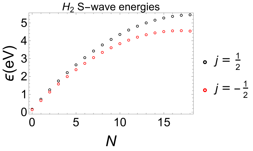
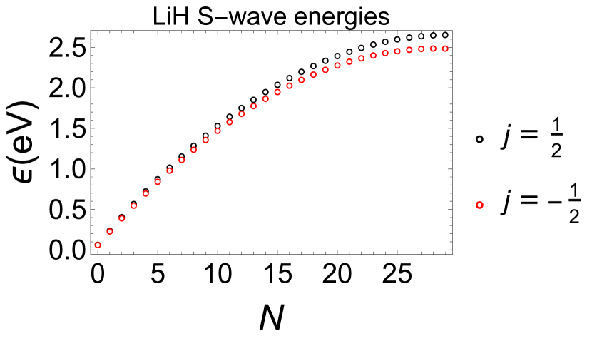
Figure 2: Energies (4) in eV of the $\textrm{H}_{2}$ and the LiH molecules of the allowed S-wave states ($l=0$). In both cases the projection spin $j=+1/2$ increases the energy and the states hold non-degenerated within the ranges $0\leq N\leq 18$ ($\textrm{H}_{2}$) and $0\leq N\leq 29$ (LiH).

4 Thermodynamics of the S-wave states and Morse spectrum finiteness: Schottky effect

We explore the effects of the approximated radial equation (23) in the statistical properties of the S-wave states ($l=0$) that manifest the vibrational features of the system. With the aim to obtain the partition function of the canonical ensemble, we consider that the system is in equilibrium with a thermal bath of finite temperature $T$. We shall consider only the states with positive energy to avoid the negative energies that are unlimited by below, which also guarantees a stable ensemble [50]. For reasons of calculus we recast the formula of the energy

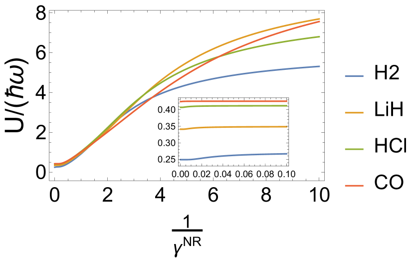
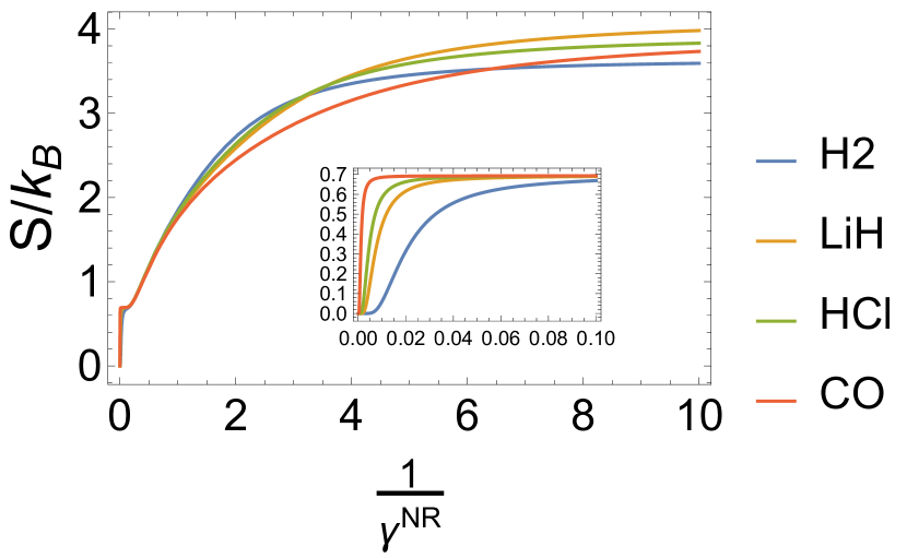
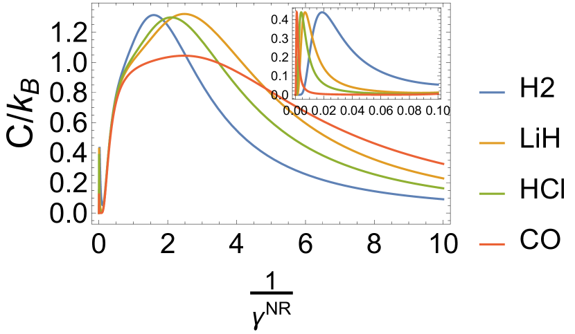
Figure 3: (a) Internal energy (top), (b) entropy (center) and (d) heat capacity (bottom) of the S-wave states ($l=0$) of the $\textrm{H}_{2}$, LiH, HCl and CO molecules in the non-relativistic regime in the presence of the effective radial Morse potential (23) for the Dirac case. The parameters of the Table 2 along with the approximated energy (4) (for $\delta^{2}$ vanishingly small) were employed. Two peaks are observed for the heat capacity (the first one in the inset), in virtue of the finiteness of the energy levels (Schottky effect).

(24) as

$$\mathcal{\widetilde{E}}_{N,j=\pm 1/2}/\hbar\omega=\sqrt{1+\delta(3\pm 2(1+\alpha)/\alpha)}\left(N+\frac{1}{2}\right)\times$$

$$\bigg{[}1-\frac{\alpha^{2}\delta}{2\sqrt{1+\delta(3\pm 2(1+\alpha)/\alpha)}}\left(N+\frac{1}{2}\right)\bigg{]}-\frac{1}{2\alpha^{2}}$$ (28)

where $\pm$ stands for the spin projections $+1/2$ and $-1/2$ respectively. Thus, we can perform two partitions functions

$$Z^{\textrm{NR}}=\sum_{j=\pm 1/2}\sum_{N=0}^{N_{\textrm{max}}}e^{\gamma^{\textrm{NR}}\mathcal{\widetilde{E}}_{N,j=\pm 1/2}/\hbar\omega}$$ (29)

and

$$Z^{\textrm{R}}=\sum_{j=\pm 1/2}\sum_{N=0}^{N_{\textrm{max}}}e^{\gamma^{\textrm{R}}\sqrt{1+2\gamma\mathcal{\widetilde{E}}_{N,j=\pm 1/2}/\hbar\omega}}$$ (30)

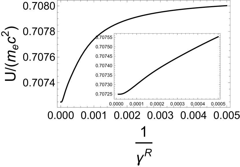
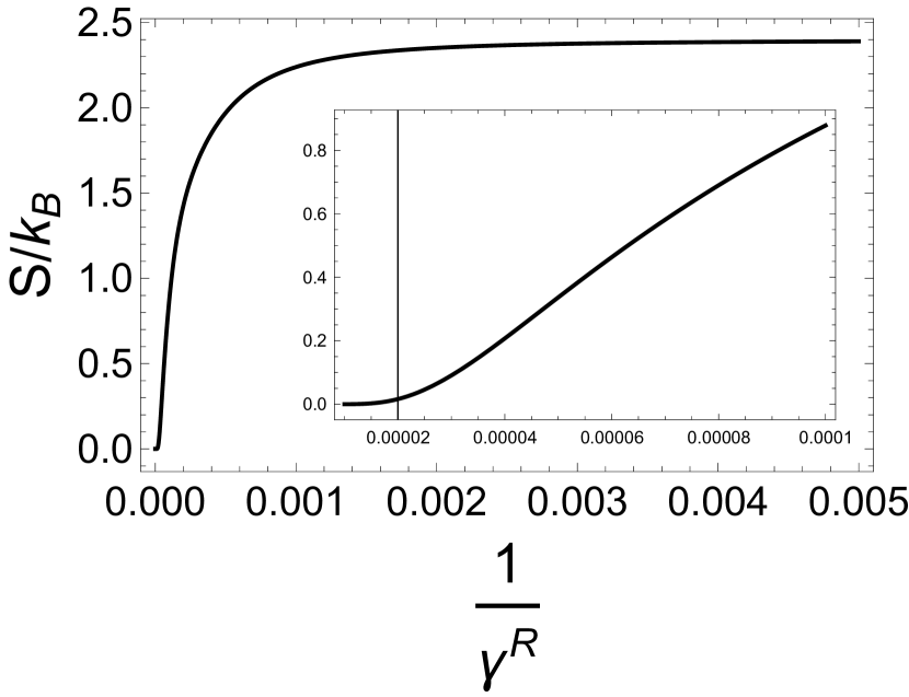
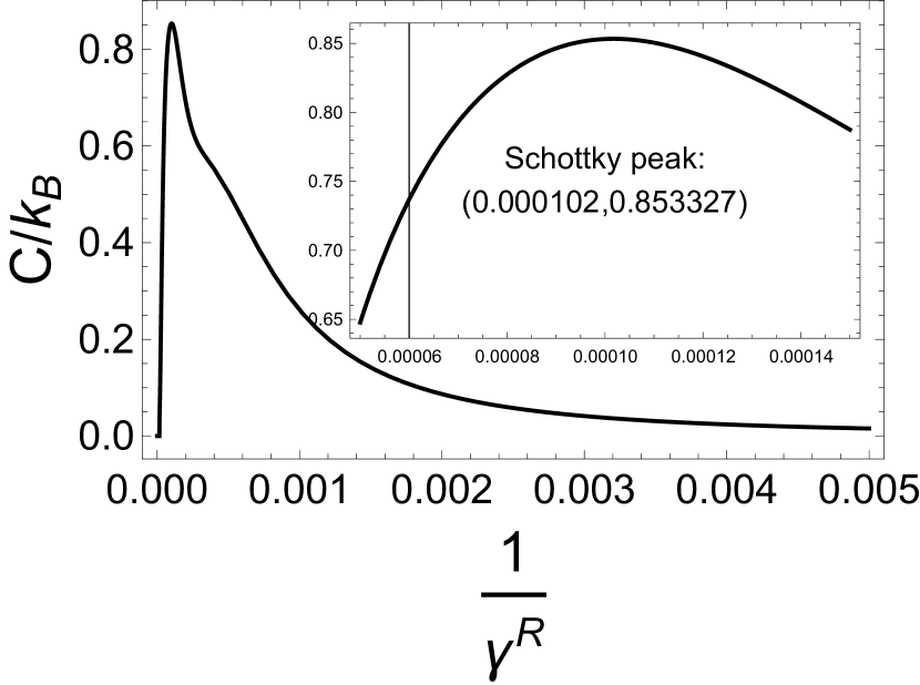
Figure 4: (a) Internal energy (top), (b) entropy (center) and (d) heat capacity (bottom) of the S-wave states ($l=0$) of electrons with $\hbar\omega\sim 124\textrm{eV}$ (ultraviolet spectrum) in the relativistic regime in the presence of the effective radial Morse potential (23) for the Dirac case. The parameters $\gamma=0.000242661=\hbar\omega/m_{e}c^{2}$, $\delta=E_{\textrm{h}}/\hbar\omega=0.219444$ and $\alpha=1$ along with the approximated energy (4) were employed. As in the molecules case, a peak is observed for the heat capacity due to the Schottky effect.

corresponding to the non-relativistic and the relativistic cases. Here the dimensionless parameters $\gamma^{\textrm{NR}}=\frac{\hbar\omega}{k_{B}T}$, $\gamma^{\textrm{R}}=\frac{mc^{2}}{k_{B}T}$ measure the ratios between the vibrational energy and the rest mass energy with respect to the thermal excitations, and $\gamma=\frac{\hbar\omega}{mc^{2}}$ measures the ratio between the vibrational energy and the rest mass one. These coefficients allow to characterize all the regimes of interest from the low to the high temperatures as well as the intermediate ones. It is also assumed that $\gamma$ is fixed for each molecule of the Table 2 in terms of its characteristic parameters. To complete our analysis the (dimensionless) thermodynamical potentials are needed

$$U = -\frac{\partial\ln Z^{\textrm{NR,R}}}{\partial\gamma^{\textrm{NR,R}}}\quad\textrm{(internal energy)}$$

$$F = -\frac{1}{\gamma^{\textrm{NR,R}}}\ln Z^{\textrm{NR,R}}\quad\textrm{(Helmholtz free energy)}$$

$$S = (\gamma^{\textrm{NR,R}})^{2}\frac{\partial F}{\partial\gamma^{\textrm{NR,R}}}\quad\textrm{(entropy)}$$

$$C = -(\gamma^{\textrm{NR,R}})^{2}\frac{\partial U}{\partial\gamma^{\textrm{NR,R}}}\quad\textrm{(heat capacity)}$$ (31)

from which all the thermodynamics of the S-wave states can be derived. For recovering the units of the thermodynamical potentials it is enough to add the energy factor $\hbar\omega$ or $mc^{2}$ in $U$ and $F$, and to add $k_{B}$ in $S$ and $C$. The notations $Z^{\textrm{NR,R}}$ and $\gamma^{\textrm{NR,R}}$ stand for their respective magnitudes in the non-relativistic and relativistic contexts. For the molecules above mentioned the coefficient $\gamma=\hbar\omega/mc^{2}$ results vanishingly small, due to their enormous value of the rest mass $mc^{2}$ (of the order of the $\sim 1000$ Mev) against the small photon energy $\hbar\omega$ characteristic of the level spacements in typical quantum transitions. So, in order to see relativistic effects and to maintain $\delta\ll 1$ we shall consider $\hbar\omega\sim 124\textrm{eV}$, that corresponds to the extreme ultraviolet spectrum, along with $mc^{2}=m_{e}c^{2}=511\textrm{keV}$ (i.e. the rest mass of the electron). In virtue that $\delta=\textrm{E}_{\textrm{h}}/\hbar\omega$ with $\textrm{E}_{\textrm{h}}$ the Hartree energy, we have $\gamma=0.000242661$ and $\delta=0.219444$ so $\delta^{2}=0.0481555$ can be neglected in relation with $\delta$, and then the approximation (4) holds valid. We set $\alpha=-\gamma r_{e}=1$. Thus, the number $N_{\textrm{max}}$ of allowed states for the states with projection spin $1/2$ and $-1/2$ result $6$ and $3$ respectively .

From Figs. 3 and 4 we see the Schottky effect is present in both regimes, the non-relativistic and the relativistic one, due to the finite number of allowed states. The peaks in the heat capacity are physically interpreted due the fact that the more higher is the temperature the less number of states that the system has to be possibly occupied. So when the temperature sufficiently increases that the factor $k_{B}T$ approaches to the difference of the energy levels, a peak in the heat capacity emerges, and from there small changes in the temperature produce changes in the entropy in such a way the heat capacity continues decreasing up to be zero for $T\rightarrow\infty$. For comparing the Dirac and KG cases, the behavior of the Schottky peaks and their critical temperatures for the systems studied is shown in Table 3.

System	$C(T_{c})$ (Dirac)	$C(T_{c})$ (KG)	$T_{c}$ (Dirac)	$T_{c}$ (KG)
$\textrm{H}_{2}$	$0.44$	$1.8\times 10^{-11}$	$-154.1$	$-265.2$
	$1.31$	$1.29$	$9804.4$	$10606.6$
LiH	$0.44$	$7.474\times 10^{-11}$	$-259.2$	$-271.7$
	$1.32$	$1.31$	$4749.6$	$4876.6$
HCl	$0.44$	$1.34\times 10^{-11}$	$-255.1$	$-270.$
	$1.3$	$1.29$	$8750.6$	$8883$
CO	$0.44$	$8.99\times 10^{-11}$	$-269.8$	$-270.5$
	$1.04$	$1.04$	$7435.2$	$7454.71$
$e^{-}$	$0.85$	$1.11$	$6.03\times 10^{5}$	$2.11\times 10^{6}$

Table 3: Schottky peaks (in units of $k_{B}$) of the systems studied and their associated critical temperatures in Celsius for the Dirac and KG cases. The differences between the Dirac and KG cases are appreciable in the low temperature limit (first row of each molecule) or in the relativistic regime (electron case).

We can see that for the molecules the first peaks give place at low temperatures within the range of the $-270\leq T\leq-150$ degrees Celsius, while the second peaks arise in the interval $4700\leq T\leq 10700$ that correspond to thermal energies $k_{B}T$ of the order of the dissociation energy of the molecules $\sim$ eV. For temperatures $T\geq 10700$ the predictions of the Morse model are no longer valid and then the heat capacity exhibits a typical decreasing with the temperature. In the non-relativistic regime of the molecules studied the spin effects are predominant at the low temperature regime $[-270,-150]$, with an appreciable difference in the magnitude order of the values of the peaks of the Dirac and KG cases. On the other hand, for the electron provided with a high energy $\hbar\omega\sim 124$ eV the spin contributions to the heat capacity are visible still at high temperatures $\sim 10^{5}-10^{6}$.

5 General Pekeris approximation revisited: mapping from three-dimensional radial equation to one-dimensional Schrödinger-like equation

In order to solve the generic radial equation (21) with an arbitrary spherical potential $U(r)$, we revisit the generalized Pekeris approximation of [38] by establishing the variable of the Pekeris expansion $y$ in function of the potential coupling $U(r)$, and by deducing the family of potentials from which a mapping onto a Schrödinger equation with non-minimal coupling emerges. More generally, if $U(r)$ represents an spherical radial potential, we can define the dimensionless variable

$$y=\gamma U(r)+1=f^{-1}(\gamma(r-r_{e}))$$ (32)

with $\gamma$ a real parameter having units of distance^-1, $f^{-1}(x)=\gamma U(x/\gamma+r_{e})+1$ and $f(x)=\gamma U^{-1}((x-1)/\gamma)-\gamma r_{e}$. In particular, for the Morse potential coupling $U(r)=(1/\gamma)(e^{\gamma(r-r_{e})}-1)$ we recover the previously used $y=e^{\gamma(r-r_{e})}$ with $f^{-1}(x)=e^{x}$. In order to provide the method, we assume that $U$ has a differentiable inverse $U^{-1}$ and then $f$ and $f^{-1}$ result also differentiable. Thus, from (32) it follows approximated expressions for $r_{e}/r$ and $(r_{e}/r)^{2}$ up to terms of order $2$ around $y=1$ ($r=r_{e}$)

$$r_{e}/r = \left(1+f(y)/(\gamma r_{e})\right)^{-1}\approx\frac{1}{\frac{f(1)}{\gamma r_{e}}+1}+\sum_{i=1}^{2}a_{i}(y-1)^{i}$$

$$(r_{e}/r)^{2} = \left(1+f(y)/(\gamma r_{e})\right)^{-2}\approx\frac{1}{\left(\frac{f(1)}{\gamma r_{e}}+1\right)^{2}}+\sum_{j=1}^{2}a_{j}(y-1)^{j}$$

$$a_{1} = -\frac{\gamma r_{e}f^{\prime}(1)}{\left(\gamma r_{e}+f(1)\right)^{2}}$$

$$a_{2} = -\frac{\left(\gamma r_{e}\left(\gamma r_{e}f^{\prime\prime}(1)+f(1)f^{\prime\prime}(1)-2f^{\prime}(1)^{2}\right)\right)}{2\left(\gamma r_{e}+f(1)\right)^{3}}$$

$$b_{1} = -\frac{2(y-1)\left(\gamma^{2}r_{e}^{2}f^{\prime}(1)\right)}{\left(\gamma r_{e}+f(1)\right)^{3}}$$

$$b_{2} = -\frac{\gamma^{2}r_{e}^{2}\left(\gamma r_{e}f^{\prime\prime}(1)+f(1)f^{\prime\prime}(1)-3f^{\prime}(1)^{2}\right)}{\left(\gamma r_{e}+f(1)\right)^{4}},$$ (33)

which for the Morse potential case result more simplified since $f(1)=0$. For avoiding terms of the type $\propto U^{3}$ in the term $U/r$ in (46) we can still make $a_{2}=0$. Then, using (5) the effective potential (46) can be recasted in terms of $y-1=\gamma U$ for $r\sim r_{e}$ as

$$U_{\mathrm{eff}}(r)\approx\left(\frac{m\omega^{2}}{2\gamma^{2}}-[1+f(j,l)]\frac{\hbar\omega}{\gamma r_{e}}a_{1}+\frac{\hbar^{2}l(l+1)}{2r_{e}^{2}}b_{2}\right)(y-1)^{2}$$

$$+\left(-[1+f(j,l)]\frac{\hbar\omega}{\gamma r_{e}}+\frac{\hbar^{2}l(l+1)}{2r_{e}^{2}}b_{1}\right)(y-1)+\frac{\hbar^{2}l(l+1)}{2r_{e}^{2}}-\frac{\hbar\omega}{2\gamma}\frac{d(y-1)}{dr}$$

$$=A_{1}\gamma^{2}\bigg{[}U(r)+A_{2}/(2\gamma A_{1})\bigg{]}^{2}+A_{3}-A_{2}^{2}/4A_{1}-\frac{\hbar\omega}{2}\frac{U(r)}{dr}$$ (34)

with the pertinent identifications for the constants $A_{1},A_{2},A_{3}$. Hence, we arrive to one of the main results of the paper. For $r\sim r_{e}$ we can map the differential radial equation (21) for an arbitrary spherical potential $U(r)$ such that $U$ and its inverse $U^{-1}$ are differentiable in a neighbouring of $r=r_{e}$ and of $U(r_{e})$ respectively, into the one-dimensional Schrödinger-like equation

$$\mathcal{E}\Phi = \Bigg{\{}-\frac{\hbar^{2}}{2m}\frac{d^{2}}{dr^{2}}+A_{1}\gamma^{2}\bigg{[}U(r)+A_{2}/(2\gamma A_{1})\bigg{]}^{2}$$ (35)

$$+A_{3}-A_{2}^{2}/4A_{1}-\frac{\hbar\omega}{2}\frac{U(r)}{dr}\Bigg{\}}\Phi,$$

that does not contain cross terms of the type $U(r)/r$ nor Coulomb or centrifugal terms as the radial equation (21). The constants $A_{1},A_{2},A_{3}$ are determined by

$$A_{1} = \left(\frac{m\omega^{2}}{2\gamma^{2}}-[1+f(j,l)]\frac{\hbar\omega}{\gamma r_{e}}a_{1}+\frac{\hbar^{2}l(l+1)}{2r_{e}^{2}}b_{2}\right)$$

$$A_{2} = \left(-[1+f(j,l)]\frac{\hbar\omega}{\gamma r_{e}}+\frac{\hbar^{2}l(l+1)}{2r_{e}^{2}}b_{1}\right)$$

$$A_{3} = \frac{\hbar^{2}l(l+1)}{2r_{e}^{2}},$$ (36)

which together with (5) and $f(x)=\gamma U^{-1}((x-1)/\gamma)-\gamma r_{e}$ give a complete proof of the desired mapping. To emphasize its construction, we refer to the formula (35) as a Pekeris mapping. Besides the Morse potential previously studied, next we shall examine other illustrative examples.

5.1 Example 1: modified 12-6-9 Lennard-Jonnes potential

A classical example for modelling the intermolecular interactions between a pair of neutral atoms of molecules is the Lennard-Jones potential, that we can consider in a modified 12-6-9 form

$$V(r)=\epsilon\bigg{[}\left(\frac{r_{e}}{r}\right)^{6}-\sqrt{2}\left(\frac{r_{e}}{r}\right)^{3}\bigg{]}^{2}=V_{LJ}-2\epsilon\sqrt{2}\left(\frac{r_{e}}{r}\right)^{9}$$ (37)

with $\epsilon$ the depth of the potential well and $V_{LJ}$ standing for the Lennard-Jonnes potential. In this case, from the identifications $\epsilon=m\omega^{2}/2\gamma^{2}$ and $\gamma=1/r_{e}$ we deduce the non-minimal coupling $U(r)=(1/\gamma)[(\gamma r)^{-6}-\sqrt{2}(\gamma r)^{-3}]$, and then by inverting $U(r)$ (where we choose the positive branch) it follows $f(x)$

$$f(x)=\left(\frac{2}{\sqrt{2}+\sqrt{2+4(x-1)}}\right)^{1/3}-1,$$ (38)

where $x=1$ corresponds to $U^{-1}(0)$, i.e. the minimum of the potential $r=r_{e}/2^{1/6}$. Having obtained $f(x)$ the Pekeris mapping follows straightforwardly by (5), (35) and (5).

5.2 Example 2: homographic-squared potential

Other type of invertible non-minimal coupling $U(r)$ that we can consider is an homographic-squared potential, expressed by

$$V(r)=\epsilon\left(\frac{a(r/r_{e})+b}{c(r/r_{e})+d}\right)^{2}$$ (39)

which for $c=0,d=1$ and $a=0$; $b,c\neq 0$ collapse in the harmonic and the $1/r^{2}$ potentials respectively. Again, $\epsilon$ represents the strength force of the potential and we can make the identifications $\epsilon=m\omega^{2}/2\gamma^{2}$ and $\gamma=1/r_{e}$. Then, the non-minimal coupling results $U(r)=\frac{1}{\gamma}(a(\gamma r)+b)/(c(\gamma r)+d)$. By inverting the homographic coupling $U(r)$ we obtain

$$f(x)=\frac{-b(x-1)+d}{-c(x-1)+a}-1.$$ (40)

In this case, the choice $f(1)=0$ simplifies the constants $a_{1},b_{1},b_{2}$ of (5) and also implies $a=d$.

5.3 Example 3: Pekeris mapping into Schrödinger equation with non-minimal coupling

We also can consider the special family of non-minimal couplings $U(r)$ satisfying the differential equation

$$\frac{dU}{dr}=\alpha_{2}U^{2}+\alpha_{1}U+\alpha_{0}$$ (41)

with $\alpha_{i}$ ($i=0,1,2$) real coefficients. We notice that (41) and the expressions (35) allow to rewrite the radial equation (21) with the effective potential being a quadratic function of $U$, i.e.

$$\mathcal{E}\Phi = \left[-\frac{\hbar^{2}}{2m}\frac{d^{2}}{dr^{2}}+K_{1}(U(r)-K_{2})^{2}+K_{3}\right]\Phi,$$ (42)

where $K_{1},K_{2},K_{3}$ are constants to be determined (with the help of (5)) and that depend on the quantum numbers $n,j,l$ along with the parameters $m,\gamma,r_{e},\omega,\alpha_{1},\alpha_{2},\alpha_{3}$. In this case we say that the Pekeris mapping is allows to rewrite (42) as

$$2m\mathcal{E}\Phi = [\left(p_{r}-iK_{1}(U(r)-K_{2})\right)\left(p_{r}-iK_{1}(U(r)-K_{2})\right)^{\dagger}$$ (43)

$$+K_{3}]\Phi.$$

that is the free one-dimensional Schrödinger equation dotted with the non-minimal coupling $p_{r}-iK_{1}(U(r)-K_{2})$ in the $r$-direction. By solving (41) we find out what are the potentials that belong to the Pekeris mapping (42), which are given by

$$U(r)=\sqrt{4\alpha_{0}\alpha_{2}-\alpha_{1}^{2}}\times$$ (44)

$$\frac{\tan\left[\frac{1}{2}\left(\sqrt{4\alpha_{0}\alpha_{2}-\alpha_{1}^{2}}K+\sqrt{4\alpha_{0}\alpha_{2}-\alpha_{1}^{2}}r\right)\right]-\alpha_{1}}{2\alpha_{2}}$$

with $K$ an arbitrary integration constant. Some representative non-minimal couplings generated by the family (44) are shown in Table 4.

coupling type	$\alpha_{2}$	$\alpha_{1}$	$\alpha_{0}$	$U(r)$
tangent	$1$	$0$	$1$	$\tan\left(r+K\right)$
Morse	$<0$	$0$	$\alpha_{2}$	$Ke^{\alpha_{2}r}-1$
Coulomb	$\neq 0$	$0$	$0$	$(-\alpha_{2}r-K)^{-1}$
harmonic	$0$	$0$	$>0$	$\alpha_{0}r+K$
quotient exponential	$\neq 0$	$\alpha_{2}$	$0$	$-e^{K+\alpha_{2}r}/(e^{K+\alpha_{2}r}-1)$

Table 4: Some characteristic couplings belonging to the family (44). Their Pekeris mappings correspond to a Schrödinger equation with a non-minimal coupling $U(r)$, given by (43).

6 Conclusions

We have presented the one-dimensional and the three-dimensional relativistic equations for the Morse potential that result from a generalized momentum operator provided with a deformed non-minimal coupling. By means of the Pekeris approximation in the 3D case we have converted the not exactly solvable radial wave equation (21) into the Morse-like equation (23), whose solutions and energies are obtained by a mapping onto the one-dimensional Morse problem (5), corresponding to the vibrational states ($r\sim r_{\mathrm{e}}$). We have recovered the non-relativistic energies of the S-wave states of the $\textrm{H}_{2}$ in a very good agreement (Table 1) and we have shown that the Pekeris approximation gives a good accuracy of the Coulomb and centrifugal terms (Fig. 1) within the range $r_{e}/2\leq r\leq 3r_{e}/2$.

For the three-dimensional case and employing the Pekeris approximation (7), we have seen that the corrections of the spin and momentum angular contributions to the one-dimensional Morse energies (7) are contained in the effective angular frequency $\Omega^{2}=\omega^{2}\left[+\delta\left(3+2(1+f(j,l))\frac{1+\alpha}{\alpha}+l(l+1)\frac{\alpha^{2}+3\alpha+2}{\alpha}\right)\right]$, leading to the energy formula (4), which is valid for the $\textrm{H}_{2}$, LiH, HCL and CO molecules when $\delta\ll 1$ (Table 2). We have illustrated the spin effect to the Dirac energies of the S-wave states with the $\textrm{H}_{2}$ and LiH molecules, where an splitting in the energies is evidenced (Fig. 2). Regarding the thermodynamical properties, for the molecules studied and for a high energy electron in the non-relativistic and relativistic regimes respectively, we have reported Schottky effects in the heat capacity due to the finiteness of the allowed spectrum of the Morse potential (Figs. 3 and 4). In the Dirac and KG systems, the Schottky peaks express the screening of the spin contributions to the heat capacity (caused by thermal excitations), thus making them appreciable at low temperatures in the non-relativistic regime or at high temperatures in relativistic particles (Table 3).

By revisiting the generalized Pekeris approximation [38], we have established the functional form $f(x)=\gamma U^{-1}((x-1)/\gamma)-\gamma r_{e}$ of the expansion variable $y=f^{-1}(\gamma(r-r_{e}))$, and we have extended this perspective to the relativistic domain. Thus, given $U(r)$ we have a Pekeris mapping from the three-dimensional KG and Dirac equations to a one-dimensional like Schrödinger equation, given by Eqns. (5) (35) and (5). We have illustrated the complexity of the Pekeris mapping for the 12-6-9 Lennard-Jones and the homographic-squared potentials. Moreover, we have obtained the family of non-minimal couplings whose Pekeris mapping becomes into a one-dimensional Schrödinger equation provided with a minimal coupling (44), from which the tangent, Morse, Coulomb, harmonic and the quotient exponential result to be special cases (Table 4).

7 Appendix

We have that up terms of second order [37, 38]

$$r_{\mathrm{e}}/r=\left(1+\ln y/\gamma r_{\mathrm{e}}\right)^{-1}\approx 1-\frac{1}{\gamma r_{\mathrm{e}}}(y-1)$$

$$+\frac{2+\gamma r_{\mathrm{e}}}{2(\gamma r_{\mathrm{e}})^{2}}(y-1)^{2}$$

$$(r_{\mathrm{e}}/r)^{2}=\left(1+\ln y/\gamma r_{\mathrm{e}}\right)^{-2}\approx 1-\frac{2}{\gamma r_{\mathrm{e}}}(y-1)$$

$$+\frac{3+\gamma r_{\mathrm{e}}}{(\gamma r_{\mathrm{e}})^{2}}(y-1)^{2}$$ (45)

with $y=e^{\gamma(r-r_{\mathrm{e}})}$ and the expansions are around $y=1$ ($r=r_{\mathrm{e}}$). The effective potential of the radial equation (21) is

$$U_{\mathrm{eff}}(r)=\frac{m\omega^{2}}{2}U^{2}-\frac{\hbar\omega}{2}\frac{dU}{dr}-[1+f(j,l)]\frac{\hbar\omega U}{r}+\frac{\hbar^{2}l(l+1)}{2mr^{2}}.$$ (46)

In order to adimensionalize variables we set $-\gamma r_{e}=\alpha>0$ and $\hbar/(m\omega r_{e}^{2})=\delta>0$. Thus, replacing $U=\frac{e^{\gamma(r-r_{e})}-1}{\gamma}$ and the Pekeris approximated expressions of $r_{\mathrm{e}}/r,(r_{\mathrm{e}}/r)^{2}$ of (7) in (46) we can rewrite the effective potential $U_{\textrm{eff}}(r)$ as

$$U_{\textrm{eff}}(r)=\frac{m\Omega^{2}}{2\gamma^{2}}\left[e^{\gamma(r-r_{\textrm{eff}})}-1\right]^{2}+U_{0}$$

where

$$\Omega^{2}=\omega^{2}A\left(1-\frac{B}{2A}\right)^{2}$$

$$r_{\mathrm{eff}}=r_{\mathrm{e}}+\frac{1}{\gamma}\ln\left(1-\frac{B}{2A}\right)$$

$$U_{0}=\frac{m\Omega^{2}}{2\gamma^{2}}\left(C-\frac{B^{2}}{4A}\right)$$

and

$$A=1+\delta\left(2(1+f(j,l))+l(l+1)(3-\alpha)\right)$$

$$B=-\delta\left[1-2\frac{1+f(j,l)}{\alpha}-2\frac{l(l+1)}{\alpha}\right]$$

$$C=\delta\left[(l+1)-1\right]$$

References

• [1] P. A. M. Dirac, The Principles of Quantum Mechanics, Oxford University Press, Oxford, 1930.
• [2] M. Moshinsky and A. Szczepaniak, J. Phys. A: Math. Gen. 22, L817 (1989).
• [3] S. Bruce and P. Minning, Il Nuovo Cimento A 106, 711-713 (1993); Il Nuovo Cimento A 107, 169 (1994).
• [4] V. V. Dvoeglazov, Il Nuovo Cimento A 107, 1413 (1994).
• [5] J. S. Kang J. S. and H. J. Schnitzer, Phys. Rev. D 12, 841 (1975).
• [6] H. Akcay, J. Phys. A: Math. Theor. 40, 6427-6432 (2007).
• [7] K. Bakke and C. Furtado, Ann. Phys. 355, 48-54 (2015).
• [8] R. Rivelino, E. S. Santos and M. Montigny, Int. J. Theor. Phys. 54, 85-91 (2015).
• [9] H. Benzair, T. Boujdjedaa and M. Merad, Eur. Phys. J. Plus 132, 94 (2017).
• [10] M. D. Oliveira and A. G. M. Schmidt, Ann. Phys. 401, 21-39 (2019).
• [11] A. Merad, M. Aouachria, M. Merad and T. Birkandan, Int. J. Mod. Phys. A 34, 1950218 (2019).
• [12] V. Tyagi, S. K. Rai and B. P. Mandal, EPL 128, 30004 (2020).
• [13] R. N. Costa Filho, M. P. Almeida, G. A. Farias and J. S. Jr. Andrade, Phys. Rev. A 84, 050102(R) (2011).
• [14] R. N. Costa Filho, G. Alencar, B.-S. Skagerstam and J. S. Jr. Andrade, EPL 101, 10009 (2013).
• [15] R. N. Costa Filho, J. P. M. Braga, J. H. S. Lira and J. S. Andrade, Phys. Lett. B 755, 367 (2016).
• [16] P. M. Morse, Phys. Rev. 34, 57 (1929).
• [17] B. G. da Costa, I. S. Gomez and A. M. F. dos Santos, EPL 129, 10003 (2020).
• [18] A. D. Alhaidari, Phys. Rev. Lett. 87, 210405 (2001); Phys. Rev. Lett. 87, 249901 (2001); Phys. Rev. Lett. 88, 189901 (2002).
• [19] A. N. Vaidya and R. L. Rodrigues, Phys. Rev. Lett. 89, 068901 (2002);
• [20] A. D. Alhaidari, Phys. Lett. A 326, 58-69 (2004).
• [21] G. Chen, Phys. Lett. A 339, 300-303 (2005).
• [22] A. D. Alhaidari, H. Bahlouli and A. Al-Hassan, Phys. Lett. A 349, 87-97 (2006).
• [23] C. Berkdemir, Nucl. Phys. A 770, 32 (2006); Nucl. Phys. A 821, 262 (2009).
• [24] W-C. Qiang, R-S. Zhou and Y. Gao, J. Phys. A: Math. Theor. 40, 1677-1685 (2007).
• [25] L-H. Zhang, X-P. Li and C-H. Jia, Phys. Scr. 80, 035003 (2009).
• [26] O. Bayrak, A. Soylu and I. Boztosun, J. Math. Phys. 51, 112301 (2010).
• [27] T. T. Ibrahim, K. J. Oyewumi and S. M. Wyngaart, Eur. Phys. J. Plus 127, 100 (2012)
• [28] S. Ortakaya, Ann. Phys. 338, 250-259 (2013).
• [29] X.-J. Xie and C.-S. Jia, Phys. Scr. 90, 035207 (2015).
• [30] P. Zhang, H-C. Long and C-H. Jia, Eur. Phys. J Plus 131, 117 (2016).
• [31] M. G. Garcia, A. S. Castro, L. B. Castro and P. Alberto, Ann. Phys. 378, 88-99 (2017).
• [32] M. G. Garcia, A. S. Castro, P. Alberto and L. B. Castro, Phys. Lett. A 381, 2050-2054 (2017).
• [33] E. J. A. Curi, L. B. Castro and A. S. Castro, Eur. Phys. J Plus 134, 248 (2019).
• [34] I. Nasser, M. S. Abdelmonem, H. Bahlouli and A. D. Alhaidari, J. Phys. B: At. Mol. Opt. Phys. 40, 4245 (2007).
• [35] E. Castro, J. L. Paz and P. Martin, J. Mol. Struct.: Theochem. 769, 15 (2006).
• [36] J. ZΓΊΓ±iga, A. Batisda and A. Requena, Jour. Chem. Educ. 85, 1675 (2008).
• [37] C. L. Pekeris, Phys. Rev. 45, 98 (1993).
• [38] F. J. S. Ferreira and F. V. Prudente, Phys. Lett. A 377, 3027-3032 (2013).
• [39] S. H. Mazharimousavi, Phys. Rev. A 85, 034102 (2012).
• [40] B. G. da Costa and E. P. Borges, J. Math. Phys. 55, 062105 (2014).
• [41] B. G. da Costa and I. S. Gomez, Phys. Lett. A 382, 2605 (2018).
• [42] C. Tsallis, J. Stat. Phys. 52, 459 (1988).
• [43] C. Tsallis, Braz. J. Phys. 29, 1-35 (1999).
• [44] F. D. Nobre, M. A. Rego-Monteiro and C. Tsallis, Phys. Rev. Lett. 106, 140601 (2011).
• [45] E. P. Borges, Phys. A 340, 95 (2004).
• [46] D. J. BenDaniel and C. B. Duke, Phys. Rev. 152, 683 (1966).
• [47] L. Serra and E. Lipparini, EPL 40, 667 (1997).
• [48] G. Arfken and H. J. Weber, Mathematical Methods for Physicists, Elsevier Academic Press, London, 2005.
• [49] A. Boumali, A. Hadfdallah and A. Toumi, Phys. Scr. 84, 037001 (2011).
• [50] M. H. Pacheco, R. V. Maluf, C. A. S. Almeida and R. R. Landim, EPL 108, 10005 (2014).