Generalized Reinforcement Meta Learning for Few-Shot Optimization

Abstract

We present a generic and flexible Reinforcement Learning (RL) based meta-learning framework for the problem of few-shot learning. During training, it learns the best optimization algorithm to produce a learner (ranker/classifier, etc) by exploiting stable patterns in loss surfaces. Our method implicitly estimates the gradients of a scaled loss function while retaining the general properties intact for parameter updates. Besides providing improved performance on few-shot tasks, our framework could be easily extended to do network architecture search. We further propose a novel dual encoder, affinity-score based decoder topology that achieves additional improvements to performance. Experiments on an internal dataset, MQ2007, and AwA2 show our approach outperforms existing alternative approaches by 21%, 8%, and 4% respectively on accuracy and NDCG metrics. On Mini-ImageNet dataset our approach achieves comparable results with Prototypical Networks. Empirical evaluations demonstrate that our approach provides a unified and effective framework.

1 Introduction

The key idea of machine learning is to learn patterns from data, and it is important to use informative representations. One of the areas where deep learning excels is through the ability to learn the representations automatically and hierarchically. Structured representations remove the need of handcrafted features while capturing complex patterns from data. Typically the superior performance of deep learning requires massive amounts of training data and often performs poorly in small data settings. Few-shot learning (Miller et al., 2000; Lake et al., 2011; Koch, 2015; Santoro et al., 2016; Vinyals et al., 2016; Ravi & Larochelle, 2017; Finn et al., 2017a; Snell et al., 2017) aims to produce an effective model (ranker, classifier, etc) given only a few examples from each domain/class. After training, the model can generalize to new domains/classes not seen in training. Although this is a hard task, humans are exceptionally good at it. This learning technique also has practical applications. For example, in the context of Voice Assistants, often there is variance from Speech and NLU (Natural Language Understanding) sub-systems. A DM (Decision Making) sub-system consumes the outputs of Speech and NLU sub-systems to choose the best intent and DM should be able to preserve and leverage the knowledge from previous feature distributions. There are other practical applications like Robotics (Finn et al., 2017b; Gui et al., 2018) and Autonomous Systems (Xu et al., 2018) where learning capability of this sort is critical.

In the few-shot regime, the standard optimizers typically do not generalize well. In traditional model training, typically one only focuses on the network blocks used in the models, viz., LSTMs, CNNs, activation functions, tuning model parameters. But the optimization block mostly stays static: experts design it, iterating on theoretical analysis and empirical validations. Some of the popular hand-engineered optimization algorithms are AdaGrad (Duchi et al., 2011), RMSProp (Tieleman & Hinton, 2012), and Adam (Kingma et al., 2014), to name a few. A step-size adaption scheme (Rolinek & Martius, 2016) improves on these existing hand-engineered optimization algorithms. Attacking the few-shot problem by modifying optimization algorithms is a known approach. Optimization algorithm can be learned using guided policy search (Li & Malik, 2016). Some approaches learn both the weight initialization and the optimizer (Ravi & Larochelle, 2017), while few other approaches use a gradient obtained through a gradient to update parameters (Finn et al., 2017a).

In this paper, we propose to learn the optimization algorithm by observing its execution and implicitly scaling the loss surface while retaining the correct gradient direction intact to reach the best optimum and update model parameters accordingly. We propose to learn an optimization algorithm that updates the model parameters in such a way that when executed on test/blind data, it lands in the optimum on the respective loss-surface. In Section 3, we describe the meta-learning framework to learn the optimization algorithm followed by introducing a novel encoder-decoder architecture in Section 4.

2 Related Work

Our work is an intersection of three critical areas of machine learning: meta-learning, optimization and few-shot learning. Below we present related work in each of the three main fields of our work, and later we present related work that combines the three areas.

Meta-Learning: Meta Learning or Learning to Learn (Baxter et al., 1995; Brazdil et al., 1998; Vilalta & Drissi, 2002; Brazdil et al., 2008; Thrun & Pratt, 2012) has a long history, and it is an important building block in Artificial Intelligence. In this approach, we have a meta-learner and a learner (sub-system that learns from a meta-learner), where experience is gained by exploiting meta-knowledge extracted from a sequence of episodes on a dataset. There are two popular perspectives on how meta-knowledge should be learned, and we present them below.

One form is learning common patterns among a family of tasks presented in the training dataset so that the learner can quickly adapt to unseen tasks from the same family. This form of learning is also termed as Transfer Learning or Multi-task Learning. Another form is to learn the correlation between latent structures of tasks and different learners so that the meta-learner produces the best learner that achieves the best performance on the target task.

Networks that learn to modify their own weights over a number of update steps on an input have been studied well (Bengio et al., 1990; Schmidhuber, 1990; Bengio et al., 1992; Hochreiter et al., 2001; Andrychowicz et al., 2016). The use of RL for meta-learning (Duan et al., 2016; Wang et al., 2016), and how network architecture search can be meta-learned using policy-gradient update (Zoph & Le, 2017) have been explored.

Optimization: The move from manual feature engineering to an automated paradigm (deep learning) has been very successful. In spite of this, optimization algorithms are still designed by hand. The idea of automatic step-size adaption for stochastic gradients is popular and different strategies were proposed; one line of work casts the learning rate as a parameter to train via gradient descent (Baydin et al., 2017), while another approach is to use $2^{nd}$ order information (Byrd et al., 2016; Recht & Rahimi, 2017). There have been meta-learning approaches to learn the optimization algorithm, where a gradient descent approach is used (Andrychowicz et al., 2016), and a guided policy search is used (Li & Malik, 2016). Adding proposed parameters to the update rule (Rolinek & Martius, 2016) improves over existing optimizers (like Adam (Kingma et al., 2014)).

Few-Shot Learning: The best-performing methods for few-shot learning have been mainly metric learning methods. Siamese networks (Koch, 2015) train CNNs to encode data in such a way that data points from the same class are closer while from the different classes are far apart. Matching networks (Vinyals et al., 2016) use recurrence with an attention mechanism. Prototypical Networks (Snell et al., 2017) compute a multi-dimensional representation through a learnable embedding function which serves as a prototype for each class. Prototypical Networks are equivalent to Matching Networks for a one-shot scenario while they differ in the few-shot case.

Optimization for Few-Shot Meta-Learning: The goal of few-shot meta learning is to train a learner (model) on a small dataset pertaining to some tasks, which can quickly adapt to new tasks. A memory-augmented neural network (Santoro et al., 2016) can be trained to learn how to store and retrieve memories for each classification task. Approaches learning both weight initialization and the optimizer (Ravi & Larochelle, 2017), for few-shot image recognition, has been shown to empirically outperform metric learning methods (Koch, 2015; Vinyals et al., 2016). In other approaches parameters are updated using a gradient through a gradient (Finn et al., 2017a).

Unlike these methods, our approach GRE-METL (Generalized REinforcement METa Learning) learns an optimization algorithm based on policy gradients while also learning network architecture. Learning network architecture using RL is also proposed in (Zoph & Le, 2017), we extended that work to learn optimization for the few-shot regime.

3 Task Description and Methodology

3.1 Task Description

Our goal is to generalize to different tasks (ranking, classification) coming from a distribution of tasks P(T) that belongs to the same family. In meta-learning, we work with meta-sets: we have a meta-set $D_{meta}$ which we assume is from P(T), and we have $D_{meta-train}$ and $D_{test}$ from $D_{meta}$. Traditionally in few-shot tasks, we consider k-shot, N-class learning tasks, where for each $D_{train}$ (a sample from $D_{meta-train}$) we have k labeled data points for each of N classes. We want to do well on $D_{test}$. We first split the training data $D_{meta-train}$ into different static mini-batches ($D_{train}$) by random sampling. Dynamic mini-batches modify the intra-distribution of tasks during training in every meta-epoch which will make the training to not converge. Given a model with some parameters $f(X,\theta)$, each task ($D_{train}$) from a training set will have a loss surface with respect to the parameters $\theta$. Similarly unseen tasks will also have their respective loss surfaces. The key idea is to find - instead of optimal parameters for a specific train loss surface - a way to get the optimal parameters that not only perform better on seen loss surfaces but also on unseen loss surfaces pertaining to the same task family P(T), i.e. L($f(X_{test};\theta)$, $Y_{test}$) on the test loss surface should be close to the optimum. Our intuition here is that these loss surfaces would have common structures since they are from same task family, and basing optimization on these commonalities should lead to better generalization. We empirically test our intuition on one internal and three benchmark datasets.

3.2 Methodology

The core idea is to transform the loss surface $L$ to $L^{{}^{\prime}}$ while retaining the general properties of the objective function. To illustrate, we take the simple example of a 2-dimensional convex function in Figure 1 where we obtain gradients of scaled loss surface to update parameters, this has two advantages:

• Captures commonalities among different loss surfaces from the same distribution of tasks to predict the best navigation path to the optimum.

• Faster convergence.

To formulate, let $X,$ $Y,$ and $\theta$ denote feature vectors, labels, and model parameters respectively.

$$L=\textit{L($f(X;\theta)$, $Y$)}$$ (1)

The transformer function $\phi$ scales the loss function $L$ to produce $L^{{}^{\prime}}$. The transformed loss surface $L^{{}^{\prime}}$ possess the same general properties as of $L$, and the gradients of $L^{{}^{\prime}}$ build the path towards the optimum.

$$L^{{}^{\prime}}=\phi(L;\lambda_{1},..,\lambda_{n})$$ (2)

where $\lambda_{i}$ corresponds to a single or group of parameters, the latter is preferred when those parameters are optimizing for the same sub-task, and this is explained further in Section 5.

The gradients of the transformed loss function $L^{{}^{\prime}}$ would then be used to update the model parameters:

$$\theta_{t}=\theta_{t-1}-\alpha\bigtriangledown_{\theta}L^{{}^{\prime}}$$ (3)

This algorithm is shown in Algorithm 1. But it is hard to formulate the transformer $\phi$. We show the empirical approximation for Algorithm 1 in Algorithm 2. We propose an RL-based meta-learning scheme that learns an optimization algorithm based on a policy $\pi$ that implicitly does this transformation and obtains the gradients. The key insight here is since we are linearly transforming the loss function $L$ to get $L^{{}^{\prime}}$, the gradient of $L^{{}^{\prime}}$ is also some linear transformation of the gradient of $L$. Let the gradient-scaling coefficients be $\lambda^{{}^{\prime}}_{i}$ corresponding to $\theta_{i}$, then the approximation of the gradients is given as:

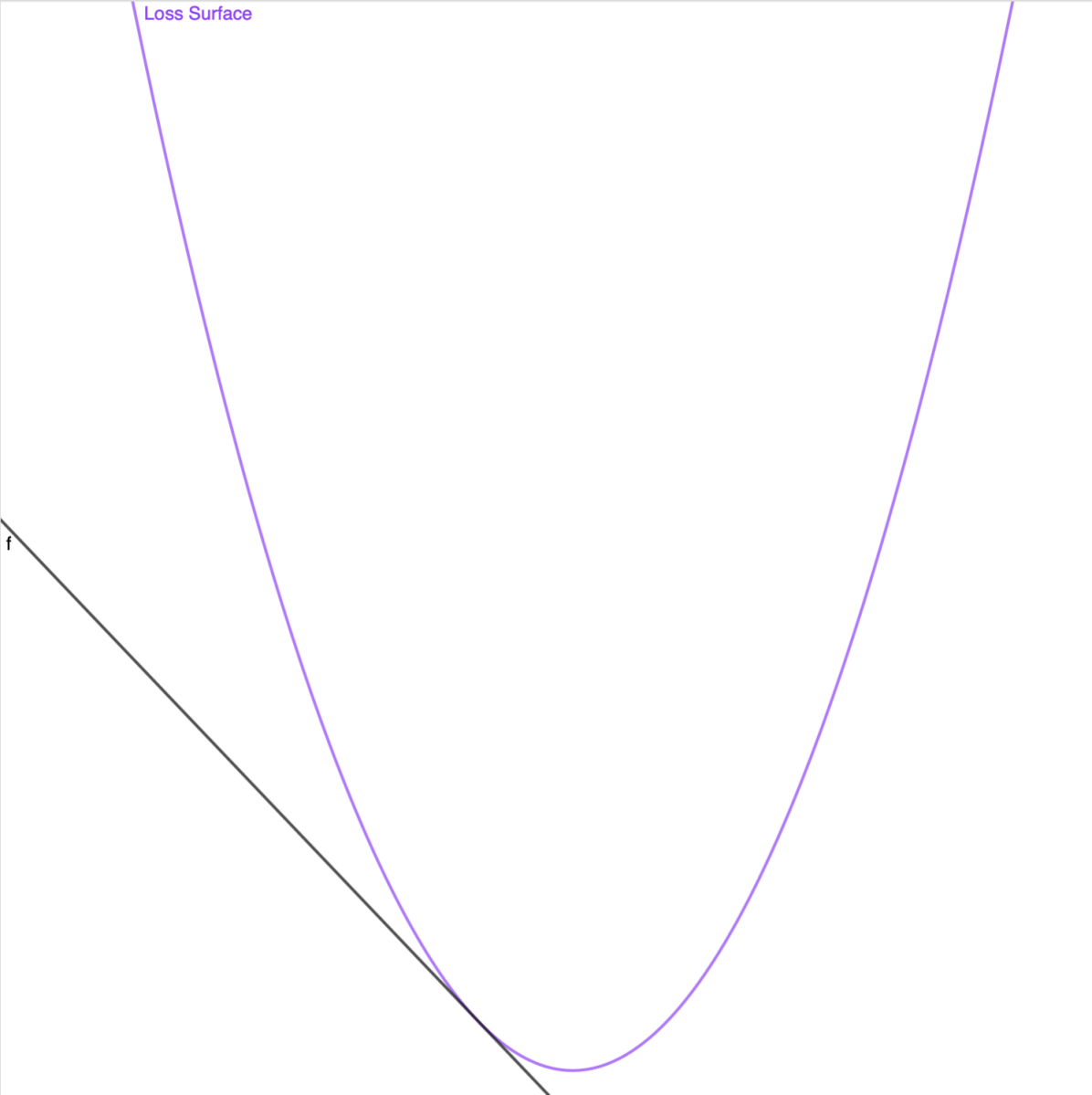
(a) $L$

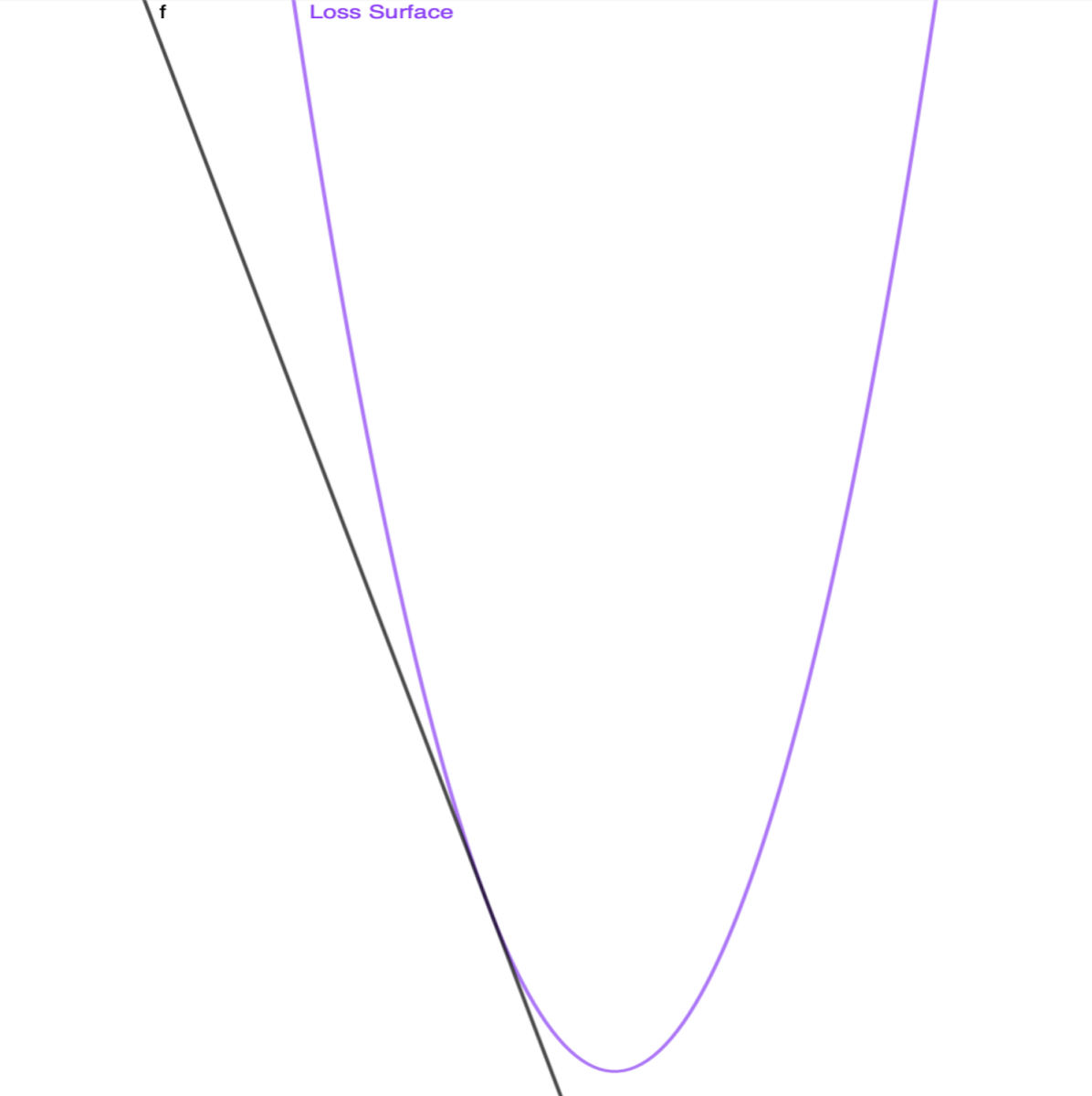
(b) $L^{{}^{\prime}}$ = $\phi(L;\lambda_{1},..,\lambda_{n})$

Figure 1: Actual and transformed loss surfaces with the same general properties.

Require:  P(T) ;

  $\triangleright$ distribution of tasks

Require:  $\phi(.)$ ;

  $\triangleright$ transformer function

$\theta\leftarrow\hskip 4.26773pt$random initialization;

while not done do

       sample$\hskip 5.69046pt\textit{$D_{meta}$}\sim\textit{P(T)};$

      get  $D_{meta-train}$, $D_{heldout}$  from$\hskip 5.69046pt\textit{$D_{meta}$};$

      forall $\textit{$D_{train}$}\hskip 5.69046ptin\hskip 5.69046pt\textit{$D_{meta-train}$}$ do

            

            $Y^{{}^{\prime}}\leftarrow f(X;\theta)$ ;

              $\triangleright$ predicted label

            

            $L\leftarrow L(Y^{{}^{\prime}},Y)$ ;

              $\triangleright$ compute loss

            

            $\bigtriangledown_{\theta}L^{{}^{\prime}}\leftarrow\bigtriangledown_{\theta}(\phi(L))$ ;

              $\triangleright$ compute gradients of transformed loss

            

            $\theta_{t}\leftarrow\theta_{t-1}-\alpha\bigtriangledown_{\theta}L^{{}^{\prime}}$ ;

              $\triangleright$ parameter update

            

            $compute\hskip 5.69046ptand\hskip 5.69046pttrack\hskip 5.69046pt\newline accuracy\hskip 5.69046ptfor\hskip 5.69046pt(X_{heldout},Y_{heldout})\in D_{heldout};$

       end forall

      

end while

Algorithm 1 Directly transforming the loss surface

$$\bigtriangledown^{{}^{\prime}}_{\theta}L^{{}^{\prime}}=\lambda^{{}^{\prime}}_{i}\bigtriangledown_{\theta}L$$ (4)

$$\theta_{t}=\theta_{t-1}-\alpha\bigtriangledown^{{}^{\prime}}_{\theta}L^{{}^{\prime}}$$ (5)

We learn these gradient-scaling coefficients $\lambda^{{}^{\prime}}_{i}$ through a meta-learner that is trained using RL. In every meta-epoch (epoch of meta-learner), it generates $\lambda^{{}^{\prime}}_{i}$, and a sequence of model architecture parameters. This is done based on the action picked by the meta-learner from the space of actions A, $a_{1}$ to $a_{t}$. For every epoch of learner (the sub-system that learns from the meta-learner) in a meta-epoch, we compute the accuracy R on the held-out dataset and use this as the reward signal for the meta-learner. We use a policy-gradient method to iteratively update meta-learner parameters $\theta_{meta}$: the REINFORCE rule from (Williams, 1992), also used in previous works (Zoph & Le, 2017), given below:

$$\bigtriangledown_{\theta_{meta}}P=\bigtriangledown_{\theta_{meta}}\log P(a_{t}|a_{(t-1):1};\theta_{meta})R$$ (6)

$$\bigtriangledown_{\theta_{meta}}L=\sum_{t=1}^{T}E_{P(A,\theta_{meta})}[\bigtriangledown_{\theta_{meta}}P]$$ (7)

To minimize regret, in every meta-epoch we randomly sample from a uniform distribution of [0.0, 1.0] and based on the threshold we either explore or exploit.

Require:  $D_{meta}$  from  P(T);

get  $D_{meta-train}$, $D_{heldout}$, $D_{test}$  from  $D_{meta};$

$\theta_{meta}\leftarrow\hskip 4.26773pt$random initialization;

define $p_{explore}$ ;

  $\triangleright$ probability to decide when to explore vs exploit

while meta-epochs not done do

      

      explore $\leftarrow$ random_draw $\in$ [0.0, 1.0] ;

        $\triangleright$ to minimize regret and trade-off exploration vs exploitation

      

      if $(1^{st}\hskip 4.26773ptepoch)\hskip 4.26773pt\textbf{OR}\hskip 4.26773pt(explore\hskip 4.26773pt<\hskip 4.26773ptp_{explore})$  then

             $\triangleright$ explore

            

            randomly choose $\lambda_{1}$, …, $\lambda_{n}$, and $\theta_{hyper};$

       else

            

            $\triangleright$ exploit

            

            update policy $\pi$ with Equation-7;

            meta-learner $M_{meta}$ picks actions $a_{\lambda}$ $\in$ $A_{\lambda}$ and $a_{hyper}$ $\in$ $A_{hyper}$ that generates $\lambda_{1}$ $\dots$ $\lambda_{n}$, and hyperparameters $\theta_{hyper}$ respectively;

      

      foreach $D_{train}$  in  $D_{meta-train}$ do

            

            $Y^{{}^{\prime}}\leftarrow f(X;\theta)$ ;

              $\triangleright$ predicted label

            

            $L\leftarrow L(Y^{{}^{\prime}},Y)$ ;

              $\triangleright$ compute loss

            

            $\bigtriangledown^{{}^{\prime}}_{\theta}L^{{}^{\prime}}=\phi(\bigtriangledown_{\theta}L;\lambda^{{}^{\prime}}_{1}\dots\lambda^{{}^{\prime}}_{n})$ ;

              $\triangleright$ get scaled gradients

            

            $\theta_{t}=\theta_{t-1}-\alpha\bigtriangledown^{{}^{\prime}}_{\theta}L^{{}^{\prime}}$ ;

              $\triangleright$ update learner’s parameters with scaled gradients

            

            $R\leftarrow getHeldOutAccuracy(.)$

            update policy $\pi$ using Equation-7;

            meta-learner $M_{meta}$ picks action $a_{\lambda}$ $\in$ $A_{\lambda}$ that generates $\lambda_{1}$ $\dots$ $\lambda_{n}$;

            track accuracy on $D_{heldout}$;

       end foreach

      

      $R\leftarrow getTestAccuracy(.)$ ;

        $\triangleright$ get reward on $D_{test}$ from learner with best heldout accuracy

      

end while

Algorithm 2 Empirical approximation of Algorithm 1

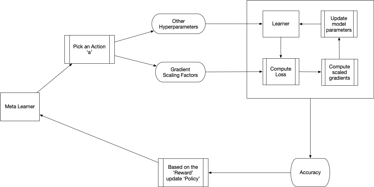
Figure 2: Flow Diagram of Algorithm 2. Meta Learner for every meta-epoch chooses from a set of actions that selects hyperparameters and gradient scaling factors for the Learner. Learner for every epoch updates its parameters using the loss scaled by gradient scaling factors. The best Learner model is chose based on a heldout dataset, and its accuracy is used as the Reward to update the Meta Learner’s policy for choosing actions.

4 Dual Encoder, Affinity-score based Decoder Topology

4.1 Motivation

In many real-world problems different groups of features capture various aspects of the input. For instance, in Voice Assistants, semantic aspects are extracted from ASR (Automatic Speech Recognition) and NLU modules. The outputs of many of these components include score distributions and categorical values. Relevance and Executability aspects are captured by user-data and consists of categorical and numeric features. Conceptually learning the correlation among such feature groups captured in a metric space is an efficient and effective way of decoding correct insights from unseen domains/classes. We investigated the idea of hierarchically encoding these groups of features independently, and then learning the correlation among them as captured by an affinity score vector in metric space. Finally, we decode the affinity score vector to predict the right action/class.

4.2 Dual Encoders

We evaluated this architecture topology by training models on an internal dataset and Animals with Attributes 2 (AwA2) (see Table 1 and Table 4 for results, and Section 5.1 for datasets description). Since both these datasets have two feature groups we used two encoders. It is trivial to expand this idea to multiple ($>2$) encoders. Embeddings are learned for different groups of features from different encoders as shown in Figure 3. Different network architectures can be used for different encoders as best suited by the type of data. We observed that leaving the user-data features from the internal dataset and numeric attributes from AwA2 dataset as static (i.e., non-trainable) results in best performance.

4.3 Affinity Decoder and Shared-trainable Initialization

Once we have the encodings for feature groups, we first learn the correlation among these encodings to learn the affinity vector. We use a bidirectional RNN to learn the affinity-score function. We chose GRU (Cho et al., 2014) for RNN cell since it has approximately the same capacity as of LSTM (Hochreiter & Schmidhuber, 1997) but with less number of parameters to train. We observed that using a common attribute-value group as the initial state for the RNN cell resulted in better performance. In our experiments, we had two such feature-group encodings, we used user-data encoding for internal dataset and numeric attribute values encoding for AwA2 as the initial-state for the RNN layer as shown in Figure-4. We make these initial states trainable but did not propagate back the updates to the encoder parameters. This separation of encoder and decoder parameters improved the performance. This architecture is robust to variance in distributional features since it normalizes by encoding and transforming the features to common Hilbert space. We show the parameter updates in one GRU layer below, and the other layer follows similar updates. To illustrate, let us consider the internal dataset. Let $x_{t}$ denote semantic-understanding encoding and $h_{t-1}$ denote user-data encoding. The gating scores $G*_{t}$ are computed as follows with $W_{*}$ denoting corresponding weight matrices.

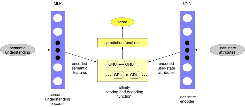
Figure 3: Dual Encoder, Affinity Decoder Topology used on the internal dataset. Input features are grouped into two categories: semantic understanding and user-state attributes. The former is fed into a Multi-Layer Perceptron (MLP) encoder, and the latter to a CNN encoder. The resulting encoded states are used in the Affinity Decoder where the decoded states are used in the prediction function to produce a score for the downstream tasks (classification, ranking, etc). For AwA2 dataset we use image features in the place of semantic features, and numeric attributes in the place of user-state attributes.

$$G1_{t}=\sigma(W_{G1}\cdot[h_{t-1},x_{t}])$$ (8)

$$G2_{t}=\sigma(W_{G2}\cdot[h_{t-1},x_{t}])$$ (9)

The candidate and actual hidden states are computed as:

$$\widetilde{h_{t}}=\tanh(W\cdot[G2_{t}*h_{t-1},x_{t}])$$ (10)

$$h_{t}=(1-G1_{t})*h_{t-1}+G1_{t}*\widetilde{h_{t}}$$ (11)

The model trained with this architecture, hidden-state initialization and update procedure outperforms other architectures both with/without meta-learning the optimizer in few-shot tasks as shown in Table 1 and Table 4.

5 Experiments

5.1 Datasets

We empirically evaluate our approach on one internal dataset and three benchmark datasets for the task of few-shot learning.

5.1.1 Internal Data

Our internal dataset consists of 10,000 user requests to a voice assistant from six domains: music, videos, app-launch, and three knowledge-related domains. This dataset consists of all the features for intents from the suite of models from Speech Recognition and Natural Language Understanding (NLU) components. All data is anonymized and minimal information leaves the user’s device.

Each request has a corresponding list of intents generated by the Speech and NLU components. Every intent has certain attribute values extracted from user-data. We have 110 such attributes for these six domains of both categorical and numeric types. These attributes capture the relevance and executability aspects whereas features from Speech and NLU components capture the semantic-understanding aspects. Each intent for a user-request is assigned with a relevance grade internally by our annotators.

We created 5 different combinations of the dataset where for each combination we had 3 training domains, 1 validation domain and 2 test domains. Every domain had 5-data points in training, 15 in both validation and test that are randomly sampled without replacement.

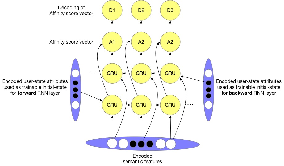
Figure 4: Affinity Decoder. Encodings for semantic features and user-state attributes are obtained using two different encoders. A bidirectional GRU layer is used in the affinity decoder. The initial hidden states of this layer are initialized using user-state attributes encoding, and the GRU cell unfolds on the semantic feature encoding sequence. The hidden states of the GRU layer are made trainable while restricting the update to only within the decoder and not propagating until the encoder’s parameters. The affinity score vector (GRU layer output) is propagated to a linear layer to produce the decoder states.

5.1.2 Microsoft MQ2007

The MQ2007 is one of the two query sets from LETOR (LEarning TO Rank) benchmark datasets. The specific dataset we used is from LETOR 4.0 (Qin & Liu, 2009) and consists of 1,700 queries with standard features, relevance labels. Since there is no concept of domains/classes in this dataset, we performed K-means clustering for K=10, we chose K by performing Silhouette analysis with threshold for the measure at 0.5. We created 5 different combinations of the dataset where each combination had 5 training domains, 2 validation domains and 3 test domains. Every domain had 5 data-points in training. Validation and test had 15 data-points that were randomly sampled without replacement.

5.1.3 Mini-ImageNet

The Mini-ImageNet dataset was originally proposed by (Vinyals et al., 2016), since exact splits were not released then, (Ravi & Larochelle, 2017) introduced new procedure with 100 classes. We follow their procedure of selecting random 100 classes: 64 training classes, 16 validation classes and 20 test classes to directly compare with their performance. We use 5 examples per class in training and 15 examples per class both in validation and test to perform 5-shot classification.

5.1.4 Animals with Attributes 2 (AwA2)

Animals with Attributes 2 (Xian et al., 2018) is a widely-used benchmark dataset for transfer learning algorithms. It consists of 37,322 images with 50 classes and 85 numeric attribute values for each class. This dataset share similar characteristics with our internal dataset having separate attribute features. We created 5 different combinations of the dataset with each combination having 30 training classes, 5 validation classes and 15 test classes. We randomly sampled 5 examples from proposed split (Xian et al., 2018) for training and 15 examples for validation and testing each, per class.

5.2 Training Details

For all the gradient-based methods we used the same hyperparameter tuning strategy which is a combination of grid and random search, and Adam optimizer with default parameters. We employed exponential decay for the learning-rate schedule. The exploration probability, $p_{explore}$, used in GRE-METL was grid-searched with a step-size of 0.1 in the range [0.0, 1.0]. The results were sensitive to the value of $p_{explore}$. On MQ2007 and Mini-ImageNet the optimal $p_{explore}$ values were 0.3 and 0.4 respectively, whereas on our internal dataset and AwA2 the optimal $p_{explore}$ value was 0.1.

For the internal and AwA2 datasets we trained a ranker and a classifier respectively using GRE-METL and encoder-decoder architecture as described in Algorithm 2, Section 3 and Section 4. For training LambdaMART (Burges, 2010) we used XGBoost implementation. Meta-LSTM (Ravi & Larochelle, 2017) was trained using the Torch implementation. We used pairwise ranking loss for training ranker models and categorical cross-entropy for classifier models. MAML (Finn et al., 2017a) was trained using the TensorFlow implementation. For training LambdaMART with MAML, we modified the parameter update to use lambda (Burges et al., 2006) computed using the $1^{st}$ order derivative of the loss function instead of the originally proposed method of using gradient obtained through gradient. Prototypical Networks were trained using PyTorch implementation.

Our encoder-decoder architecture was only used on our internal and AwA2 datasets since they share similar characteristics that can be leveraged in our proposed architecture, i.e., having different feature groups.

6 Results

Our primary results are summarized in Tables 1, 2, 3, and 4. $\pm$ denotes a 99% confidence interval.

6.1 Internal Data

Although we have relevance grades for the intents and we use LTR (Learning to Rank) to choose the best intent, unlike in traditional LTR problems, the top intent in the ranked intent list could be especially important, such as for some assistant contexts where giving only one result may be necessary. Hence we use the top intent accuracy as our metric. We show significant improvements over other techniques that are SOTA (state-of-the-art) on comparable tasks both with and without meta-learning using our encoder-decoder architecture. Table 1 shows the accuracy mean and 3-$\sigma$ (3 standard deviations) of the 5 different dataset combinations for 5-shot training along with standard deviation. For brevity we refer to our encoder-decoder architecture as DEnc-ADec.

Table 1: Evaluation results of the internal dataset with mean-accuracy and 99% confidence intervals. All results in italics use one or both of Dual-Encoder, Affinity Decoder architecture or/and GRE-METL algorithm.

Algorithm	Top Intent Accuracy (5-shot)
Logistic Regression	34.1% $\pm$ 0.3%
Feed Forward 3-layer NN	34.3% $\pm$ 0.7%
Hyp-Rank	38.2% $\pm$ 2.3%
LambdaMART	43.7% $\pm$ 0.1%
DEnc-ADec	45.6% $\pm$ 1.2%
Meta-LSTM w/ DEnc-ADec	54.2% $\pm$ 0.6%
GRE-METL w/ LambdaMART	57.3% $\pm$ 1.4%
MAML with DEnc-ADec	61.4% $\pm$ 0.9%
GRE-METL w/ DEnc-ADec	65.1% $\pm$ 1.5%

6.2 Microsoft MQ2007

On MQ2007 dataset we trained ranking models on the 5 different dataset combinations for 10-way, 5-shot ranking task. We use NDCG (Normalized Discounted Cumulative Gain) as our metric and we show significant improvements over SOTA approaches on both NDCG@1 and NDCG@5, shown in Table 2.

Table 2: Evaluation results of the MQ2007 dataset.

Algorithm	Test NDCG@1 (5-shot)	Test NDCG@5 (5-shot)
LambdaMART	67% $\pm$ 0.2%	71% $\pm$ 0.1%
Meta-LSTM w/ LambdaMART	52% $\pm$ 4.5%	56% $\pm$ 1.8%
MAML w/ LambdaMART	54% $\pm$ 3.2%	73% $\pm$ 1.7%
GRE-METL w/ LambdaMART	73% $\pm$ 2%	81% $\pm$ 2.5%

6.3 Mini-ImageNet

We trained ResNet classifier as our baseline and improved it with other meta-learning approaches including ours, we also trained Prototypical Networks (Snell et al., 2017). We report 5-shot classification accuracies on this dataset, shown in Table 3. We significantly outperform all existing approaches, and perform slightly better than Prototypical Networks.

Table 3: Evaluation results of the Mini-ImageNet dataset.

Algorithm	Classification Accuracy (5-shot)
Baseline ResNet	52% $\pm$ 1.4%
Meta-LSTM w/ ResNet	61.2% $\pm$ 0.8%
MAML w/ ResNet	63.1% $\pm$ 0.4%
Prototypical Networks	69.4% $\pm$ 0.8%
GRE-METL w/ ResNet	71.10% $\pm$ 1.7%

6.4 Animals with Attributes 2 (AwA2)

For AwA2 dataset we trained baseline ResNet and improved it with meta-learning algorithms. We also trained Prototypical Networks. Our encoder-decoder architecture combined with meta-learning specifically with GRE-METL shows significant improvements in Table 4 on 5-shot accuracies.

Table 4: Evaluation results of the AwA2 dataset.

Algorithm	Classification Accuracy (5-shot)
Baseline ResNet	37.4% $\pm$ 2.7%
Meta-LSTM w/ ResNet	47.8% $\pm$ 0.8%
MAML w/ ResNet	57.2% $\pm$ 1.3%
Prototypical Networks	66.4% $\pm$ 0.6%
GRE-METL w/ ResNet	67.5% $\pm$ 0.5%
GRE-METL w/ DEnc-ADec	70.2% $\pm$ 1.3%

7 Conclusion

We introduced a novel, generic, and flexible meta-learning scheme for few-shot learning based on the idea that we can learn the optimization algorithm by implicitly transforming the loss surface while retaining the general properties. We also showed how the framework is easily extended to perform network architecture search. We empirically show our approach sets new state-of-the-art on AwA2 and MQ2007 datasets and achieves comparable results with Prototypical Networks on Mini-ImageNet.

8 Future Work

While the current approaches including the proposed method achieve good performance on the desired evaluation metrics, it is not clear how to add a compactness metric as a reward along with the desired evaluation metric. To have a more practical reach and impact of these models it is important to deploy them on-device. This also helps preserve user-privacy and improve latency by saving round-trips to the server. Hence it is necessary to build compact models that can run on the device, especially the ones with limited compute resources. We plan to investigate how to achieve the desired compactness characteristic of the model with minimal or no drop in the model performance.

References

- Andrychowicz et al. (2016) Andrychowicz, M., Denil, M., Gomez, S., Hoffman, M. W., Pfau, D., Schaul, T., and de Freitas, N. Learning to learn by gradient descent by gradient descent. Neural Information Processing Systems, 2016.
- Baxter et al. (1995) Baxter, J., Caruana, R., Mitchell, T., Pratt, L. Y., Silver, D. L., and Thrun, S. Knowledge consolidation and transfer in inductive systems. NIPS 1995 workshop on learning to learn, 1995.
- Baydin et al. (2017) Baydin, A. G., Cornish, R., Rubio, D. M., Schmidt, M., and Wood, F. D. Online learning rate adaptation with hypergradient descent. CoRR, abs/1703.04782, 2017.
- Bengio et al. (1992) Bengio, S., Bengio, Y., Cloutier, J., and Gecsei, J. On the optimization of a synaptic learning rule. Optimality in Artificial and Biological Neural Networks, 1992.
- Bengio et al. (1990) Bengio, Y., Bengio, S., and Cloutier, J. Learning a synaptic learning rule. Universite de Montreal, Departement dinformatique et de recherche operationnelle, 1990.
- Brazdil et al. (1998) Brazdil, P., Carrier, C. G., Soares, C., and Vilalta, R. Lifelong learning algorithms. Springer, 1998.
- Brazdil et al. (2008) Brazdil, P., Carrier, C. G., Soares, C., and Vilalta, R. Metalearning: applications to data mining. Springer Science and Business Media, 2008.
- Burges (2010) Burges, C. J. From ranknet to lambdarank to lambdamart: An overview. Microsoft Research Technical Report MSR-TR-2010-82, 2010.
- Burges et al. (2006) Burges, C. J., Ragno, R., and Le, Q. V. Learning to rank with nonsmooth cost functions. Advances in Neural Information Processing Systems, 2006.
- Byrd et al. (2016) Byrd, R. H., Hansen, S. L., Nocedal, J., and Singer, Y. A stochastic quasi-newton method for large-scale optimization. SIAM Journal on Optimization, 26(2):1008–1031, 2016.
- Cho et al. (2014) Cho, K., van Merrienboer, B., Gulcehre, C., Bahdanau, D., Bougares, F., Schwenk, H., and Bengio, Y. Learning phrase representations using rnn encoder–decoder for statistical machine translation. arXiv:1406.1078, 2014.
- Duan et al. (2016) Duan, Y., Schulman, J., Chen, X., Bartlett, P. L., Sutskever, I., and Abbeel, P. Rl2: Fast reinforcement learning via slow reinforcement learning. arXiv:1611.02779, 2016.
- Duchi et al. (2011) Duchi, J., Hazan, E., and Singer, Y. Adaptive subgradient methods for online learning and stochastic optimization. 2011.
- Finn et al. (2017a) Finn, C., Abbeel, P., and Levine, S. Model-agnostic meta-learning for fast adaptation of deep networks. arXiv:1703.03400, 2017a.
- Finn et al. (2017b) Finn, C., Yu, T., Zhang, T., Abbeel, P., and Levine, S. One-shot visual imitation learning via meta-learning. 1st Conference on Robot Learning (CoRL 2017), Mountain View, United States., 2017b. URL http://proceedings.mlr.press/v78/finn17a/finn17a.pdf?source=post_page.
- Gui et al. (2018) Gui, L.-Y., Wang, Y.-X., Ramanan, D., and Moura, J. M. F. Few-shot human motion prediction via meta-learning. Springer Nature Switzerland AG 2018, 2018. URL https://www.ri.cmu.edu/wp-content/uploads/2018/12/yuxiongw_eccv18_fewshot.pdf.
- Hochreiter & Schmidhuber (1997) Hochreiter, S. and Schmidhuber, J. Long short-term memory. Neural Computation, 9(8):1735–1780, 1997.
- Hochreiter et al. (2001) Hochreiter, S., Younger, A. S., and Conwell, P. R. Learning to learn using gradient descent. Springer, 2001.
- Kingma et al. (2014) Kingma, Diederik, and Ba, J. Adam: A method for stochastic optimization. arXiv:1412.6980, 2014.
- Koch (2015) Koch, G. Siamese neural networks for one-shot image recognition. ICML Deep Learning Workshop, 2015.
- Lake et al. (2011) Lake, B. M., Salakhutdinov, R., Gross, J., and Tenenbaum, J. B. One shot learning of simple visual concepts. In CogSci, 2011.
- Li & Malik (2016) Li, K. and Malik, J. Learning to optimize. arXiv:1606.01885, 2016.
- Miller et al. (2000) Miller, E. G., Matsakis, N. E., and Viola, P. A. Learning from one example through shared densities on transforms. In IEEE Computer Vision and Pattern Recognition, volume 1, pages 464–471, 2000.
- Qin & Liu (2009) Qin, T. and Liu, T.-Y. Introducing letor 4.0 datasets. arXiv preprint arXiv:1306.2597, 2009.
- Ravi & Larochelle (2017) Ravi, S. and Larochelle, H. Optimization as a model for few-shot learning. ICLR, 2017.
- Recht & Rahimi (2017) Recht, B. and Rahimi, A. Reflections on random kitchen sinks. 2017. URL http://www.argmin.net/2017/12/05/kitchen-sinks.
- Rolinek & Martius (2016) Rolinek, M. and Martius, G. L4: Practical loss-based stepsize adaption for deep learning. arXiv:1802.05074, 2016.
- Santoro et al. (2016) Santoro, A., Bartunov, S., Gomez, S., Botvinick, M., Wierstra, D., and Lillicrap, T. P. One-shot learning with memory-augmented neural networks. CoRR, abs/1605.06065, 2016.
- Schmidhuber (1990) Schmidhuber, J. Learning to control fast-weight memories. Neural Computation, 1990.
- Snell et al. (2017) Snell, J., Swersky, K., and Zemel, R. Prototypical networks for few-shot learning. Neural Information Processing Systems, 2017.
- Thrun & Pratt (2012) Thrun, S. and Pratt, L. Learning to learn. Springer Science and Business Media, 2012.
- Tieleman & Hinton (2012) Tieleman, T. and Hinton, G. Lecture 6.5- rmsprop: Divide the gradient by a running average of its recent magnitude. COURSERA: Neural networks for machine learning, 2012.
- Vilalta & Drissi (2002) Vilalta, R. and Drissi, Y. A perspective view and survey of meta-learning. Artificial Intelligence Review, 2002.
- Vinyals et al. (2016) Vinyals, O., Blundell, C., Lillicrap, T., Wierstra, D., and et al. Matching networks for one shot learning. Neural Information Processing Systems, 2016.
- Wang et al. (2016) Wang, J. X., Kurth-Nelson, Z., Tirumala, D., Leibo, J. Z., Munos, R., Blundell, C., Kumaran, D., and Botvinick, M. Learning to reinforcement learn. arXiv:1611.05763, 2016.
- Williams (1992) Williams, R. J. Simple statistical gradient-following algorithms for connectionist reinforcement learning. Machine learning, 8(3-4):229–256, 1992.
- Xian et al. (2018) Xian, Y., Lampert, H. C., Schiele, B., and Akata, Z. Zero-shot learning - a comprehensive evaluation of the good, the bad and the ugly. TPAMI, 2018.
- Xu et al. (2018) Xu, Z., Tang, C., and Tomizuka, M. Zero-shot deep reinforcement learning driving policy transfer for autonomous vehicles based on robust control. IEEE ITSC 2018, 2018. URL https://arxiv.org/abs/1812.03216.
- Zoph & Le (2017) Zoph, B. and Le, Q. V. Neural architecture search with reinforcement learning. arXiv:1611.01578, 2017.