Probabilistic Analysis of rrt Trees

Abstract

This thesis presents analysis of the properties and run-time of the Rapidly-exploring Random Tree (rrt) algorithm. It is shown that the time for the rrt with stepsize $\epsilon$ to grow close to every point in the $d$-dimensional unit cube is $\Theta\left(\frac{1}{\epsilon^{d}}\log\left(\frac{1}{\epsilon}\right)\right)$. Also, the time it takes for the tree to reach a region of positive probability is $O\left(\epsilon^{-\frac{3}{2}}\right)$. Finally, a relationship is shown to the Nearest Neighbour Tree (nnt). This relationship shows that the total Euclidean path length after $n$ steps is $O(\sqrt{n})$ and the expected height of the tree is bounded above by $(e+o(1))\log n$.

Figure 1: The growth of the rrt at times $\Theta\left(\frac{1}{\epsilon}\right)$ left and $\Theta\left(\frac{1}{\epsilon^{2}}\right)$ right. Above the rrt is expanding outwards quickly. Below the rrt has begun to fill holes left by its expansion but is far from covering the space.

1 Introduction

In 1998, LaValle [12] introduced a ground-breaking approach to path planning: the Rapidly-exploring Random Tree (rrt). At the time the area of path planning had already been taken over by randomized algorithms due to strong evidence of a limit on the potential speed of deterministic path [11, 16, 15]. The rrt was a novel randomized approach that has quickly come to dominate modern path planning. Previously the most widely used algorithm had been the probabilistic road map [10, 3], an algorithm which randomly selects points in the space and connects these points to the graph. The rrt differed, in that rather than adding these randomly selected points, it built a tree with small edge length based on these points.

The rrt’s ubiquity is in large part due to a number of variants to the original algorithm, such as the rrt-Connect [11, 13] and the rrt* [9, 8]. In the former, we grow an rrt out of both the initial and final point of a desired path, while trying to connect them. In the latter, to optimize the spanning ratio we grow our tree based on a choice of minimal path length as well as the locations of the randomly selected points. These modifications and others are missing analytical grounding to understand their performance.

There have been prior analyses of the rrt but none in quite this area. Soon after the creation of the rrt, Kuffner and LaValle [11] proved that the algorithm was probabilistically complete—i.e., the algorithm succeeds with high probability—and that the distribution of the $n$-th vertex in the tree converges to the sampling distribution. In their analysis however, they commented that they had no result on the speed of this convergence. Further analysis has been done by Arnold et al. [1] on the speed at which the rrt spreads out by studying an idealized version of the algorithm on an infinite disc. Work has also been done by Karaman and Frazzoli [9] on the complexity of the update step in the algorithm and the optimality of the path, while Dalibard and Laumond [3] have studied the effects of narrow passages on the performance of the algorithm. However there remains a gap in the literature on determining a run time until success of the rrt. This paper aims to fill this gap.

1.1 Organization

The paper is organized as follows: first we set out definitions and a framework for our approach. We then split our analysis into three phases of growth of the rrt.

The first phase is the phase where the rrt spreads out quickly. Most of the space is still far away from the tree, so most steps give a large amount of progress. This is the phase most similar to the problem considered by Arnold et al.[1].

The second phase is the phase where the rrt grows close to every point in the space. Kuffner and LaValle [11] proved that this occurs and we will add information on the speed.

Finally, the third phase covers the growth of the tree once the rrt has grown close to every point in the graph. We find a relationship here to the nearest neighbour tree which allows easy study of the tree and many results on its behaviour.

2 Definitions

2.1 Initial Framework

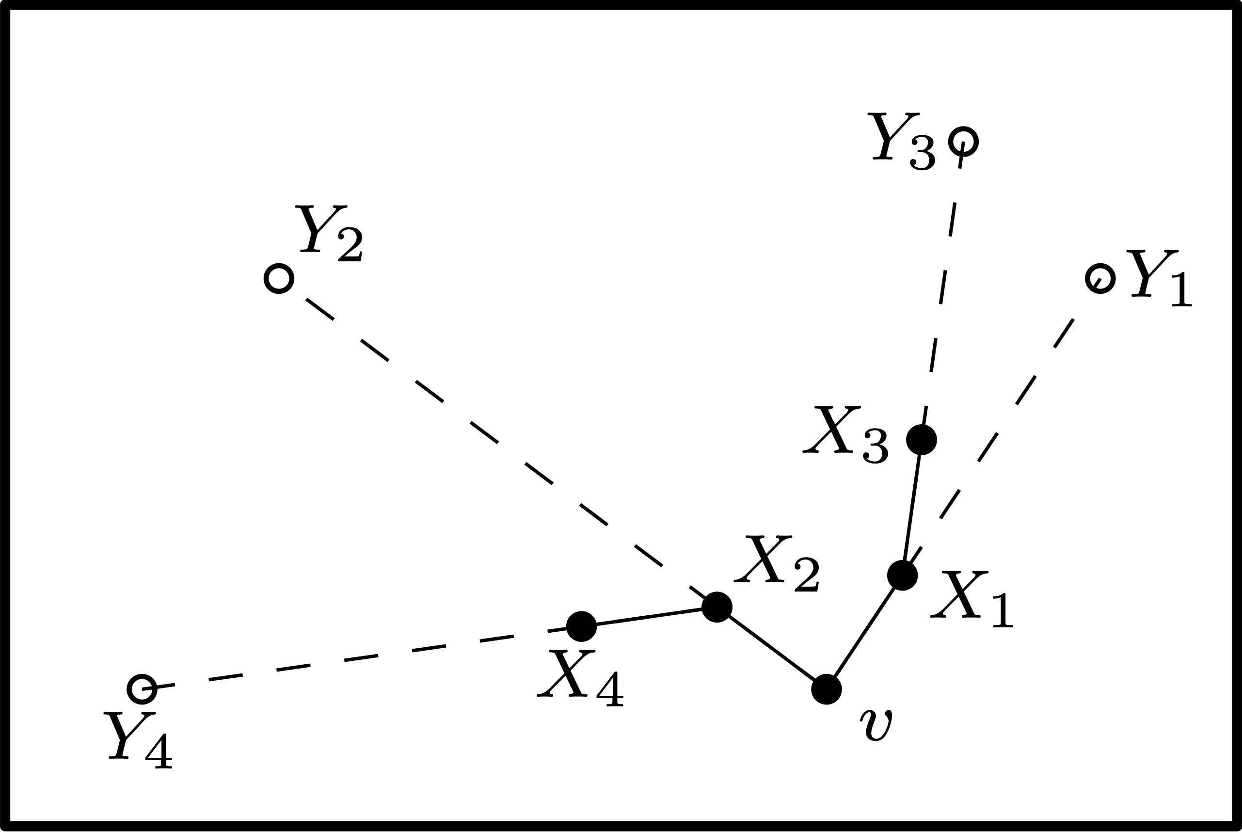
Figure 2: The start of an rrt. The $X_{i}$’s are the vertices and the $Y_{i}$’s are their determining uniform random variables.

We begin with basic definitions of the rrt on compact, convex metric spaces. In lieu of the vocabulary used in general path planning problems, we will use the vocabulary of metric spaces and probability.

Definition 1.

An rrt is a sequence of vertex and edge random variable pairs

$$T_{\epsilon}(M,v):=((X_{i},E_{i}))_{i\in\mathbb{N}}$$

defined on a compact metric space $M$ with distance function $d$, a step-size parameter $\epsilon>0$, $E_{0}=\emptyset$, and an initial vertex $v=X_{0}\in M$. Each $(X_{i},E_{i}),i\geq 1$ is generated in the following way: take a sequence of uniform $M$-valued random variables $(Y_{i})_{i=1}^{\infty}$ and let

$$\gamma_{i}=\textnormal{argmin}_{0\leq j\leq i-1}d(Y_{i},X_{j}).$$

Define

$$X_{i} :=\begin{cases}Y_{i}&:\text{if}\ \min_{0\leq j\leq i-1}d(x_{i},v_{j})\leq\epsilon,\\ X_{\gamma_{i}}+\epsilon\frac{Y_{i}-X_{\gamma_{i}}}{d(Y_{i},X_{\gamma_{i}})}&:\textnormal{otherwise},\end{cases}$$

and

$$E_{i} :=(X_{\gamma_{i}},X_{i}).$$

An rrt at time $n\in\mathbb{N}$ is the subset $T_{\epsilon}^{n}(M,v)\subset T_{\epsilon}(M,v)$ given by

$$T_{\epsilon}^{n}(M,v):=((X_{i},E_{i}))_{1\leq i\leq n}.$$

In plain terms, we start with an initial vertex $v$ and then iteratively we select a point $Y_{i}$ uniformly in the space, find $X_{\gamma_{i}}$—the closest vertex in the tree at time $i-1$—and then add a vertex-edge pair in the direction of $Y_{i}$ with edge length less than or equal to $\epsilon$. In this definition we do not check for obstacles blocking the edge as we are assuming the space to be convex.

To remove clunkiness in notation, we often leave $M$ and $v$ implicit and just write $T_{\epsilon}^{n}$. Typically, $M$ will be the $d$-dimensional unit cube $[0,1]^{d}$. Also, the initial vertex $v$ is often irrelevant to our analysis.

2.2 Covering Metric Spaces

One measure of success for the rrt is whether or not the tree has grown close to every point in the space. A natural definition for “close” for an rrt $T_{\epsilon}^{n}$ is being within $\epsilon$ of the tree.

Definition 2.

Consider a compact metric space $M$ and a graph $G=(V,E)\subset M$ where $V$ is the set of vertices and $E$ is the set of edges. The $\epsilon$-cover of $G$ is

$$C_{\epsilon}(G):=\bigcup_{v\in V}B(v,\epsilon)$$

where $B(x,\epsilon)$ is the ball

$$B(x,\epsilon)=\left\{y\in M:d(x,y)\leq\epsilon\right\}.$$

In the case of an rrt $T_{\epsilon}^{n}=((X_{i},E_{i}))_{1\leq i\leq n}$, the cover is

$$C(T_{\epsilon}^{n}):=\bigcup_{0\leq i\leq n}B(X_{i},\epsilon).$$

Definition 3.

The covering time of a metric space $M$ by an rrt $T_{\epsilon}^{n}$ is the $\mathbb{N}$-valued random variable

$$\tau(T_{\epsilon})=\min\{n\in\mathbb{N}:C(T_{\epsilon}^{n})\supset M\}.$$

In particular, we will analyze the expected covering time, $\mathbb{E}\left[\tau(T_{\epsilon})\right]$. Unless explicitly noted, we assume that $M=[0,1]^{2}$.s

3 Phase 1—Initial Growth

Figure 3: The first phase of an rrt.

We begin by studying how quickly the rrt spreads. Arnold et al. [1] consider a modification to the rrt where the space is the plane $\mathbb{R}^{2}$, the step size is 1, and points are drawn at infinity by picking a ray from the origin with a uniformly random direction. They prove in this model that the perimeter of the convex hull of tree grows linearly in time which implies that the maximum distance from the tree to the origin also grows linearly in time. Here, we consider a related question: how long does it take an rrt to reach a convex region of positive probability?

While a number of such regions can be chosen, for ease of calculation we consider the case that we have an rrt on $[0,1]^{2}$ and the region we want to reach is the right half of the square, $\left[\frac{1}{2},1\right]\times[0,1]$ when $X_{0}=(0,0).$ Similar arguments extend to the general convex region.

Theorem 1.

For an rrt $T_{\epsilon}$ on $[0,1]^{2}$, the expected time to reach $\left[\frac{1}{2},1\right]\times[0,1]$ is $O\left(\epsilon^{-\frac{3}{2}}\right)$ as $\epsilon\to 0$.

Proof.

We will follow the vertex with greatest $x$-value through the whole process. Consider the Voronoi region of this point. There are two cases: either there are multiple vertices with the same $x$-value or there is a single vertex with greatest $x$-value. If there are multiple vertices with the same $x$-value then then we have a greater chance of useful progression so we focus on the case of a unique vertex.

Suppose we have a unique vertex with greatest $x$-value, $v$. Consider any other vertex in the tree, $w$. This vertex only impacts the Voronoi region of $v$ by the perpendicular bisector of the line between $v$ and $w.$ Following this, we look at where $v$’s Voronoi region intersects the right edge of the box, $\{1\}\times[0,1]$ and see that it does so at the edge of the Voronoi region of some other vertex. Also, we see that the Voronoi region contains a triangle from the vertex $v$ to the intersections of its Voronoi region with $\{1\}\times[0,1]$.

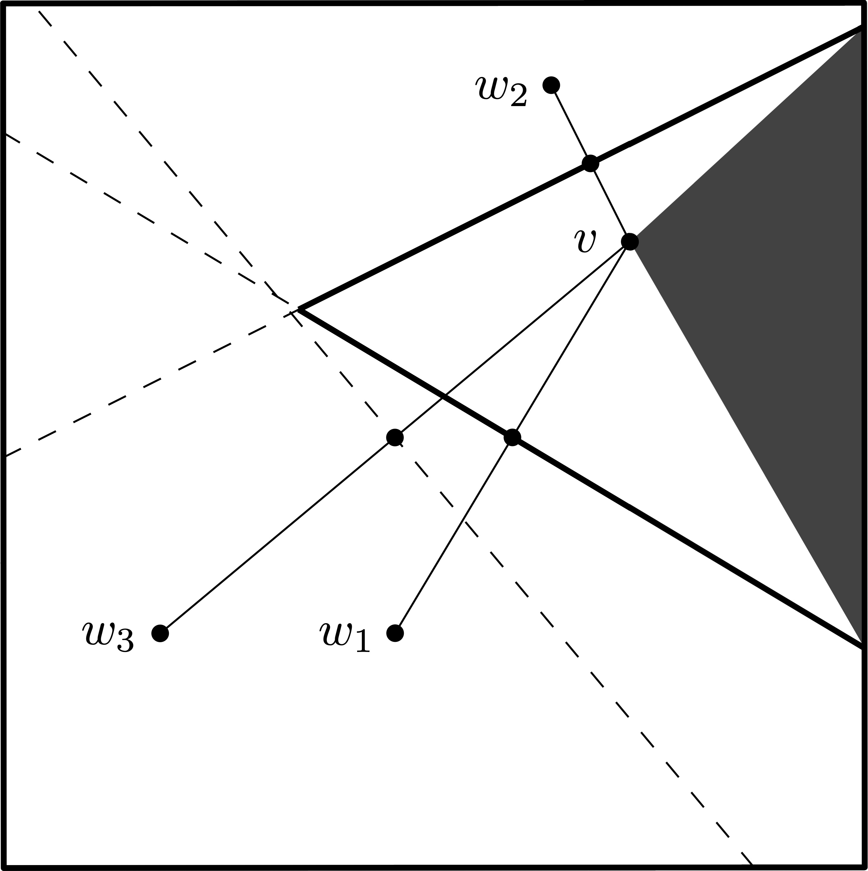
Figure 4: The Voronoi region of $v$ made of its pairwise Voronoi regions.

Our goal is to find a probability of progress which we will do by looking at this triangle—more specifically by considering triangles and considering when the Voronoi region would contain this triangle. In the worst case scenario, $v$ is on the upper or lower edge of $[0,1]^{2}$, so without loss of generality, we take $v$ to be on the upper edge.

Consider the triangle $\Lambda$ with points $v,(1,1),$ and $(1,1-\delta)$ for some $\delta>0$. The first question to ask is when will the Voronoi region of $v$ not contain $\Lambda$? We find the region where any vertex other that $v$ inside will have a Voronoi region intersecting $\Lambda$. Observe that for any point $w$ on the boundary of this region, the perpendicular bisector of the line between $v$ and $w$ must pass through $(1,1-\delta)$. Writing

$$w=v-(x,y)=(1-z-x,1-y),$$

consider the similar triangles

$$\left\{v,v-\left(\frac{x}{2},\frac{y}{2}\right),v-\left(0,\frac{y}{2}\right)\right\}$$

and

$$\left\{(1,1-\delta),\left(1,1-\frac{y}{2}\right),v-\left(\frac{x}{2},\frac{y}{2}\right)\right\}.$$

We have the equality

$$\frac{x}{y}=\frac{\delta-\frac{y}{2}}{z+\frac{x}{2}},$$

which implies that the boundary points $w=(x_{0},y_{0})$ all lie on the circle $\mathcal{C}$ whose points satisfy

$$\left(x+z\right)^{2}+\left(y-\delta\right)^{2}$$

$$=\ \left(x_{0}-1\right)^{2}+(y_{0}-1+\delta)^{2}$$

$$=\ \delta^{2}+z^{2},$$

which is the circle centered at $(1,1-\delta)$ with radius $\sqrt{\delta^{2}+z^{2}}$.

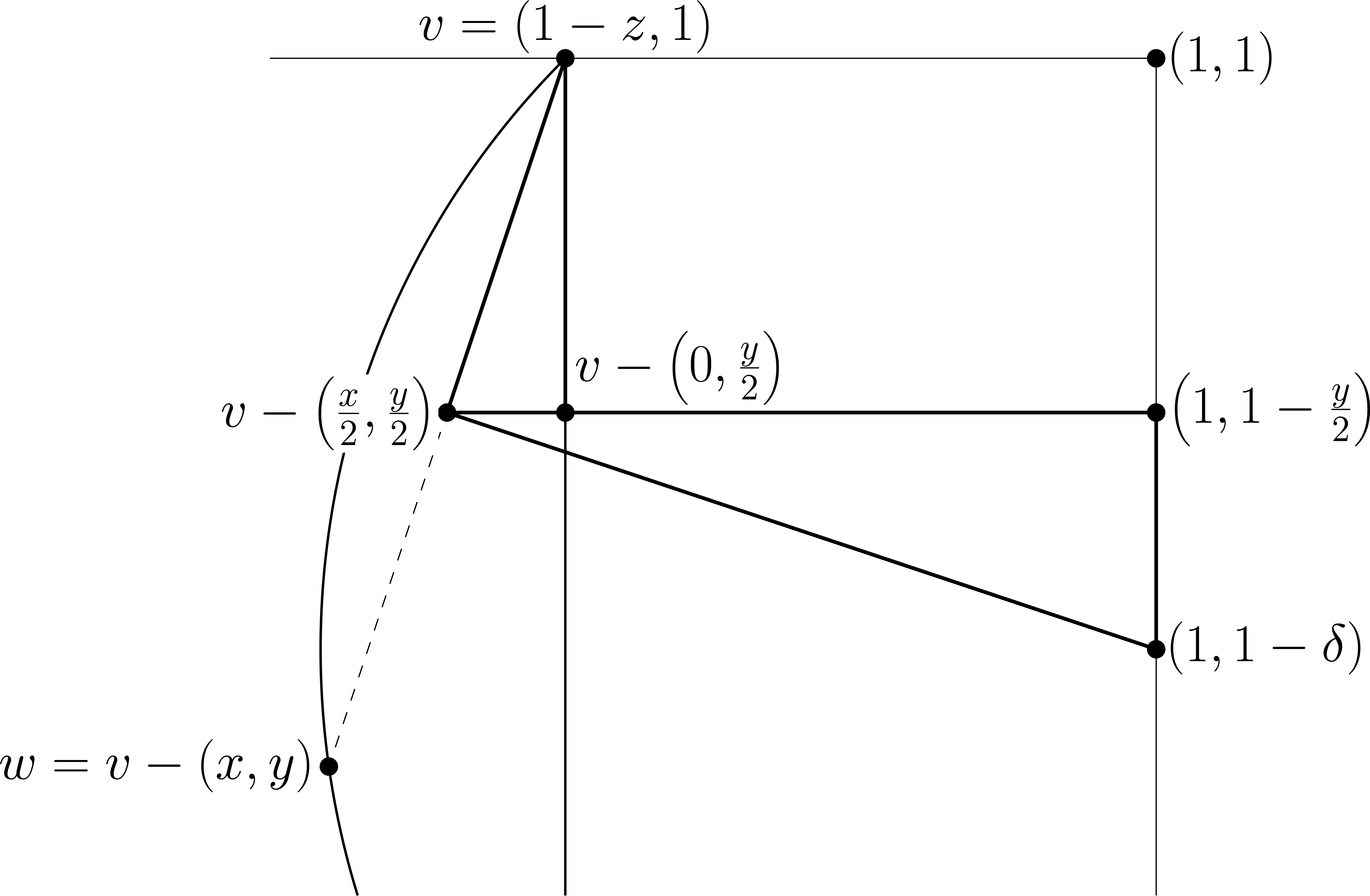
Figure 5: The similar triangles $\left\{v,v-\left(\frac{x}{2},\frac{y}{2}\right),v-\left(0,\frac{y}{2}\right)\right\}$ and $\left\{(1,1-\delta),\left(1,1-\frac{y}{2}\right),v-\left(\frac{x}{2},\frac{y}{2}\right)\right\}$.

The area that could interfere with this circle is then a cap with height

$$h(\delta,z)=\sqrt{\delta^{2}+z^{2}}-z.$$

Note that $\frac{1}{2}\leq z\leq 1$, and that $h(\delta)$ is decreasing in $z$, so we may upper bound $h(\delta,z)$ with

$$h(\delta,z)\leq\sqrt{\delta^{2}+\frac{1}{4}}:=h(\delta).$$

Now we pick $\delta$ in such a way that any time we select a point in $\Lambda$ we make $\Theta(\epsilon)$ progress. Set $\delta=\frac{1}{2}\sqrt{\epsilon}$ and take $\epsilon<\frac{1}{16}$. Suppose our $i$-th uniform vertex $Y_{i}\in\Lambda$. The easy case is that $X_{\gamma_{i}}=v$ in which case we make progress of at least $\frac{1}{\sqrt{2}}\epsilon.$ The more subtle case is if $v\not=X_{\gamma_{i}}$. Then $X_{\gamma_{i}}$ is in the circle $\mathcal{C}$ and since $v$ is the most advanced point, $X_{\gamma_{i}}$ is in fact in the cap. $X_{i}$ is at least $\frac{1}{\sqrt{2}}\epsilon$ further than $X_{\gamma_{i}}$, but how much progress have we actually made? We must analyse the difference between the height of the cap and $Z_{i}$’s progress.

We will show that the height of the cap is less than $\frac{1}{2}\epsilon$ by a constant fraction of $\epsilon$. We derive $\frac{1}{\sqrt{2}}\epsilon-h\left(\frac{1}{2}\sqrt{\epsilon}\right)$ to get

$$\frac{d}{d\epsilon}\left(\frac{1}{\sqrt{2}}\epsilon-\sqrt{\frac{1}{4}\epsilon+\frac{1}{4}}\right)\frac{1}{\sqrt{2}}-\frac{1}{8\sqrt{\frac{1}{4}\epsilon+\frac{1}{4}}}.$$

This is increasing in $\epsilon$ and at $0$ it is $\frac{1}{\sqrt{2}}-\frac{1}{4}$, so it follows that we progress by at least $\left(\frac{1}{\sqrt{2}}-\frac{1}{2}\right)\epsilon.$

Figure 6: A vertex $w$ inside the cap whose Voronoi region cuts into $\Lambda$.

This shows that it suffices to select a point in $\Lambda$ at least $\frac{1}{\left(\frac{1}{\sqrt{2}}-\frac{1}{4}\right)\epsilon}$ times to reach the right half of the unit square. Meanwhile, the area of $\Lambda$ is at least $\frac{1}{4}\sqrt{\epsilon}$ so the expected time to select a point in $\Lambda$ is less than $\frac{4}{\sqrt{\epsilon}}$. It follows that the expected time to reach $\left[\frac{1}{2},1\right]\times[0,1]$ is less than

$$\frac{1}{\left(\frac{1}{\sqrt{2}}-\frac{1}{2}\right)\epsilon}\cdot\frac{4}{\sqrt{\epsilon}}=O\left(\epsilon^{-\frac{3}{2}}\right).$$

∎

It is worth remarking that if we repeat the analysis in $[0,1]^{d}$ and wish to reach $\left[\frac{1}{2},1\right]\times[0,1]^{d-1}$ the argument above holds with slightly different constants.

The question remains whether this upper bound is tight or not. One can imagine that in expectation either some finite number of branches shoot out rapidly towards the right half of $[0,1]^{2}$—in this case we would have in fact $\Theta(\epsilon^{-1})$—or that the tree will progress with tendrils approximately $\sqrt{\epsilon}$ apart from each other moving forward evenly—this being the $\Theta\left(\epsilon^{-\frac{3}{2}}\right)$ case. The question remains open.

4 Phase 2—Covering Times

Figure 7: An rrt shortly before covering. Some parts of the space are still uncovered, while others have begun nearest neighbour behaviour.

4.1 Covering $[0,1]^{d}$

We turn our attention to the covering time for $M=[0,1]^{d}$ in the Euclidean metric. This gives the expected run time of the algorithm to some measure of success. The following analysis does not depend on the initial vertex $v$ so we drop it. First we look at the expected covering time for an rrt on $[0,1]^{d}$.

Theorem 2.

The expected covering time of $[0,1]^{d}$ by an rrt $T_{\epsilon}$ is

$$\mathbb{E}\left[\tau(T_{\epsilon})\right]=\Theta\left(\frac{1}{\epsilon^{d}}\log\frac{1}{\epsilon}\right).$$

Proof.

We first find a lower bound for $\mathbb{E}\left[\tau(T_{\epsilon})\right]$. We consider a critical subset of the time steps: the time steps where new area is added to the cover. We work backwards from covering. Our goal is to lower bound the amount of time required for each critical step.

Define $\beta$ to be the inverse of the volume of the $d$-dimensional ball with radius $\epsilon$:

$$\beta:=\frac{\Gamma\left(\frac{d}{2}+1\right)}{\epsilon^{d}\pi^{\frac{d}{2}}},\quad\overline{\beta}:=\left\lfloor\beta\right\rfloor.$$

The maximum amount of space we cover at any critical step is $\frac{1}{\beta}$ so the number of critical steps is at least $\overline{\beta}$. As well, we will argue that the probability of achieving the $\ell$-th last critical step is bounded by $\ell\frac{2^{d}}{\beta}$.

Consider the final critical step of any rrt. The area added in this step is a possibly uncountable set of points contained in an $\epsilon$-ball. Letting $i$ be any time before the final critical step and after the penultimate critical step, we note that we may only have a critical step if $Y_{i}$ is within $\epsilon$ of an uncovered point. This implies that the set of points that could lead to a critical step is contained in a $2\epsilon$-ball.

This argument can be repeated inductively—at any time the set of points that could lead to a critical step is contained in a union of $2\epsilon$-balls. To be precise, the time taken for the $\ell$-th last critical step is lower bounded by the geometric random variable with parameter $\ell\frac{2^{d}}{\beta}$.

$$\mathbb{E}\left[\textnormal{Geo}\left(\ell\frac{2^{d}}{\beta}\right)\right]=\frac{\beta}{2^{d}}\cdot\frac{1}{\ell}.$$

It follows that the covering time can be bounded below by

$$\mathbb{E}\left[\tau(T_{\epsilon})\right]\geq\frac{\beta}{2^{d}}\sum_{\ell=1}^{\overline{\beta}}\frac{1}{\ell}.$$

This gives a bound using the $\beta$-harmonic number

$$\mathbb{E}\left[\tau(T_{\epsilon})\right] \geq\frac{\beta}{2^{d}}H_{\overline{\beta}}\sim\frac{\beta}{2^{d}}\log\beta=\Omega\left(\frac{1}{\epsilon^{d}}\log\left(\frac{1}{\epsilon}\right)\right).$$

∎

For an upper bound we consider a grid over $[0,1]^{d}$ where each grid cell is a cube has side length $\frac{\epsilon}{\sqrt{d}}$. The time required for the rrt to have a vertex in each grid cell is greater than the covering time. To find upper bound we need the following lemma to bound the time required for a new cell to have a vertex.

Lemma 1.

Let $T_{\epsilon}$ be an rrt on $[0,1]^{d}$ with an $\frac{\epsilon}{\sqrt{d}}$ grid over it. Let $S_{i}$ be the union of the cells which do not contain a vertex of $T_{\epsilon}$ at time $i-1$. Then $X_{i}\in S_{i}$ if and only if $Y_{i}\in S_{i}$.

Proof.

Suppose that at some time $i,$ the cube $Y_{i}\in S_{i}$ and $X_{i}\notin S_{i}$. Clearly $X_{i}\not=Y_{i}$ so $d(X_{\gamma_{i}},Y_{i})=\epsilon+d(X_{i},Y_{i})$. But since $X_{i}\in S_{i}^{c}$, it belongs to a cell which contains $X_{j}$ for some $j<i$. It follows that

$$d(X_{j},Y_{i}) \leq d(X_{j},X_{i})+d(X_{i},Y_{i})$$

$$<\epsilon+d(X_{i},Y_{i})$$

$$=d(X_{\gamma_{i}},Y_{i}).$$

This contradicts the definition of $X_{\gamma_{i}}$ so we have proven the claim. ∎

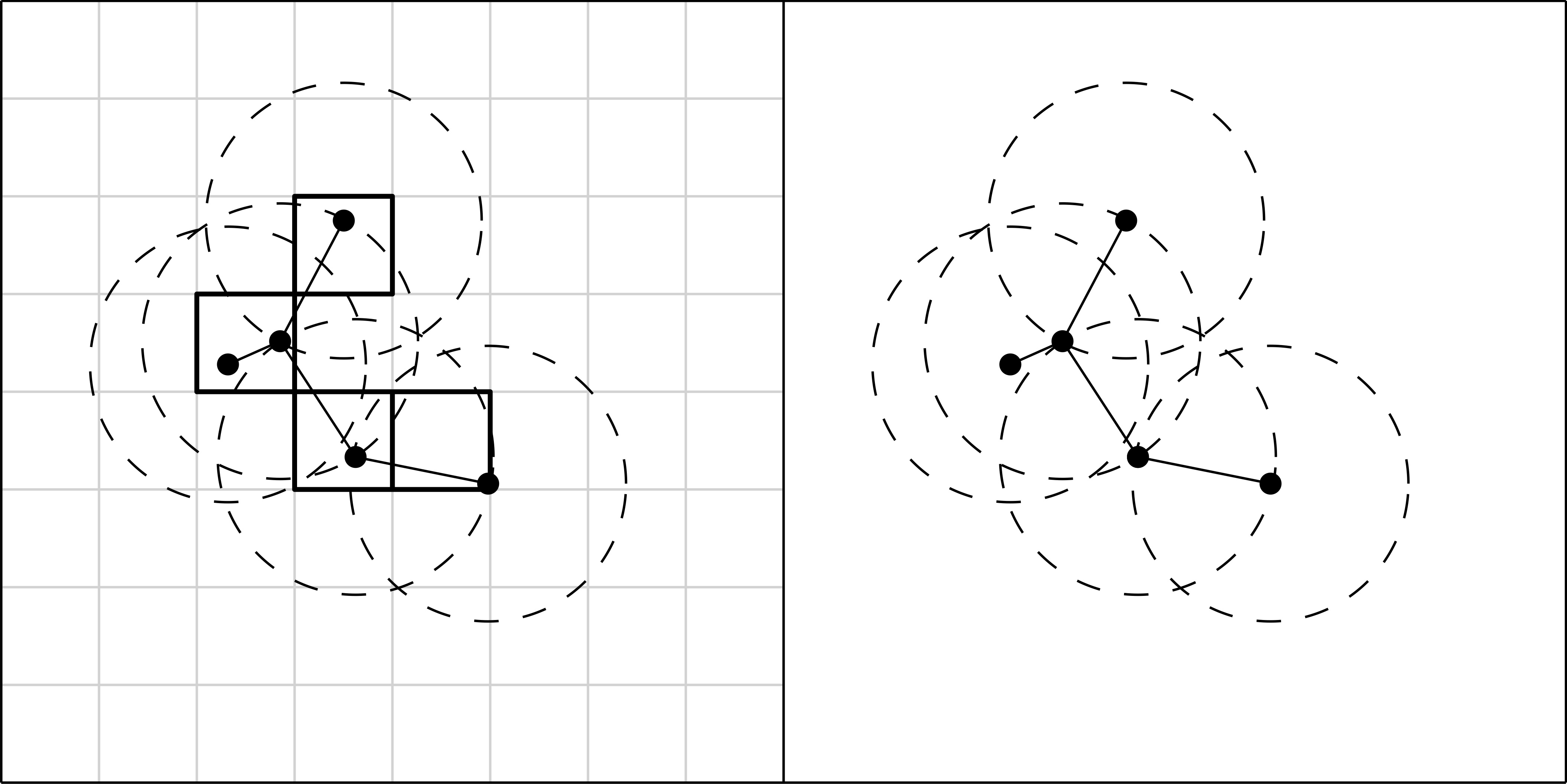
Figure 8: On the right we see a section of the rrt and the $\epsilon$-balls that it covers. On the left the space is covered with a grid and the covered sections of the grid are bolded.

Now we continue to the upper bound.

Proof.

For the $\frac{\epsilon}{\sqrt{d}}$ grid, each cell is covered by any vertex inside it. Thus the time required to have a vertex in each grid cell upper bounds $\mathbb{E}\left[\tau(T_{\epsilon})\right]$. Define $\alpha$ to be the inverse of the volume of a cell:

$$\alpha:=\frac{d^{\frac{d}{2}}}{\epsilon^{d}},\quad\overline{\alpha}=\left\lceil\alpha\right\rceil.$$

Suppose $\ell$ grid cells contain a vertex. Then, by our previous lemma, the time to add a vertex to a new cell is the time to draw a uniform random point in a new cell. This is geometric with parameter

$$\left(1-\frac{\ell}{\alpha}\right)=\left(\frac{1}{\alpha}\left(\alpha-\ell\right)\right)$$

which has expectation

$$\mathbb{E}\left[\textnormal{Geo}\left(\frac{1}{\alpha}\left(\alpha-\ell\right)\right)\right]=\frac{\alpha}{\alpha-\ell}.$$

It follows that

$$\mathbb{E}\left[\tau(T_{\epsilon})\right]\leq\alpha\sum_{\ell=1}^{\overline{\alpha}}\frac{1}{\alpha-\ell}.$$

Again, the $\alpha$-harmonic number gives an asymptotic bound

$$\mathbb{E}\left[\tau(T_{\epsilon})\right] \leq\alpha H_{\overline{\alpha}}\sim\alpha\log\alpha=O\left(\frac{1}{\epsilon^{d}}\log\left(\frac{1}{\epsilon}\right)\right).$$

Thus, we have both inequalities. ∎

Notice that this result also holds for modified rrt algorithms which maintain the property that the point drawn in an uncovered cube will cover some new cube.

As well, note that the lower and upper bounds given by this proof are asymptotically

$$\frac{\beta}{2^{d}}\log\beta =\frac{d\cdot\Gamma\left(\frac{d}{2}+1\right)}{2^{d}\pi^{\frac{d}{2}}\epsilon^{d}}\log\left(\frac{1}{\epsilon}\right)\quad+\frac{\Gamma\left(\frac{d}{2}+1\right)}{2^{d}\pi^{\frac{d}{2}}\epsilon^{d}}\log\left(\frac{\Gamma\left(\frac{d}{2}+1\right)}{\pi^{\frac{d}{2}}}\right),$$

and

$$\alpha\log\alpha=\frac{d^{\frac{d}{2}+1}}{\epsilon^{d}}\log\left(\frac{1}{\epsilon}\right)+\frac{d^{\frac{d}{2}+1}}{2\epsilon^{d}}\log d,$$

respectively.

Consider the lower bound. If we fix $\epsilon<\frac{1}{2\pi}$ and then let $d\to\infty$, the run time is $e^{\Omega(d\log d)}$, confirming that the run time is at least exponential in the dimension of the space [3].

5 Coupon Collector Problem

It is worth noticing that our upper bound argument is very similar to a classical problem. We recall the Coupon Collector Problem [14, 5]:

Theorem 3.

Suppose there exist $n$ different types of coupons and each time a coupon is drawn it is drawn independently and uniformly at random from the $n$ classes, i.e., for each coupon drawn and for each $i\in 1,..,n$ the probability that the coupon is of the $i$-th type is $\frac{1}{n}$. The expected time $T$ to have one of each type of coupon is asymptotically $n\log n$.

In our upper bound argument for the covering time of the graph we have a scenario very similar to the Coupon Collector Problem. We have divided the space into a number of cubes that we need to cover, however in our case the selection of a new cube does not guarantee that it is covered, just that some new cube is covered. In this way we see it does not matter that we are not adding the randomly selected point to our tree.

6 A Connecting Lemma—Nearest Neighbour Trees

We turn our attention to the growth of the tree after the space has been covered. From this time onward, every point of $M$ is within distance $\epsilon$ of the tree, so we will have $X_{i}=Y_{i}$ after coverage. Our analysis between the growth of the rrt in this phase depends on the relationship between the rrt and the Nearest Neighbour Tree (nnt).

Definition 4.

An nnt is a sequence of vertex and edge random variable pairs

$$T_{\textsc{nn}}=T_{\textsc{nn}}(M,v)=((X_{i},E_{i}))_{i\in\mathbb{N}}$$

defined on a compact metric space $M$ with an initial vertex $v=X_{0}$ and $E_{0}=\emptyset$. Each $(X_{i},E_{i}),i\geq 1$ is generated in the following way: take a sequence of uniform $M$-valued random variables $(X_{i})_{j=1}^{\infty}$ and let

$$\gamma_{i}=\textnormal{argmin}_{0\leq j\leq i-1}d(X_{i},X_{j}).$$

Then $X_{i}$ is added to the tree via the edge

$$E_{i}:=(X_{\gamma_{i}},X_{i}).$$ (1)

An nnt at time $n\in\mathbb{N}$ is the subset $T_{\textsc{nn}}^{n}(M,v)$ where

$$T_{\textsc{nn}}^{n}=T_{\textsc{nn}}^{n}(M,v)=((X_{i},E_{i}))_{0\leq i\leq n}.$$

Now we define a nearest neighbour process which grows onto a given tree $\Lambda$—note that $\Lambda$ may be a random tree itself. The purpose of this is to ultimately view an rrt $T_{\epsilon}$ as the growth of a nearest neighbour tree onto $T_{\epsilon}^{\tau(T_{\epsilon})},$ the rrt at covering time.

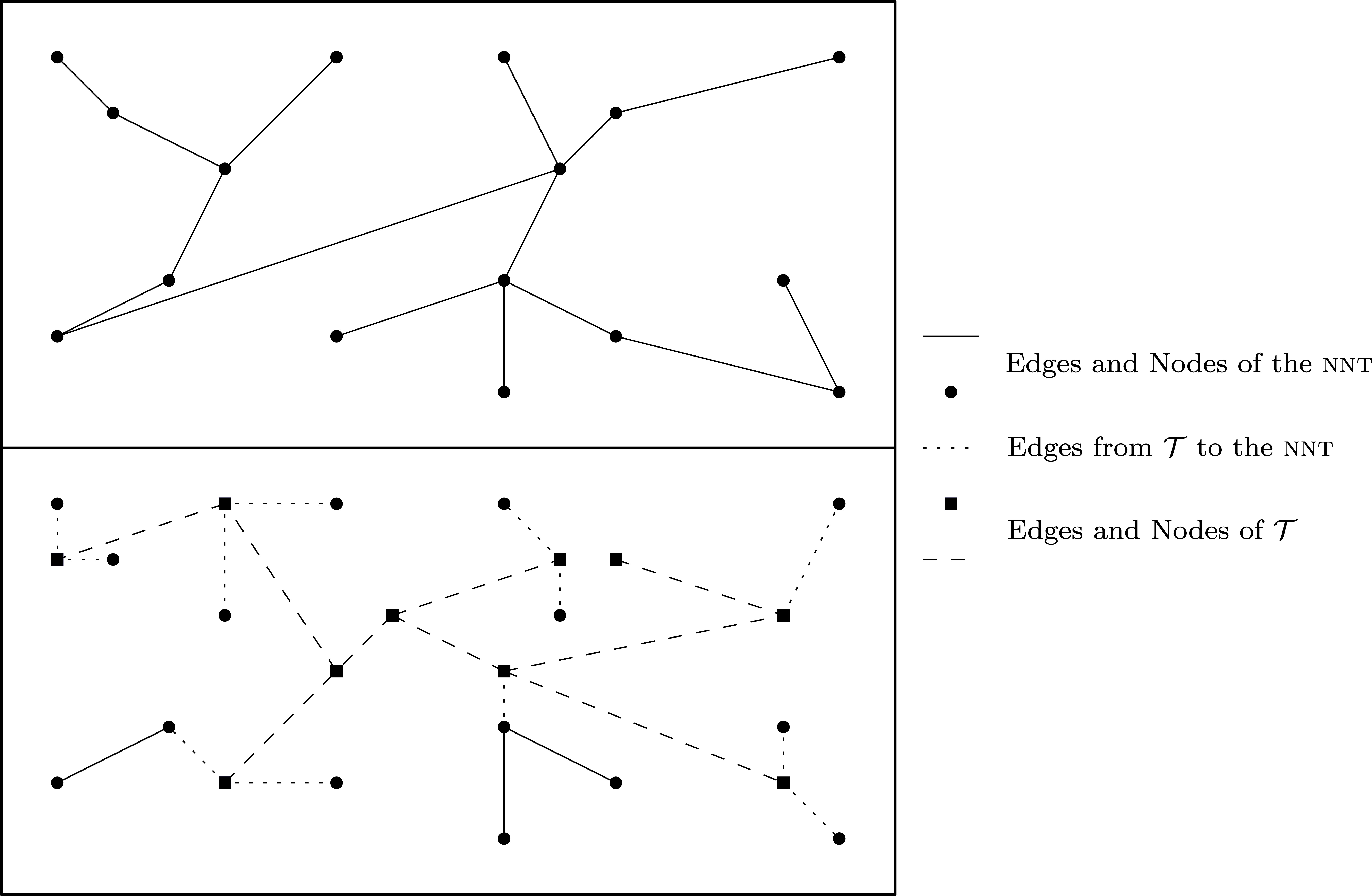
Figure 9: On top is an nnt. On the bottom is the nnt grown onto another tree $\Lambda$.

Definition 5.

Let $S$ be a random variable in $\mathbb{N}\cup\{\infty\}$ and let $\Lambda$ be a random tree embedded in a metric space $M$ with vertices $(V_{i}\in M,i\in\{0,...,S\})$ and edges $(F_{i},i\in\{1,...,S\})$. Let $T_{\textsc{nn}}=((Z_{i},E_{i}))_{i\in\mathbb{N}}$ be an nnt. The connection process of an nnt onto $\Lambda$ is the sequence of vertex and edge random variable pairs

$$T_{\Lambda}=((X_{i},E_{i}^{\prime}))_{i\in\mathbb{N}},$$

where

$$X_{i} :=\begin{cases}V_{i}&:\textnormal{if}\ 0\leq i\leq S,\\ Z_{i-M}&:\textnormal{otherwise},\end{cases}$$

$$\gamma_{i} =\textnormal{argmin}_{0\leq j\leq i-1}d(X_{i},X_{j}),$$

and

$$E_{i}^{\prime}=\begin{cases}\emptyset&:\textnormal{if}\ i=0\\ F_{i}&:\textnormal{if}\ 1\leq i\leq S,\\ (X_{i},X_{\gamma_{i}})&:\textnormal{otherwise}.\end{cases}$$

It is worth noting that the process loses a lot of meaning if $\mathbb{P}\left[S=\infty\right]\not=0$. As well, $\Lambda$ may be deterministic in which case its associated random variables are all constant.

The Connecting Lemma below links the nnt to the rrt.

Lemma 2.

Let $T_{\Lambda}=((X_{i},E_{i}^{\prime}))_{i\in\mathbb{N}}$ be the process defined above. $T_{\Lambda}$ has the following properties:

• Let $\delta_{n}$ be the distance from $Z_{n}$ to its parent in $T_{\textsc{nn}}$ and $\delta_{n}^{\prime}$ be the distance from $X_{n+S}$ to its parent in $T_{\Lambda}$. Then $\delta_{n}\geq\delta_{n}^{\prime}$.

• Let $H(\Lambda)$ be the height of $\Lambda$, $D_{n}$ be the depth of $Z_{n}$ in $T_{\textsc{nn}}$ and $D_{m}^{\prime}$ be the depth of $X_{m}$ in $T_{\Lambda}$. Then for $m=S+n$,

  $$D_{m}^{\prime}\leq D_{n}+H(\Lambda)+1.$$

Proof.

The first point follows by definition. For the second, let $m=n+M$ and let

$$\alpha=\textnormal{argmin}_{k<i\leq m}\{X_{i}:X_{i}\textnormal{ is an ancestor of }X_{m}\}.$$

The length of the path from $X_{m}$ to $X_{\alpha}$ is certainly less than $D_{n}$ and the path up the tree starting at $X_{\alpha}$’s parent is contained in $\Lambda$, so it follows that

$$D_{m}^{\prime} \leq D_{n}+D_{\alpha}^{\prime}\leq D_{n}+H(\Lambda)+1.$$

∎

Put simply, the first property of the Connecting Lemma states that the distance from a node to its parent is smaller in a connection process than an nnt. The second property states that the depth of a node in a connection process is less than the depth of the node in the nnt and an $O(H(\Lambda))$ term—importantly, in the case of the rrt $H(\Lambda)=O(1)$. Armed with this lemma, we can now analyze the behaviour of the rrt after covering.

7 Phase 3—Growth After Covering

Figure 10: An rrt well after covering time. The tree is growing denser in the space and the whole space is covered.

We first analyze the behaviour of the nnt and then relate it to the rrt via the connecting lemma. In the case of an rrt, $\Lambda=T_{\epsilon}^{\tau(T_{\epsilon})}$ and $T_{\textsc{nn}}=T_{\epsilon}-\Lambda$.

7.1 Euclidean Distances

Let $\textnormal{Exp}(\lambda)$ be a random variable $X$ with distribution

$$\mathbb{P}\left[X\leq x\right]=1-e^{-\lambda x}.$$

We begin with a Lemma on the nnt.

Lemma 3.

Let $T_{\textsc{nn}}([0,1]^{2})=((X_{i},E_{i}))_{i\in\mathbb{N}}$ be an nnt. Then $\delta_{n}$ obeys the following inequality

$$\limsup_{n\to\infty}\mathbb{E}\left[\delta_{n}\sqrt{\pi n}\right] \leq\mathbb{E}\left[\sqrt{\textnormal{Exp}(1)}\right]=\frac{\sqrt{\pi}}{2}.$$

Proof.

If $\delta_{n}>x$, then $X_{1},...,X_{n-1}$ all lie outside the ball $B(X_{n},x)\cap[0,1]^{2}$. It follows by independence that

$$\mathbb{P}\left[\delta_{n}>x\right]\leq\left(1-\pi x^{2}\right)^{n-1}.$$

Considering $\delta_{n}\sqrt{\pi n}$ then gives

$$\mathbb{P}\left[\delta_{n}\sqrt{\pi n}>x\right]\leq\left(1-\frac{x^{2}}{n}\right)^{n-1}.$$

Taking the limit, we get

$$\mathbb{P}\left[\delta_{n}\sqrt{\pi n}\leq x\right] \leq 1-\left(1-\frac{x^{2}}{n}\right)^{n-1}\stackrel{{\scriptstyle n\to\infty}}{{\longrightarrow}}1-e^{-x^{2}}.$$

This is the distribution of $\sqrt{\textnormal{Exp}(1)}$, so

$$\limsup_{n\to\infty}\mathbb{E}\left[\delta_{n}\sqrt{\pi n}\right] \leq\mathbb{E}\left[\sqrt{\textnormal{Exp}(1)}\right]=\frac{\sqrt{\pi}}{2}.$$

This gives our result. ∎

Now we use this lemma for a result on the rrt.

Theorem 4.

Let $T_{\epsilon}([0,1]^{2})=((X_{i},E_{i}))_{i\in\mathbb{N}}$ be an rrt. Then $\delta_{m}^{\prime}$ obeys the following inequality

$$\limsup_{m\to\infty}\mathbb{E}\left[\delta_{m}^{\prime}\sqrt{\pi m}\right]\leq\frac{\sqrt{\pi}}{2}.$$

Proof.

Consider $\tau(T_{\epsilon})$, the covering time of $T_{\epsilon}$. Recall that $\tau(T_{\epsilon})$ is finite with probability 1. Define $N_{m}:=(m-\tau(T_{\epsilon}))\mathbf{1}_{\left[m\geq\tau(T_{\epsilon})\right]}.$ Then we have

$$m=\mathbf{1}_{\left[m\geq\tau(T_{\epsilon})\right]}\left(\tau(T_{\epsilon})+N_{m}\right)+m\mathbf{1}_{\left[m<\tau(T_{\epsilon})\right]}.$$

Now, by the Connecting Lemma,

$$\mathbb{E}\left[\delta_{m}^{\prime}\sqrt{\pi m}\right] \leq\mathbb{E}\left[\delta_{N_{m}+\tau(T_{\epsilon})}^{\prime}\mathbf{1}_{\left[m\geq\tau(T_{\epsilon})\right]}\sqrt{\pi(N_{m}+\tau(T_{\epsilon}))}\right]$$

$$\quad+\mathbb{E}\left[\delta_{m}^{\prime}\mathbf{1}_{\left[m<\tau(T_{\epsilon})\right]}\sqrt{\pi m}\right].$$

For the second term, by Cauchy-Schwarz,

$$\mathbb{E}\left[\delta_{m}^{\prime}\mathbf{1}_{\left[m<\tau(T_{\epsilon})\right]}\sqrt{\pi m}\right]\leq\mathbb{P}\left[m<\tau(T_{\epsilon})\right]^{\frac{1}{2}}\mathbb{E}\left[(\delta_{m}^{\prime})^{2}\pi m\right]^{\frac{1}{2}},$$

and since

$$\limsup_{m\to\infty}\mathbb{E}\left[(\delta_{m}^{\prime})^{2}\pi m\right]\leq\mathbb{E}\left[\textnormal{Exp}(1)\right]=1,$$

it follows that

$$\limsup_{m\to\infty}\mathbb{E}\left[\delta_{m}^{\prime}\mathbf{1}_{\left[m<\tau(T_{\epsilon})\right]}\sqrt{\pi m}\right]\leq\limsup_{m\to\infty}\mathbb{P}\left[m<\tau(T_{\epsilon})\right]^{\frac{1}{2}}=0.$$

Next we split the first term. By the Connecting Lemma and Cauchy-Schwarz

$$\mathbb{E}\left[\delta_{N_{m}+\tau(T_{\epsilon})}^{\prime}\mathbf{1}_{\left[m\geq\tau(T_{\epsilon})\right]}\sqrt{\pi(N_{m}+\tau(T_{\epsilon})}\right]$$

$$\leq\ \mathbb{E}\left[\delta_{N_{m}}\mathbf{1}_{\left[m\geq\tau(T_{\epsilon})\right]}\sqrt{\pi N_{m}}\right]+\mathbb{E}\left[\delta_{m}^{2}\right]^{\frac{1}{2}}\mathbb{E}\left[\tau(T_{\epsilon})^{2}\right]^{\frac{1}{2}}.$$

In the second term above, recall that $\tau(T_{\epsilon})$ can be upper bounded by a finite sum of independent random variables. Clearly $\mathbb{E}\left[\delta_{m}^{2}\right]=o(1)$, so it follows that

$$\mathbb{E}\left[\delta_{m}^{\prime}\sqrt{\pi m}\right]\leq\mathbb{E}\left[\delta_{N_{m}}\mathbf{1}_{\left[m\geq\tau(T_{\epsilon})\right]}\sqrt{\pi N_{m}}\right]+o(1).$$

Now we split the first term again, this time for values of $N_{m}$ around $m-\sqrt{m}$. For $m>4$

$$\delta_{N_{m}}\mathbf{1}_{\left[m\geq\tau(T_{\epsilon})\right]}\sqrt{\pi N_{m}}$$

$$\leq\ \mathbf{1}_{\left[N_{m}\leq\left(m-\sqrt{m}\right)\right]}\left(m-\sqrt{m}\right)+\mathbf{1}_{\left[N_{m}\geq\left(m-\sqrt{m}\right)\right]}\delta_{N_{m}}\sqrt{\pi m}$$

$$=\ \mathbf{1}_{\left[\tau(T_{\epsilon})\geq\sqrt{m}\right]}\left(m-\sqrt{m}\right)+\mathbf{1}_{\left[N_{m}\geq\left(m-\sqrt{m}\right)\right]}\delta_{N_{m}}\sqrt{\pi m}.$$

Let $\alpha=\left\lfloor\frac{1}{1-\pi\epsilon^{2}}\right\rfloor$. At any time before covering the probability of failure is bounded above by $\frac{1}{\alpha}$ while success we can bound trivially by 1. As well, in order to have $\tau(T_{\epsilon})\geq\sqrt{m}$ we must have at least $\sqrt{m}-\alpha-1$ failures in the first $\sqrt{m}$ steps, so we have the following bound on the first term above:

$$\mathbb{E}\left[\mathbf{1}_{\left[\tau(T_{\epsilon})\geq\sqrt{m}\right]}\left(m-\sqrt{m}\right)\right] \leq\left(m-\sqrt{m}\right)\mathbb{P}\left[\tau(T_{\epsilon})\geq\sqrt{m}\right]$$

$$\leq\left(m-\sqrt{m}\right)\binom{\sqrt{m}}{\alpha}\alpha^{-\sqrt{m}}\alpha^{\alpha+1}$$

$$=o(1).$$

Finally, we find a bound on the most significant term. Note that for $\ell>0$

$$\mathbb{E}\left[\mathbf{1}_{\left[N_{m}\geq\left(m-\sqrt{m}\right)\right]}\delta_{N_{m}}\sqrt{\pi m}\right]\leq\sqrt{\frac{m}{m-\sqrt{m}}}\mathbb{E}\left[\delta_{m-\sqrt{m}}\sqrt{\pi\left(m-\sqrt{m}\right)}\right].$$

Combining the above inequalities gives gives us that

$$\mathbb{E}\left[\delta_{m}^{\prime}\sqrt{\pi m}\right]\leq\sqrt{\frac{m}{m-\sqrt{m}}}\mathbb{E}\left[\delta_{m-\sqrt{m}}\sqrt{\pi\left(m-\sqrt{m}\right)}\right]+o(1).$$

Taking the limit we get our desired result

$$\limsup_{m\to\infty}\mathbb{E}\left[\delta_{m}^{\prime}\sqrt{\pi m}\right]\leq\limsup_{m\to\infty}\sqrt{\frac{m+\sqrt{m}}{m}}\mathbb{E}\left[\delta_{m}\sqrt{\pi m}\right]\leq\frac{\sqrt{\pi}}{2}.$$

∎

This quickly gives a result on the tree that is more tangible.

Corollary 1.

Let $T_{\epsilon}([0,1]^{2})=((X_{i},E_{i}))_{i\in\mathbb{N}}$ be an rrt and let $\Delta_{n}=\sum_{i=1}^{n}\delta_{i}^{\prime}$, the total Euclidean path length at time $n$. Then

$$\mathbb{E}\left[\Delta_{n}\right]=O\left(\sqrt{n}\right).$$

Proof.

By Theorem 4, we know that

$$\mathbb{E}\left[\delta_{n}^{\prime}\right]=O\left(\frac{1}{\sqrt{n}}\right).$$

It follows that

$$\mathbb{E}\left[\Delta_{n}\right] =\sum_{i=1}^{n}\mathbb{E}\left[\delta_{i}^{\prime}\right]=O\left(\sum_{i=1}^{n}\left(\frac{1}{\sqrt{i}}\right)\right)=O\left(\sqrt{n}\right).$$

∎

Our final result on Euclidean distances concerns the path from a single node to the root.

Theorem 5.

Let $T_{\epsilon}([0,1]^{2})=((X_{i},E_{i}))_{i\in\mathbb{N}}$ be an rrt and let $L_{n}$ be the Euclidean path length from $X_{n}$ to $X_{0}$. Then

$$\mathbb{E}\left[L_{n}\right]=O(1).$$

Proof.

First, we observe a useful equality where $A_{i}$ is the event that $X_{i}$ is an ancestor of $X_{n}$ and $\mathbf{1}_{[A]}$ is the indicator function:

$$L_{n}\leq\sum_{i=1}^{n-1}\mathbf{1}_{\left[A_{i}\right]}\delta_{i}+\delta_{n}+\epsilon\cdot\tau(T_{\epsilon}).$$

Now cover $[0,1]^{2}$ with a grid of side length $\frac{\log i}{\sqrt{i}}$. Letting $S_{i}$ be the grid square containing $X_{i}$ and letting $E_{i}$ be the event that $\{X_{0},...,X_{i-1}\}\cap S_{i}=\emptyset$, we get the inequality

$$\delta_{i}\leq\mathbf{1}_{\left[E_{i}\right]}\frac{\sqrt{2}\log i}{\sqrt{i}}+\sqrt{2}\mathbf{1}_{\left[E_{i}^{c}\right]}.$$

Next, sort the nodes $\{X_{0},...,X_{n-1}\}$ by distance to $X_{n}$. Then by this sorting $A_{i}$ is the event that $X_{i}$ is a record, so $\mathbb{P}\left[A_{i}\right]=\frac{1}{i}$ [7]. Furthermore, $A_{i}$ is independent of the event $E_{i}$. It follows that

$$\mathbb{E}\left[L_{n}\right] \leq\mathbb{E}\left[\sum_{i=1}^{n-1}\mathbf{1}_{\left[A_{i}\right]}\cdot\delta_{i}+\delta_{n}\right]+\mathbb{E}\left[\tau(T_{\epsilon})\right]$$

$$\leq\sqrt{2}+\mathbb{E}\left[\tau(T_{\epsilon})\right]+\sum_{i=1}^{n-1}\mathbb{E}\left[\frac{\sqrt{2}\log i}{\sqrt{i}}\cdot\mathbf{1}_{\left[A_{i}\right]}\mathbf{1}_{\left[E_{i}\right]}+\sqrt{2}\cdot\mathbf{1}_{\left[A_{i}\right]}\mathbf{1}_{\left[E_{i}^{c}\right]}\right]$$

$$\leq\sqrt{2}+\mathbb{E}\left[\tau(T_{\epsilon})\right]+\sqrt{2}\sum_{i=1}^{n-1}\frac{\log i}{i^{\frac{3}{2}}}+\sum_{i=1}^{n-1}\left(1-\frac{(\log i)^{2}}{i}\right)^{i-1}$$

$$=O(1).$$

∎

7.2 Height and Depth

Next, we consider the height of the tree and depth of the $n$-th node. We note the similarity with the analysis of the height of a binary search tree [4].

To begin, we analyze the height of the nnt.

Lemma 4.

Let $T_{\textsc{nn}}([0,1]^{2})=((X_{i},E_{i}))_{i\in\mathbb{N}}$ be an nnt, let $D_{n}$ be the depth of $X_{n}$, and let $H_{n}$ be the height of $T_{\textsc{nn}}^{n}$. For every $\epsilon>0$, we have

$$\lim_{n\to\infty}\mathbb{P}\left[D_{n}>(1+\epsilon)\log n\right]=0,$$

$$\lim_{n\to\infty}\mathbb{P}\left[H_{n}>(1+\epsilon)e\log n\right]=0.$$

Proof.

Observe that the index of $X_{n}$’s parent is uniformly distributed on $\{0,...,n-1\}$ due to independence. Stated another way, it is distributed as $\left\lfloor nU\right\rfloor$ where $U$ is uniform on $[0,1].$ Iterating this process will take us to $X_{n}$’s parent, then grandparent, then eventually the root. It follows that

$$D_{n}=\inf\left\{k\in\mathbb{N}:\left\lfloor\left\lfloor\left\lfloor nU_{1}\right\rfloor U_{2}\right\rfloor...U_{k}\right\rfloor=0\right\}.$$

where the $U_{i}$’s are independent. For a useful bound on the $D_{n}$, we upper bound by removing the floors and using Markov’s inequality:

$$\mathbb{P}\left[D_{n}>x\right] =\mathbb{P}\left[\left\lfloor\left\lfloor\left\lfloor nU_{1}\right\rfloor U_{2}\right\rfloor...U_{x}\right\rfloor>0\right]$$

$$\leq\mathbb{P}\left[n\prod_{i=1}^{x}U_{i}\geq 1\right]$$

$$\leq\inf_{\lambda>0}\mathbb{E}\left[n^{\lambda}\prod_{i=1}^{x}U_{i}^{\lambda}\right]$$

$$=\inf_{\lambda>0}n^{\lambda}\frac{1}{(1+\lambda)^{x}}$$

$$=\inf_{\lambda>0}e^{\lambda\log n}\frac{1}{(1+\lambda)^{x}}.$$

When $x>\log n$, the infimum is achieved at

$$1+\lambda=\frac{x}{\log n}.$$

It follows that

$$\mathbb{P}\left[D_{n}>x\right] \leq e^{x-\log n}\left(\frac{\log n}{x}\right)^{x}=\frac{1}{n}\left(\frac{e\log n}{x}\right)^{x}.$$

If $x=(1+\epsilon)\log n$, then with

$$\phi(\epsilon)=\epsilon-(1-\epsilon)\log(1+\epsilon),$$

we have

$$\mathbb{P}\left[D_{n}>(1+\epsilon)\log n\right] \leq\frac{1}{n}\left(\frac{e}{(1+\epsilon)}\right)^{(1+\epsilon)\log n}=n^{\phi(\epsilon)}.$$

Note that for $\epsilon>0$, $\phi(\epsilon)<0$. It follows that

$$\mathbb{P}\left[D_{n}>(1+\epsilon)\log n\right]\stackrel{{\scriptstyle n\to\infty}}{{\longrightarrow}}0.$$

Next, we can bound the height of the tree by

$$\mathbb{P}\left[H_{n}>x\right] \leq\sum_{i=1}^{n}\mathbb{P}\left[D_{i}>x\right]\leq n\mathbb{P}\left[D_{n}>x\right]\leq\left(\frac{e\log n}{x}\right)^{x}.$$

If $x=(1+\epsilon)e\log n$, then

$$\mathbb{P}\left[H_{n}>(1+\epsilon)e\log n\right]\leq\left(\frac{1}{1+\epsilon}\right)^{(1+\epsilon)e\log n}\stackrel{{\scriptstyle n\to\infty}}{{\longrightarrow}}0.$$

∎

The Connecting Lemma extends this result to the rrt.

Theorem 6.

Let $T_{\epsilon}([0,1]^{2})=((X_{i},E_{i}))_{i\in\mathbb{N}}$ be an rrt, let $D_{n}^{\prime}$ be the depth of $X_{n}$, and let $H_{n}^{\prime}$ be the height of $T_{\epsilon}^{n}$. For every $\delta>0$, we have

$$\lim_{n\to\infty}\mathbb{P}\left[D_{n}^{\prime}>(1+\delta)\log n\right]=0,$$

$$\lim_{n\to\infty}\mathbb{P}\left[H_{n}^{\prime}>(1+\delta)e\log n\right]=0.$$

Proof.

Simply observe that by the Connecting Lemma

$$\{D_{n}^{\prime}>(1+\delta)\log n\}\subset\ \left\{D_{n}>\left(1+\frac{\delta}{2}\right)\log n\right\}\cup\left\{\tau(T_{\epsilon})>\frac{\delta}{2}\log n\right\}.$$

It follows that

$$\lim_{n\to\infty}\mathbb{P}\left[D_{n}^{\prime}>(1+\delta)\log n\right]$$

$$\leq\ \lim_{n\to\infty}\mathbb{P}\left[D_{n}>\left(1+\frac{\delta}{2}\right)\log n\right]+\lim_{n\to\infty}\mathbb{P}\left[\tau(T_{\epsilon})>\frac{\delta}{2}\log n\right]$$

$$=\ 0.$$

The result for $H_{n}^{\prime}$ follows similarly. ∎

We give a bound on the expectation as well. Again, we start with a lemma on the nnt.

Lemma 5.

Let $T_{\textsc{nn}}([0,1]^{2})=((X_{i},E_{i}))_{i\in\mathbb{N}}$ be an nnt, let $D_{n}$ be the depth of $X_{n}$, and let $H_{n}$ be the height of $T_{\textsc{nn}}^{n}$. Then

$$\mathbb{E}\left[D_{n}\right] \leq(1+o(1))\log n,$$

$$\mathbb{E}\left[H_{n}\right] \leq(e+o(1))\log n.$$

Proof.

Note that for $\epsilon>0$ fixed,

$$\mathbb{E}\left[D_{n}\right] =\sum_{i=0}^{\infty}\mathbb{P}\left[D_{n}>i\right]$$

$$\leq(1+\epsilon)\log n$$

$$\quad+\sum_{i=\left\lceil(1+\epsilon)\log n\right\rceil}^{\left\lfloor 2e\log n\right\rfloor}\mathbb{P}\left[D_{n}>i\right]$$

$$\quad+\sum_{i=\left\lfloor 2e\log n\right\rfloor+1}^{n}\mathbb{P}\left[D_{n}>i\right].$$

For the third term, note that due to our bound in Lemma 4, for $x\geq 2e\log n$,

$$\sum_{i=\left\lfloor 2e\log n\right\rfloor+1}^{n}\mathbb{P}\left[D_{n}>i\right] \leq\sum_{i=\left\lfloor 2e\log n\right\rfloor+1}^{n}\mathbb{P}\left[H_{n}>i\right]$$

$$\leq\sum_{i=\left\lfloor 2e\log n\right\rfloor+1}^{\infty}\frac{1}{2^{i}}$$

$$\leq\frac{2}{2^{2e\log n}}$$

$$=o(1).$$

For the second term, we have the bound

$$\sum_{i=\left\lceil(1+\epsilon)\log n\right\rceil}^{\left\lfloor 2e\log n\right\rfloor}\mathbb{P}\left[D_{n}>i\right]\leq 2e\log n\cdot\mathbb{P}\left[D_{n}>(1+\epsilon)\log n\right].$$

Again, by Lemma 4,

$$\sum_{i=\left\lceil(1+\epsilon)\log n\right\rceil}^{\left\lfloor 2e\log n\right\rfloor}\mathbb{P}\left[D_{n}>i\right]\leq 2e\log n\cdot n^{\phi(\epsilon)}=o(1).$$

Thus,

$$\mathbb{E}\left[D_{n}\right] \leq(1+\epsilon)\log n+o(1)=(1+o(1))\log n.$$

For $H_{n}$ and fixed $\epsilon>0$ we have similar bounds:

$$\mathbb{E}\left[H_{n}\right] \leq(e+\epsilon)\log n$$

$$\quad+\sum_{i=\left\lceil(e+\epsilon)\log n\right\rceil}^{\left\lfloor 2e\log n\right\rfloor}\mathbb{P}\left[H_{n}>i\right]$$

$$\quad+\sum_{i=\left\lfloor 2e\log n\right\rfloor+1}^{n}\mathbb{P}\left[H_{n}>i\right].$$

We have already shown the third term is $o(1)$, so we turn our attention to the second term. We again use a bound from Lemma 4 to get

$$\sum_{i=\left\lceil(e+\epsilon)\log n\right\rceil}^{\left\lfloor 2e\log n\right\rfloor}\mathbb{P}\left[H_{n}>i\right] \leq 2e\log n\cdot\left(\frac{e}{e+\epsilon}\right)^{(e+\epsilon)\log n}$$

$$=2e\log n\cdot n^{(e+\epsilon)(1-\log(e+\epsilon))}$$

$$=o(1).$$

Thus,

$$\mathbb{E}\left[H_{n}\right]\leq(e+o(1))\log n.$$

∎

The Connecting Lemma also allows an easy extension of this result to the rrt.

Theorem 7.

Let $T_{\epsilon}([0,1]^{2})=((X_{i},E_{i}))_{i\in\mathbb{N}}$ be an rrt, let $D_{n}^{\prime}$ be the depth of $X_{n}$, and let $H_{n}^{\prime}$ be the height of $T_{\epsilon}^{n}$. Then

$$\mathbb{E}\left[D_{n}^{\prime}\right] \leq(1+o(1))\log n,$$

$$\mathbb{E}\left[H_{n}^{\prime}\right] \leq(e+o(1))\log n.$$

Proof.

By the Connecting Lemma

$$\mathbb{E}\left[D_{n}^{\prime}\right] \leq\mathbb{E}\left[D_{n}\right]+\mathbb{E}\left[\tau(T_{\epsilon})\right]\leq(1+o(1))\log n+O(1)\sim\log n.$$

The result for $H_{n}^{\prime}$ follows similarly. ∎

8 Future Work

There is a lot of work to be done using this framework. Immediate questions we are working on are:

• Is the bound on reaching a convex region of positive probability tight? As the question is open, there remains hope that the expected time is in fact its trivial lower bound, $\Theta\left(\frac{1}{\epsilon}\right)$. Further, how long does it take the tree to reach the boundary of the space?

• What is the expected run time of rrt-Connect? Finding a path should be much faster than finding a single point, and growing two trees into each other should greatly improve the performance.

• How does the performance change when barriers are added? For a specific space it is relatively easy to use this framework to determine an expected run time, but what can be said about a general space?

Our approach for the question of barriers will be to study random barriers generated by percolation models and determine expected run times on these spaces. Specifically, we will study site percolation as presented by Broadbent and Hammersly [2] and lilypad percolation as presented by Gilbert [6].

For site percolation, we take the space $[0,1]^{d}$ and drop a grid on it of side length $\epsilon$. For chosen probability $p$—which we will vary to model spaces with different quantities of barriers—we will place a barrier at each grid cube. We then run the rrt on the largest connected component of the space we have created and ask ourselves the same questions as we have asked for $[0,1]^{d}$: what is the expected covering time of the connected component? What is the expected time for the rrt to spread through the space? What is the expected run time of rrt-Connect?

For lilypad percolation we fill the space with $n$—again, we will vary $n$—discs whose radius is a function of $\epsilon$ and whose centers are chosen uniformly and independently in $[0,1]^{d}$.

9 Conclusion

Our results prove the conjectured performance of the rrt, answer some questions on its performance, and give a greater understanding to its behaviour while providing a framework for further analysis of the tree.

To summarize, we have split the growth of the rrt into three phases: initial growth, covering behaviour, and post covering growth. In the initial phase we have studied the time it takes the rrt to reach a convex area of positive probability, furthering the study of Arnold et al. [1] on how fast the tree spreads through a space .

In the covering phase we have determined the run time the tree needs to grow close to every point in the space. We have found that with step size $\epsilon,$ the run time of the algorithm as $\epsilon\to 0$ is in expectation

$$\Theta\left(\frac{1}{\epsilon^{d}}\log\left(\frac{1}{\epsilon}\right)\right),$$

and that fixing $\epsilon,$ the expected run time is $e^{\Omega(d\log d)}$. This confirms the conjecture that the run time is worse than exponential in the dimension and provides a good understanding of the performance as a function of step size.

In the post-covering phase we have used a relationship the the Nearest Neighbour Tree to examine its behaviour. As a result, we know that asymptotically the path length and total Euclidean path length are both $O(\sqrt{n})$. As well, the expected depth of the $n$-th node and height of the tree at time $n$ are both $O(\log n)$.

References

- [1] Maxim Arnold, Yuliy Baryshnikov and Steven M LaValle “Convex Hull Asymptotic Shape Evolution” In Algorithmic Foundations of Robotics X Springer, 2013, pp. 349–364
- [2] Simon R Broadbent and John M Hammersley “Percolation Processes: I. Crystals and Mazes” In Mathematical Proceedings of the Cambridge Philosophical Society 53.3, 1957, pp. 629–641 Cambridge University Press
- [3] Sébastien Dalibard and Jean-Paul Laumond “Control of Probabilistic Diffusion in Motion Planning” In Algorithmic Foundation of Robotics VIII Springer, 2009, pp. 467–481
- [4] Luc Devroye “A Note on the Height of Binary Search Trees” In Journal of the ACM (JACM) 33.3 ACM, 1986, pp. 489–498
- [5] Philippe Flajolet, Danièle Gardy and Loÿs Thimonier “Birthday Paradox, Coupon Collectors, Caching Algorithms and Self-organizing Search” In Discrete Appl. Math. 39.3 Amsterdam, The Netherlands, The Netherlands: Elsevier Science Publishers B. V., 1992, pp. 207–229
- [6] Edward N Gilbert “Random Plane Networks” In Journal of the Society for Industrial and Applied Mathematics 9.4 SIAM, 1961, pp. 533–543
- [7] Ned Glick “Breaking Records and Breaking Boards” In The American Mathematical Monthly 85.1 Mathematical Association of America, 1978, pp. 2–26
- [8] Fahad Islam et al. “RRT*-Smart: rapid Convergence Implementation of RRT* Towards Optimal Solution” In 2012 IEEE International Conference on Mechatronics and Automation, 2012, pp. 1651–1656 IEEE
- [9] Sertac Karaman and Emilio Frazzoli “Sampling-Based Algorithms for Optimal Motion Planning” In The International Journal of Robotics Research 30.7 Sage Publications Sage UK: London, England, 2011, pp. 846–894
- [10] Lydia E Kavraki, Petr Svestka, J-C Latombe and Mark H Overmars “Probabilistic Roadmaps for Path Planning in High-Dimensional Configuration Spaces” In IEEE Transactions on Robotics and Automation 12.4 IEEE, 1996, pp. 566–580
- [11] James Kuffner and Steven LaValle “RRT-Connect: An Efficient Approach to Single-Query Path Planning.” In IEEE International Conference on Robotics and Automation 2, 2000, pp. 995–1001
- [12] Steven M. LaValle “Rapidly-Exploring Random Trees: A New Tool for Path Planning”, 1998
- [13] Steven M LaValle and James J Kuffner Jr “Randomized Kinodynamic Planning” In The International Journal of Robotics Research 20.5 SAGE Publications, 2001, pp. 378–400
- [14] Rajeev Motwani and Prabhakar Raghavan “Randomized Algorithms” Cambridge University Press, 1995
- [15] John H. Reif “Complexity of the Generalized Mover’s Problem”, 1985
- [16] John H Reif “Complexity of the Mover’s Problem and Generalizations” In 20th Annual Symposium on Foundations of Computer Science (SFCS 1979), 1979, pp. 421–427 IEEE