Splitting frequency of the $(2+1)$-dimensional Duffin-Kemmer-Petiau oscillator in an external magnetic field

Abstract

We revisit the (2+1)-dimensional DKP oscillator in an external magnetic field by means of 4$\times$4 and 6$\times$6 representations of the DKP field, thus obtaining several cases studied in the literature. We found an splitting in the frequency of the DKP oscillator according to the spin projection that arises as an interplay between the oscillator, the external field and the spin, from which the energies and the eigenfunctions are expressed in a unified way. For certain critical values of the magnetic field the oscillation in the components of spin projections -1 and 1 is cancelled. We study the thermodynamics of the canonical ensemble of the vectorial sector, where a phase transition is reported when the cancellation of the oscillation occurs. Thermodynamic potentials converge rapidly to their asymptotical expressions in the high temperature limit with the partition function symmetric under the reversion of the magnetic field.

Introduction

The Duffin-Kemmer-Petiau (DKP) equation is a relativistic first-order wave equation which describes scalar and vector fields through a unified formalism [1, 2, 3, 4]. Using its representations [5, 6] or projectors [7, 8] as well as a rich variety of couplings [9] for the spin zero and spin one sectors, this theory has been applied to the study of many different problems: the scattering of $K^{+}$ nucleus [10], quantum chromodynamics [11], studies on the S-matrix [12], causality of the DKP theory [13], minimal and non-minimal coupling in a general representation of DKP matrices [14], Bose-Einstein condensation [15, 16], breaking of Lorentz symmetry [17], curved space–time [18], Aharonov-Bohm potential [19], studies of the phase in Aharonov-Casher effect [20], Galilean five-dimensional formalism [16, 21, 22, 23] and several others applications [24, 25, 26, 27, 28, 29, 30, 31, 32, 33, 34, 35, 36, 37, 38].

Particularly, in [39] the authors have shown that the (2+1)-dimensional Dirac oscillator with frequency $\omega$ in an external magnetic field taken along the $z$-direction and represented by the vector potential ${\bf A}=\frac{B}{2}\left(-y,\;x\right)$, can be mapped onto the Dirac oscillator without magnetic field but with reduced angular frequency given by $\omega-\widetilde{\omega}$, where $\widetilde{\omega}=\frac{eB}{2mc}$ and $e$ and $m$ are the charge and the mass of the electron. This result has been used, for example, to study atomic transitions in a radiation field [39] as well as for its corrections through the generalized uncertainty principle [40]. Following the same approach, the (2+1)-dimensional DKP oscillator (DKPO) has been studied under an external magnetic field [31, 34, 33, 38], where the authors have calculated the eigensolutions of massive spin-0 and spin-1 particles both in commutative and non-commutative phase-space.

In this letter we revisit this problem in commutative space in order to show some interesting properties in the spin one sector, which can be found with suitable conditions for components of the DKP field. The work is organized as follows. We begin by considering a scalar $4\times 4$ and a $6\times 6$ representations for the DKP field in the presence of an external magnetic field, that allows to study several cases of interest in the literature. Then, we analyze the scalar and vectorial cases as well as some special ones, thus obtaining the simplified DKPO and the two-dimensional DKPO along with their energies, eigenfunctions and degeneracies. In the spin one sector of the DKP representation we found a relationship (splitting) between the frequency of the DKP oscillator and the projection spin of the particles, whose main effects are to flip the vectorial components $s_{1,2}=\pm 1$ when the direction of the magnetic field is reversed and to cancel the oscillation in the $s_{1,2}$ component for some values of the magnetic field. Next, we study the statistical properties of the canonical ensemble of the vectorial sector and we derive its thermodynamics, exhibiting phase transitions for some values of the magnetic field, as a consequence of the splitting. Finally, we summarize the results and draw the conclusions.

DKP equation and some representations

The DKP equation is written by the form [1]-[3] (see the beautiful review by Krajcik and Nieto [4] and the references therein)

$$\left(i\hbar\beta^{\mu}\partial_{\mu}-mc\right)\Psi=0,$$ (1)

where $\Psi$ is a DKP field of mass $m$ and $\beta$-matrices satisfy the DKP algebra

$$\beta^{\mu}\beta^{\lambda}\beta^{\nu}+\beta^{\nu}\beta^{\lambda}\beta^{\mu}=\beta^{\mu}\eta^{\lambda\nu}+\beta^{\nu}\eta^{\lambda\mu}.$$ (2)

As predicted by [5] and showed in [6], the DKP equation in $(2+1)$-dimensional space-time has two representations: a $4\times 4$ for the scalar sector and a $6\times 6$ for the vector sector, with the Lorentz metric $g^{\mu\nu}$ given by $g^{00}=-g^{11}=-g^{22}=1$. The DKP representation for the scalar sector is given by matrices

$$\beta^{0}=\left(\begin{array}[]{cccc}\cdot&\cdot&\cdot&1\\ \cdot&\cdot&\cdot&\cdot\\ \cdot&\cdot&\cdot&\cdot\\ 1&\cdot&\cdot&\cdot\end{array}\right),\beta^{1}=\left(\begin{array}[]{cccc}\cdot&\cdot&\cdot&\cdot\\ \cdot&\cdot&\cdot&1\\ \cdot&\cdot&\cdot&\cdot\\ \cdot&-1&\cdot&\cdot\end{array}\right),$$ (11)

$$\beta^{2}=\left(\begin{array}[]{cccc}\cdot&\cdot&\cdot&\cdot\\ \cdot&\cdot&\cdot&\cdot\\ \cdot&\cdot&\cdot&1\\ \cdot&\cdot&-1&\cdot\end{array}\right),$$ (16)

and the DKP representation for the vector sector is given by the $6\times 6$ matrices

$$\beta^{0}=\left(\begin{array}[]{cccccc}\cdot&\cdot&\cdot&-1&\cdot&\cdot\\ \cdot&\cdot&\cdot&\cdot&-1&\cdot\\ \cdot&\cdot&\cdot&\cdot&\cdot&\cdot\\ -1&\cdot&\cdot&\cdot&\cdot&\cdot\\ \cdot&-1&\cdot&\cdot&\cdot&\cdot\\ \cdot&\cdot&\cdot&\cdot&\cdot&\cdot\end{array}\right),\;\;$$ (23)

$$\beta^{1}=\left(\begin{array}[]{cccccc}\cdot&\cdot&\cdot&\cdot&\cdot&1\\ \cdot&\cdot&\cdot&\cdot&\cdot&\cdot\\ \cdot&\cdot&\cdot&\cdot&1&\cdot\\ \cdot&\cdot&\cdot&\cdot&\cdot&\cdot\\ \cdot&\cdot&-1&\cdot&\cdot&\cdot\\ -1&\cdot&\cdot&\cdot&\cdot&\cdot\end{array}\right),$$ (30)

$$\beta^{2}=\left(\begin{array}[]{cccccc}\cdot&\cdot&\cdot&\cdot&\cdot&\cdot\\ \cdot&\cdot&\cdot&\cdot&\cdot&1\\ \cdot&\cdot&\cdot&-1&\cdot&\cdot\\ \cdot&\cdot&1&\cdot&\cdot&\cdot\\ \cdot&\cdot&\cdot&\cdot&\cdot&\cdot\\ \cdot&-1&\cdot&\cdot&\cdot&\cdot\end{array}\right).$$ (37)

The DKPO in the presence of an external magnetic field ${\bf A}=\frac{B}{2}\left(-y,\;x\right)$ is performed by the coupling [31, 34, 33, 38]

$${\bf p}\rightarrow{\bf p}-\frac{q}{c}{\bf A}-im\omega\eta^{0}{\bf r},$$ (38)

where $\omega$ is the angular frequency of the oscillation, $q$ is the charge of the boson and $\eta^{0}=2\left(\beta^{0}\right)^{2}-\mathbf{1}$. The coupled DKP equation is written by

$$\left[-\beta^{0}E+c\beta\cdot\left({\bf p}-\frac{q}{c}{\bf A}-im\omega\eta^{0}{\bf r}\right)+mc^{2}\right]\Psi=0,$$ (39)

where we have used $-i\hbar\partial_{\mu}=-p_{\mu}=\left(\frac{E}{c},\;{\bf p}\right)$.

Scalar DKPO in a magnetic field

For the scalar sector, using a four components $\Psi^{T}=\left(\Psi_{0},\;\Psi_{1},\;\Psi_{2},\;\Psi_{3},\;\right)$ and $\widetilde{\omega}=\frac{qB}{2mc}$, the coupled equation (39) provides the following four equations

$$mc^{2}\Psi_{0}=E\Psi_{3}$$ (40)

$$mc^{2}\Psi_{1}=-c\left(p_{x}+m\widetilde{\omega}y-im\omega x\right)\Psi_{3}$$ (41)

$$mc^{2}\Psi_{2}=-c\left(p_{y}-m\widetilde{\omega}x-im\omega y\right)\Psi_{3}$$ (42)

$$mc^{2}\Psi_{3}=E\Psi_{0}+c\left(p_{x}+m\widetilde{\omega}y+im\omega x\right)\Psi_{1}$$

$$+c\left(p_{y}-m\widetilde{\omega}x+im\omega y\right)\Psi_{2}.$$ (43)

Performing the combination of these equations we have

$$\left(E^{2}-m^{2}c^{4}\right)\Psi_{3}=c^{2}({\bf p}^{2}+m^{2}\omega_{0}^{2}{\bf r}^{2}-2m\hbar\omega-2m\widetilde{\omega}L_{z})\Psi_{3},$$ (44)

where $\omega_{0}=\sqrt{\omega^{2}+\widetilde{\omega}^{2}}$, ${\bf r}^{2}=x^{2}+y^{2}$ and $L_{z}=xp_{y}-yp_{x}$ is the z-component of the angular momentum. This result is in agreement with [33], for a null non-commutative factor. Thus, following the standard approach, the energy spectrum is given by

$$E_{n,l}=\pm mc^{2}\sqrt{1-\frac{2\hbar(|l|\widetilde{\omega}+\omega)}{mc^{2}}+\frac{\hbar\omega_{0}}{mc^{2}}(4n+2(|l|+1))},$$ (45)

where $n=0,1,2,3,...$ is the quantum number associated to the energy and $l=0,\pm 1,\pm 2,\pm 3...$ is the angular momentum quantum number. The eigenfunction $\Psi_{3}$ is calculated using the polar coordinates ($r,\;\theta$), we have

$$\left(\Psi_{3}\right)_{n,l}=\left(\frac{m\omega_{0}}{\hbar}r^{2}\right)^{|l|/2}e^{il\theta}e^{-\frac{m\omega_{0}}{2\hbar}r^{2}}L^{|l|}_{n}\left(\frac{m\omega_{0}}{\hbar}r^{2}\right),$$ (46)

where $L_{n}$ stands for the $nth$ Laguerre polynomial and the non-relativistic limit of (45) is calculated taking $E=\epsilon+mc^{2}$ with $\epsilon<<mc^{2}$ giving $\left(E^{2}-m^{2}c^{4}\right)/2mc^{2}\cong\varepsilon$. The others components of the DKP eigenfunction, $\Psi$, can be easily calculated using the expressions (40)-(42). These results show a perfect equivalence between the representations formalism [6] and the one employed on the magnetic DKP oscillator from the past years [31, 34, 33, 38], considering the scalar sector and the commutative phase-space. Next, we want to show the advantage of this formalism, with no particular choice to describe the system like was made before, where the expected results are the spin effects and a curious “splitting” on the frequencies.

Vector DKPO in a magnetic field: splitting in the frequency

For the vectorial sector, using the equation ($B3$) of [14] and taking $R^{0}\Psi=0$ (thus making the scalar component equal to zero), the equation ($49$) of [14] is simplified by cancelling the term proportional to $1/m^{2}$. In this way it is obtained a simplified equation for the ($3+1$)-dimensional vector DKP oscillator (SDKPO), which is composed by the usual three-dimensional oscillator added to a spin-orbit coupling. Following this reasoning, in the $(2+1)$-dimensional case we choose conveniently the six components of the DKP field $\Psi^{T}=\left({\bf a},\;b,\;{\bf d},\;0\right)$ where ${\bf a}=\left(a_{1},\;a_{2}\right)$ and ${\bf d}=\left(d_{1},\;d_{2}\right)$. The null component was chosen in order to obtain the ($2+1$)-dimensional SDKPO. Using $\Psi$, from the representation (37) as well as the coupling (39) in the (1), we obtain the six equations

$$mc^{2}a_{1}=-Ed_{1}$$ (47)

$$mc^{2}a_{2}=-Ed_{2}$$ (48)

$$mc^{2}b=-c\left(p_{x}+m\widetilde{\omega}y-im\omega x\right)d_{2}$$

$$+c\left(p_{y}-m\widetilde{\omega}x-im\omega y\right)d_{1}$$ (49)

$$-mc^{2}d_{1}=Ea_{1}+c\left(p_{y}-m\widetilde{\omega}x+im\omega y\right)b$$ (50)

$$-mc^{2}d_{2}=Ea_{1}-c\left(p_{x}+im\widetilde{\omega}y+im\omega x\right)b$$ (51)

$$0=c\left(p_{x}+m\widetilde{\omega}y-im\omega x\right)a_{1}-$$

$$c\left(p_{y}-m\widetilde{\omega}x-im\omega y\right)a_{2}.$$ (52)

By substituting Eqns. (47) and (48) into the others, we have the equations for the components $b,\;d_{1}$ and $d_{2}$, given by

$$(E^{2}-m^{2}c^{4})b=c^{2}(p_{x}+m\widetilde{\omega}y-im{\omega}x)(p_{x}+im\widetilde{\omega}y+im\omega x)$$

$$+c^{2}(p_{y}-m\widetilde{\omega}x-im\omega y)(p_{y}-m\widetilde{\omega}x+im\omega y)]b$$ (53)

$$(E^{2}-m^{2}c^{4})d_{1}=-c^{2}(p_{y}-m\widetilde{\omega}x+im\omega y)\times$$

$$[(p_{x}+m\widetilde{\omega}y-im\omega x)d_{2}-(p_{y}-m\widetilde{\omega}x-im\omega y)d_{1}]$$ (54)

$$(E^{2}-m^{2}c^{4})d_{2}=c^{2}(p_{x}+m\widetilde{\omega}y+im\omega x)\times$$

$$[(p_{x}+m\widetilde{\omega}y-im\omega x)d_{2}-(p_{y}-m\widetilde{\omega}x-im\omega y)d_{1}]$$ (55)

$$0=(p_{x}+m\widetilde{\omega}y-im\omega x)d_{1}+(p_{y}-m\widetilde{\omega}x-im\omega y)d_{2}.$$ (56)

Replacing (54) and (55) in (53) it follows that

$$\left(E^{2}-m^{2}c^{4}\right)b=c^{2}\left[{\bf p}^{2}+m^{2}\omega_{0}^{2}{\bf r}^{2}+2m\hbar\omega-2m\widetilde{\omega}L_{z}\right]b,$$ (57)

where $\omega_{0}=\sqrt{\omega^{2}+{\widetilde{\omega}}^{2}}$. The expression of above show us that the component $b$, like (44), behaves as a scalar DKPO in a magnetic field. The energy spectrum for (57) is obtained by the exchange $\omega\rightarrow-\omega$ in (45), while its eigenfunction is equal to (46). In other hand, if we apply the operator $c^{2}\left(p_{x}+m\widetilde{\omega}y+im\omega x\right)$ to (56) and add the result to (54), and then we apply the operator $c^{2}\left(p_{y}-m\widetilde{\omega}x+im\omega y\right)$ to (56) and add the result to (55), we have

$$\left(E^{2}-m^{2}c^{4}\right)d_{1}=c^{2}\bigg{[}{\bf p}^{2}+m^{2}\left(\omega^{2}+{\widetilde{\omega}}^{2}\right){\bf r}^{2}-2m\hbar\omega$$

$$-2m\widetilde{\omega}L_{z}\bigg{]}d_{1}+ic^{2}\left(2m\hbar\widetilde{\omega}+2m\omega L_{z}-2m^{2}\omega\widetilde{\omega}{\bf r}^{2}\right)d_{2}$$ (58)

and

$$\left(E^{2}-m^{2}c^{4}\right)d_{2}=c^{2}\bigg{[}{\bf p}^{2}+m^{2}\left(\omega^{2}+{\widetilde{\omega}}^{2}\right){\bf r}^{2}-2m\hbar\omega$$

$$-2m\widetilde{\omega}L_{z}\bigg{]}d_{2}-ic^{2}\left(2m\hbar\widetilde{\omega}+2m\omega L_{z}-2m^{2}\omega\widetilde{\omega}{\bf r}^{2}\right)d_{1}.$$ (59)

Thus, defining $d_{1}$ and $d_{2}$ by

$$d_{1} = \frac{\varphi_{2}+\varphi_{1}}{2}$$ (60)

$$d_{2} = \frac{\varphi_{2}-\varphi_{1}}{2i},$$ (61)

it follows that the equations (58)-(59) can be rewritten by the form

$$\left(E^{2}-m^{2}c^{4}\right)\varphi_{1}=c^{2}\bigg{[}{\bf p}^{2}+m^{2}\left(\omega+\widetilde{\omega}\right)^{2}{\bf r}^{2}$$

$$-2m\hbar\left(\omega+\widetilde{\omega}\right)-2m\left(\omega+\widetilde{\omega}\right)L_{z}\bigg{]}\varphi_{1}$$ (62)

and

$$(E^{2}-m^{2}c^{4})\varphi_{2}=c^{2}\bigg{[}{\bf p}^{2}+m^{2}(\omega-\widetilde{\omega})^{2}{\bf r}^{2}$$

$$-2m\hbar(\omega-\widetilde{\omega})+2m(\omega-\widetilde{\omega})L_{z}\bigg{]}\varphi_{2}.$$ (63)

Equations (62) and (63) can be rewritten in the more compact form

$$\left(E^{2}-m^{2}c^{4}\right)\varphi_{i}=c^{2}\left({\bf p}^{2}+m^{2}\omega_{i}^{2}{\bf r}^{2}-2m\hbar\omega_{i}-2m\omega_{i}L_{z}S_{z}\right)\varphi_{i},$$ (64)

where $i=1,2$ with $\omega_{1}=\omega+\widetilde{\omega}$, $\omega_{2}=\omega-\widetilde{\omega}$ and $S_{z}\varphi_{i}=\hbar s_{i}\varphi$ with $s_{1}=-s_{2}=1$. The last term $2\omega L_{z}$ in the right side of (64) plays the role of a spin-orbit term. Following this reasoning, we can interpret the functions $\varphi_{i}$ as components of a vector $(\varphi_{1},\;\varphi_{2})$ whose spin projections along the $z$-direction are $+1$ and $-1$, respectively. Thus, in the presence of an external magnetic field, the spin one DKPO presents a scalar component, $b$, and two vector components, $\varphi_{1}$ and $\varphi_{2}$, which oscillate with the angular frequencies $\omega_{0}$, $\omega_{1}$ and $\omega_{2}$, respectively.

Figure 1: Schematic representation of the frequency splitting of the DKPO (Eq. (64)) in the presence of an external magnetic field, according to the spin $s_{i}$ with $i=0,1,2$.

The expression (64) has the form of the equation for the $($2+1$)$-dimensional SDKPO whose energy spectrum and eigensolutions are

$$E_{n,l}^{(i)}=\pm mc^{2}\sqrt{1+\frac{\hbar\omega_{i}}{mc^{2}}\left(4n+2|l|\left(1-s_{i}\right)+2s_{i}\right)}\quad i=1,2$$ (65)

where $n=0,1,2,3,...$, $l=0,\pm 1,\pm 2,\pm 3...$ with $E_{n,l}^{(1)}$ and $E_{n,l}^{(2)}$ the energies associated to the angular frequencies $\omega_{1}$ and $\omega_{2}$, respectively. The eigenfunctions $\varphi_{i}$ are expressed by

$$\varphi_{n,l}^{(i)}=\left(\frac{m\omega_{i}}{\hbar}r^{2}\right)^{|l|/2}e^{il\theta}e^{-\frac{m\omega_{i}}{2\hbar}r^{2}}L^{|l|}_{n}\left(\frac{m\omega_{i}}{\hbar}r^{2}\right),$$ (66)

whose non-relativistic limit is calculated by the same way as pointed out previously. The others components of the spin one DKP eigenfunction, $\Psi$, can be easily calculated using the expressions (40)-(42), whose non-relativistic limit is obtained taking $E=\epsilon+m^{2}c^{4}$ with $\epsilon<<mc^{2}$.

Special cases

Below we explore the special cases associated to the situations where $d_{1}=0$, $d_{2}=0$, $d_{1}=\pm d_{2}$, $\omega=\pm\widetilde{\omega}$. The angular frequency of the oscillator $\omega$ is assumed to be positive while the magnetic field frequency $\widetilde{\omega}=\frac{qB}{2mc}$ can be positive or negative depending on the sign of $qB$. For $\widetilde{\omega}>0$ (resp. $<0$) it follows that $\omega_{2}<\omega_{0}<\omega_{1}$ (resp. $\omega_{1}<\omega_{0}<\omega_{2}$) which shows that the change of sign of $\widetilde{\omega}$ flips the frequencies of the vectorial sector.

Cases $d_{1}=0$ or $d_{2}=0$

In these cases we consider the equations (58)-(59) in order to obtain: $\varphi_{1}=-\varphi_{2}$ for $d_{1}=0$ or $\varphi_{1}=\varphi_{2}$ for $d_{2}=0$. Hence, for both cases we have

$$\left(E^{2}-m^{2}c^{4}\right)\varphi_{1,2}=c^{2}\left[{\bf p}^{2}+m^{2}\omega_{0}^{2}{\bf r}^{2}-2\hbar\omega-2\widetilde{\omega}L_{z}\right]\varphi_{1,2}.$$ (67)

These cases show us the each component $\varphi_{1,2}$ of the eigenfunction behaves as scalar DKPO in the presence of the magnetic field, with angular frequency $\omega_{0}=\sqrt{\omega^{2}+{\widetilde{\omega}}^{2}}$. Consequently, this situation presents the same results as pointed out in (45)-(46) including the non-occurrence of the Zitterbewegung frequency. This result is in complete agreement with [34].

Case $d_{1}=id_{2}$

In this case we consider (58)-(59) in order to obtain $\varphi_{1}=0$ and

$$\left(E^{2}-m^{2}c^{4}\right)\varphi_{2}=c^{2}\left[{\bf p}^{2}+m^{2}\omega_{2}^{2}{\bf r}^{2}-2\hbar\omega_{2}+2\omega_{2}L_{z}\right]\varphi_{2}.$$ (68)

Thus, the problem is mapped onto DKPO without magnetic field but with a reduced frequency $\omega_{2}=\omega-\widetilde{\omega}$ and a spin projection $S_{z}=-1$.

Case $d_{1}=-id_{2}$

In this case we consider (58)-(59) in order to obtain $\varphi_{2}=0$ and

$$\left(E^{2}-m^{2}c^{4}\right)\varphi_{1}=\left[{\bf p}^{2}+m^{2}\omega_{1}^{2}{\bf r}^{2}-2\hbar\omega_{1}-2\omega_{1}L_{z}\right]\varphi_{1}.$$ (69)

Thus, the problem is mapped onto DKP oscillator without magnetic field but with an increased frequency $\omega_{1}=\omega+\widetilde{\omega}$ and a spin projection $S_{z}=+1$.

Case $\widetilde{\omega}=\omega$

In this case we just need make $\omega=\widetilde{\omega}$ in the (64), thus obtaining

$$\left(E^{2}-m^{2}c^{4}\right)\varphi_{1}=c^{2}\left({\bf p}^{2}+4m^{2}\omega^{2}{\bf r}^{2}-4\hbar\omega-4\omega L_{z}S_{z}\right)\varphi_{1},$$ (70)

$$\left(E^{2}-m^{2}c^{4}\right)\varphi_{2}=c^{2}{\bf p}^{2}\varphi_{2}.$$ (71)

Hence, the problem is mapped onto DKP oscillator without magnetic field but with a duplicated frequency $2\omega$ and a spin projection $S_{z}=+1$ for the component $\varphi_{1}$, while the component $\varphi_{2}$ stops the oscillation and behaves as a free particle.

Case $\widetilde{\omega}=-\omega$

In this case we just need make $\omega=-\widetilde{\omega}$ in the (64), obtaining

$$\left(E^{2}-m^{2}c^{4}\right)\varphi_{2}=c^{2}\left({\bf p}^{2}+4m^{2}\omega^{2}{\bf r}^{2}-4\hbar\omega-4\omega L_{z}S_{z}\right)\varphi_{2},$$ (72)

$$\left(E^{2}-m^{2}c^{4}\right)\varphi_{1}=c^{2}{\bf p}^{2}\varphi_{1},$$ (73)

Hence, the problem is mapped onto DKP oscillator without magnetic field but with a duplicated frequency $2\omega$ and a spin projection $S_{z}=-1$ for the component $\varphi_{2}$, while the component $\varphi_{1}$ stops the oscillation and behaves as a free particle.

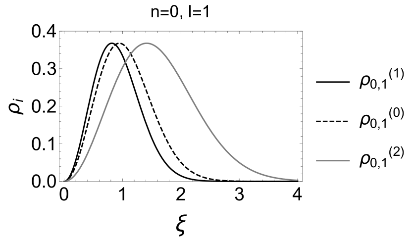
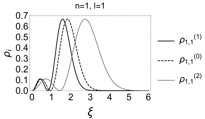
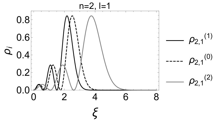
Figure 2: Probability distributions of the $l=1$ eigenstates (74) for (a) $n=0$ (top), (b) $n=1$ (center) and (c) $n=2$ (bottom) with $\omega=2\widetilde{\omega}=\frac{qB}{2mc}>0$ and $\xi=r/a$. The splitting implies the case $-\omega=2\widetilde{\omega}<0$ is obtained by exchanging $s_{1}$ and $s_{2}$ ($\rho_{1}\leftrightarrow\rho_{2}$), which means to reverse the direction of $\mathbf{B}$.

Analysis of the results

Now we analyze the energies and the eigenstates probability distributions. For fixing ideas we set $2|\widetilde{\omega}|=\omega$ and $\frac{m\omega a^{2}}{\hbar}=1$ so we have $\omega_{1}=\omega(1+\frac{1}{2}\textrm{sign}(\widetilde{\omega}))$, $\omega_{0}=\frac{\sqrt{5}}{2}\omega$, and $\omega_{2}=\omega(1-\frac{1}{2}\textrm{sign}(\widetilde{\omega}))$. If we define $\alpha_{i}=\frac{m\omega_{i}a^{2}}{\hbar}$ it follows that $\alpha_{1}=1+\frac{1}{2}\textrm{sign}(\widetilde{\omega})$, $\alpha_{0}=\sqrt{5}/2$ and $\alpha_{2}=1-\frac{1}{2}\textrm{sign}(\widetilde{\omega})$, where $\textrm{sign}(\gamma)$ denotes the sign function of $\gamma$ for all $\gamma\in\mathbf{R}$. Their corresponding probability distributions are obtained from the squared modulus of (46) and (66), expressed in the compact form by

$$\rho_{n,l}^{(i)}(\xi)=\left|\alpha_{i}\xi^{2}\right|^{|l|}e^{-\alpha_{i}\xi^{2}}L^{2|l|}_{n}\left(\alpha_{i}\xi^{2}\right),$$ (74)

with $i=0,1,2$, $\xi=r/a$ a dimensionless variable and $a$ a characteristic length (whose meaning will be clear later). The dependence in $\theta$ has disappeared due to the spherical symmetry of the problem. In order to study the interplay between the splitting and the energies, from (45) and (65) we can recast the energies for the splitting as

$$(\epsilon_{n,l}^{(i)})^{2}=$$

$$1-\frac{2\hbar(|l|\widetilde{\omega}+\omega)}{mc^{2}}\delta_{0i}+\frac{\hbar\omega_{i}}{mc^{2}}\left(4n+2|l|\left(1-s_{i}\right)+2(s_{i}+\delta_{0i})\right),$$ (75)

where $\epsilon_{n,l}^{i}$ are the energies adimensionalized by $mc^{2}$, $\delta_{0i}$ the Kronecker delta, $i=0,1,2$ and $s_{0}=0,s_{1}=-s_{2}=1$.

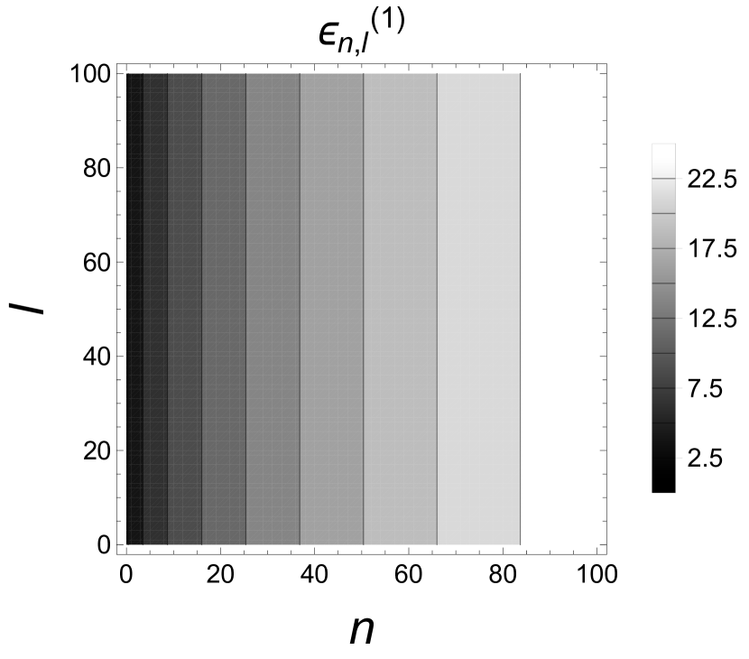
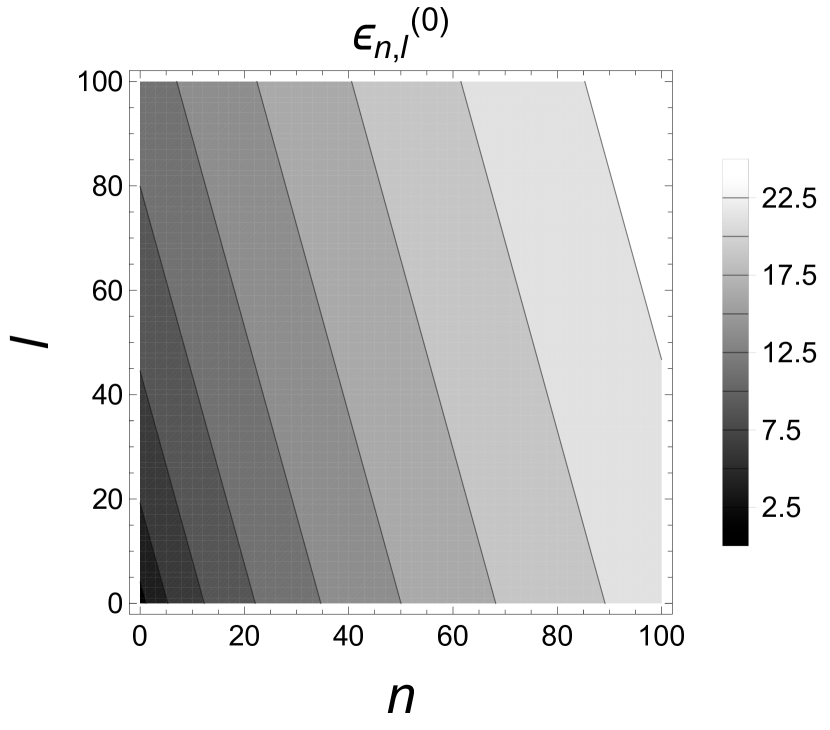
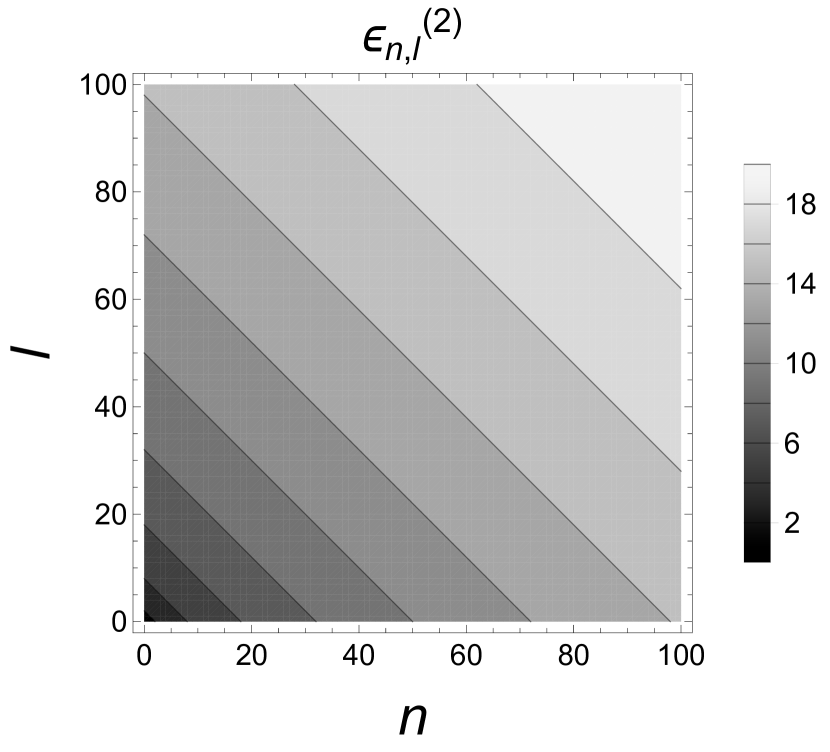
Figure 3: Contour plots of the splitting energy levels (76): (a) $s_{1}=1$ (top), (b) $s_{0}=0$ (center) and (c) $s_{2}=-1$ (bottom) for $\omega=2\widetilde{\omega}=\frac{qB}{2mc}>0$ within the range $0\leq n,l\leq 100$, . Due to the symmetry of (76) around $l=0$, i.e. $\epsilon_{n,l}^{(i)}=\epsilon_{n,-l}^{(i)}$, only the positive range of $l$ is shown. The lines indicate the degeneracy whose slopes are, from (Analysis of the results), $\infty$, $-\frac{2}{1-\frac{1}{\sqrt{5}}}$ and $-1$ for $s_{1}=1$, $s_{0}=0$, and $s_{2}=-1$.

For compatibilizing with $\frac{m\omega a^{2}}{\hbar}=1$ we set $\frac{\hbar\omega}{mc^{2}}=1$ so the characteristic length $a$ results to be the Compton wavelength $a=\frac{\hbar}{mc}$, which is a natural representation for mass on the quantum scale. The formula (75) turns out

$$(\epsilon_{n,l}^{(i)})^{2}=1$$

$$-(|l|\textrm{sign}(\widetilde{\omega})+2)\delta_{0i}+\alpha_{i}\left(4n+2|l|\left(1-s_{i}\right)+2(s_{i}+\delta_{0i})\right).$$ (76)

In Fig. 2 we show the probability distributions (74) of the $l=1$ eigenstates $\varphi_{i}$ with $i=0,1,2$ for $n=0,1,2$ and $\widetilde{\omega}>0$. We can see that the distributions of the spin projections $s_{1}=1$ and $s_{0}=0$ are close while the corresponding to $s_{2}=-1$ exhibits a different behavior, as a consequence of the splitting frequencies. In Fig. 3 we show the energies (76) of the eigenstates $\varphi_{i}$ for $0\leq n,l\leq 100$ and $\widetilde{\omega}>0$. The straight lines of Fig. 3 correspond to the degenerated states whose slopes are only depending on the sign of $\widetilde{\omega}$, that is, they are in function of the sign of $\mathbf{B}$. In fact, by letting $\varepsilon_{n,l}^{(i)}=k_{i}=\textrm{constant}$ in (75) the curves $l=l(n)$ of degeneracy in the range $l\geq 0$ have the slopes

$$-\frac{2}{1-\frac{\widetilde{\omega}}{\sqrt{\omega^{2}+\widetilde{\omega}^{2}}}}\quad, \quad\textrm{for}\quad s_{0}=0$$

$$-\frac{2}{1-s_{i}}\quad, \quad\textrm{for}\quad s_{1}=-s_{2}=1$$ (77)

where $\omega_{1,2}\neq 0$. From (75) some more features about the energies can be highlighted. For the component of projection $s_{1}=1$ the vibrational ($l=0$) and rotational ($l\neq 0$) states with quantum number $n$ have identical energy, so the magnetic field turns off the angular momentum and spin effects. It is also worth noting that in virtue of the splitting, the case $\widetilde{\omega}<0$ has the same eigenfunctions and energies but with the components flipped $\varphi_{1}\rightarrow\varphi_{2}$, while $\varphi_{0}$ remains invariant.

Thermodynamics of the vectorial sector

We illustrate the effect of the splitting in the statistical properties of the vectorial sector of the DKP oscillator since the scalar sector does not exhibit a cancellation of the oscillation. For accomplish this, we consider that the system is at equilibrium with a thermal bath of finite temperature $T$ in order to obtain the partition function of its canonical ensemble. Also, we consider only the states with positive energy due to those with negative energy are unlimited below, thus ensuring a stable ensemble [41]. Then, the partition function results

$$Z=\left(\sum_{n_{1},l_{1}}\exp\left(-\gamma y_{n_{1},l_{1}}\right)\right)\times\left(\sum_{n_{2},l_{2}}\exp\left(-\gamma y_{n_{2},l_{2}}\right)\right)$$ (78)

with $\gamma=\frac{mc^{2}}{k_{B}T}$ and

$$y_{n_{i},l_{i}}^{2}=1+\alpha_{i}\left(4n_{i}+2|l_{i}|\left(1-s_{i}\right)+2s_{i})\right)\quad,\quad i=1,2.$$ (79)

Here $k_{B}$ is the Boltzmann constant and we have employed again $\alpha_{i}=\frac{\hbar\omega_{i}}{mc^{2}}$ with $\omega_{i}=\omega+s_{i}\widetilde{\omega}$ for $i=1,2$. For facilitating the calculations we make $\frac{\hbar\omega}{mc^{2}}=1/2$ and then $\alpha_{i}=\frac{1}{2}(1+s_{i}\delta)$ with $\widetilde{\omega}=\delta\omega$. We also consider $\delta\in[0,\infty)$ to avoid negative expressions in the right hand of (79) and thus to simplify the counting of degeneracies. Since $y_{n_{1},l_{1}}^{2}=2(1+\delta)n_{1}+2+\delta$ and $y_{n_{2},l_{2}}^{2}=2(1-\delta)(n_{2}+|l_{2}|)+\delta$ we can calculate the sums of (78) separately by means of the general formula

$$\sum_{k}\Omega(E_{k})\exp\left(-\beta E_{k}\right),$$ (80)

where $\Omega(E_{k})$ indicates the degeneracy of the energy level $E_{k}$. For avoiding the infinite degeneracy of $y_{n_{1},l_{1}}$ in $l_{1}$ we assume that $\Omega(E_{n_{1},l_{1}})=\sum_{n_{1}=-l}^{n_{1}}=2n_{1}$, which physically means that only the states with $|l_{1}|\leq n_{1}$ contribute significatively to $E_{n_{1},l_{1}}$ and the rest of terms can be neglected. Then, we have

$$\sum_{n_{1},l_{1}}\exp\left(-\gamma y_{n_{1},l_{1}}\right) = \sum_{n=0}^{\infty}\sum_{l=-n}^{n}\exp\left(-\gamma\sqrt{2(1+\delta)n+2+\delta}\right)$$ (81)

$$= 2\sum_{n=0}^{\infty}n\exp\left(-\gamma\sqrt{2(1+\delta)n+2+\delta}\right).$$

For $y_{n_{2},l_{2}}$ we have a double degeneracy given by all the pairs $(n_{2},l_{2})$ such that $n_{2}+l_{2}=k\in\mathbf{N}_{0}$ with $n_{2},l_{2}=0,\ldots,k$. This implies that $\Omega(E_{n_{2},l_{2}})=2\sum^{k+1}1=2(k+1)$ for $\beta E_{n_{2},l_{2}}=k$. Then, we have

$$\sum_{n_{2},l_{2}}\exp\left(-\gamma y_{n_{2},l_{2}}\right)=$$

$$2\sum_{n=0}^{\infty}(n+1)\exp\left(-\gamma\sqrt{2(1-\delta)n+\delta}\right).$$ (82)

The sums (81) and (Thermodynamics of the vectorial sector) can be calculated with the help of the Euler-Maclaurin’s formula (employed in relativistic contexts for instance in [41, 42])

$$\sum_{n=0}^{\infty}f(n)=\frac{1}{2}f(0)+\int_{0}^{\infty}f(x)dx-\sum_{p=1}^{\infty}\frac{1}{(2p)!}B_{2p}f^{2p-1}(0),$$ (83)

with $B_{2p}$ the Bernoulli’s numbers and $f^{2p-1}(0)$ the derivatives of odd order of $f(x)$ at $x=0$. Now the crucial observation is that in the limit of high thermal excitations $\gamma=\frac{mc^{2}}{k_{b}T}\ll 1$ since the first and third terms of (83) only have powers of $\gamma$ and the integral has powers of $\gamma^{-1}$, then it is enough to consider only the integral , i.e.

$$Z\approx\left(2\int_{0}^{\infty}x\exp\left(-\gamma\sqrt{2(1+\delta)x+2+\delta}\right)dx\right)\times$$

$$\left(2\int_{0}^{\infty}(x+1)\exp\left(-\gamma\sqrt{2(1-\delta)x+\delta}\right)dx\right)\quad\textrm{for}\ \gamma\ll 1.$$ (84)

Using in (Thermodynamics of the vectorial sector) that for $a,b,\gamma\geq 0$

$$\int_{0}^{\infty}x\exp\left(-\gamma\sqrt{ax+b}\right)dx=\frac{4e^{-\gamma\sqrt{b}}\left(b\gamma^{2}+3\sqrt{b}\gamma+3\right)}{a^{2}\gamma^{4}}$$

$$\int_{0}^{\infty}(x+1)\exp\left(-\gamma\sqrt{ax+b}\right)dx=$$

$$\frac{2e^{-\gamma\sqrt{b}}\left(\sqrt{b}\gamma\left(a\gamma^{2}+6\right)+a\gamma^{2}+2b\gamma^{2}+6\right)}{a^{2}\gamma^{4}},$$ (85)

we obtain the partition function of the vectorial sector for $\gamma\ll 1$

$$Z(\gamma,\delta)=\left(\frac{2e^{-\gamma\sqrt{2+\delta}}\left((2+\delta)\gamma^{2}+3\sqrt{2+\delta}\gamma+3\right)}{(1+\delta)^{2}\gamma^{4}}\right)\times$$

$$\left(\frac{e^{-\gamma\sqrt{\delta}}\left(\sqrt{\delta}\gamma\left((1-\delta)\gamma^{2}+6\right)+(1-\delta)\gamma^{2}+2\delta\gamma^{2}+6\right)}{(1-\delta)^{2}\gamma^{4}}\right).$$ (86)

Thus, the partition function (Thermodynamics of the vectorial sector) results expressed in function of $\delta$ and $\gamma=\frac{mc^{2}}{k_{B}T}$, with the latter measuring the ratio between the rest mass and the thermal energy. It is worth noting that $Z(\gamma,\delta)\neq Z(\gamma,-\delta)$ due to the spectrum of $\varphi_{1}$ and $\varphi_{2}$ is not flipped when $\delta\rightarrow-\delta$. In the high temperature limit $T\rightarrow\infty$ we have $Z(\gamma,\delta)\approx\frac{6}{(1+\delta)^{2}\gamma^{4}}\frac{6}{(1-\delta)^{2}\gamma^{4}}$ and then the partition function results symmetric in $\delta$. On the other hand, the partition function (Thermodynamics of the vectorial sector) is real for $0\leq\delta\leq 1$ and when $\delta>1$ results complex, presenting divergences in all the interval $(1,\infty)$. In view of (Thermodynamics of the vectorial sector) we can see that the individual partition functions of $\varphi_{1}$ and $\varphi_{2}$ have the same structure $\propto 1/((1+s_{i}\delta)^{2}\gamma^{4})$, thus expressing that only the component $\varphi_{2}$ experiments a phase transition when $\delta\rightarrow 1$. This corresponds to the particle free case $\widetilde{\omega}=\omega$ with $\omega_{2}\rightarrow 0$, as pointed out previously. From the thermodynamic relations in function of the dimensionless variable $\gamma$ [41]

$$U = -mc^{2}\frac{\partial\ln Z}{\partial\gamma}\quad\textrm{(internal energy)}$$

$$F = -mc^{2}\frac{1}{\gamma}\ln Z\quad\textrm{(Helmholtz free energy)}$$

$$S = k_{B}\gamma^{2}\frac{\partial F}{\partial\gamma}\quad\textrm{(entropy)}$$

$$C = -k_{B}\gamma^{2}\frac{\partial U}{\partial\gamma}\quad\textrm{(specific heat)},$$ (87)

we derive the thermodynamics of the vectorial sector of the DKP oscillator. Substituting (Thermodynamics of the vectorial sector) in (Thermodynamics of the vectorial sector) we illustrate in Fig. 4 the internal energy, the entropy and the specific heat.

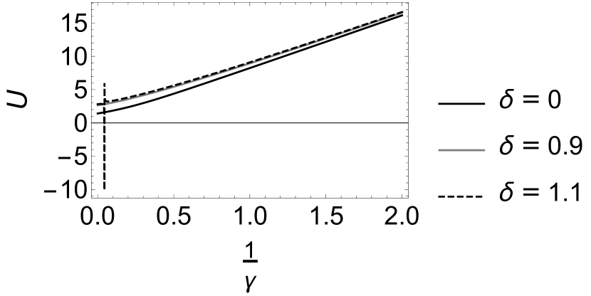
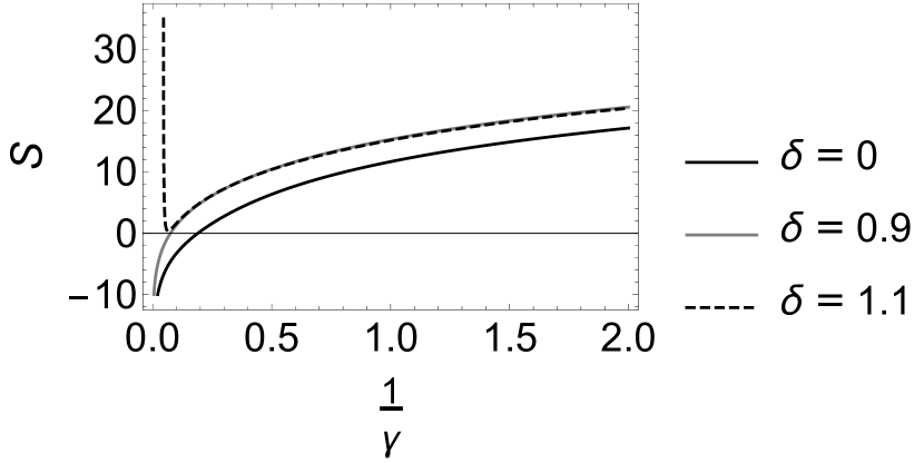
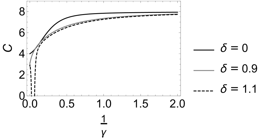
Figure 4: (a) Internal energy (top), (b) entropy (center) and (d) specific heat (bottom) of the vectorial sector of the two-dimensional DKP oscillator in an external magnetic field $\mathbf{B}=B\hat{z}$ in function of the real parameter $\delta\in[0,\infty)$, with $\delta=\frac{qB}{mc\omega}$ and $\omega=\frac{mc^{2}}{2\hbar}$ the oscillator frequency. The discontinuity of the dashed curves indicate the phase transition that occurs around $\delta=1$ due to the cancellation of the oscillation of the 2-component.

We can see that the thermodynamic potentials rapidly converge to their asymptotical behaviors when $1/\gamma\rightarrow\infty(T\rightarrow\infty)$, in virtue of that the thermal excitations erase the particularities of the vectorial sector spectrum as soon as the only relevant term in the total partition function (Thermodynamics of the vectorial sector) is proportional to $T^{8}$. From (Thermodynamics of the vectorial sector) the asymptotical expressions of (Thermodynamics of the vectorial sector), that also show the additivity property in the vectorial sector, are given by

$$U\approx 8k_{B}T=4k_{B}T+4k_{B}T=U_{1}+U_{2}$$

$$F\approx-8k_{B}T\ln\left(\frac{k_{B}T}{mc^{2}(1-\delta^{2})^{1/4}}\right)=$$

$$-4k_{B}T\ln\left(\frac{k_{B}T}{mc^{2}(1+\delta)^{1/4}}\right)-4k_{B}T\ln\left(\frac{k_{B}T}{mc^{2}(1-\delta)^{1/4}}\right)$$

$$=F_{1}+F_{2}$$

$$S\approx 8k_{B}\left(\ln\left(\frac{k_{B}T}{mc^{2}(1-\delta^{2})^{1/4}}\right)+1\right)=$$

$$4k_{B}\left(\ln\left(\frac{k_{B}T}{mc^{2}(1+\delta)^{1/4}}\right)+1\right)+4k_{B}\left(\ln\left(\frac{k_{B}T}{mc^{2}(1-\delta)^{1/4}}\right)+1\right)$$

$$C\approx 8k_{B}=4k_{B}+4k_{B}=C_{1}+C_{2}.$$ (88)

Conclusions

We have revisited the $(2+1)$-dimensional DKP oscillator in an external magnetic field from scalar $4\times 4$ and vectorial $6\times 6$ representations, which allow to study several cases of the literature as well as calculating their energies and eigenfunctions, in a unified way. The energies and eigenfunctions for the scalar DKPO in a uniform magnetic field are shown in the equations (45)-(46), respectively, where the angular frequency $\omega$ is replaced by $\omega_{0}=\sqrt{\omega^{2}+\widetilde{\omega}^{2}}$ being $\widetilde{\omega}=\frac{qB}{mc}$ the field angular frequency. The vector DKPO interacting with a magnetic field presents a splitting $\omega\rightarrow(\omega_{1},\omega_{0},\omega_{2})$ in the frequency of the oscillation (Fig. 1), that corresponds to the spin projections $s_{i}=+1,0,-1$ of the vector DKP field. The energies and the eigenfunctions of this oscillator are presented in (45), (46), (65), (66) and some of them illustrated in Figs. 2, 3, where the slopes of the degeneracies (Analysis of the results) are in function of $\omega$, $\widetilde{\omega}$ and $s_{i}$. Some special cases have been studied with two critical ones when $\widetilde{\omega}=\pm\omega\rightarrow\mathbf{B}=\pm\frac{2mc\omega}{q}\hat{z}$. In these cases the component $\varphi_{1}$ or $\varphi_{2}$ stops oscillating, where the phase transition $\widetilde{\omega}\rightarrow\omega$ has been characterized by means of the canonical ensemble of the vectorial sector. The thermodynamic potentials exhibit a rapid convergence to their asymptotical expressions due to the thermal excitations (Fig. 4), thus resulting the partition function (Thermodynamics of the vectorial sector) $\propto T^{8}$ and the individual ones $\propto T^{4}$, with the divergences associated to the critical values of the magnetic field.

References

• [1] R. J. Duffin, Phys. Rev. 54, 1114 (1938).
• [2] N. Kemmer, Proc. R. Soc. A 173, 91 (1939).
• [3] G. Petiau, Acad. R. Belg. Cl. Sci. MΓ©m. Collect. 8, 16 No 2 (1936).
• [4] R. A. Krajcik and M. M. Nieto, Am. J. Phys. 45, 818 (1977).
• [5] E. M. Corson, in Introduction to Tensors, Spinors, and Relativistic Wave-Equations, (Blackie and Sons, London, 1953).
• [6] M. Montigny and E. S. Santos, J. Math. Phys. 60, 082302 (2019).
• [7] H. Umezawa, in Quantum Field Theory, (North-Holland, Amsterdam, 1956).
• [8] J. T. Lunardi, B. M. Pimentel, R. G. Teixeira, and J. S. Valverde, Phys. Lett. A 268, 165 (2000).
• [9] R. F. Guertin and T. L. Wilson, Phys. Rev. D 15, 1528 (1977).
• [10] L. Kurth Kerr, B. C. Clark, S. Hama, L. Ray, and G. W. Hoffmann, Prog. Theor. Phys. 103, 321 (2000).
• [11] V. Gribov, Eur. Phys. J. C 10, 71 (1999); 10, 91 (1999).
• [12] V. Ya. Fainberg and B. M. Pimentel, Theor. Math. Phys. 124, 1234 (2000).
• [13] J. T. Lunardi, L. A. Manzoni, B. M. Pimentel, and J. S. Valverde, Int. J. Mod. Phys. A 17, 205 (2002).
• [14] L. M. Abreu, E. S. Santos, and J. D. M. Vianna. J. Phys. A: Math. Theor. 43, 495402 (2010).
• [15] R. Casana, V. Ya. Fainberg, B. M. Pimentel and J. S. Valverde, Phys. Lett. A 316, 33 (2003).
• [16] L. M. Abreu, A. L. Gadelha, B. M. Pimentel and E. S. Santos, Physica A 419, 612 (2015).
• [17] H. Belich, E. Passos, M. D. Montigny, and E. S. Santos, Int. J. Mod. Phys. A 33, 1850165 (2018).
• [18] R. Casana, C. A. M. de Melo, and B. M. Pimentel, Class. Quantum Grav. 24, 723 (2007).
• [19] A. Boumali. Can. J. Phys. 85, 1417 (2007).
• [20] J. A. Swansson et al., J. Phys. A: Math. Gen. 34, 1051 (2001).
• [21] M. Montigny, F. C. Khanna, A. E. Santana, E. S. Santos, and J. D. M. Vianna, J. Phys. A: Math. Gen. 33, L273 (2000).
• [22] M. Montigny, F. C. Khanna, A. E. Santana, E. S. Santos and J. D. M. Vianna, J. Phys. A: Math. Gen. 34, 8901 (2001).
• [23] E. S. Santos and L. M. Abreu, J. Phys. A: Math. Theor. 41, 075407 (2008).
• [24] Y. Nedjadi and R. C. Barret, J. Phys. A: Math. Gen. 27, 4301 (1994).
• [25] A. Boumali. J. Phys. A: Math. Gen. 42, 235301 (2009).
• [26] M. C. B. Fernandes and J. D. M. Vianna. Braz. J. Phys. 29, 487 (1998).
• [27] B. Boutabia-ChΓ©raitia and T. Boudjedaa. Phys. Lett. A 338, 97 (2005).
• [28] P. Ghose, M. K. Samal and A. Datta, Phys. Lett. A 315, 23 (2003).
• [29] J. T. Lunardi, B. M. Pimentel and R. G. Teixeira. Gen. Relativ. Gravit. 34, 491 (2002).
• [30] H. Hassanabadi, B. H. Yazarloo, S. Zarrinkamar, and A. A. Rajabi, Phys. Rev. C 84, 064003 (2011).
• [31] B. Mirza, R. Narimani and S. Zare, Commun. Theor. Phys. 55, 405 (2011).
• [32] L. B. Castro and A. S. Castro, Phys. Lett. A 375, 2596 (2011).
• [33] H. Hassanabadi, Z. Molaee and S. Zarrinkamar, Eur. Phys. J. C 72, 2217 (2012).
• [34] A. Boumali, L. Chatouani and H. Hassanabadi, Can. J. Phys. 91, 1 (2013).
• [35] L. B. Castro and A. S. Castro, Phys. Rev. A 90, 022101 (2014).
• [36] S-r. Wu, Z-w. Long, C-y. Long, B-q. Wang and Y. Liu, Eur. Phys. J. Plus 132 186 (2017).
• [37] Y. Chargui, Phys. Lett. A 382, 949 (2018).
• [38] M. Falek, M. Merad and M. Moumni J. Math. Phys. 60, 013505 (2019).
• [39] B. P. Mandal and S. Verma, Phys. Lett. A 374, 1021 (2010).
• [40] V. Tyagi, S. K. Rai and B. P. Mandal, EPL 128, 30004 (2019).
• [41] M. H. Pacheco, R. V. Maluf, C. A. S. Almeida and R. R. Landim, EPL 108, 10005 (2014).
• [42] K. Nouicer, J. Phys. A: Math. Gen. 39, 5125-5134 (2006).