Graph Homomorphism Convolution
Abstract
In this paper, we study the graph classification problem from the graph homomorphism perspective. We consider the homomorphisms from to , where is a graph of interest (e.g. molecules or social networks) and belongs to some family of graphs (e.g. paths or non-isomorphic trees). We show that graph homomorphism numbers provide a natural invariant (isomorphism invariant and -invariant) embedding maps which can be used for graph classification. Viewing the expressive power of a graph classifier by the -indistinguishable concept, we prove the universality property of graph homomorphism vectors in approximating -invariant functions. In practice, by choosing whose elements have bounded tree-width, we show that the homomorphism method is efficient compared with other methods.
1 Introduction
1.1 Background
In many fields of science, objects of interest often exhibit irregular structures. For example, in biology or chemistry, molecules and protein interactions are often modeled as graphs (Milo et al., 2002; Benson et al., 2016). In multi-physics numerical analyses, methods such as the finite element methods discretize the sample under study by 2D/3D-meshes (Mezentsev, 2004; Fey et al., 2018). In social studies, interactions between people are presented as a social network (Barabási et al., 2016). Understanding these irregular non-Euclidean structures have yielded valuable scientific and engineering insights. With recent successful developments of machine learning on regular Euclidean data such as images, a natural extension challenge arises: How do we learn non-Euclidean data such as graphs or meshes?
Geometric (deep) learning (Bronstein et al., 2017) is an important extension of machine learning as it generalizes learning methods from Euclidean data to non-Euclidean data. This branch of machine learning not only deals with learning irregular data but also provides a proper means to combine meta-data with their underlying structure. Therefore, geometric learning methods have enabled the application of machine learning to real-world problems: From categorizing complex social interactions to generating new chemical molecules. Among these methods, graph-learning models for the classification task have been the most important subject of study.
Let be the space of features (e.g., for some positive integer ), be the space of outcomes (e.g., ), and be a graph with a vertex set and edge set . The graph classification problem is stated follow111This setting also includes the regression problem..
Problem 1 (Graph Classification Problem).
We are given a set of tuples of graphs , vertex features , and outcomes . The task is to learn a hypothesis such that . 222 can be a machine learning model with a given training set.
Problem 1 has been studied both theoretically and empirically. Theoretical graph classification models often discuss the universality properties of some targeted function class. While we can identify the function classes which these theoretical models can approximate, practical implementations pose many challenges. For instance, the tensorized model proposed by (Keriven & Peyré, 2019) is universal in the space of continuous functions on bounded size graphs, but it is impractical to implement such a model. On the other hand, little is known about the class of functions which can be estimated by some practical state-of-the-art models. To address these disadvantages of both theoretical models and practical models, we need a practical graph classification model whose approximation capability can be parameterized. Such a model is not only effective in practice, as we can introduce inductive bias to the design by the aforementioned parameterization, but also useful in theory as a framework to study the graph classification problem.
In machine learning, a model often introduces a set of assumptions, which is known as inductive bias. These assumptions help narrow down the hypothesis space while maintaining the validity of the learning model subject to the nature of the data. For example, a natural inductive bias for graph classification problems is the invariant to the permutation property (Maron et al., 2018; Sannai et al., 2019). We are often interested in a hypothesis that is invariant to isomorphism, i.e., for two isomorphic graphs and the hypothesis should produce the same outcome, . Therefore, it is reasonable to restrict our attention to only invariant hypotheses. More specifically, we focus on invariant embedding maps because we can construct an invariant hypothesis by combining these mappings with any machine learning model designed for vector data. Consider the following research question:
Question 2.
How to design an efficient and invariant embedding map for the graph classification problem?
1.2 Homomorphism Numbers as a Classifier
A common approach to Problem 1 is to design an embedding333Not to be confused with “vertex embedding”. , which maps graphs to vectors, where is the dimensionality of the representation. Such an embedding can be used to represent a hypothesis for graphs as by some hypothesis for vectors. Because the learning problem on vectors is a well-studied problem, we can focus on designing and understanding graph embedding.
We found that using homomorphism numbers as an invariant embedding is not only theoretically valid but also extremely efficient in practice. In a nutshell, the embedding for a graph is given by selecting pattern graphs to form a fixed set , then computing the homomorphism numbers from each to . The classification capability of the homomorphism embedding is parameterized by . We develop rigorous analyses for this idea in Section 2 (without vertex features) and Section 3 (with vertex features).
Our contribution is summarized as follows:
-
•
Introduce and analyze the usage of weighted graph homomorphism numbers with a general choice of . The choice of is a novel way to parameterize the capability of graph learning models compared to choosing the tensorization order in other related work.
-
•
Prove the universality of the homomorphism vector in approximating -indistinguishable functions. Our main proof technique is to check the condition of the Stone-Weierstrass theorem.
-
•
Empirically demonstrate our theoretical findings with synthetic and benchmark datasets. Notably, we show that our methods perform well in graph isomorphism test compared to other machine learning models.
In this paper, we focus on simple undirected graphs without edge weights for simplicity. The extension of all our results to directed and/or weighted graphs is left as future work.
1.3 Related Works
There are two main approaches to construct an embedding: graph kernels and graph neural networks. In the following paragraphs, we introduce some of the most popular methods which directly related to our work. For a more comprehensive view of the literature, we refer to surveys on graph neural networks (Wu et al., 2019) and graph kernels (Gärtner, 2003; Kriege et al., 2019).
1.3.1 Graph Kernels
The kernel method first defines a kernel function on the space, which implicitly defines an embedding such that the inner product of the embedding vectors gives a kernel function. Graph kernels implement by counting methods or graph distances (often exchangeable measures). Therefore, they are isomorphism-invariant by definition.
The graph kernel method is the most popular approach to study graph embedding maps. Since designing a kernel which uniquely represents graphs up to isomorphisms is as hard as solving graph isomorphism (Gärtner et al., 2003), many previous studies on graph kernels have focused on proposing a solution to the trade-off between computational efficiency and representability. A natural idea is to compute subgraph frequencies (Gärtner et al., 2003) to use as graph embeddings. However, counting subgraphs is a #W[1]-hard problem (Flum & Grohe, 2006) and even counting induced subgraphs is an NP-hard problem (more precisely it is an #A[1]-hard problem (Flum & Grohe, 2006)). Therefore, methods like the tree kernel (Collins & Duffy, 2002; Mahé & Vert, 2009) or the random walk kernel (Gärtner et al., 2003; Borgwardt et al., 2005) restrict the subgraph family to be some computationally efficient graphs. Regarding graph homomorphism, Gärtner et al. and also Mahé & Vert studied a relaxation which is similar to homomorphism counting (walks and trees). Especially, Mahé & Vert showed that the tree kernel is efficient for molecule applications. However, their studies limit to tree kernels and it is not known to what extend these kernels can represent graphs.
More recently, the graphlet kernel (Shervashidze et al., 2009; Pržulj et al., 2004) and the Weisfeiler-Lehman kernel (Shervashidze et al., 2011; Kriege et al., 2016) set the state-of-the-art for benchmark datasets (Kersting et al., 2016). Other similar kernels with novel modifications to the distance function, such as Wasserstein distance, are also proposed (Togninalli et al., 2019). While these kernels are effective for benchmark datasets, some are known to be not universal (Xu et al., 2019; Keriven & Peyré, 2019) and it is difficult to address their expressive power to represent graphs.
1.3.2 Graph Neural Networks
Graph Neural Networks refers to a new class of graph classification models in which the embedding map is implemented by a neural network. In general, the mapping follows an aggregation-readout scheme (Hamilton et al., 2017; Gilmer et al., 2017; Xu et al., 2019; Du et al., 2019) where vertex features are aggregated from their neighbors and then read-out to obtain the graph embedding. Empirically, especially on social network datasets, these neural networks have shown better accuracy and inference time than graph kernels. However, there exist some challenging cases where these practical neural networks fail, such as Circular Skip Links synthetic data (Murphy et al., 2019) or bipartite classification (Section 4).
Theoretical analysis of graph neural networks is an active topic of study. The capability of a graph neural network has been recently linked to the Weisfeiler-Lehman isomorphism test (Morris et al., 2019; Xu et al., 2019). Since Morris et al. and Xu et al. proved that the aggregation-readout scheme is bounded by the one-dimensional Weisfeiler-Lehman test, much work has been done to quantify and improve the capability of graph neural networks via the tensorization order. Another important aspect of graph neural networks is their ability to approximate graph isomorphism equivariant or invariant functions (Maron et al., 2018, 2019; Keriven & Peyré, 2019). Interestingly, Chen et al. showed that isomorphism testing and function approximation are equivalent.
The advantage of tensorized graph neural networks lies in their expressive power. However, the disadvantage is that the tensorization order makes it difficult to have an intuitive view of the functions which need to be approximated. Furthermore, the empirical performance of these models might heavily depends on initialization (Chen et al., 2019).
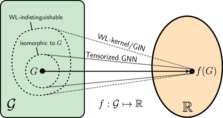
Figure 1 visualizes the interaction between function approximation and isomorphism testing. An ideal graph neural network maps only and graphs isomorphic to it to . On the other hand, efficient implementation of can only maps some -indistinguishable of to . This paper shows that graph homomorphism vectors with some polynomials universally approximate -invariant functions.
2 Graphs without Features
We first establish our theoretical framework for graphs without vertex features. Social networks are often feature-less graphs, in which only structural information (e.g. hyperlinks, friendships, etc.) is captured. The main result of this section is to show that using homomorphism numbers with some polynomial not only yields a universally invariant approximator but that we can also select the pattern set for some targeted applications.
2.1 Definition
An (undirected) graph is simple if it has neither self-loops nor parallel edges. We denote by the set of all simple graphs.
Let be a graph. For a finite set and a bijection , we denote by the graph defined by and . Two graphs and are isomorphic if for some bijection .
2.2 Homomorphism Numbers
Here, we introduce the homomorphism number. This is a well-studied concept in graph theory (Hell & Nesetril, 2004; Lovász, 2012) and plays a key role in our framework.
Let and be undirected graphs. A homomorphism from to is a function that preserves the existence of edges, i.e., implies . We denote by the set of all homomorphisms from to . The homomorphism number is the cardinality of the homomorphisms, i.e., . We also consider the homomorphism density . This is a normalized version of the homomorphism number:
| (1) | ||||
| (2) |
where is the Iverson braket. Eq. (2) can be seen as the probability that randomly sampled vertices of preserve the edges of . Intuitively, a homomorphism number aggregates local connectivity information of using a pattern graph .
Example 3.
Let be a single vertex, we have and .
Example 4.
Let be the star graph of size . Then, , where is the degree of vertex .
Example 5.
We have: , where is a length cycle and is the adjacency matrix of .
It is trivial to see that the homomorphism number is invariant under isomorphism. Surprisingly, the converse holds as homomorphism numbers identify the isomorphism class of a graph. Formally, we have the following theorem.
Theorem 6 ((Lovász, 1967)).
Two graphs and are isomorphic if and only if for all simple graphs . In addition, if then we only have to examine with .
2.3 Homomorphism Numbers as Embeddings
The isomorphism invariance of the homomorphism numbers motivates us to use them as the embedding vectors for a graph. Since examining all graphs will be impractical (i.e. ), we select a subset as a parameter for the graph embedding. We obtain the embedding vector of a graph by stacking the the homomorphism numbers from . When , this is known as the Lovász vector.
We focus on two criterion: Expressive capability and computational efficiency. Similar to the kernel representability and efficiency trade-off, a more expressive homomorphism embedding map is usually less efficient and vice versa.
Graphs and are defined to be -indistinguishable if for all (Böker et al., 2019). Theorem 6 implies that the -indistinguishability generalizes graph isomorphism. For several classes , the interpretation of -indistinguishability is studied; the results are summarized in Table 1. The most interesting result is the case when has treewidth444Smaller treewidth implies the graph is more “tree-like”. at most where the -indistinguishability coincides with the -dimensional Weisfeiler–Lehman isomorphism test (Dell et al., 2018).
| -indistinguishable | |
|---|---|
| single vertex | graphs have the same number of vertices (Example 3) |
| single edge | graphs have the same number of edges (Example 3) |
| stars | graphs have the same degree sequence (Example 4) |
| cycles | adjacency matrices have the same eigenvalues (Example 5) |
| treewidth up to | graphs cannot be distinguished by the -dimensional Weisfeiler-Lehman test (Dell et al., 2018) |
| all simple graphs | isomorphic graphs (Lovász, 1967) |
A function is -invariant if for all -indistinguishable and ; therefore, if we use the -homomorphism as an embedding, we can only represent -invariant functions. In practice, should be chosen as small as possible such that the target hypothesis can be assumed to be -invariant. In the next section, we show that any continuous -invariant function is arbitrary accurately approximated by a function of the -homomorphism embedding (Theorem 7 and 8).
2.4 Expressive Power: Universality Theorem
By characterizing the class of functions that is represented by , we obtain the following results.
Theorem 7.
Let be an -invariant function. For any positive integer , there exists a degree polynomial of s.t. with .
Theorem 8.
Let be a continuous -invariant function. There exists a degree polynomial of () such that .
Proof of Theorem 7.
Since , the graph space contains a finite number of points; therefore, under the discrete topology, the space is compact Hausdorff.555In this topology, any function is continuous. Let be a set of points (e.g., graphs). A set of functions separates if for any two different points , there exists a function such that . By this separability and the Stone–Weierstrass theorem (Theorem 9), we conclude the proof. ∎
Theorem 7 is the universal approximation theorem for bounded size graphs. This holds without any assumption of the target function . It is worth mentioning that the invariant/equivariant universality results of tensorized graph neural networks on this bounded size setting were proven by (Keriven & Peyré, 2019); the unbounded case remains an open problem. Theorem 8 is the universal approximation for all graphs (unbounded). This is an improvement to the previous works. However, our theorem only holds for continuous functions, where the topology of the space has to satisfy the conditions of the Stone-Weierstrass theorem.
Theorem 9 (Stone–Weierstrass Theorem (Hart et al., 2003)).
Let be a compact Hausdorff space and be the set of continuous functions from to . If a subset separates then the set of polynomials of is dense in w.r.t. the topology of uniform convergence.
In the unbounded graph case (Theorem 8), the input space contains infinitely many graphs; therefore, it is not compact under the discrete topology. Hence, we cannot directly apply the Stone–Weierstrass theorem as in the bounded case. To obtain a stronger result, we have to complete the set of all graphs, and prove the completed space is compact Hausdorff. Since it is non-trivial to work directly with discrete graphs, we find that the graphon theory (Lovász, 2012) fits our purpose.
Graphon
A sequence of graphs is a convergence if the homomorphism density, , is a convergence for all simple graph . A limit of a convergence is called a graphon, and the space obtained by adding the limits of the convergences is called the graphon space, which is denoted by . See (Lovász, 2012) for the detail of this construction. The following theorem is one of the most important results in graphon theory.
Theorem 10 (Compactness Theorem (Lovász, 2012; Lovász & Szegedy, 2006)).
The graphon space with the cut distance is compact Hausdorff.
Now we can prove the graphon version of Theorem 8.
Theorem 11.
Any continuous -invariant function is arbitrary accurately approximated by a polynomial of .
Proof.
The -indistinguishability forms a closed equivalence relation on , where the homomorphism density is used instead of the homomorphism number. Let be the quotient space of this equivalence relation, which is compact Hausdorff in the quotient topology.
By the definition of the quotient topology, any continuous -invariant function is identified as a continuous function on . Also, by the definition, the set of -homomorphisms separates the quotient space. Therefore, the conditions of the Stone–Weierstrass theorem (Theorem 9) are fulfilled. ∎
2.5 Computational Complexity: Bounded Treewidth
Computing homomorphism numbers is, in general, an #P-hard problem (Díaz et al., 2002). However, if the pattern graph has bounded treewidth, homomorphism numbers can be computed in polynomial time.
A tree-decomposition (Robertson & Seymour, 1986) of a graph is a tree with mapping such that (1) , (2) for any there exists such that , and (3) for any the set is connected in . The treewidth (abbreviated as “tw”) of is the minimum of for all tree-decomposition of .
Theorem 12 ((Díaz et al., 2002)).
For any graphs and , the homomorphism number is computable in time.
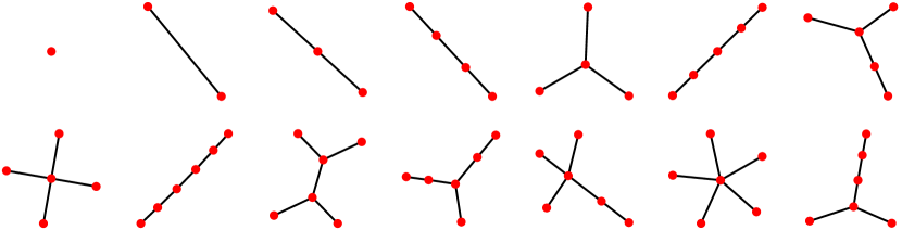
The most useful case will be when is the set of trees of size at most . The number of trees of size is a known integer sequence666https://oeis.org/A000055. There are 106 non-isomorphic trees of size , which is computationally tractable in practice. Also, in this case, the algorithm for computing is easily implemented by dynamic programming with recursion as in Algorithm 1. This algorithm runs in time. For the non-featured case, we sets . The simplicity of Algorithm 1 comes from the fact that if is a tree then we only need to keep track of a vertex’s immediate ancestor when we process that vertex by the visited argument in the function recursion.
3 Graphs with Features
Biological/chemical datasets are often modeled as graphs with vertex features (attributed graphs). In this section, we develop results for graphs with features.
3.1 Definition
A vertex-featured graph is a pair of a graph and a function , where .
Let be a vertex-featured graph. For a finite set and a bijection , we denote by the feature vector on such that . Two vertex-featured graphs and are isomorphic if and for some .
3.2 Weighted Homomorphism Numbers
We first consider the case that the features are non-negative real numbers. Let denote the feature of vertex , weighted homomorphism number is defined as follow:
| (3) |
and weighted homomorphism density is defined by . This definition coincides with the homomorphism number and density if for all .
The weighted version of the Lovász theorem holds as follows. We say that two vertices are twins if the neighborhood of and are the same. The twin-reduction is a procedure that iteratively selects twins and , contract them to create new vertex , and assign as a new weight. Note that the result of the process is independent of the order of contractions.
Theorem 13 ((Freedman et al., 2007), (Cai & Govorov, 2019)).
Two graphs and are isomorphic after the twin-reduction and removing vertices of weight zero if and only if for all simple graph .
Now we can prove a generalization of the Lovaász theorem.
Theorem 14.
Two graphs and are isomorphic if and only if for all simple graph and some continuous function .
Proof.
It is trivial to see that if and are isomorphic then they produce the same homomorphism numbers. Thus, we only have to prove the only-if part.
Suppose that the graphs are non-isomorphic. By setting , we have the same setting as the feature-less case; hence, by Theorem 6, we can detect the isomorphism classes of the underlying graphs.
Assuming and are isomorphic, we arrange the vertices of in the increasing order of the features (compared with the lexicographical order). Then, we arrange the vertices of lexicographically smallest while the corresponding subgraphs induced by some first vertices are isomorphic. Let us choose the first vertex whose feature is different to the feature of the corresponding vertex in . Then, we define
where stands for the lexicographical order. Then, we have as follows. Suppose that the equality holds. Then, by Theorem 13, the subgraphs induced by vertices whose features are lexicographicallly smaller than or equal to are isomorphic. However, this contradicts the minimality of the ordering of . Finally, by taking a continuous approximation of , we obtain the theorem. ∎
3.3 -Homomorphism Number
Let be a vertex-featured graph. For a simple graph and a function , -convolution is given by
| (4) |
The -convolution first transform the vertex features into real values by the encoding function . Then this aggregates the values by the pattern graph . The aggregation part has some similarity with the convolution in CNNs. Thus, we call this operation “convolution.”
Example 15.
Let be a singleton graph and be the -th component of the argument. Then,
| (5) |
Example 16.
Let be a graph of one edge and be the -th component of the argument. Then,
| (6) |
Algorithm 1 implements this idea when is the identity function. We see that the -convolution is invariant under graph isomorphism in the following result.
Theorem 17.
For a simple graph , a function , a vertex-featured graph , and a permutation on , we have
| (7) |
Proof.
Therefore, we have:
From the definition, we have . ∎
Theorem 17 indicates that for any and , the -convolution can be used as a feature map for graph classification problems. To obtain a more powerful embedding, we can stack multiple -convolutions. Let be a (possibly infinite) set of finite simple graphs and be a (possibly infinite) set of functions. Then -convolution, , is a (possibly infinite) vector:
| (8) |
By Theorem 17, for any and , the -convolution is invariant under the isomorphism. Hence, we propose to use -convolution as a embedding of graphs.
3.4 -Homomorphism Number as Embedding
Let be a set of continuous functions. As same as the featureless case, we propose to use the -homomorphism numbers as an embedding. We say that two featured graphs and are -indistinguishable if for all and . A function is -invariant if for all -indistinguishable and .
3.5 Universality Theorem
The challenge in proving the universality theorem for the featured setting is similar to the featureless case, which is the difficulty of the topological space. We consider the quotient space of graphs with respect to -indistinguishability. Our goal is to prove this space is completed to a compact Hausdorff space.
With a slight abuse of notation, consider a function that maps a vertex featured graph to a -dimensional vector where each coordinate is an equivalence class of -indistinguishable graphs. This space has a bijection to the quotient space by -indistinguishability. Each coordinate of the -dimensional space is completed to a compact Hausdorff space (Borgs et al., 2008). Therefore, by the Tychonoff product theorem (Hart et al., 2003), the -dimensional space is compact. The bijection between the quotient space shows the quotient space is completed by a compact Hausdorff space. We denote this space by . Under this space, we have the following result.
Theorem 18.
Any continuous -invariant function is arbitrary accurately approximated by a polynomial of .
Proof.
The space is compact by construction. The separability follows from the definition of -invariant. Therefore, by the Stone–Weierstrass theorem, we complete the proof. ∎
The strength of an embedding is characterized by the separability.
Lemma 19.
Let be the set of all simple graphs and be the set of all continuous functions from to . Then, is injective.
Proof.
Let and be two non-isomorphic vertex-featured graphs. We distinguish these graphs by the homomorphism convolution.
If and are non-isomorphic, by (Lovász, 1967), where is the function that takes one for any argument.
Now we consider the case that . Let be the set of vertices of . Without loss of generality, we assume where is the lexicographical order. Now we find a permutation such that and are lexicographically smallest. Let be the smallest index such that . By the definition, . We choose by
| (9) |
Then, there exists such that because the graphs induced by and are non-isomorphic because of the choice of .
Now we approximate by a continuous function . Because -convolution is continuous in the vertex weights (i.e., ), by choosing sufficiently close to , we get . ∎
We say that a sequence () of featured graphs is an -convergent if for each and the sequence () is a convergent in . A function is -continuous if for any -convergent (), the limit of the function exists and its only depends on the limits of the homomorphism convolutions for all and .
Now we prove the universality theorem. Let be a dense subset of the set of continuous functions, e.g., the set of polynomials or the set of functions represented by a deep neural network. We define by
| (10) |
where the argument of the function is restricted to . This is the set of functions obtained by combining universal approximators in and the homomorphism convolutions for some and . Let be a set of graphs, and let be the set of -continuous functions defined on . Then, we obtain the following theorem.
Theorem 20 (Universal Approximation Theorem).
Let be a compact set of graphs whose number of vertices are bounded by a constant. Then, is dense in .
Proof.
Because the number of vertices are bounded, the space of converging sequences is identified as . Therefore, this space is compact Hausdorff. The separability is proved in Lemma 19. Hence, we can use the Stone–Weierstrass theorem to conclude this result. ∎
3.6 The Choice of and
In an application, we have to choose and appropriately. The criteria of choosing them will be the same as with non-featured case: Trade-off between representability and efficiency. Representability requires that -convolutions can separate the graphs in which we are interested in. Efficiency requires that -convolutions must be efficiently computable. This trivially limits both and as finite sets.
The choice of will depend on the property of the vertex features. We will include the constant function if the topology of the graph is important. We will also include the -th component of the arguments. If we know some interaction between the features is important, we can also include the cross terms.
The choice of relates with the topology of the graphs of interest. If where is the constant function, the homomorphism convolution coincides with the homomorphism number (Table 1).
Here, we focus on the efficiency. In general, computing is #P-hard. However, it is computable in polynomial time if has a bounded tree The treewidth of a graph , denoted by , is a graph parameter that measures the tree-likeness of the graph. The following result holds.
Theorem 21.
is computable in time, is the treewidth of .
4 Experimental results
| Methods | CSL | BIPARTITE | PAULUS25 |
|---|---|---|---|
| Practical models | |||
| GIN | 10.00 0.00 | 55.75 7.91 | 7.14 0.00 |
| GNTK | 10.00 0.00 | 58.03 6.84 | 7.14 0.00 |
| Theory models | |||
| Ring-GNN | 1080 15.7 | 55.72 6.95 | 7.15 0.00 |
| GHC-Tree | 10.00 0.00 | 52.68 7.15 | 7.14 0.00 |
| GHC-Cycle | 100.0 0.00 | 100.0 0.00 | 7.14 0.00 |
| Methods | MUTAG | IMDB-BIN | IMDB-MUL |
|---|---|---|---|
| Practical models | |||
| GNTK | 89.46 7.03 | 75.61 3.98 | 51.91 3.56 |
| GIN | 89.40 5.60 | 70.70 1.10 | 43.20 2.00 |
| PATCHY-SAN | 89.92 4.50 | 71.00 2.20 | 45.20 2.80 |
| WL kernel | 90.40 5.70 | 73.80 3.90 | 50.90 3.80 |
| Theory models | |||
| Ring-GNN | 78.07 5.61 | 73.00 5.40 | 48.20 2.70 |
| GHC-Tree | 89.28 8.26 | 72.10 2.62 | 48.60 4.40 |
| GHC-Cycles | 87.81 7.46 | 70.93 4.54 | 47.41 3.67 |
4.1 Classification models
The realization of our ideas in Section 2 and Section 3 are called Graph Homomorphism Convolution (GHC-*) models (due to their resemblance to the convolution (Haussler, 1999)). Here, we give specific formulations for two practical embedding maps: GHC-Tree and GHC-Cycle. These embedding maps are then used to train a classifier (Support Vector Machine). We report the 10-folds cross-validation accuracy scores and standard deviations in Table 2.
GHC-Tree
GHC-Cycle
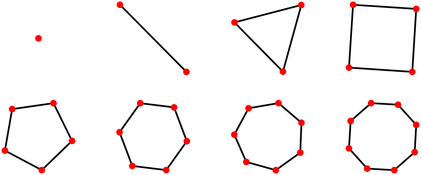
We let to be all simple cycles of size at most 8. This variant of GHC cannot distinguish iso-spectral graphs. The -th dimensional of the embedding vector is
With this configuration, GHC-Tree() has 13 dimensions and GHC-Cycle() has 7 dimensions.
Other methods
To compare our performance with other approaches, we selected some representative methods. GIN (Xu et al., 2019) and PATCHY-SAN (Niepert et al., 2016) are representative of neural-based methods. WL-kernel (Shervashidze et al., 2011) is a widely used efficient method for graph classifications. GNTK (Du et al., 2019) is a recent neural tangent approach to graph classification. We also include results for Ring-GNN (Chen et al., 2019) as this recent model used in theoretical studies performed well in the Circular Skip Links synthetic dataset (Murphy et al., 2019). Except for setting the number of epochs for GIN to be 50, we use the default hyperparameters provided by the original papers. More details for hyperparamters tuning and source code is available in the Supplementary Materials.
4.2 Synthetic Experiments
Bipartite classification
We generate a binary classification problem consisting of 200 graphs, half of which are random bipartite graphs with density and the other half are Erdős-Rényi graphs with density . These graphs have from 40 to 100 vertices. According to Table 1, GHC-Cycle should work well in this case while GHC-Tree can not learn which graph is bipartite. More interestingly, as shown in Table 2, other practical models also can not work with this simple classification problem due to their capability limitation (1-WL).
Circular Skip Links
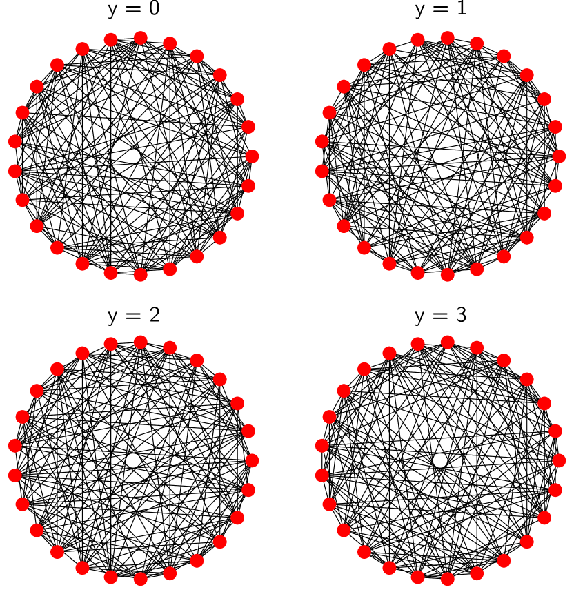
We adapt the synthetic dataset used by (Murphy et al., 2019) and (Chen et al., 2019) to demonstrate another case where GIN, Relational Pooling (Murphy et al., 2019), and Order 2 G-invariant (Maron et al., 2018) do not perform well. Circular Skip Links (CSL) graphs are undirected regular graphs with the same degree sequence (4’s). Since these graphs are not cospectral, GHC-Cycle can easily learn them with 100% accuracy. Chen et al. mentioned that the performance of GNN models could vary due to randomness (accuracies ranging from 10% to 80%). However, it is not the case for GHC-Cycle. CSL classification results shows another benefit of using patterns as an inductive bias to implement a strong classifier without the need of additional features like Ring-GNN-SVD (Chen et al., 2019).
Paulus graphs
We prepare 14 non-isomorphic cospectral strongly regular graphs known as the Paulus graphs777https://www.distanceregular.org/graphs/paulus25.html and create a dataset of 210 graphs belonging to 14 isomorphic groups. This is a hard example because these graphs have exactly the same degree sequence and spectrum. In our experiments, no method achieves accuracy higher than random guesses (7.14%). This is a case when exact isomorphism tests clearly outperform learning-based methods. In our experiments, homomorphisms up to graph index 100 of NetworkX’s graph atlas still fail to distinguish these isomorphic classes. We believe further studies of this case could be fruitful to understand and improve graph learning.
4.3 Benchmark Experiments
We select 3 datasets from the TU Dortmund data collection (Kersting et al., 2016): MUTAG dataset (Debnath et al., 1991), IMDB-BINARY, and IMDB-MULTI (Yanardag & Vishwanathan, 2015). These datasets represent with and without vertex features graph classification settings. We run and record the 10-folds cross-validation score for each experiment. We report the average accuracy and standard deviation of 10 experiments in Table 2. More experiments on other datasets in the TU Dortmund data collection, as well as the details of each dataset, are provided in the Appendix.
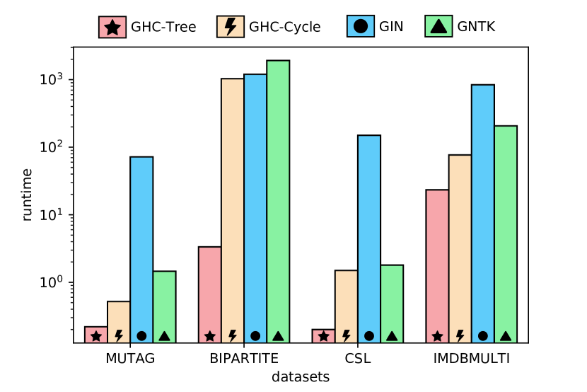
4.4 Running time
Although homomorphism counting is #P-complete in general, polynomial and linear time algorithms exist under the bounded tree-width condition (Díaz et al., 2002). Figure 2 shows that our method runs much faster than other practical models. The results are recorded from averaging total runtime in seconds for 10 experiments, each computes the 10-folds cross-validation accuracy score. In principle, GHC can be linearly distributed to multiple processes to further reduce the computational time making it an ideal baseline model for future studies.
5 Conclusion
In this work we contribute an alternative approach to the question of quantifying a graph classification model’s capability beyond the tensorization order and the Weisfeiler-Lehman isomorphism test. In principle, tensorized graph neural networks can implement homomorphism numbers, hence our work is in coherence with prior work. However, we find that the homomorphism from to is a more “fine-grained” tool to analyze graph classification problems as studying would be more intuitive (and graph-specific) than studying the tensorization order. Since GHC is a more restricted embedding compared to tensorized graph neural networks such as the model proposed by (Keriven & Peyré, 2019), the universality result of GHC can be translated to the universality result of any other model that has the capability to implement the homomorphism numbers.
Another note is about the proof for Theorem 8 (universality on unbounded graphs). In order to prove this result, we made an assumption about the topology of and also about the graph of interest belongs to the graphon space. While the graphon space is natural in our application to prove the universality, there are a few concerns. First, we assumed that the graphons exist for graphs of interest. However, it might not be true in general. Second, graph limit theory is well-studied in dense graphs while sparse graph problems remain largely open.
Acknowledgement
HN is supported by the Japanese Government Scholarship (Monbukagakusho: MEXT SGU 205144). We would like to thank the anonymous reviewers whose comments have helped improving the quality of our manuscript. We thank Jean-Philippe Vert for the helpful discussion and suggestions on our early results. We thank Matthias Springer, Sunil Kumar Maurya, and Jonathon Tanks for proof-reading our manuscripts.
References
- Barabási et al. (2016) Barabási, A.-L. et al. Network science. Cambridge university press, 2016.
- Benson et al. (2016) Benson, A. R., Gleich, D. F., and Leskovec, J. Higher-order organization of complex networks. Science, 353(6295):163–166, 2016.
- Böker et al. (2019) Böker, J., Chen, Y., Grohe, M., and Rattan, G. The complexity of homomorphism indistinguishability. In 44th International Symposium on Mathematical Foundations of Computer Science (MFCS’19), 2019.
- Borgs et al. (2008) Borgs, C., Chayes, J. T., Lovász, L., Sós, V. T., and Vesztergombi, K. Convergent sequences of dense graphs i: Subgraph frequencies, metric properties and testing. Advances in Mathematics, 219(6):1801–1851, 2008.
- Borgwardt et al. (2005) Borgwardt, K. M., Ong, C. S., Schönauer, S., Vishwanathan, S., Smola, A. J., and Kriegel, H.-P. Protein function prediction via graph kernels. Bioinformatics, 21(suppl_1):i47–i56, 2005.
- Bronstein et al. (2017) Bronstein, M. M., Bruna, J., LeCun, Y., Szlam, A., and Vandergheynst, P. Geometric deep learning: going beyond euclidean data. IEEE Signal Processing Magazine, 34(4):18–42, 2017.
- Cai & Govorov (2019) Cai, J.-Y. and Govorov, A. On a theorem of lovász that determines the isomorhphism type of . arXiv preprint arXiv:1909.03693, 2019.
- Chen et al. (2019) Chen, Z., Villar, S., Chen, L., and Bruna, J. On the equivalence between graph isomorphism testing and function approximation with gnns. In Advances in Neural Information Processing Systems, pp. 15868–15876, 2019.
- Collins & Duffy (2002) Collins, M. and Duffy, N. Convolution kernels for natural language. In Advances in Neural Information Processing Systems, pp. 625–632, 2002.
- Debnath et al. (1991) Debnath, A. K., Lopez de Compadre, R. L., Debnath, G., Shusterman, A. J., and Hansch, C. Structure-activity relationship of mutagenic aromatic and heteroaromatic nitro compounds. correlation with molecular orbital energies and hydrophobicity. Journal of medicinal chemistry, 34(2):786–797, 1991.
- Dell et al. (2018) Dell, H., Grohe, M., and Rattan, G. Lovász meets weisfeiler and leman. In Proceedings of the 45th International Colloquium on Automata, Languages, and Programming (ICALP’18), 2018.
- Díaz et al. (2002) Díaz, J., Serna, M., and Thilikos, D. M. Counting h-colorings of partial k-trees. Theoretical Computer Science, 281(1-2):291–309, 2002.
- Du et al. (2019) Du, S. S., Hou, K., Póczos, B., Salakhutdinov, R., Wang, R., and Xu, K. Graph neural tangent kernel: Fusing graph neural networks with graph kernels. CoRR, abs/1905.13192, 2019.
- Fey et al. (2018) Fey, M., Lenssen, J. E., Weichert, F., and Müller, H. SplineCNN: Fast geometric deep learning with continuous B-spline kernels. In IEEE Conference on Computer Vision and Pattern Recognition (CVPR), 2018.
- Flum & Grohe (2006) Flum, J. and Grohe, M. Parameterized Complexity Theory. Springer, 2006.
- Freedman et al. (2007) Freedman, M., Lovász, L., and Schrijver, A. Reflection positivity, rank connectivity, and homomorphism of graphs. Journal of the American Mathematical Society, 20(1):37–51, 2007.
- Gärtner (2003) Gärtner, T. A survey of kernels for structured data. ACM SIGKDD Explorations Newsletter, 5(1):49–58, 2003.
- Gärtner et al. (2003) Gärtner, T., Flach, P., and Wrobel, S. On graph kernels: Hardness results and efficient alternatives. In Learning theory and kernel machines, pp. 129–143. Springer, 2003.
- Gilmer et al. (2017) Gilmer, J., Schoenholz, S. S., Riley, P. F., Vinyals, O., and Dahl, G. E. Neural message passing for quantum chemistry. In Proceedings of the 34th International Conference on Machine Learning, volume 70, pp. 1263–1272. JMLR, 2017.
- Hamilton et al. (2017) Hamilton, W., Ying, Z., and Leskovec, J. Inductive representation learning on large graphs. In Advances in Neural Information Processing Systems, pp. 1024–1034, 2017.
- Hart et al. (2003) Hart, K. P., Nagata, J.-i., and Vaughan, J. E. Encyclopedia of general topology. Elsevier, 2003.
- Haussler (1999) Haussler, D. Convolution kernels on discrete structures. Technical report, Technical report, Department of Computer Science, University of California …, 1999.
- Hell & Nesetril (2004) Hell, P. and Nesetril, J. Graphs and homomorphisms. Oxford University Press, 2004.
- Keriven & Peyré (2019) Keriven, N. and Peyré, G. Universal invariant and equivariant graph neural networks. arXiv preprint arXiv:1905.04943, 2019.
- Kersting et al. (2016) Kersting, K., Kriege, N. M., Morris, C., Mutzel, P., and Neumann, M. Benchmark data sets for graph kernels, 2016. URL http://graphkernels.cs.tu-dortmund.de.
- Kriege et al. (2016) Kriege, N. M., Giscard, P.-L., and Wilson, R. On valid optimal assignment kernels and applications to graph classification. In Advances in Neural Information Processing Systems, pp. 1623–1631, 2016.
- Kriege et al. (2019) Kriege, N. M., Johansson, F. D., and Morris, C. A survey on graph kernels. arXiv preprint arXiv:1903.11835, 2019.
- Lovász (1967) Lovász, L. Operations with structures. Acta Mathematica Hungarica, 18(3-4):321–328, 1967.
- Lovász (2012) Lovász, L. Large networks and graph limits, volume 60. American Mathematical Soc., 2012.
- Lovász & Szegedy (2006) Lovász, L. and Szegedy, B. Limits of dense graph sequences. Journal of Combinatorial Theory, Series B, 96(6):933–957, 2006.
- Mahé & Vert (2009) Mahé, P. and Vert, J.-P. Graph kernels based on tree patterns for molecules. Machine learning, 75(1):3–35, 2009.
- Maron et al. (2018) Maron, H., Ben-Hamu, H., Shamir, N., and Lipman, Y. Invariant and equivariant graph networks. arXiv preprint arXiv:1812.09902, 2018.
- Maron et al. (2019) Maron, H., Fetaya, E., Segol, N., and Lipman, Y. On the universality of invariant networks. arXiv preprint arXiv:1901.09342, 2019.
- Mezentsev (2004) Mezentsev, A. A. A generalized graph-theoretic mesh optimization model. In IMR, pp. 255–264, 2004.
- Milo et al. (2002) Milo, R., Shen-Orr, S., Itzkovitz, S., Kashtan, N., Chklovskii, D., and Alon, U. Network motifs: simple building blocks of complex networks. Science, 298(5594):824–827, 2002.
- Morris et al. (2019) Morris, C., Ritzert, M., Fey, M., Hamilton, W. L., Lenssen, J. E., Rattan, G., and Grohe, M. Weisfeiler and leman go neural: Higher-order graph neural networks. In Proceedings of the AAAI Conference on Artificial Intelligence, volume 33, pp. 4602–4609, 2019.
- Murphy et al. (2019) Murphy, R., Srinivasan, B., Rao, V., and Ribeiro, B. Relational pooling for graph representations. In Chaudhuri, K. and Salakhutdinov, R. (eds.), Proceedings of the 36th International Conference on Machine Learning, volume 97 of Proceedings of Machine Learning Research, pp. 4663–4673, Long Beach, California, USA, 09–15 Jun 2019. PMLR.
- Niepert et al. (2016) Niepert, M., Ahmed, M., and Kutzkov, K. Learning convolutional neural networks for graphs. In International conference on machine learning, pp. 2014–2023, 2016.
- Pržulj et al. (2004) Pržulj, N., Corneil, D. G., and Jurisica, I. Modeling interactome: scale-free or geometric? Bioinformatics, 20(18):3508–3515, 2004.
- Robertson & Seymour (1986) Robertson, N. and Seymour, P. D. Graph minors. ii. algorithmic aspects of tree-width. Journal of algorithms, 7(3):309–322, 1986.
- Sannai et al. (2019) Sannai, A., Takai, Y., and Cordonnier, M. Universal approximations of permutation invariant/equivariant functions by deep neural networks. arXiv preprint arXiv:1903.01939, 2019.
- Shervashidze et al. (2009) Shervashidze, N., Vishwanathan, S., Petri, T., Mehlhorn, K., and Borgwardt, K. Efficient graphlet kernels for large graph comparison. In Artificial Intelligence and Statistics, pp. 488–495, 2009.
- Shervashidze et al. (2011) Shervashidze, N., Schweitzer, P., Leeuwen, E. J. v., Mehlhorn, K., and Borgwardt, K. M. Weisfeiler-lehman graph kernels. Journal of Machine Learning Research, 12(Sep):2539–2561, 2011.
- Togninalli et al. (2019) Togninalli, M., Ghisu, E., Llinares-López, F., Rieck, B., and Borgwardt, K. Wasserstein weisfeiler-lehman graph kernels. arXiv preprint arXiv:1906.01277, 2019.
- Wu et al. (2019) Wu, Z., Pan, S., Chen, F., Long, G., Zhang, C., and Yu, P. S. A comprehensive survey on graph neural networks. arXiv preprint arXiv:1901.00596, 2019.
- Xu et al. (2019) Xu, K., Hu, W., Leskovec, J., and Jegelka, S. How powerful are graph neural networks? International Conference on Learning Representations, 2019.
- Yanardag & Vishwanathan (2015) Yanardag, P. and Vishwanathan, S. Deep graph kernels. In Proceedings of the 21th ACM SIGKDD International Conference on Knowledge Discovery and Data Mining, pp. 1365–1374, 2015.
APPENDIX
A Implementation Details
The source code for GHC is provided with this supplementary document. The main implementation is in file homomorphism.py. Aside from Algorithm 1, which can be implemented directly with numpy and run with networkx, other types of homomorphism counting are implemented with C++ and called from homomorphism.py. The implementation for general homomorphism is called homlib. We include an instruction to install homlib in its README.md. All our experiments are run on a PC with the following specifications. Kernel: 5.3.11-arch1-1; CPU: Intel i7-8700K (12) 4.7 GHz; GPU: NVIDIA GEFORCE GTX 1080 Ti 11GB; Memory: 64 GB. Note that GPU is only used for training GIN (Xu et al., 2019).
Benchmark Experiments
The main file to run experiment on real-world (benchmark) datasets is tud.py. This is a simple classification problem where each graph in a dataset belongs to a single class. While any other classifier can be used with GHC, we provide the implementation only for Support Vector Machines (scikit-learn) with One-Versus-All multi-class algorithm. We preprocess the data using the StandardScaler provided with scikit-learn. As described in the main part of this paper, we report the best 10-folds cross validation accuracy scores across different SVM configurations. The parameter settings for this experiments are:
-
•
Homomorphism types: Tree, LabelTree (weighted homomorphism), and Cycle.
-
•
Homomorphism size: 6 for trees and 8 for cycles. Theoretically, the homomorphism size increase implies performance increase, but in practice we observe no improvement in classification accuracy beyond size 6. The number of non-isomorphic trees of size is presented in Table 9.
-
•
SVC kernel: Radial Basis Function, Polynomial (max degree = 3).
-
•
SVC regularization parameter (C): values in the log-space from to .
-
•
SVC kernel coefficient (gamma): ‘scale’ (1 / (n_features * X.var())
| 2 | 3 | 4 | 5 | 6 | 7 | 8 | |
|---|---|---|---|---|---|---|---|
| # trees | 1 | 1 | 2 | 3 | 6 | 11 | 23 |
| 9 | 10 | 11 | 12 | 13 | 14 | 15 | |
| # trees | 47 | 106 | 235 | 551 | 1301 | 3159 | 7741 |
Synthetic Experiments
The main file to run experiment on real-world (benchmark) datasets is synthetic.py and the implementation of synthetic datasets can be found in utils.py. Since these experiments focus on the capability of GHC, we can achieve the best performance with just a simple classifier. The parameter settings for this experiments are:
-
•
Homomorphism types: Tree and Cycle.
-
•
Homomorphism size: 6 for trees and 8 for cycles.
-
•
SVC kernel: Radial Basis Function.
-
•
SVC regularization parameter (C): Fix at .
-
•
SVC kernel coefficient (gamma): Fix at .
We provide in our source code helper functions which behave the same as the default dataloader used by GIN and GNTK implementations. The external loaders are provided in externals.py. Users can copy-paste (or import) these loader into the repository provided by GIN and GNTK to run our synthetic experiments. The settings for other models are set as in the benchmark experiments.
Timing Experiments
We measure run-time using the time module provided with Python 3.7. The reported time in Figure 2 is the total run-time (in seconds) including homomorphism time and prediction time for our model as well as kernel learning time and prediction time for others.
B Datasets
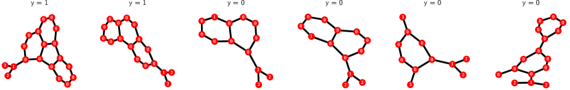
As other works in the literature, we use the TU Dortmund data collections (Kersting et al., 2016). The overview of these datasets are provided in Table 4. We provide additional classification results for these datasets in Table 5 and Table 6. We also provide some example of MUTAG data in Figure 4, four first isomorphic groups of PAULUS25 in Figure 3, plot of trees and cycles used in GHC-Tree (Figure 5 and GHC-Cycles (Figure 6).
| Datasets | |||||
|---|---|---|---|---|---|
| MUTAG | 188 | 17.9 | 2 | no | yes |
| PTC-MR | 344 | 25.5 | 2 | no | yes |
| NCI1 | 4110 | 29.8 | 2 | no | yes |
| PROTEINS | 1113 | 39.1 | 2 | yes | yes |
| D&D | 1178 | 284.3 | 2 | no | yes |
| BZR | 405 | 35.7 | 2 | yes | yes |
| RDT-BIN | 2000 | 429.6 | 2 | no | no |
| RDT-5K | 5000 | 508.5 | 5 | no | no |
| RDT-12K | 11929 | 391.4 | 11 | no | no |
| COLLAB | 5000 | 74.5 | 3 | no | no |
| IMDB-BIN | 1000 | 19.8 | 2 | no | no |
| IMDB-MUL | 1500 | 13.0 | 3 | no | no |
| Bipartite | 200 | 70.0 | 2 | no | no |
| CSL | 150 | 41.0 | 10 | no | no |
| Paulus 25 | 210 | 25.0 | 14 | no | no |
| Methods | Datasets | |||||
|---|---|---|---|---|---|---|
| RDT-BIN | RDT-5K | RDT-12K | COLLAB | IMDB-BIN | IMDB-MUL | |
| Our experiments (Average over 10 runs of stratified 10-folds CV) | ||||||
| GHC-Tree | 88.42 2.05 | 52.98 1.83 | 44.8 1.00 | 75.23 1.71 | 72.10 2.62 | 48.60 4.40 |
| GHC-Cycles | 87.61 2.45 | 52.45 1.24 | 40.9 2.01 | 72.59 2.02 | 70.93 4.54 | 47.61 3.67 |
| GIN | 74.10 2.34 | 46.74 3.07 | 32.56 5.33 | 75.90 0.81 | 70.70 1.1 | 43.20 2.00 |
| GNTK | - | - | - | 83.70 1.00 | 75.61 3.98 | 51.91 3.56 |
| Literature (One run of stratified 10-folds CV) | ||||||
| GIN | 92.4 2.5 | 57.5 1.5 | - | 80.2 1.9 | 75.1 5.1 | 52.3 2.8 |
| PATCHY-SAN | 86.3 1.6 | 49.1 0.7 | - | 72.6 2.2 | 71.0 2.2 | 45.2 2.8 |
| WL kernel | 80.8 0.4 | - | - | 79.1 0.1 | 73.12 0.4 | - |
| Graphlet kernel | 60.1 0.2 | - | 31.8 | 64.7 0.1 | - | - |
| AWL kernel | 87.9 2.5 | 54.7 2.9 | - | 73.9 1.9 | 74.5 5.9 | 51.5 3.6 |
| WL-OA kernel | 89.3 | - | - | 80.7 0.1 | - | - |
| WL-W kernel | - | - | - | - | 74.37 0.83 | - |
| GNTK | - | - | - | 83.6 1.0 | 76.9 3.6 | 52.8 4.6 |
| Methods | Datasets | |||||
|---|---|---|---|---|---|---|
| MUTAG | PTC-MR | NCI1 | PROTEINS | D&D | BZR | |
| Our experiments (Average over 10 runs of stratified 10-folds CV) | ||||||
| GHC-Tree | 89.28 8.26 | 52.98 1.83 | 48.8 1.00 | 75.23 1.71 | 72.10 2.62 | 48.60 4.40 |
| GHC-Cycle | 87.81 7.46 | 50.97 2.13 | 47.4 1.02 | 74.30 1.93 | 70.10 2.49 | 47.20 3.84 |
| GHC-LabelTree | 88.86 4.82 | 59.68 7.98 | 73.95 1.99 | 73.27 4.17 | 76.50 3.15 | 82.82 4.37 |
| GIN | 74.10 2.34 | 46.74 3.07 | 76.67 1.16 | 75.9 0.81 | 70.70 1.1 | 43.20 2.00 |
| GNTK | 89.65 7.5 | 68.2 5.8 | 85.0 1.2 | 76.60 5.02 | 75.61 3.98 | 83.64 2.95 |
| Literature (One run of stratified 10-folds CV) | ||||||
| GIN | 89.4 5.6 | 64.6 7.0 | 82.7 1.7 | 76.2 2.8 | - | - |
| PATCHY-SAN | 92.5 4.2 | 60.0 4.8 | 78.6 1.9 | 75.9 2.8 | 77.12 2.41 | - |
| WL kernel | 90.4 5.7 | 59.9 4.3 | 86.0 1.8 | 75.0 3.1 | 79.78 0.36 | 78.59 0.63 |
| Graphlet kernel | 85.2 0.9 | 54.7 2.0 | 70.5 0.2 | 72.7 0.6 | 79.7 0.7 | - |
| AWL kernel | 87.9 9.8 | - | - | - | - | - |
| WL-OA kernel | 84.5 0.17 | 63.6 1.5 | 86.1 0.2 | 76.4 0.4 | 79.2 0.4 | - |
| WL-W kernel | 87.27 1.5 | 66.31 1.21 | 85.75 0.25 | 77.91 0.8 | 79.69 0.50 | 84.42 2.03 |
| GNTK | 90.00 8.5 | 67.9 6.9 | 84.2 1.5 | 75.6 4.2 | - | - |
Remark 22.
We conjecture that the above result can be extended to the infinite graphs (say, graphons).