Effective lockdown and role of hospital-based COVID-19 transmission in some Indian states: An outbreak risk analysis

Abstract

There are several reports in India that indicate hospitals and quarantined centers are COVID-19 hotspots. In the absence of efficient contact tracing tools, Govt. and the policymakers may not be paying attention to the risk of hospital-based transmission. To explore more on this important route and its possible impact on lockdown effect, we developed a mechanistic model with hospital-based transmission. Using daily notified COVID-19 cases from six states (Maharashtra, Delhi, Madhya Pradesh, Rajasthan, Gujarat, and Uttar Pradesh) and overall India, we estimated several important parameters of the model. Moreover, we provided an estimation of the basic ($R_{0}$), the community ($R_{C}$), and the hospital ($R_{H}$) reproduction numbers for those seven locations. To obtain a reliable forecast of future COVID-19 cases, a BMA post-processing technique is used to ensemble the mechanistic model with a hybrid statistical model. Using the ensemble model, we forecast COVID-19 notified cases (daily and cumulative) from May 3, 2020, till May 20, 2020, under five different lockdown scenarios in the mentioned locations. Our analysis of the mechanistic model suggests that most of the new COVID-19 cases are currently undetected in the mentioned seven locations. Furthermore, a global sensitivity analysis of four epidemiologically measurable & controllable parameters on $R_{0}$ and as well on the lockdown effect, indicate that if appropriate preventive measures are not taken immediately, a much larger COVID-19 outbreak may trigger from hospitals and quarantined centers. In most of the locations, our ensemble model forecast indicates a substantial percentage of increase in the COVID-19 notified cases in the coming weeks in India. Based on our results, we proposed a containment policy that may reduce the threat of a larger COVID-19 outbreak in the coming days.

Introduction

Coronavirus disease of 2019 (COVID-19) was first observed in Wuhan, China and rapidly spread across the globe in a short duration Chen2020Lancet . World Health Organization (WHO) declares COVID-19 as pandemic after assessing its various characteristics WHO_Pandemic . As of April 29, 2020–over three million cases and over two hundred thousand deaths due to COVID-19 is reported across the globe worldcovid2020track . In India, the first confirmed case of COVID-19 was reported on $30/01/2020$ WHO2020_1 , a student from Kerala studying in a university in Wuhan India_Today5 . As of April 29, 2020–$33065$ confirmed cases and $1079$ deaths due to COVID-19 are reported in India indiacovid2020track .

According to a daily monitoring report published by WHO, $22,073$ healthcare workers across $52$ countries are being tested positive to COVID-19 WHOreportheathcare2020 . The report also noted that the number provided may be an underestimation as there is no systematic reporting of infections among the healthcare workers WHOreportheathcare2020 . In India, there are several reports that indicate hospitals and quarantined centers are COVID-19 hotspots TheHINDUsuperspreaders ; India_Today1 ; Economic_Times1 ; Print_In1 ; NDTV2 . The doctors, nurses and other health workers are mainly vulnerable as they are in close proximity with the COVID-19 patients India_Today1 ; Economic_Times1 ; Print_In1 ; NDTV2 ; NDTVheathcareworkers . The close relatives of the notified COVID-19 patients in the quarantine centers may also be at risk of getting infection. In addition, those journalists who are continuously visiting hospitals and quarantine centers to get updated reports on COVID-19, may also be at risk of getting infection IndiaTVjournalistscovid19 ; Scroll_In1 . Therefore, a significant percentage of susceptible population in the community may be exposed to COVID-19 infection occurring from the contacts with patents in hospitals and quarantine centers. Due to unavailability of efficient contact tracing tools, Govt. and the policy makers may be ignoring this important transmission route of COVID-19.

Currently there is no vaccine and effective medicine available for COVID-19. Therefore, to break the transmission chain of COVID-19, Govt. had implemented a full nation-wise lockdown (home quarantined the community) staring from March 25, 2020 till April, 14, 2020. However, the large country like India with such diverse and huge population, lockdown all over the nation may not be a very feasible and effective solution. In addition, lockdown already have a huge impact on the Indian economy specially on the short scale industries Economic_Times2 ; India_Today4 . To partially overcome this economic crisis as well reducing COVID-19 transmission, Govt. has proposed some amendments (known as cluster containment strategy) on the lockdown rules from April 20, 2020 Economictimes2020a ; financialexpress20a . In these revised rules, Govt. has provided some relaxation in current rules by dividing different districts of the various states into three zones namely red (hotspot), orange (limited human movement), and green (economic activity) depending on the number of COVID-19 cases Economictimes2020a ; financialexpress20a ; businesstoday2020a . However, question remains whether this cluster containment strategy may be successful in reducing COVID-19 transmission or not? If not then what may be other alternative solutions to reduce COVID-19 transmission? These question can only be answered by studying the dynamics and prediction of a mechanistic mathematical model for COVID-19 transmission and testing the results in real situation.

Mechanistic mathematical models based on system of ordinary differential equations (ODE) may provide useful information regarding transmission dynamics of COVID-19 and its control. Recently, there are several modeling studies that provide information on different effective control measures for reducing COVID-19 transmission Moghadas2020PNAS ; Tang2020 ; sardar2020assessment . In their study, Moghdas et al Moghadas2020PNAS developed an age-structure model on COVID-19 and projected required ICU beds for different outbreak scenarios in USA. To improve the hospital capacity and possible containment of COVID-19, they recommended self isolation and better hygiene practices in the community. Using a mechanistic model, Tang et al Tang2020 estimated the control reproduction numbers and studied the effect of various interventions on COVID-19 transmission in China. Recently, Sardar et al sardar2020assessment provided an effective lockdown strategy to control COVID-19 transmission in India. They recommended cluster specific lockdown policy in different parts of India for effective reduction in transmission of COVID-19. There are some recent studies that uses different statistical modeling techniques to provide reliable real-time forecast of COVID-19 cases Chakraborty2020Arxiv ; Tandon2020Arxiv ; Hu2020Arxiv . Therefore, a combination of mathematical and statistical models may be effective in determining the control measures as well providing a robust real-time forecast of future COVID-19 cases and deaths in different parts of India and for other countries as well.

In this paper, we formulated a mechanistic model with hospital-based transmission. We assume that COVID-19 patients from the hospitals and quarantine centers can only be in contact with a small fraction of the susceptible population from the community. Furthermore, we assume different transmission rates for the community and the hospital-based infection. In the mechanistic model, we have incorporated the lockdown effect through home quarantine of a certain percentage of susceptible population from the community. Using daily notified COVID-19 cases from six states (Maharashtra, Delhi, Madhya Pradesh, Rajasthan, Gujarat, and Uttar Pradesh) and overall India, we estimated several important parameters of the mechanistic model. Furthermore, we estimated the basic ($R_{0}$), the community ($R_{C}$), and the hospital ($R_{H}$) reproduction numbers for the seven locations under study. To obtain a reliable forecast of future COVID-19 notified cases in the above mentioned locations, we used a hybrid statistical model that can efficiently capture fluctuations in the daily time series data. BMA post-processing technique based on DRAM algorithm is used to ensemble our mechanistic mathematical model with the hybrid statistical model. Using the ensemble model, we forecast COVID-19 notified cases (daily and cumulative) from May 3, 2020 to May 20, 2020, under five different lockdown scenarios in the seven locations. To determine an effective lockdown policy, we carried out a global sensitivity analysis of four epidemiologically measurable & controllable parameters on the lockdown effect (number of cases reduction) and as well on $R_{0}$.

Method

We extend a previous mechanistic model sardar2020assessment by considering hospital-based COVID-19 transmission (see Fig 1 and supplementary). We assume that hospitalized & notified infected population can only be in contact with a small fraction ($\rho$) of the susceptible population from the community (see Table 1 and supplementary). We assume different transmission rates ($\beta_{1}$ and $\beta_{2}$, respectively) for community and hospital-based infection. As it is very difficult to detect asymptomatic infected in the community therefore, we assume that only a fraction of symptomatic infected population being notified & hospitalized by COVID-19 testing at a rate, $\tau$ (see Fig 1 and Table 1). Following sardar2020assessment , the disease related deaths are considered only for the notified & hospitalized population at a rate $\delta$. We incorporated lockdown effect in our model (see Fig 1 and supplementary) by home quarantined a fraction of susceptible population at a rate $l$. We also assume that after the current lockdown period $\left(\displaystyle\frac{1}{\omega}=40\hskip 2.84544ptdays\right)$ the home quarantined individuals will returned to the general susceptible population (see Fig 1 and supplementary). Moreover, we assume that the home quarantined individuals do not mixed with the general population (see Fig 1) i.e. this class of individuals do not contribute in the disease transmission. A flow diagram and the information on our mechanistic ODE model parameters are provided in Fig 1 and Table 1, respectively.

Mechanistic ODE model (see Fig 1 and supplementary) we are using for this study may be efficient in capturing overall trend of the time-series data and the transmission dynamics of COVID-19. However, as solution of the ODE model is always smooth therefore, our mechanistic model may not be able to capture fluctuations occurring in the daily time-series data. Several complex factors like lockdown, symptomatic, asymptomatic, hospital transmission, awareness, rapid testing, preventive measures, etc may influence the variations in daily COVID-19 time-series data. Therefore, it is an extremely challenging job to fit and long term forecast using this daily time-series data. To resolve this issue, we considered a Hybrid statistical model which is a combination of five forecasting models namely, Auto-regressive Integrated Moving Average model (ARIMA); Exponential smoothing state space model (ETS); Theta Method Model (THETAM); Exponential smoothing state space model with Box-Cox transformation, ARMA errors, Trend and Seasonal components (TBATS); and Neural Network Time Series Forecasts (NNETAR). Finally, the Hybrid statistical model and the mechanistic ODE model (see Fig 1 and supplementary) are combined together by a post-processing Bayesian Model Averaging (BMA) technique which we discussed later in the manuscript.

We used daily confirmed COVID-19 cases from Maharashtra (MH), Delhi (DL), Madhya Pradesh (MP), Rajasthan (RJ), Gujarat (GJ), Uttar Pradesh (UP) and overall India (IND) for the time period March 14, 2020 to April 14, 2020 (MH), March 14, 2020 to April 18, 2020 (DL), March 20, 2020 to April 17, 2020 (MP), March 14, 2020 to April 18, 2020 (RJ), March 19, 2020 to April 16, 2020 (GJ), March 14, 2020 to April 18, 2020 (UP), and March 2, 2020 to April 19, 2020 (IND) for our study. As of April 29, 2020, these referred six states contributes 74% of the total COVID-19 notified cases in India indiacovid2020track . Confirmed daily COVID-19 cases form these mentioned seven locations are collected from indiacovid2020track . State-wise population data are taken from aadhaar20 .

We estimated several uninformative parameters (see Table 1) of our mechanistic model (see Fig 1 and supplementary) by calibrating our mathematical model (see Fig 1 and supplementary) to the daily notified COVID-19 cases from the seven locations MH, DL, MP, RJ, GJ, UP, and IND respectively. As some initial conditions of our mathematical model (see Fig 1 and supplementary) are also unknown therefore, we prefer to estimate these uninformative initial conditions from the data (see Table S1 in supplementary). In lockdown 1.0, the Indian Govt. has implemented a 21 days nationwide full lockdown (home quarantined the community) starting from March 25, 2020 to April 14, 2020 Economictimes2020 and Govt. then extend the lockdown period up to May 3, 2020 (lockdown 2.0) timesofindia20b ; financialexpress20 . Therefore, the daily COVID-19 time series data contains the effect of with and without lockdown scenario, therefore, we prefer to use a combination of two mathematical models (without and with lockdown) for calibration. An elaboration on the combination technique of the mathematical models without and with lockdown (see Fig 1 and supplementary) is provided below:

$\bullet$

We first use the mechanistic model without lockdown (see Eq S1 in supplementary) starting from the first date of the daily COVID-19 data up to end of March 24, 2020 for the seven locations MH, DL, MP, RJ, GJ, UP, and IND, respectively.

$\bullet$

Using values of the state variables of the model without lockdown (see Model S1 in supplementary method) onset of March 24, 2020 as initial conditions, we run the mechanistic model with lockdown (see Fig 1 and Model S2 in supplementary) up to the end date of the daily COVID-19 data for the seven locations MH, DL, MP, RJ, GJ, UP, and IND, respectively.

The nonlinear least square function ${}^{\prime}lsqnonlin^{\prime}$ in the MATLAB based optimization toolbox is called to fit the simulated and observed daily COVID-19 notified cases in those seven locations mentioned earlier. Bayesian based ${}^{\prime}DRAM^{\prime}$ algorithm haario2006dram is used to sample the uninformative parameters and initial conditions (see Table S1 and Table S2 in supplementary) of the mathematical models combination without and with lockdown (see Fig 1 and supplementary). A details on mechanistic model fitting is provided in sardar2017mathematical .

Calibration of the Hybrid statistical model for the mentioned seven states are done using the $R$ package ${}^{\prime}forecastHybrid^{\prime}$. First, we fitted the individual models ARIMA, ETS, THETAM, TBATS, and NNETAR by calling the functions ${}^{\prime}auto.arima^{\prime}$, ${}^{\prime}ets^{\prime}$, ${}^{\prime}thetam^{\prime}$, ${}^{\prime}tbats^{\prime}$, and ${}^{\prime}nnetar^{\prime}$ respectively. The results generated from each of the above models are combined with equal weights to determine the Hybrid statistical model. Equal weight among the five individual models are taken as it generates a robust result (see Table S4 in supplementary) for the Hybrid statistical model lemke2010meta .

Post-processing BMA technique for combining the mechanistic model (see Fig 1 and supplementary) and the Hybrid statistical model is based on ${}^{\prime}DRAM^{\prime}$ algorithm haario2006dram . Let, $\displaystyle Y^{ODE}=\{y_{j}^{ODE}\}_{j=1}^{n}$ and $\displaystyle Y^{HBD}=\{y_{j}^{HBD}\}_{j=1}^{n}$ be $n$ simulated observations from our mechanistic ODE model (see Fig 1 and supplementary) and the Hybrid statistical model respectively and let, $\displaystyle\hat{Y}=\{y_{j}^{obs}\}_{j=1}^{n}$ be $n$ observation from the data. Then

$$Y^{E}=w_{1}\hskip 5.69046ptY^{ODE}+w_{2}\hskip 5.69046ptY^{HBD},$$ (0.1)

is our ensemble model, where, the weights $w_{1}$ and $w_{2}$ satisfies the constraints

$$\Delta=\left\{w_{1},w_{2}\geq 0:w_{1}+w_{2}=1\right\}.$$

We assume $w_{1}$ and $w_{2}$ follows Gaussian proposal distribution. Then the error sum of square function haario2006dram is defined as:

$$SS(\tilde{\theta})=\sum_{i=1}^{n}\left(\hat{Y}-Y^{E}(\tilde{\theta})\right)^{2}.$$

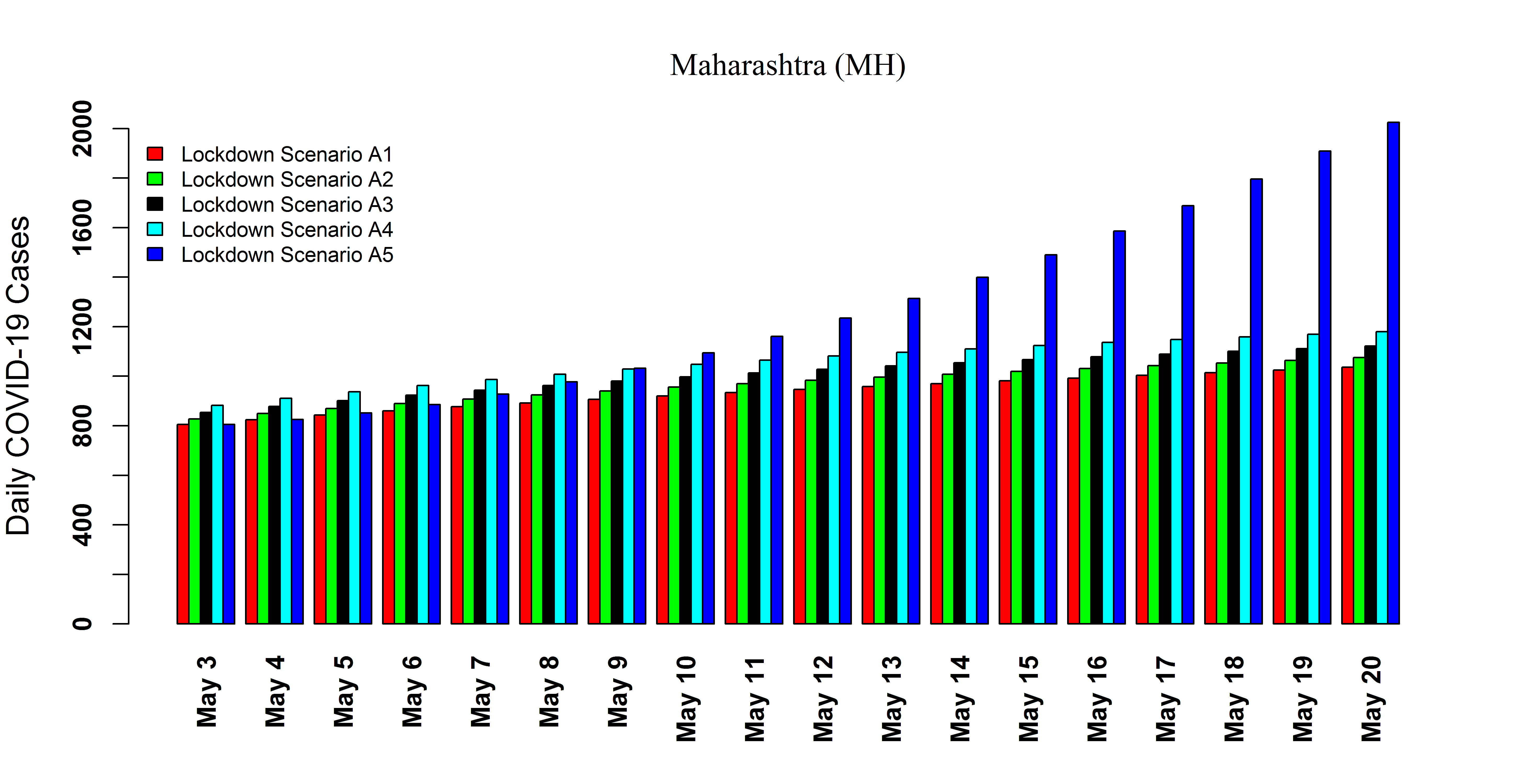
Figure S1: Ensemble model (see main text) forecast for the daily notified COVID-19 cases in Maharashtra during May 3, 2020 till May 20, 2020 under five different lockdown scenarios. Under lockdown scenarios (A2) to (A4), projections are made with 10%, 20% and 30% decrement in the current estimate of the lockdown rate, respectively (see Table 2 in main text). In lockdown scenario (A1), projections are made with current estimated lockdown rate (see Table 2 in main text). Finally, in the lockdown scenario (A5), projections are made with no lockdown during May 3, 2020 till May 20, 2020.

Posterior distribution of the weights $\tilde{\theta}=\left(\tilde{w_{1}},\tilde{w_{2}}\right)$ for the ensemble model (0.1) are generated using Bayesian based ${}^{\prime}DRAM^{\prime}$ algorithm haario2006dram (see Table S3 and Fig S1 to S7 in supplementary).

To save the countries short-scale industries and the agricultural sectors, Indian Govt. has proposed some amendments on current lockdown rules from April 20, 2020 Economictimes2020a ; financialexpress20a . In these revised rules, Govt. has provided some relaxation in current rules by dividing different districts of the various states into three red (hotspot), orange (limited human movement), and green (Economic activity) zones depending on the number of COVID-19 cases Economictimes2020a ; financialexpress20a ; businesstoday2020a . Implementation of these new rules in our mechanistic models combination (see Fig 1 and supplementary) are based on the following assumptions:

$\bullet$

Lockdown rule will be relaxed from April 20, 2020 in those states where the current estimate of the lockdown rate (see Table 2) is higher than a threshold value. This relaxation in lockdown is based on the fact that locations where lockdown are strictly implemented before April 20, 2020 are likely to have more impact on the economic growth.

$\bullet$

Lockdown rule will be more intensive from April 20, 2020 in those states where the current estimate of the lockdown rate (see Table 2) is below a threshold value. This assumption is made because locations where lockdown are not implemented properly before April 20, 2020 are likely to have more red (hotspot) zones.

$\bullet$

50% lockdown success is taken as the threshold value for our study. Here, 50% lockdown success in Delhi means that 50% of the susceptible population in this state is successfully home-quarantined during the period March 25, 2020 till April 20, 2020.

$\bullet$

Insensitivity and relaxation in lockdown are measured in a same scale namely 10%, 20% and 30% increment or decrement on the current estimate of lockdown rate (see Table 2).

Following the above assumptions and using our ensemble model (0.1), we provided a forecast of notified COVID-19 cases (daily and cumulative) for MH, DL, MP, RJ, GJ, UP, and IND, respectively during May 3, 2020 till May 20, 2020. As COVID-19 notified cases are continuously rising in these seven locations therefore, it is more likely that lockdown period will be extended beyond May 3, 2020. Therefore, forecast using the ensemble model (0.1) during the mentioned time duration in those seven locations are based on the following scenarios:
(A1) Using our mechanistic models combination (see Fig 1 and supplementary) and the current estimate of the lockdown rates (see Table 2), we forecast notified COVID-19 cases up to May 20, 2020. This forecast is combined together with the results obtain from the hybrid statistical model by using our ensemble model (0.1).

(A2) Using our mechanistic models combination (see Fig 1 and supplementary) and the current estimate of the lockdown rates (see Table 2), we forecast notified COVID-19 cases up to April 20, 2020. From April 21, 2020 till May 20, 2020, forecast are made using 10% increment or decrement (depending on the state) in the estimate of current lockdown rate. This forecast is combined together with the results obtain from the hybrid statistical model by using our ensemble model (0.1).

(A3) Using our mechanistic models combination (see Fig 1 and supplementary) and the current estimate of the lockdown rates (see Table 2), we forecast notified COVID-19 cases up to April 20, 2020. From April 21, 2020 till May 20, 2020, forecast are made using 20% increment or decrement (depending on the state) in the estimate of current lockdown rate. This forecast is combined together with the results obtain from the hybrid statistical model by using our ensemble model (0.1).

(A4) Using our mechanistic models combination (see Fig 1 and supplementary) and the current estimate of the lockdown rates (see Table 2), we forecast notified COVID-19 cases up to April 20, 2020. From April 21, 2020 till May 20, 2020, forecast are made using 30% increment or decrement (depending on the state) in the estimate of current lockdown rate. This forecast is combined together with the results obtain from the hybrid statistical model by using our ensemble model (0.1).

(A5) Using our mechanistic models combination (see Fig 1 and supplementary) and the current estimate of the lockdown rates (see Table 2), we forecast notified COVID-19 cases up to May 2, 2020. From May 3, 2020 till May 20, 2020, forecast are made with no lockdown (see Eq. S1 in supplementary). This forecast is combined together with the results obtain from the hybrid statistical model by using our ensemble model (0.1).

As, we assumed that lockdown individuals do not mixed with the general population therefore, the basic reproduction number ($R_{0}$) with and without lockdown (see Fig 1 and supplementary) are equal van2002reproduction :

$$R_{0}=\frac{\beta_{1}\kappa\sigma}{(\mu+\sigma)(\gamma_{1}+\mu+\tau)}+\frac{\beta_{1}(1-\kappa)\sigma}{(\mu+\gamma_{2})(\mu+\sigma)}+\frac{\beta_{2}\kappa\rho\sigma\tau}{(\mu+\sigma)(\delta+\gamma_{3}+\mu)(\gamma_{1}+\mu+\tau)}.\\$$

In the expression of $R_{0}$, sum of first two term indicate the community infection occurring from symptomatic and asymptomatic infected population. The third term in $R_{0}$ specify the hospital-based COVID-19 transmission. To distinguish the community and hospital-based COVID-19 transmission, we defined the community reproduction number ($R_{C}$), and the hospital reproduction number ($R_{H}$) as follows:

$$R_{C}=\frac{\beta_{1}\kappa\sigma}{(\mu+\sigma)(\gamma_{1}+\mu+\tau)}+\frac{\beta_{1}(1-\kappa)\sigma}{(\mu+\gamma_{2})(\mu+\sigma)},\\$$

and

$$R_{H}=\frac{\beta_{2}\hskip 1.13791pt\kappa\hskip 1.13791pt\rho\hskip 1.13791pt\sigma\hskip 1.13791pt\tau}{(\mu+\sigma)(\delta+\gamma_{3}+\mu)(\gamma_{1}+\mu+\tau)}.\\$$

Using estimated values of epidemiologically uninformative parameters (see Table 2), we estimated $R_{0}$, $R_{C}$, and $R_{H}$ for the seven locations MH, DL, MP, RJ, GJ, UP, and IND, respectively.

Constructing an effective policy on future lockdown in a region will require some relation between effect of lockdown (number of COVID-19 case reduction) with some important epidemiologically measurable & controllable parameters. Our mechanistic ODE model (see Fig 1 and supplementary) has several important parameters and among them measurable and controllable parameters are $\beta_{2}$: average rate of transmission occurring from hospitalized & notified based contacts (it can be controllable by following WHO guidelines); $\rho$: fraction of susceptible population from the community that are exposed to notified & hospitalized based contacts (it also can be minimized by following proper guidelines from WHO); $\kappa$: fraction of infected that are symptomatic (rapid COVID-19 testing can provide an accurate estimate); $\tau$: notification & hospitalization rate of symptomatic infected population (it also depend on number of COVID-19 testing). We perform a global sensitivity analysis marino2008methodology to determine the effect of these parameters on the lockdown effect and on the basic reproduction number ($R_{0}$), respectively. The effect of lockdown is measured in terms of differences in the total number of COVID-19 cases occurred during May 3, 2020 till May 20, 2020 under the lockdown scenarios (A1) and (A5), respectively. We draw $500$ samples from the biologically feasible ranges of the mentioned four parameters (see Table 1) using Latin Hypercube Sampling (LHS) technique. Other informative and uninformative parameters during simulation of the mechanistic model are taken from Table 1 and Table 2, respectively. Partial rank correlation coefficients (PRCC) and its corresponding $p$-value are evaluated to determine the effect of these mentioned four parameters on the lockdown effect and the basic reproduction number ($R_{0}$), respectively.

Results and Discussion

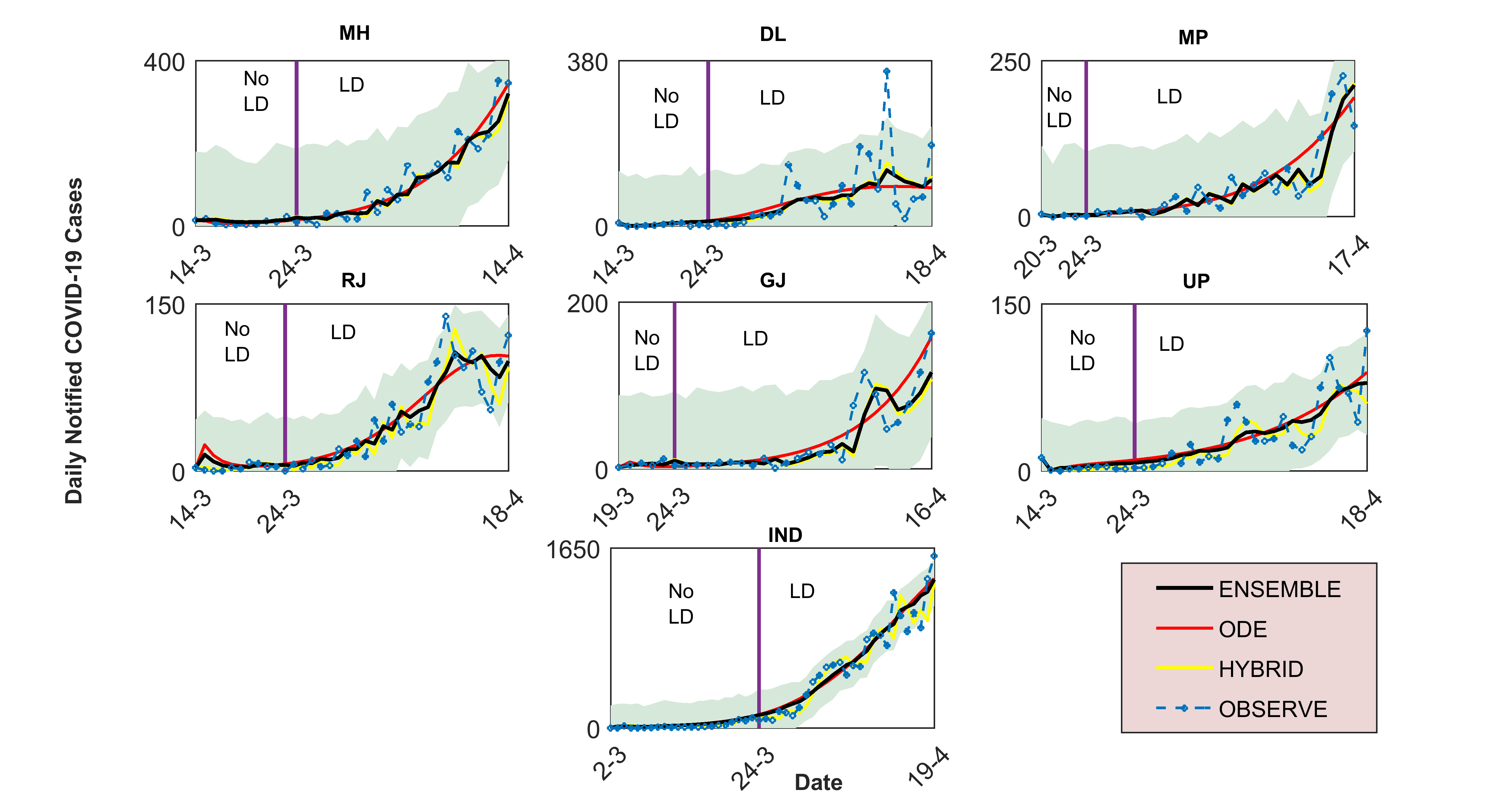
Figure 2: Combination of mechanistic ODE models (Fig 1 and supplementary), Hybrid statistical model, and Ensemble model (0.1) fitting to the daily notified COVID-19 cases form six different states and overall India. Respective subscripts are MH: Maharashtra, DL: Delhi, MP: Madhya Pradesh, RJ: Rajasthan, GJ: Gujarat, UP: Uttar Pradesh, and IND: India. Here, LD indicate the period after the lockdown implementation in overall India started at 25/03/2020 and No LD specifies the period before lockdown. Lockdown effect is considered only for the mechanistic ODE model (Fig 1 and supplementary) and consequently in the ensemble model (0.1). Shaded area specifies the 95% confidence region.

Testing of the three models (the mechanistic ODE model, the hybrid statistical model, and the ensemble model) on daily notified COVID-19 cases from Maharashtra (MH), Delhi (DL), Madhya Pradesh (MP), Rajasthan (RJ), Gujarat (GJ), Uttar Pradesh (UP), and India (IND) are presented in Fig. 2. Based on the performance on testing data from the mentioned seven locations, we estimated the weights ($w_{1}$ and $w_{2}$) for our ensemble model (0.1) (see Table S2 in supplementary). Our result suggest that the mechanistic ODE model (see Fig 1 and supplementary) displayed a better performance in RJ, UP, and IND compared to the hybrid statistical model (see Table S2 in supplementary). For rest of the locations (MH, DL, MP, and GJ), the hybrid statistical model has performed better than the mechanistic ODE model in terms of capturing the trend of the time-series data (Table S2 and Table S3 in supplementary). The ensemble model (0.1), which is derived from a combination of the mechanistic ODE (see Fig 1 and supplementary) and the hybrid statistical model respectively, has provided a robust result in all of these mentioned seven locations in terms of capturing time-series data trend (see Fig. 2).

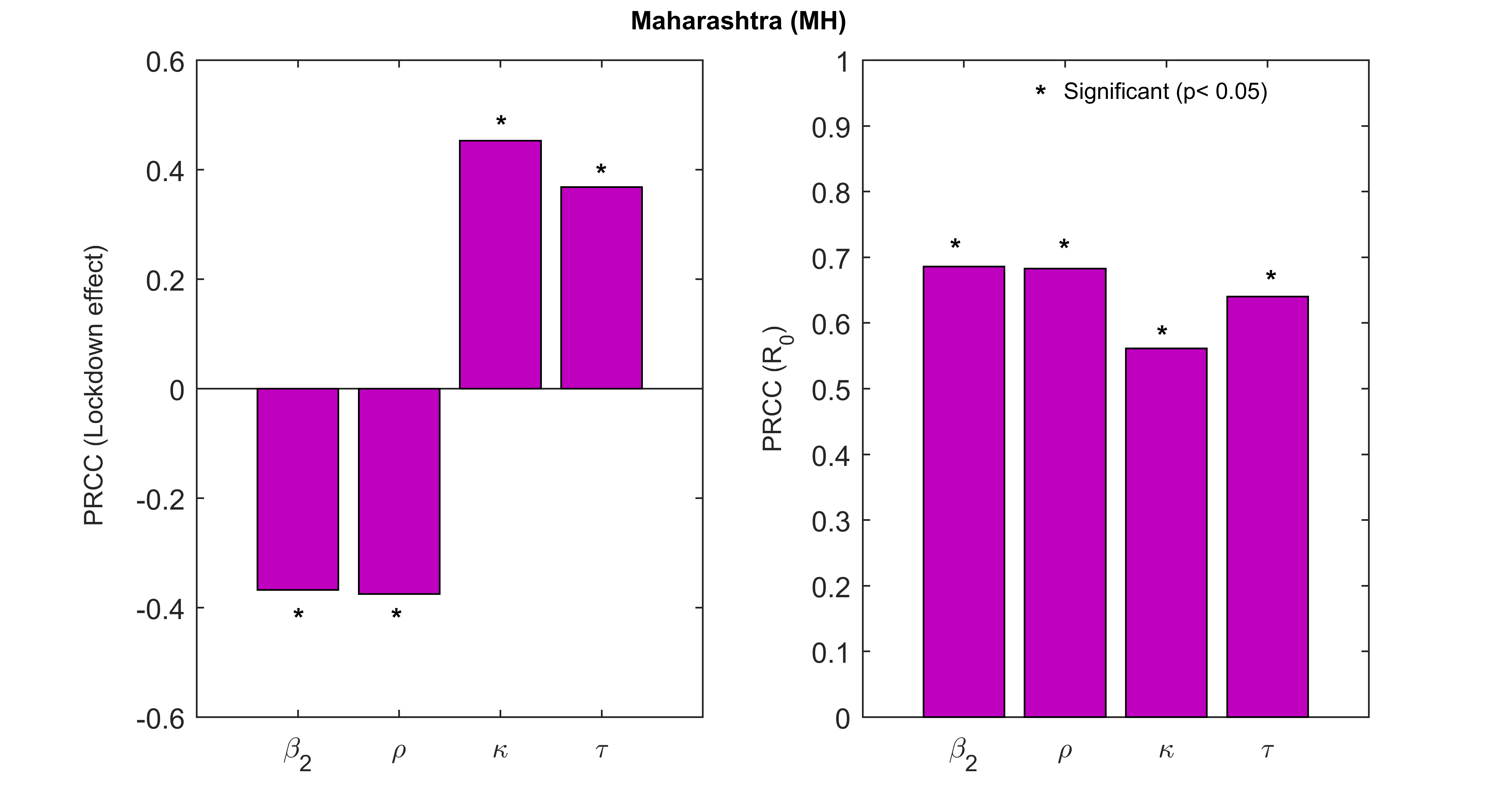
Figure S7: Effect of uncertainty of four epidemiologically measurable and controllable parameters of the mechanistic ODE model (see Table 1 and Fig 1 in the main text) on the effect of lockdown and the basic reproduction number ($R_{0}$). Lockdown effect is measured in terms of the differences in total number of COVID-19 cases occurred during May 3, 2020 till May 20, 2020 in Maharashtra under the lockdown scenarios (A1) and (A5), respectively (see main text). Effect of Uncertainty of these four parameters on the two mentioned responses are measured using Partial Rank Correlation Coefficients (PRCC). $500$ samples for each parameters were drawn using Latin hypercube sampling techniques (LHS) from their respective ranges provided in Table 1 (main text).

The estimates of uninformative parameters of the mechanistic ODE model (Fig 1 and supplementary) suggests that currently in the seven locations (MH, DL, MP, RJ, GJ, UP, and IND) the community infection is mainly dominated by contribution from the asymptomatic infected population (Table 2). Among the seven locations, the lowest percentage of symptomatic infection in the community is found in RJ (about 0.1%) and the highest percentage is found in IND (about 35%) (Table 2). Our estimates suggest that currently in the seven locations (MH, DL, MP, RJ, GJ, UP, and IND), the notification & hospitalization rate of symptomatic infected population is about 0.2% to 23 % (Table 2). Therefore, most of the COVID-19 infections in those mentioned seven locations are currently undetected. Our result agrees with the recent report by the Indian Council of Medical Research (ICMR) Indiatodayasymptomatic . Our estimates of the lockdown rate for MH, DL, MP, RJ, GJ, UP, and IND, respectively, suggest that lockdown is properly implemented in the two metro cities DL and MH. Also, in overall India (IND) lockdown is properly implemented. In these three locations (MH, DL, and IND), about 61% to 77% of the total susceptible population may be successfully home quarantined during the present lockdown period (Table 2). However, for rest of the locations, our results suggest that lockdown may not be successful as about 11% to 49% of the total susceptible population may be isolated (home quarantined) during the current lockdown period in MP, RJ, GJ, and UP, respectively (Table 2). In the seven locations, we found that about 1% to 9% of the total susceptible populations may be exposed to hospital (notified & hospitalized population) related contacts (Table 2). Considering the fact that estimates of the average hospital-based transmission rates for the seven locations (MH, DL, MP, RJ, GJ, UP, and IND) are very high (Table 2), therefore, may be a significant amount of COVID-19 infection in these seven locations are currently occurring due to notified & hospitalized infected related contacts. These findings can be further justified by analyzing the estimates of the basic ($R_{0}$), the community ($R_{C}$) and the hospitalized ($R_{H}$) reproduction numbers for MH, DL, MP, RJ, GJ, UP, and IND, respectively (see Table 3). Except for the RJ, in the remaining six locations, we found that about 1% to 16% of the total COVID-19 transmission currently occurring from notified & hospitalized infected related contacts (see Table 3). These figures can be increased up to 43% to 69% if proper measures are not taken in MH, DL, MP, GJ, UP, and IND, respectively, (see Table 3). This is a worrisome situation as higher value of the hospital-based transmission rate in MH, DL, MP, GJ, UP, and IND, respectively (Table 2), indicate that there may be super-spreading incidents occurring from hospital-based contacts. In RJ, low contribution of $R_{H}$ on $R_{0}$ (see Table 3) may be due to existence of low percentage of the symptomatic infected population in the community (Table 2) and that leads to low percentage of notified & hospitalized COVID-19 cases. For further investigation on super-spreading events, we carried a global uncertainty and sensitivity analysis of some epidemiologically measurable and controllable parameters from our mechanistic ODE model (Fig 1 and supplementary) namely, $\boldsymbol{\beta_{2}}$: average rate of transmission occurring from notified & hospitalized based contact (it can be controllable following the WHO guidelines WHOhospitaltransmission ), $\boldsymbol{\rho}$: fraction of susceptible population that are exposed to hospital-based contact (it can be reduced by following proper guidelines from the WHO WHOhospitaltransmission ), $\boldsymbol{\kappa}$: fraction of the newly infected that are symptomatic (Rapid COVID-19 testing can provide an accurate estimate), $\boldsymbol{\tau}$: hospitalization & notification rate of symptomatic infected population (it also depend on number of COVID-19 testing) on the basic reproduction number ($R_{0}$). Partial rank correlation coefficients (PRCC) and its corresponding $p$-value suggested that all these four parameters have significant positive correlation with $R_{0}$ (see Fig. 4 and Fig. S7 to Fig.S12 in supplementary). Furthermore, high positive correlation of $\rho$ on $R_{0}$ indicate that small increase in the percentage of susceptible population from the community that are exposed hospital-based transmission will leads to significant increase in COVID-19 force of infection. Considering the fact that estimated value of $\beta_{2}$ (see Table 2) in MH, DL, MP, RJ, GJ, UP, and IND, respectively are very high (much higher than community transmission rate), therefore, a small increase in $\rho$ may leads to a larger COVID-19 outbreak in those seven locations. Therefore, until and otherwise any preventive measures are taken in these locations, a larger COVID-19 outbreak may trigger from hospitals and quarantine centers.

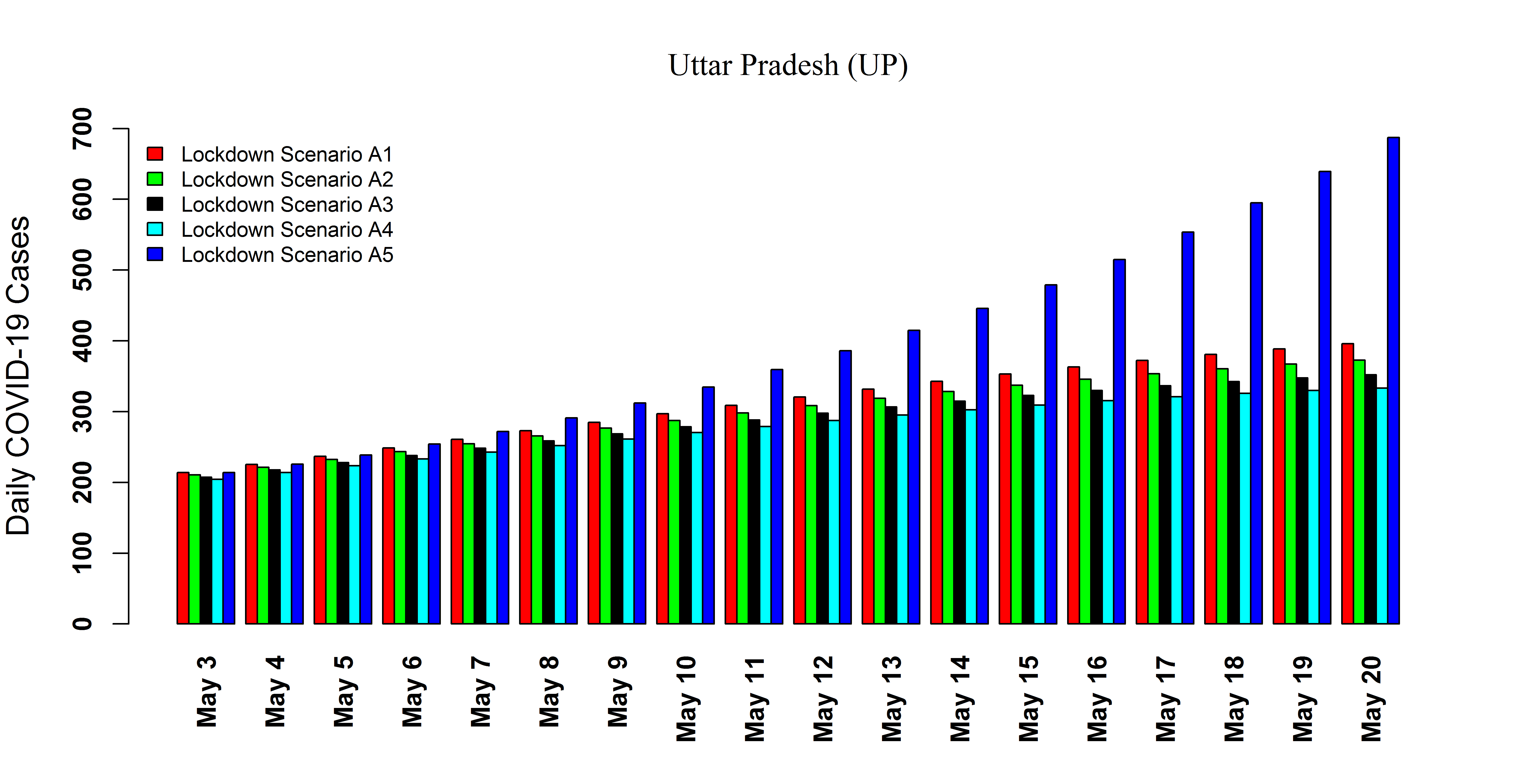
Figure S6: Ensemble model (see main text) forecast for the daily notified COVID-19 cases in Uttar Pradesh during May 3, 2020 till May 20, 2020 under five different lockdown scenarios. Lockdown Scenarios (A1) and (A5) are same as Figure S1. However, under lockdown scenarios (A2) to (A4), projections are made with 10%, 20% and 30% increment in the current estimate of the lockdown rate, respectively (see Table 2 in main text).

Using the ensemble model (0.1), we forecast daily as well as total COVID-19 cases under five different lockdown scenarios in MH, DL, MP, RJ, GJ, UP, and IND, respectively, from May 3, 2020 to May 20, 2020, (see Fig. 3, Table 4 and Fig. S1 to Fig. S6 in supplementary). Comparing the projected total COVID-19 cases during May 3, 2020 to May 20, 2020, (see Table 4) with the total observed cases indiacovid2020track during March 2, 2020 till April 29, 2020, we found about two fold increase in the total cases in MH, MP, GJ, UP, and IND, respectively. In summary, our forecast result suggest that in the coming two weeks a significant increase in cases may be observed in most of these locations.

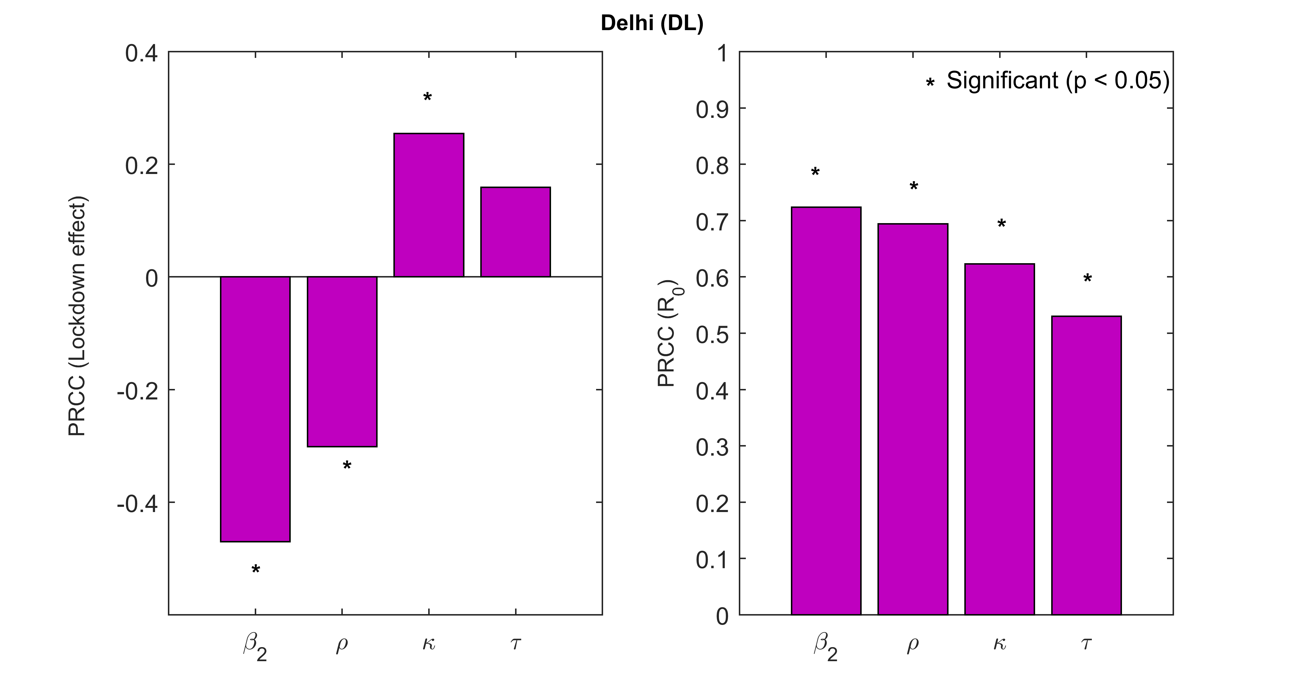
Figure S8: Effect of uncertainty of four epidemiologically measurable and controllable parameters of the mechanistic ODE model (see Table 1 and Fig 1 in the main text) on the effect of lockdown and the basic reproduction number ($R_{0}$). Lockdown effect is measured in terms of the differences in total number of COVID-19 cases occurred during May 3, 2020 till May 20, 2020 in Delhi under the lockdown scenarios (A1) and (A5), respectively (see main text). Effect of Uncertainty of these four parameters on the two mentioned responses are measured using Partial Rank Correlation Coefficients (PRCC). $500$ samples for each parameters were drawn using Latin hypercube sampling techniques (LHS) from their respective ranges provided in Table 1 (main text).

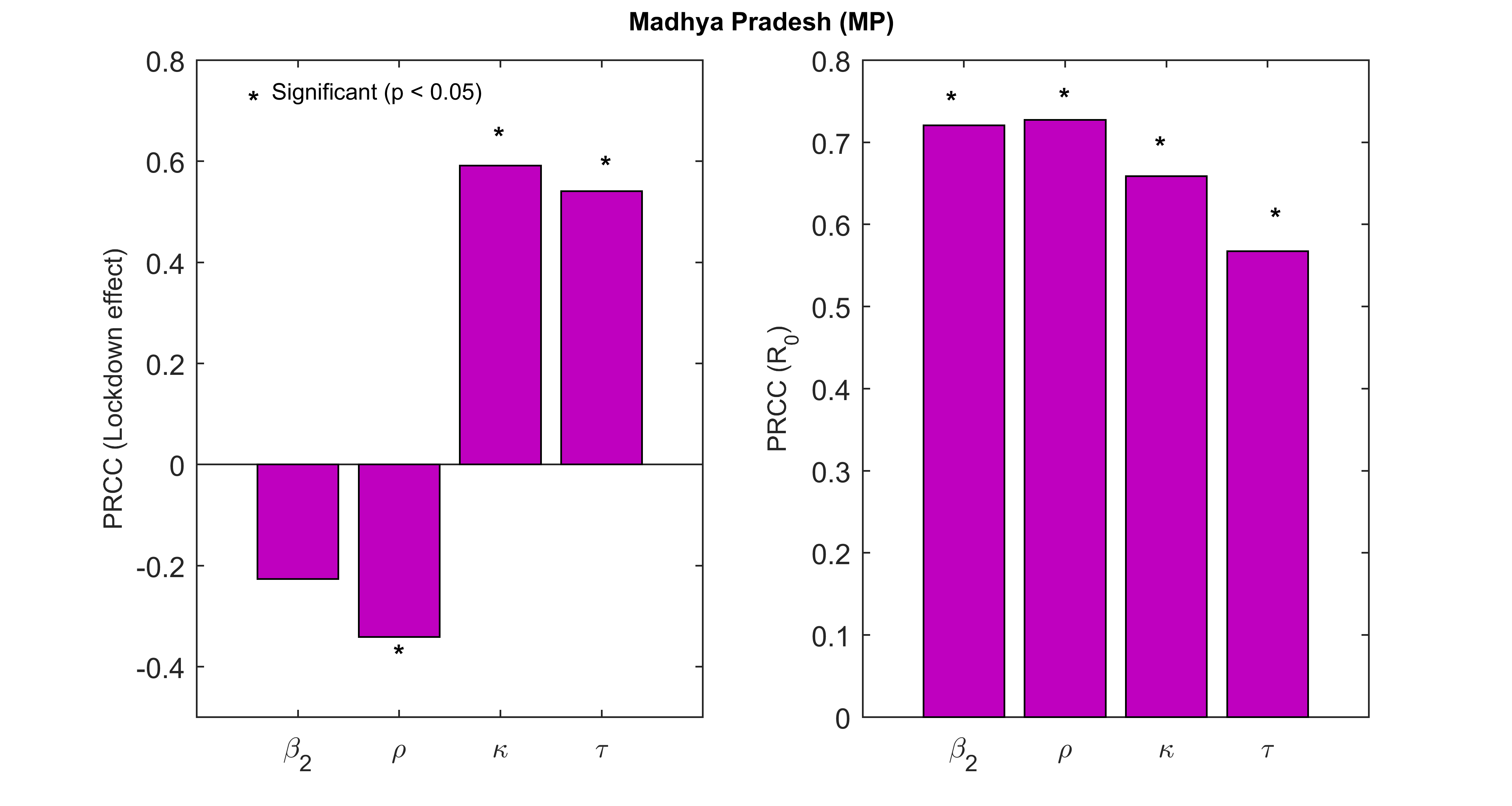
Figure S9: Effect of uncertainty of four epidemiologically measurable and controllable parameters of the mechanistic ODE model (see Table 1 and Fig 1 in the main text) on the effect of lockdown and the basic reproduction number ($R_{0}$). Lockdown effect is measured in terms of the differences in total number of COVID-19 cases occurred during May 3, 2020 till May 20, 2020 in Madhya Pradesh under the lockdown scenarios (A1) and (A5), respectively (see main text). Effect of Uncertainty of these four parameters on the two mentioned responses are measured using Partial Rank Correlation Coefficients (PRCC). $500$ samples for each parameters were drawn using Latin hypercube sampling techniques (LHS) from their respective ranges provided in Table 1 (main text).

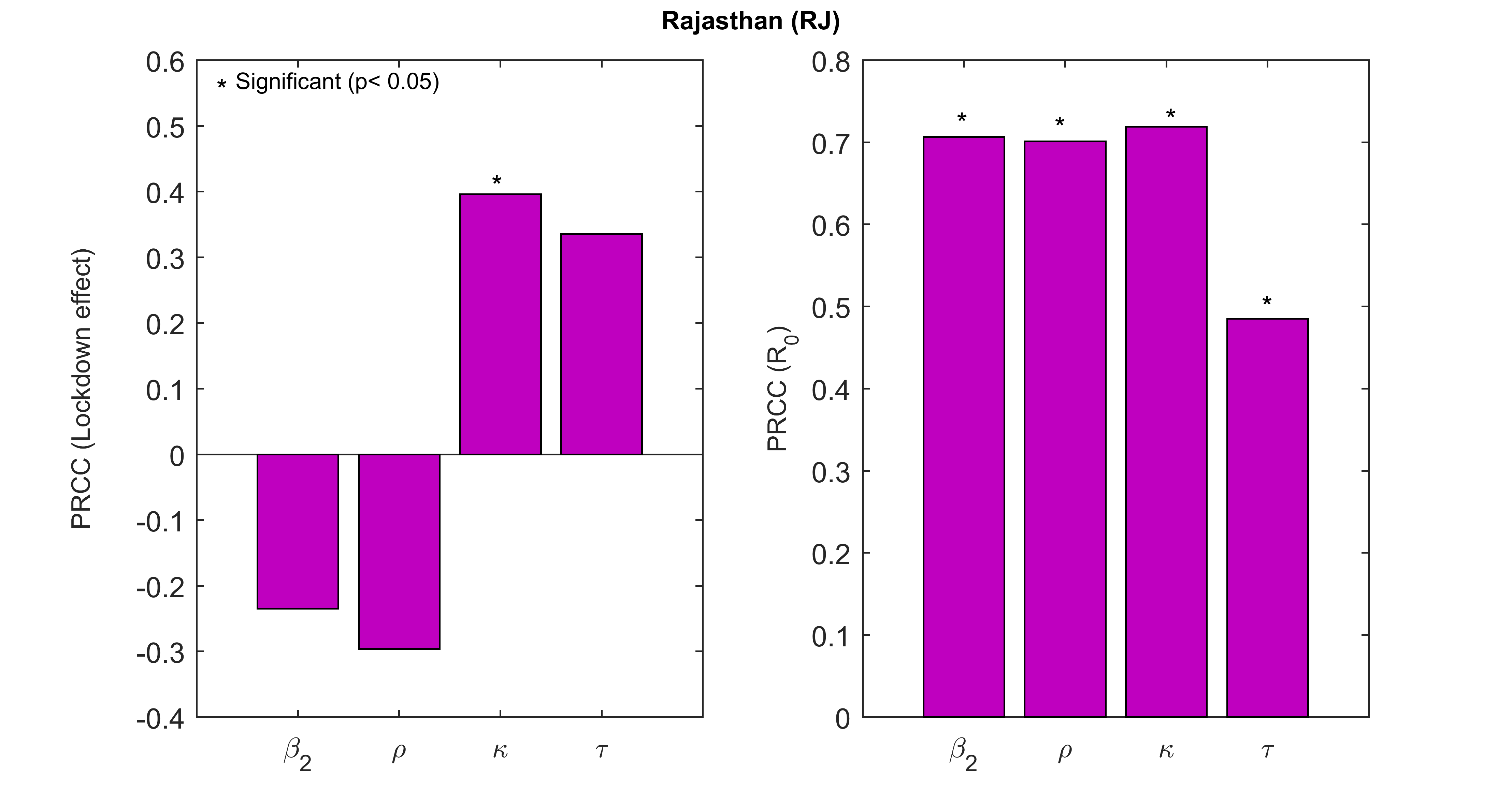
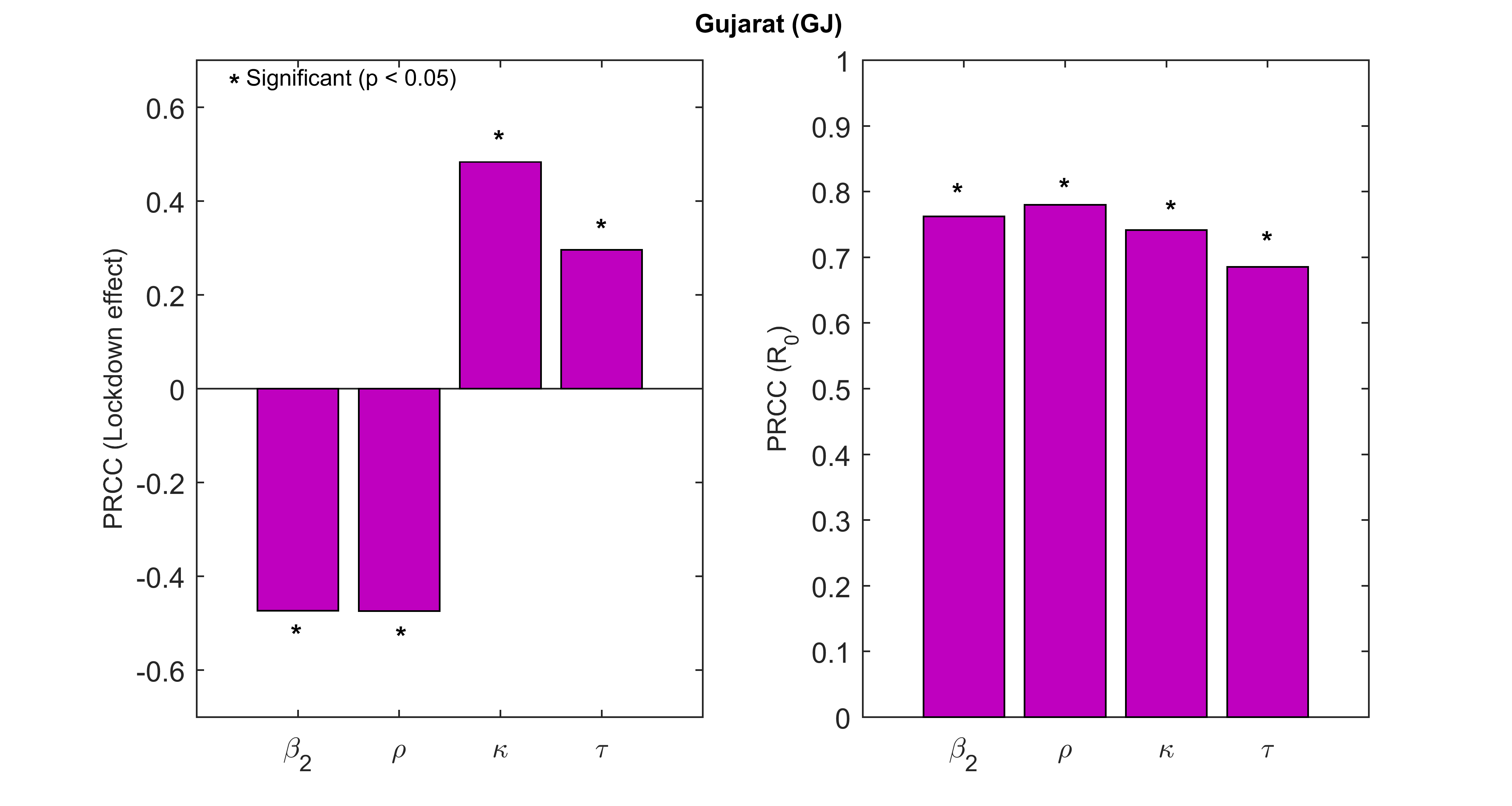
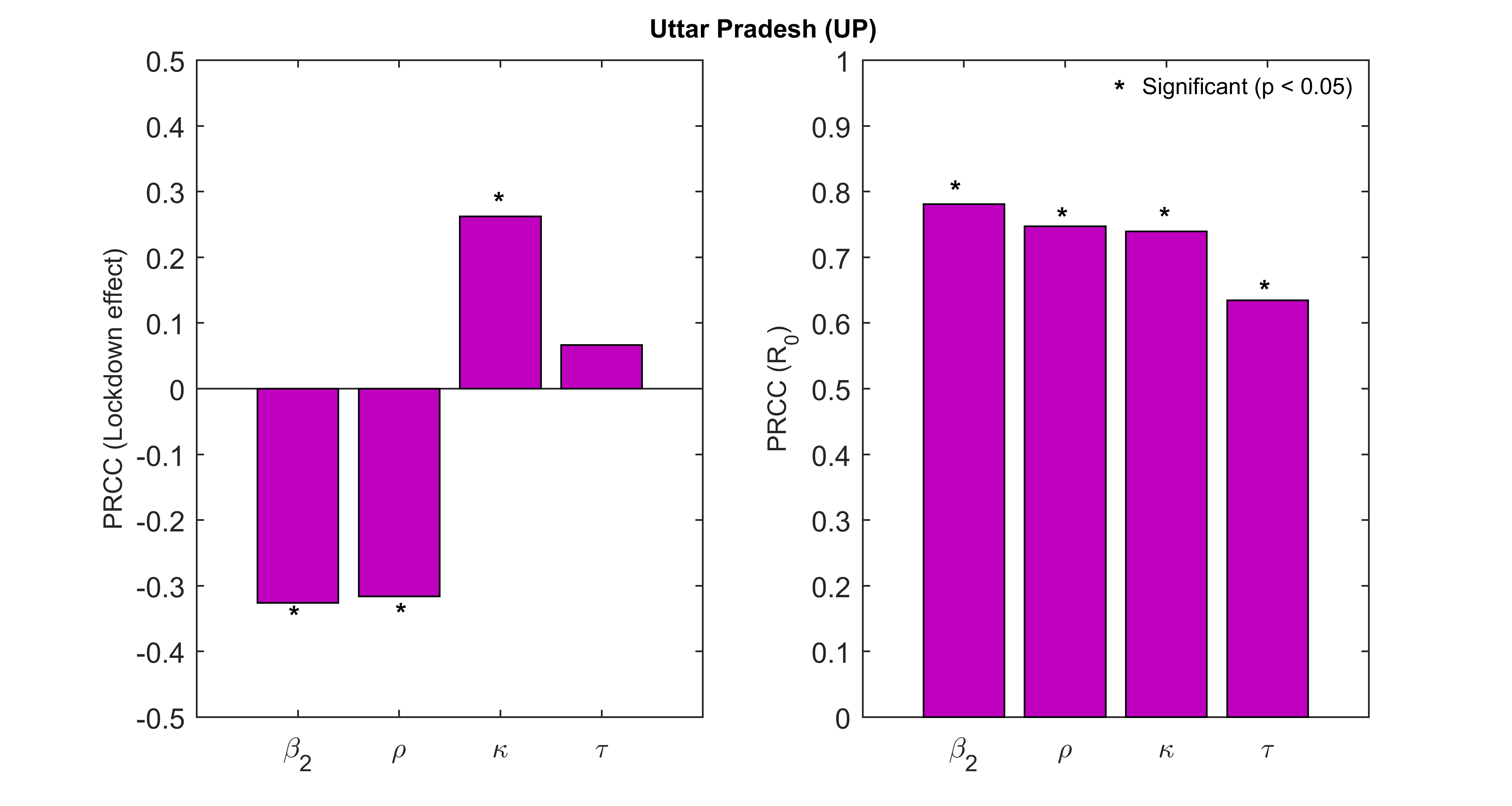
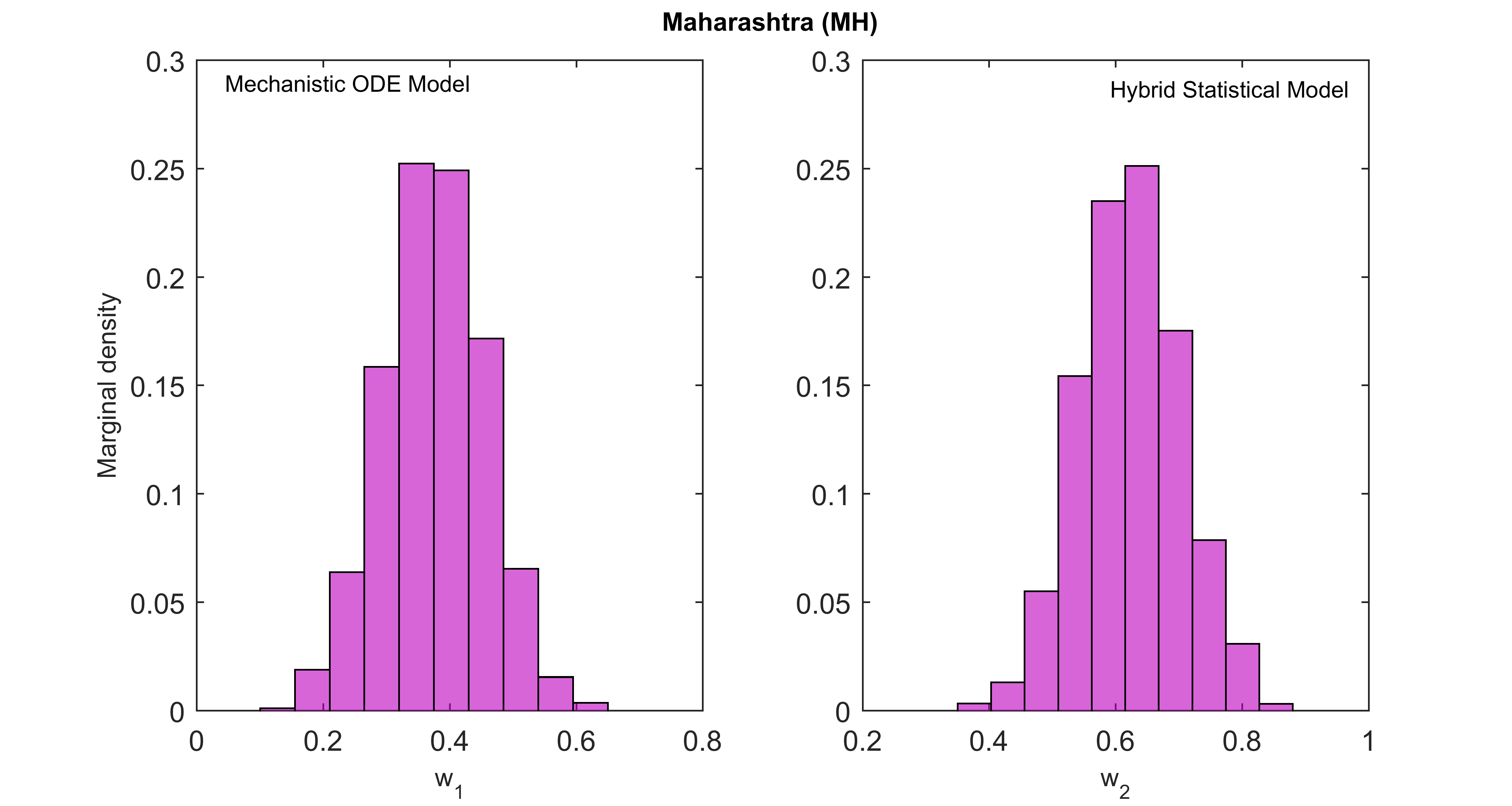
Figure S10: Effect of uncertainty of four epidemiologically measurable and controllable parameters of the mechanistic ODE model (see Table 1 and Fig 1 in the main text) on the effect of lockdown and the basic reproduction number ($R_{0}$). Lockdown effect is measured in terms of the differences in total number of COVID-19 cases occurred during May 3, 2020 till May 20, 2020 in Rajasthan under the lockdown scenarios (A1) and (A5), respectively (see main text). Effect of Uncertainty of these four parameters on the two mentioned responses are measured using Partial Rank Correlation Coefficients (PRCC). $500$ samples for each parameters were drawn using Latin hypercube sampling techniques (LHS) from their respective ranges provided in Table 1 (main text).

To determine which epidemiologically measurable and controllable parameters are most influencing the effect of lockdown, we carried out a global uncertainty analysis of $\beta_{2}$, $\rho$, $\kappa$, and $\tau$ on the lockdown effect. The lockdown effect is measured in terms of differences in the total number of COVID-19 cases during May 3, 2020 till May 20, 2020, in MH, DL, MP, RJ, GJ, UP, and IND, respectively, under the lockdown scenarios (A1) and (A5), respectively (see method section for details). For MH, PRCC and its corresponding $p$-value suggested that all these four parameters have significant influence on the lockdown effect (see Fig. S7 in supplementary). Furthermore, significant negative correlation of $\beta_{2}$, and $\rho$ with the lockdown effect (see Fig. S7 in supplementary) suggested that only home quarantined the community may not be sufficient to reduce COVID-19 transmission in MH. Govt. and the policy makers may also have to focus on reducing the transmission occurring from hospital premises based on the guidelines from the WHO WHOhospitaltransmission . For DL, PRCC and its corresponding $p$-value suggested that $\beta_{2}$, $\rho$, and $\kappa$ are the main parameters that are influencing the lockdown effect (see Fig. S8 in supplementary). Moreover, significant negative correlation of $\beta_{2}$ and $\rho$ with the lockdown effect and as well as significant positive correlation of $\kappa$ with the lockdown effect (see Fig. S8 in supplementary) implies that an effective lockdown policy in DL may be a combination of lockdown in the community, contact tracing of COVID-19 cases, and with some effort in reducing hospital-based transmission following WHO guidelines WHOhospitaltransmission . For MP, PRCC and its corresponding $p$-value suggested that $\kappa$ and $\tau$ have high positive correlation with the lockdown effect (see Fig. S9 in supplementary). Furthermore, $\rho$ have significant negative correlation with the lockdown effect (see Fig. S9 in supplementary). Therefore an effective lockdown policy in MP may be a strict implementation of lockdown in the red and orange zones, rapid COVID-19 testing in the community and reducing hospital-based transmission by following guidelines from WHO WHOhospitaltransmission . For RJ, PRCC and its corresponding $p$-value suggested that only $\kappa$ have significant positive correlation with the lockdown effect (see Fig. S10 in supplementary). No significant correlation with hospital-based parameters may be due to existence of low percentage of the symptomatic infected population in the community (see Table 2) and that leads to low percentage of notified & hospitalized based COVID-19 transmission. Therefore, RJ Govt. may focused more on contact tracing in the community with relaxation may be given in the Green and Orange zones to increase the percentage of symptomatic infected in the community. For GJ, PRCC and its corresponding $p$-value suggested that all these four parameters have significant influence on the lockdown effect (see Fig. S11 in supplementary). Furthermore, significant negative correlation of $\beta_{2}$, and $\rho$ with the lockdown effect (see Fig. S11 in supplementary) indicate that only home quarantined the community may not be sufficient to reduce COVID-19 transmission in GJ. Govt. of GJ and policy makers may also have to focus on reducing the transmission occurring from hospital premises based on the guidelines from the WHO WHOhospitaltransmission . For UP, PRCC and its corresponding $p$-value suggested that $\beta_{2}$, $\rho$, and $\kappa$ are the main parameters that are influencing the lockdown effect (see Fig. S12 in supplementary). Moreover, significant negative correlation of $\beta_{2}$ and $\rho$ with the lockdown effect and as well as significant positive correlation of $\kappa$ with the lockdown effect (see Fig. S12 in supplementary) implies that an effective lockdown policy in UP may be a combination of lockdown (relaxation in Green zone), contact tracing in community with effort in reducing hospital-based transmission following the WHO guidelines WHOhospitaltransmission . Finally for IND, PRCC and its corresponding $p$-value suggested that $\beta_{2}$ and $\rho$ are the main parameters that are most influencing the lockdown effect (see Fig. 4). Therefore, only home quarantined the community may not be sufficient to reduce COVID-19 transmission in IND. Govt. of IND and the policy makers may also have to focus on reducing the transmission occurring from hospital premises based on the guidelines from the WHO WHOhospitaltransmission .

Conclusion

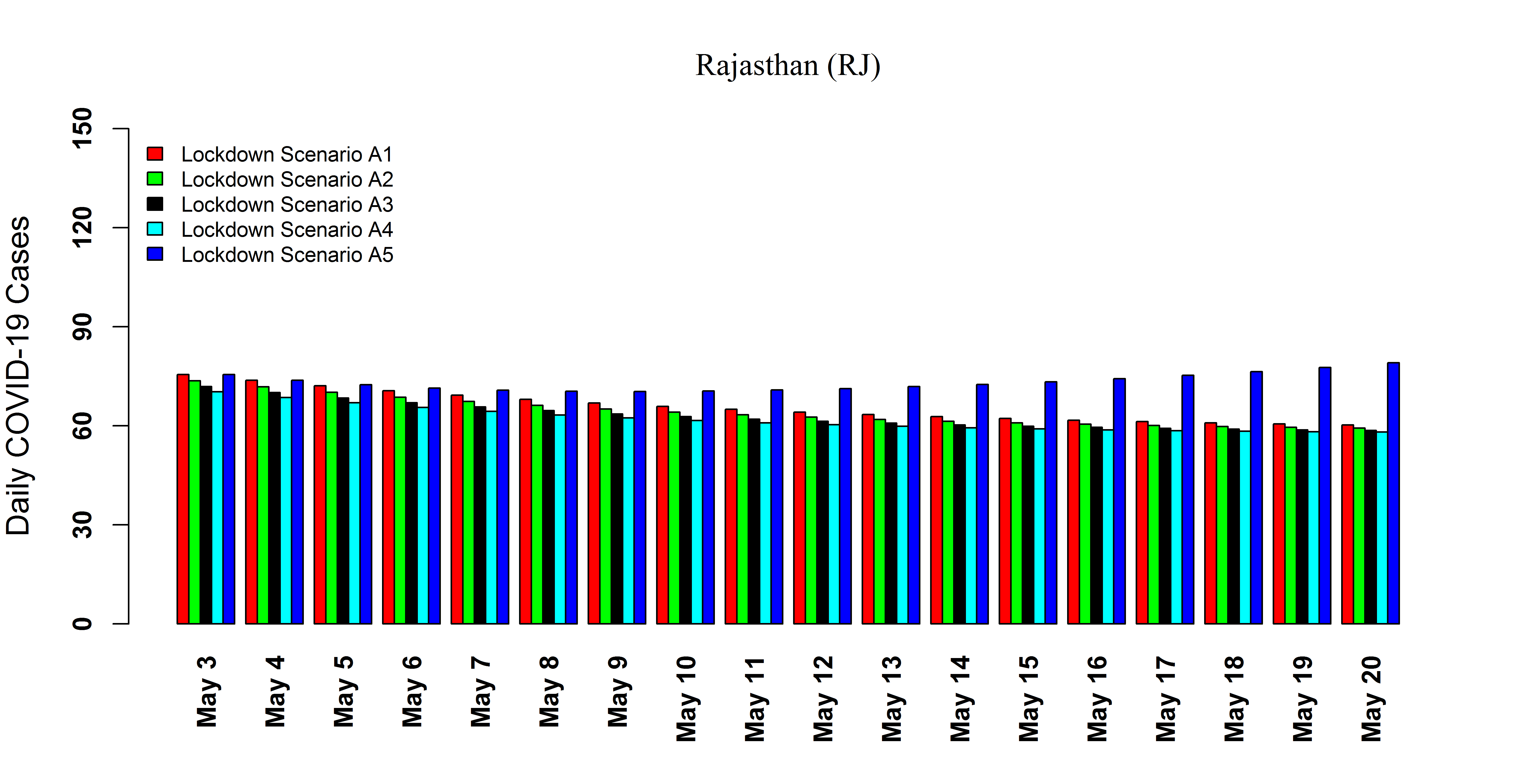
Figure S4: Ensemble model (see main text) forecast for the daily notified COVID-19 cases in Rajasthan during May 3, 2020 till May 20, 2020 under five different lockdown scenarios. Lockdown Scenarios (A1) and (A5) are same as Figure S1. However, under lockdown scenarios (A2) to (A4), projections are made with 10%, 20% and 30% increment in the current estimate of the lockdown rate, respectively (see Table 2 in main text).

Our analysis of the mechanistic model with hospital-based COVID-19 transmission suggest that most of the new infections occurring in India as well most of the states are currently undetected. Furthermore, a global sensitivity analysis of two epidemiologically controllable parameters from the hospital-based transmission on the basic reproduction nuber ($R_{0}$), indicate that if appropriate preventive measures are not taken immediately, a much larger COVID-19 outbreak may trigger due to the transmission occurring from the hospitalized & notified based contacts. Moreover, our ensemble forecast model (0.1) predicted a substantial percentage of increase in the COVID-19 notified cases during May 3, 2020 till May 20, 2020, (see Table 4) in most of these locations. In Rajasthan, trend of the forecast data (see Fig S4 in supplementary) during May 3, 2020 till May 20, 2020, is showing a decreasing trend. This is may be due to low number of hospitalized and reported cases in this state (see Table 2). However, cases may rise in Rajasthan if relaxation in lockdown is applied. Furthermore, trend of the forecast data in overall India (see Fig 3) during May 3, 2020 till May 20, 2020, indicating the fact that reaching the peak of the COVID-19 epidemic curve may be a long way ahead for India. Finally, based on our results of global sensitivity analysis of the four important epidemiologically measurable & controllable parameters on the lockdown effect, we are suggesting the following policy that may reduce the threat of a larger COVID-19 outbreak in the coming days:

Effective Lockdown Policy: Dividing different states into three clusters (red, orange, and green) is well appreciated as it increases the percentage of symptomatic infection in the community. However, more COVID-19 testing is needed as it increases the number of notified & hospitalized cases over the states. It is much easier to reduce hospital-based transmission in compare to community transmission. To reduce the hospitalized & notified based contacts, an efficient disaster management team is required. They will continuously monitor the situations in different hospitals and quarantine centers across India. This team must ensure that proper safety measures are being followed based on the guidelines provided by ICMR and WHO WHOhospitaltransmission .

Conflict of interests

The authors declare that they have no conflicts of interest.

Figures

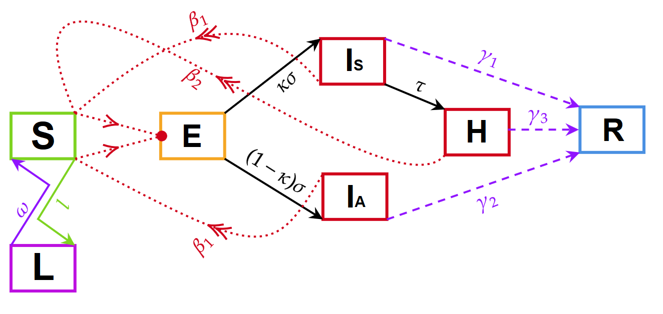
Figure 1: A Flow diagram of the mechanistic ODE model with hospital-based COVID-19 transmission and lockdown effect. Different class of population shown in this figure are $S$: Susceptible population, $E$: Exposed population, $I_{S}$: COVID-19 symptomatic infected population, $I_{A}$: COVID-19 asymptomatic infected population, $H$: Notified & Hospital individuals suffering from COVID-19 infection, $R$: COVID-19 recovered population, and $L$: Home quarantined susceptible population during lockdown, respectively. Epidemiological information of the parameters shown in this figure are provided in Table 1.

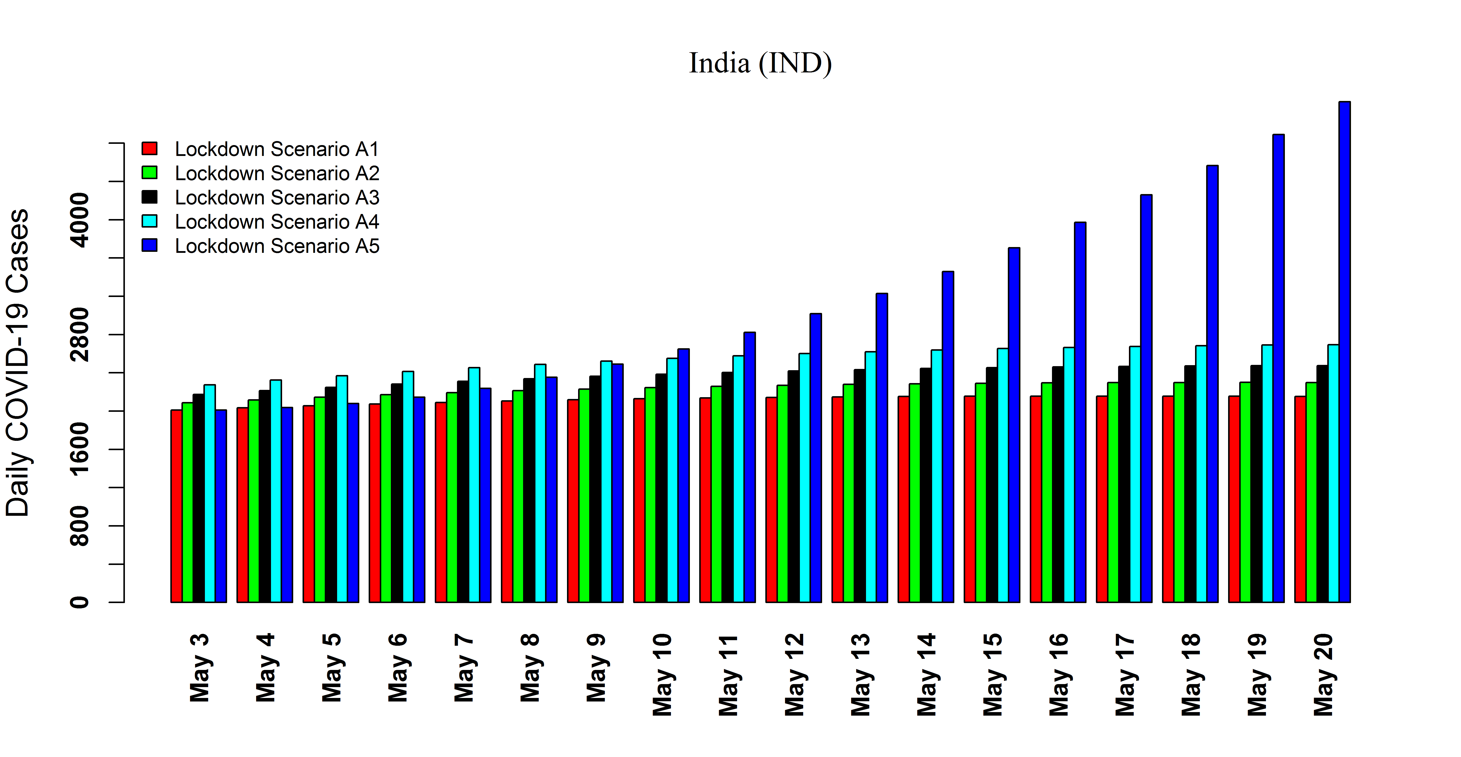
Figure 3: Ensemble model (0.1) forecast for the daily notified COVID-19 cases in India during May 3, 2020 till May 20, 2020 under five different lockdown scenarios. Under lockdown scenarios (A2) to (A4), projections are made with 10%, 20% and 30% decrement in the current estimate of the lockdown rate, respectively (see Table 2). In lockdown scenario (A1), projections are made with current estimated lockdown rate (see Table 2). Finally, in the lockdown scenario (A5), projections are made with no lockdown during May 3, 2020 till May 20, 2020.

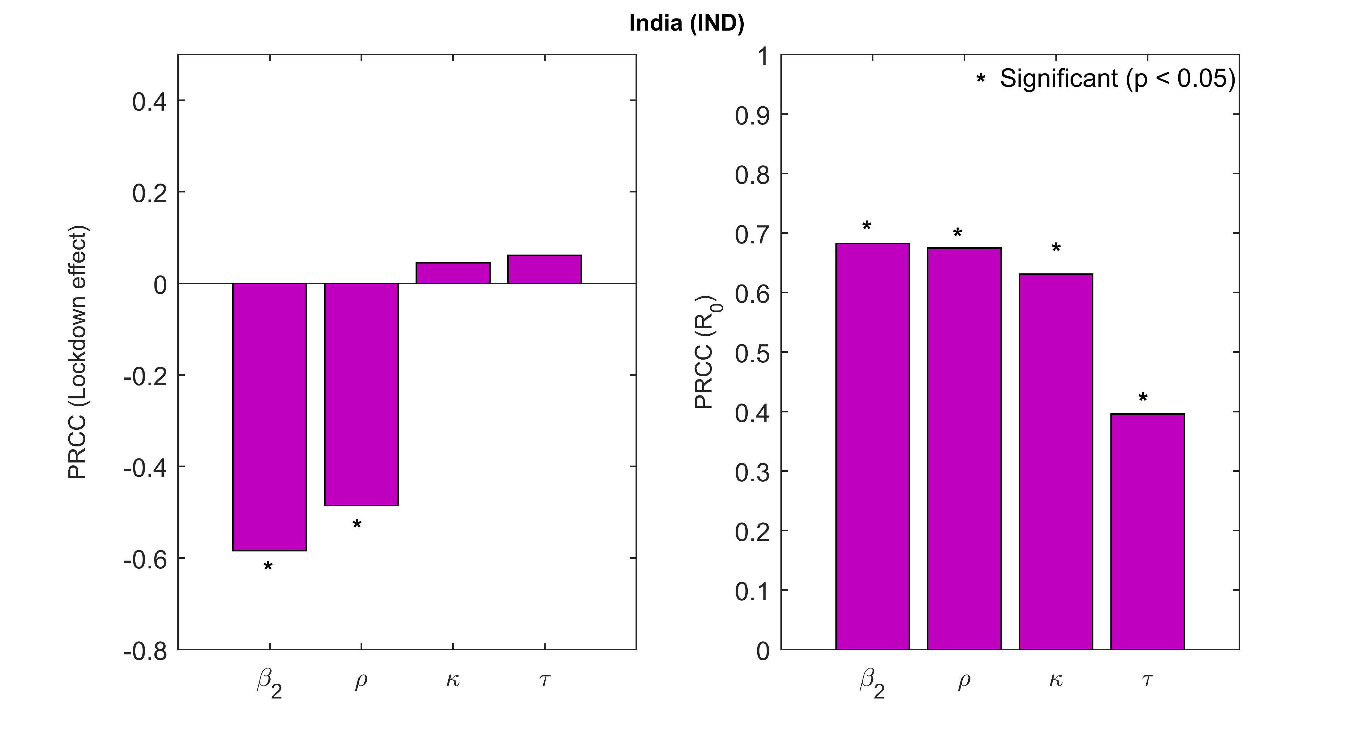
Figure 4: Effect of uncertainty of four epidemiologically measurable and controllable parameters of the mechanistic ODE model (see Fig 1, Table 1 and method section) on the effect of lockdown and the basic reproduction number ($R_{0}$). Lockdown effect is measured in terms of the differences in total number of COVID-19 cases occurred during May 3, 2020 till May 20, 2020 in India under the lockdown scenarios (A1) and (A5), respectively (see method section). Effect of Uncertainty of these four parameters on the two mentioned responses are measured using Partial Rank Correlation Coefficients (PRCC). $500$ samples for each parameters were drawn using Latin hypercube sampling techniques (LHS) from their respective ranges provided in Table 1.

Tables

Table 1: Parameters with their respective epidemiological information for the mechanistic ODE model (see Fig 1 and supplementary) for COVID-19.

Parameters	Biological Meaning	Value/Ranges	Reference
$\Pi$ $=$ $\mu$ $\times$ $N(0)$	Recruitment rate of human population	Differs over states	-
$\displaystyle\frac{1}{\mu}$	Average life expectancy at birth	Differs over states	nitiaayog20
$\displaystyle\beta_{1}$	Average transmission rate of a symptomatic and asymptomatic COVID-19 infected	(0 - 500) $day^{-1}$	Estimated
$\displaystyle\beta_{2}$	Average transmission rate of a notified & hospitalized COVID-19 infected	(0 - 500) $day^{-1}$	Estimated
$\displaystyle\rho$	Fraction of the susceptible population that are exposed to hospital-based transmission	0 - 0.2	Estimated
$\displaystyle\frac{1}{\sigma}$	COVID-19 incubation period	(1 - 14) days	Estimated
$\displaystyle\kappa$	Fraction of the COVID-19 exposed population that become symptomatic infected	0 - 1	Estimated
$\displaystyle\gamma_{1}$	Average recovery rate of symptomatic infection	($\displaystyle\gamma_{3}$ - 1) $day^{-1}$	Estimated
$\displaystyle\gamma_{2}$	Average recovery rate of asymptomatic infection	($\displaystyle\gamma_{3}$ - 1) $day^{-1}$	Estimated
$\displaystyle\tau$	Average hospitalization rate for the COVID-19 symptomatic individuals	(0 - 1) $day^{-1}$	Estimated
$\displaystyle\delta$	Average death rate due to COVID-19 infection in hospital	Differs over states	indiacovid2020track
$\displaystyle\gamma_{3}$	Average recovery rate of the notified & hospitalized populations	Differs over states	indiacovid2020track
$\displaystyle l$	Average lockdown rate	(0 - 0.9) $day^{-1}$	Estimated
$\displaystyle\frac{1}{\omega}$	Current lockdown period in India	40 days	timesofindia20b ; financialexpress20

Table 2: Estimated uninformative parameters of the mechanistic ODE model combinations  (see Fig 1 and supplementary). Respective subscripts are MH: Maharashtra, DL: Delhi, MP: Madhya Pradesh, RJ: Rajasthan, GJ: Gujarat, UP: Uttar Pradesh, and IND: India. All data are given in the format Estimate (95% CI).

Region	$\boldsymbol{\beta_{1}}$	$\boldsymbol{\beta_{2}}$	$\boldsymbol{\rho}$ $\times$ $100$	$\boldsymbol{\sigma}$	$\boldsymbol{\kappa}$	$\boldsymbol{\gamma_{1}}$	$\boldsymbol{\tau\times 100}$	$\boldsymbol{\gamma_{2}}$	$\boldsymbol{l}\times 100$
MH	$\begin{subarray}{c}2.03\\ \\ (1.05-2.75)\end{subarray}$	$\begin{subarray}{c}21.6\\ \\ (2.6-54.7)\end{subarray}$	$\begin{subarray}{c}7.98\\ \\ (0.24-9.78)\end{subarray}$	$\begin{subarray}{c}0.163\\ \\ (0.073-0.196)\end{subarray}$	$\begin{subarray}{c}0.118\\ \\ (0.03-0.165)\end{subarray}$	$\begin{subarray}{c}0.963\\ \\ (0.144-0.974)\end{subarray}$	$\begin{subarray}{c}5.05\\ \\ (2.76-85.3)\end{subarray}$	$\begin{subarray}{c}0.863\\ \\ (0.341-0.991)\end{subarray}$	$\begin{subarray}{c}61.5\\ \\ (2.51-97.3)\end{subarray}$
DL	$\begin{subarray}{c}1.83\\ \\ (0.557-3.54)\end{subarray}$	$\begin{subarray}{c}220.2\\ \\ (12.97-488.8)\end{subarray}$	$\begin{subarray}{c}7.66\\ \\ (0.25-9.67)\end{subarray}$	$\begin{subarray}{c}0.211\\ \\ (0.075-0.748)\end{subarray}$	$\begin{subarray}{c}0.039\\ \\ (0.002-0.039)\end{subarray}$	$\begin{subarray}{c}0.96\\ \\ (0.321-0.987)\end{subarray}$	$\begin{subarray}{c}8.5\\ \\ (3.8-96.3)\end{subarray}$	$\begin{subarray}{c}0.764\\ \\ (0.328-0.988)\end{subarray}$	$\begin{subarray}{c}70.8\\ \\ (13.1-87.8)\end{subarray}$
MP	$\begin{subarray}{c}1.45\\ \\ (1.04-2.91)\end{subarray}$	$\begin{subarray}{c}42.1\\ \\ (25.4-486)\end{subarray}$	$\begin{subarray}{c}5.88\\ \\ (0.24-9.72)\end{subarray}$	$\begin{subarray}{c}0.194\\ \\ (0.073-0.242)\end{subarray}$	$\begin{subarray}{c}0.014\\ \\ (0.002-0.098)\end{subarray}$	$\begin{subarray}{c}0.827\\ \\ (0.141-0.980)\end{subarray}$	$\begin{subarray}{c}14\\ \\ (3.52-92.2)\end{subarray}$	$\begin{subarray}{c}0.585\\ \\ (0.21-0.978)\end{subarray}$	$\begin{subarray}{c}34.8\\ \\ (12.7-88.6)\end{subarray}$
RJ	$\begin{subarray}{c}1.16\\ \\ (0.557-2.74)\end{subarray}$	$\begin{subarray}{c}325.6\\ \\ (3.71-484)\end{subarray}$	$\begin{subarray}{c}1.33\\ \\ (0.07-9.56)\end{subarray}$	$\begin{subarray}{c}0.937\\ \\ (0.148-0.949)\end{subarray}$	$\begin{subarray}{c}0.0011\\ \\ (0.001-0.003)\end{subarray}$	$\begin{subarray}{c}0.337\\ \\ (0.253-0.988)\end{subarray}$	$\begin{subarray}{c}23.2\\ \\ (4.66-96.3)\end{subarray}$	$\begin{subarray}{c}0.814\\ \\ (0.244-0.978)\end{subarray}$	$\begin{subarray}{c}21\\ \\ (10.6-81.2)\end{subarray}$
GJ	$\begin{subarray}{c}0.90\\ \\ (0.53-2.10)\end{subarray}$	$\begin{subarray}{c}186.3\\ \\ (9.64-490)\end{subarray}$	$\begin{subarray}{c}2.32\\ \\ (0.21-9.20)\end{subarray}$	$\begin{subarray}{c}0.54\\ \\ (0.101-0.94)\end{subarray}$	$\begin{subarray}{c}0.028\\ \\ (0.01-0.092)\end{subarray}$	$\begin{subarray}{c}0.84\\ \\ (0.15-0.98)\end{subarray}$	$\begin{subarray}{c}14\\ \\ (4.02-76.2)\end{subarray}$	$\begin{subarray}{c}0.52\\ \\ (0.202-0.98)\end{subarray}$	$\begin{subarray}{c}11.4\\ \\ (2.31-32.2)\end{subarray}$
UP	$\begin{subarray}{c}0.53\\ \\ (0.52-1.92)\end{subarray}$	$\begin{subarray}{c}242\\ \\ (8.23-353)\end{subarray}$	$\begin{subarray}{c}4.29\\ \\ (0.1-9.51)\end{subarray}$	$\begin{subarray}{c}0.66\\ \\ (0.078-0.71)\end{subarray}$	$\begin{subarray}{c}0.12\\ \\ (0.077-0.95)\end{subarray}$	$\begin{subarray}{c}0.78\\ \\ (0.19-0.988)\end{subarray}$	$\begin{subarray}{c}2.38\\ \\ (0.2-5)\end{subarray}$	$\begin{subarray}{c}0.408\\ \\ (0.218-0.982)\end{subarray}$	$\begin{subarray}{c}48.9\\ \\ (12.3-87.6)\end{subarray}$
IND	$\begin{subarray}{c}2.25\\ \\ (1.29-3.24)\end{subarray}$	$\begin{subarray}{c}499\\ \\ (494-499.8)\end{subarray}$	$\begin{subarray}{c}8.99\\ \\ (0.32-9.70)\end{subarray}$	$\begin{subarray}{c}0.098\\ \\ (0.072-0.15)\end{subarray}$	$\begin{subarray}{c}0.35\\ \\ (0.07-0.96)\end{subarray}$	$\begin{subarray}{c}0.72\\ \\ (0.38-0.99)\end{subarray}$	$\begin{subarray}{c}0.23\\ \\ (0.03-0.53)\end{subarray}$	$\begin{subarray}{c}0.995\\ \\ (0.25-0.9959)\end{subarray}$	$\begin{subarray}{c}76.6\\ \\ (35.5-89.2)\end{subarray}$

Table 3: Estimates of the basic, the community and the hospital reproduction numbers. The informative and uninformative parameters of the mechanistic ODE model (see Fig 1 and supplementary) during the estimation of the different reproduction numbers are taken from Table 1 and Table 2, respectively. Respective subscripts MH, DL, MP, RJ, GJ, UP, and IND are same as Table 2. All data are given in the format Estimate (95% CI).

Region	$\boldsymbol{R_{0}}$	$\boldsymbol{R_{C}}$	% $\boldsymbol{R_{0}}$	$\boldsymbol{R_{H}}$	% $\boldsymbol{R_{0}}$
MH	$\begin{subarray}{c}2.371\\ \\ (2.095-4.005)\end{subarray}$	$\begin{subarray}{c}2.309\\ \\ (1.542-3.894)\end{subarray}$	$\begin{subarray}{c}97.37\\ \\ (55.46-99.93)\end{subarray}$	$\begin{subarray}{c}0.0623\\ \\ (0.0019-1.254)\end{subarray}$	$\begin{subarray}{c}2.63\\ \\ (0.1-44.54)\end{subarray}$
DL	$\begin{subarray}{c}2.54\\ \\ (1.37-5.52)\end{subarray}$	$\begin{subarray}{c}2.37\\ \\ (0.934-5.49)\end{subarray}$	$\begin{subarray}{c}93.46\\ \\ (56.91-99.95)\end{subarray}$	$\begin{subarray}{c}0.1658\\ \\ (0.0016-0.8236)\end{subarray}$	$\begin{subarray}{c}6.53\\ \\ (0.048-43.09)\end{subarray}$
MP	$\begin{subarray}{c}2.497\\ \\ (2.21-6.11)\end{subarray}$	$\begin{subarray}{c}2.467\\ \\ (1.68-5.63)\end{subarray}$	$\begin{subarray}{c}98.82\\ \\ (49.22-99.81)\end{subarray}$	$\begin{subarray}{c}0.0296\\ \\ (0.0062-2.045)\end{subarray}$	$\begin{subarray}{c}1.18\\ \\ (0.19-50.78)\end{subarray}$
RJ	$\begin{subarray}{c}1.43\\ \\ (1.42-3.78)\end{subarray}$	$\begin{subarray}{c}1.42\\ \\ (1.405-3.76)\end{subarray}$	$\begin{subarray}{c}99.46\\ \\ (94.40-100)\end{subarray}$	$\begin{subarray}{c}0.01\\ \\ (0-0.068)\end{subarray}$	$\begin{subarray}{c}0.54\\ \\ (0-3.66)\end{subarray}$
GJ	$\begin{subarray}{c}1.835\\ \\ (1.51-4.86)\end{subarray}$	$\begin{subarray}{c}1.706\\ \\ (0.895-3.72)\end{subarray}$	$\begin{subarray}{c}93.02\\ \\ (31.4-99.56)\end{subarray}$	$\begin{subarray}{c}0.128\\ \\ (0.0083-2.68)\end{subarray}$	$\begin{subarray}{c}6.98\\ \\ (0.43-68.60)\end{subarray}$
UP	$\begin{subarray}{c}1.46\\ \\ (1.35-3.14)\end{subarray}$	$\begin{subarray}{c}1.22\\ \\ (0.787-2.88)\end{subarray}$	$\begin{subarray}{c}84\\ \\ (39.21-99.96)\end{subarray}$	$\begin{subarray}{c}0.233\\ \\ (0.001-1.47)\end{subarray}$	$\begin{subarray}{c}16\\ \\ (0.039-60.79)\end{subarray}$
IND	$\begin{subarray}{c}2.81\\ \\ (2.15-4.94)\end{subarray}$	$\begin{subarray}{c}2.56\\ \\ (1.92-4.86)\end{subarray}$	$\begin{subarray}{c}91.28\\ \\ (84.63-99.84)\end{subarray}$	$\begin{subarray}{c}0.245\\ \\ (0.0048-0.388)\end{subarray}$	$\begin{subarray}{c}8.72\\ \\ (0.16-15.37)\end{subarray}$

Table 4: Ensemble model (0.1) forecast of the total notified COVID-19 cases during May 3, 2020 till May 20, 2020. Respective subscripts MH, DL, MP, RJ, GJ, UP, and IND are same as Table 2. Regions where, current lockdown rate ($\boldsymbol{\big{\downarrow}}$) implies the ensemble model (0.1) projections for the Scenarios (A2) to (A4) with 10%, 20% and 30% decrement in the current estimate of lockdown rate (see Table 2) during the mentioned period. Whereas, current lockdown rate ($\big{\uparrow}$) implies the ensemble model (0.1) projections for the Scenarios (A2) to (A4) with 10%, 20% and 30% increment in the current estimate of lockdown rate (see Table 2) during the mentioned period. Scenario (A1) implies the ensemble model (0.1) forecast with the current estimate of the lockdown rate (see Table 2) during May 3, 2020 till May 20, 2020. Finally, Scenario (A5) implies the ensemble model (0.1) forecast with no lockdown during May 3, 2020 till May 20, 2020. All data are provided in the format Estimate (95% CI).

Region	Current lockdown rate	Scenario A1	Scenario A2	Scenario A3	Scenario A4	Scenario A5
MH	red$\big{\downarrow}$	$\begin{subarray}{c}16790\\ \\ (16056-18727)\end{subarray}$	$\begin{subarray}{c}17410\\ \\ (16499-19812)\end{subarray}$	$\begin{subarray}{c}18147\\ \\ (17026-21101)\end{subarray}$	$\begin{subarray}{c}19036\\ \\ (17662-22656)\end{subarray}$	$\begin{subarray}{c}23000\\ \\ (20499-29596)\end{subarray}$
DL	red$\big{\downarrow}$	$\begin{subarray}{c}2642\\ \\ (1791-3294)\end{subarray}$	$\begin{subarray}{c}1840\\ \\ (1337-3297)\end{subarray}$	$\begin{subarray}{c}2693\\ \\ (1901-3300)\end{subarray}$	$\begin{subarray}{c}2729\\ \\ (1979-3304)\end{subarray}$	$\begin{subarray}{c}2886\\ \\ (2319-3320)\end{subarray}$
MP	red$\big{\uparrow}$	$\begin{subarray}{c}4036\\ \\ (3599-4578)\end{subarray}$	$\begin{subarray}{c}3924\\ \\ (3531-4410)\end{subarray}$	$\begin{subarray}{c}3825\\ \\ (3472-4263)\end{subarray}$	$\begin{subarray}{c}3738\\ \\ (3419-4134)\end{subarray}$	$\begin{subarray}{c}5058\\ \\ (4216-6101)\end{subarray}$
RJ	red$\big{\uparrow}$	$\begin{subarray}{c}1184\\ \\ (654-1624)\end{subarray}$	$\begin{subarray}{c}1156\\ \\ (611-1608)\end{subarray}$	$\begin{subarray}{c}1133\\ \\ (576-1595)\end{subarray}$	$\begin{subarray}{c}1114\\ \\ (547-1585)\end{subarray}$	$\begin{subarray}{c}1318\\ \\ (858-1699)\end{subarray}$
GJ	red$\big{\uparrow}$	$\begin{subarray}{c}7707\\ \\ (7689-12589)\end{subarray}$	$\begin{subarray}{c}7444\\ \\ (7427-11991)\end{subarray}$	$\begin{subarray}{c}7206\\ \\ (7191-11451)\end{subarray}$	$\begin{subarray}{c}6990\\ \\ (6976-10961)\end{subarray}$	$\begin{subarray}{c}9337\\ \\ (9312-16292)\end{subarray}$
UP	red$\big{\uparrow}$	$\begin{subarray}{c}5599\\ \\ (3656-6478)\end{subarray}$	$\begin{subarray}{c}5383\\ \\ (3564-6206)\end{subarray}$	$\begin{subarray}{c}5184\\ \\ (3479-5954)\end{subarray}$	$\begin{subarray}{c}4999\\ \\ (3401-5722)\end{subarray}$	$\begin{subarray}{c}7217\\ \\ (4343-8517)\end{subarray}$
IND	red$\big{\downarrow}$	$\begin{subarray}{c}38134\\ \\ (36550-45296)\end{subarray}$	$\begin{subarray}{c}40278\\ \\ (38877-46612)\end{subarray}$	$\begin{subarray}{c}42824\\ \\ (41640-48174)\end{subarray}$	$\begin{subarray}{c}45896\\ \\ (44975-50059)\end{subarray}$	$\begin{subarray}{c}57159\\ \\ (56971-57201)\end{subarray}$

Supplementary Method

Model without lock-down

The basic structure of our model is an extension of our earlier model sardar2020assessment by considering hospital-based transmission. As hospitalized & notified infected ($H$) can only contact with a very small fraction of the susceptible class therefore, we assume the effective contact for a single hospitalized & notified infected is $\displaystyle\beta_{2}\frac{(\rho S)}{N}$ and $\rho$ is the fraction of susceptible that are in contact with the hospitalized & notified infected. We also assume that effective contact of a single symptomatic ($I_{S}$) and a asymptomatic individual is same and at a rate $\displaystyle\beta_{1}\frac{S}{N}$. Therefore, total human population $N(t)$ at time $t$ is subdivided into six mutually exclusive sub-classes namely, susceptible ($S(t)$), exposed ($E(t)$), symptomatic ($I_{S}(t)$), asymptomatic ($I_{A}(t)$), hospitalized & notified ($H(t)$), and recovered ($R(t)$), respectively. Interaction between different sub-classes are provided by the following system of differential equation:

$$\displaystyle{\frac{dS}{dt}} = \Pi-\frac{\beta_{1}SI_{S}}{N}-\frac{\beta_{1}SI_{A}}{N}-\frac{\beta_{2}(\rho S)H}{N}-\mu S$$

$$\displaystyle{\frac{dE}{dt}} = \frac{\beta_{1}SI_{S}}{N}+\frac{\beta_{1}SI_{A}}{N}+\frac{\beta_{2}(\rho S)H}{N}-(\mu+\sigma)E,$$

$$\displaystyle{\frac{dI_{S}}{dt}} = \kappa\sigma E-(\tau+\mu+\gamma_{1})I_{S},$$

$$\displaystyle{\frac{dI_{A}}{dt}} = (1-\kappa)\sigma E-(\mu+\gamma_{2})I_{A},$$ (S-1)

$$\displaystyle{\frac{dH}{dt}} = \tau I_{S}-(\gamma_{3}+\delta+\mu)H,$$

$$\displaystyle{\frac{dR}{dt}} = \gamma_{1}I_{S}+\gamma_{2}I_{A}+\gamma_{3}H-\mu R.$$

Model with lock-down

Lock-down effect in the model (Model without lock-down) can be included by home quarantine a fraction of the susceptible population at a rate $l$. This home-quarantine populations are considered as a new subclass namely, lock-down class $L$. We assume that population in the lock-down compartment are home quarantined and they do not interact with other populations. Therefore, effective contact of a single symptomatic ($I_{S}$), asymptomatic ($I_{A}$), and hospitalized & notified infected are $\displaystyle\beta_{1}\frac{S}{(N-L)}$, $\displaystyle\beta_{1}\frac{S}{(N-L)}$, and $\displaystyle\beta_{1}\frac{(\rho S)}{(N-L)}$, respectively. The interaction of all these sub-classes can be expressed as an lock-down ODE model as follows:

$$\displaystyle{\frac{dS}{dt}} = \Pi+\omega L-\frac{\beta_{1}SI_{S}}{(N-L)}-\frac{\beta_{1}SI_{A}}{(N-L)}-\frac{\beta_{2}(\rho S)H}{(N-L)}-(\mu+l)S$$

$$\displaystyle{\frac{dL}{dt}} = lS-(\mu+\omega)L,$$

$$\displaystyle{\frac{dE}{dt}} = \frac{\beta_{1}SI_{S}}{(N-L)}+\frac{\beta_{1}SI_{A}}{(N-L)}+\frac{\beta_{2}(\rho S)H}{(N-L)}-(\mu+\sigma)E,$$

$$\displaystyle{\frac{dI_{s}}{dt}} = \kappa\sigma E-(\tau+\mu+\gamma_{1})I_{S},$$

$$\displaystyle{\frac{dI_{A}}{dt}} = (1-\kappa)\sigma E-(\mu+\gamma_{2})I_{A},$$ (S-2)

$$\displaystyle{\frac{dH}{dt}} = \tau I_{S}-(\delta+\mu+\gamma_{3})H,$$

$$\displaystyle{\frac{dR}{dt}} = \gamma_{1}I_{S}+\gamma_{2}I_{A}+\gamma_{3}H-\mu R.$$

A flow diagram of the model (Model without lock-down) and (Model with lock-down) are provided in Fig 1 (see main text). Biological interpretations of the model (Model without lock-down) and (Model with lock-down) parameters are provided in Table 1 (see main text).

Positivity and boundedness of the solution for the Model (Model without lock-down)

In this section, we provided a proof for the positivity and boundedness of solutions of the system (Model without lock-down) with initial conditions $(S(0),E(0),I_{S}(0),I_{A}(0),H(0),R(0))^{T}\in\mathbb{R}_{+}^{6}$. We first state the following lemma.

Lemma S1.

(yang1996permanence ) Suppose $\Omega\subset\mathbb{R}\times\mathbb{C}^{n}$ is open, $f_{i}\in C(\Omega,\mathbb{R}),i=1,2,3,...,n$. If $f_{i}|_{x_{i}(t)=0,X_{t}\in\mathbb{C}_{+0}^{n}}\geq 0$, $X_{t}=(x_{1t},x_{2t},.....,x_{1n})^{T},i=1,2,3,....,n$, then $\mathbb{C}_{+0}^{n}\{\phi=(\phi_{1},.....,\phi_{n}):\phi\in\mathbb{C}([-\tau,0],\mathbb{R}_{+0}^{n})\}$ is the invariant domain of the following equations

$$\frac{dx_{i}(t)}{dt}=f_{i}(t,X_{t}),t\geq\sigma,i=1,2,3,...,n.$$

where $\mathbb{R}_{+0}^{n}=\{(x_{1},....x_{n}):x_{i}\geq 0,i=1,....,n\}$.

Proposition S1.

The system (Model without lock-down) is invariant in $\mathbb{R}_{+}^{6}$.

Proof.

By re-writing the system (Model without lock-down), we have

$$\frac{dX}{dt} =B(X(t)),X(0)=X_{0}\geq 0$$ (S-3)

$B(X(t))=(B_{1}(X),B_{1}(X),...,B_{6}(X))^{T}$
We note that

$$\frac{dS}{dt}|_{S=0}=\Pi\geq 0,\frac{dE}{dt}|_{E=0}=\frac{(\beta_{1}I_{S}+\beta_{1}I_{A}+\rho\beta_{2}H)S}{N}\geq 0,$$

$$\frac{dI_{S}}{dt}|_{I_{S}=0}=\kappa\sigma E\geq 0,\frac{dI_{A}}{dt}|_{I_{A}=0}=(1-\kappa)\sigma E\geq 0,$$

$$\frac{dH}{dt}|_{H=0}=\tau I_{S}\geq 0,\frac{dR}{dt}|_{R=0}=\gamma_{1}I_{S}+\gamma_{2}I_{A}+\gamma_{3}H\geq 0.$$

Then it follows from the Lemma S1 that $\mathbb{R}_{+}^{6}$ is an invariant set. ∎

Lemma S2.

The system (Model without lock-down) is bounded in the region
$\Omega=\{(S,E,I_{S},I_{A},H,R\in\mathbb{R}_{+}^{6}|S+E+I_{S}+I_{A}+H+R\leq\frac{\Pi}{\mu}\}$

Proof.

We observed from the system that

$$\frac{dN}{dt}=\Pi-\mu N-\delta H\leq\Pi-\mu N$$

$$\Longrightarrow\lim\limits_{t\rightarrow\infty}supN(t)\leq\frac{\Pi}{\mu}$$

Hence the system (Model without lock-down) is bounded. ∎

Local stability of disease-free equilibrium (DFE)

The DFE of the model (Model without lock-down) is given by

$$\varepsilon_{0} =(S^{0},E^{0},I_{S}^{0},I_{A}^{0},H^{0},R^{0})$$

$$=\Big{(}\frac{\Pi}{\mu},0,0,0,0,0,0\Big{)}$$

The local stability of $\varepsilon_{0}$ can be established on the system (Model without lock-down) by using the next generation operator method. Using the notation in van2002reproduction , the matrices $F$ for the new infection and $V$ for the transition terms are given, respectively, by

$$F =\begin{bmatrix}0&\beta_{1}&\beta_{1}&\rho\beta_{2}\\ 0&0&0&0\\ 0&0&0&0\\ 0&0&0&0\\ \end{bmatrix},$$

$$V =\begin{bmatrix}\mu+\sigma&0&0&0\\ -\kappa\sigma&\tau+\mu+\gamma_{1}&0&0\\ -(1-\kappa)\sigma&0&\mu+\gamma_{2}&0\\ 0&-\tau&0&\delta+\mu+\gamma_{3}\\ \end{bmatrix}.$$

It follows that the basic reproduction number hethcote2000mathematics , denoted by $R_{0}=\rho(FV^{-1})$, where $\rho$ is the spectral radius, is given by

$$R_{0}=\frac{\beta_{1}\kappa\sigma}{(\mu+\sigma)(\gamma_{1}+\mu+\tau)}+\frac{\beta_{1}(1-\kappa)\sigma}{(\mu+\gamma_{2})(\mu+\sigma)}+\frac{\beta_{2}\kappa\rho\sigma\tau}{(\mu+\sigma)(\delta+\gamma_{3}+\mu)(\gamma_{1}+\mu+\tau)}$$

Using Theorem 2 in van2002reproduction , the following result is established.

Lemma S3.

The DFE, $\varepsilon_{0}$, of the model (Model without lock-down) is locally-asymptotically stable (LAS) if $R_{0}<1$, and unstable if $R_{0}>1$.

Global stability of DFE

To show the global stability of $\varepsilon_{0}$, of the model (Model without lock-down), we rewrite the system (Model without lock-down) as follows

$$\displaystyle{\frac{dX}{dt}} = T(X,I)$$ (S-4)

$$\displaystyle{\frac{dI}{dt}} = G(X,I),\hskip 8.5359ptG(X,0)=0,$$

where, $X=(S,R)\in\mathbb{R}_{+}^{2}$ denotes (it components) the number of uninfected individuals and $I=(E,I_{S},I_{A},H)\in\mathbb{R}_{+}^{4}$ denotes (it components) the number of infected individuals including latent, infectious, etc. $\varepsilon_{0}=(X^{*},0)$ denotes the disease-free equilibrium of the system (S-4). For the system (Model without lock-down), $T(X,I)$ and $G(X,I)$ are given as follows:

$$T(X,I) =\begin{bmatrix}\Pi-\frac{\beta_{1}SI_{S}}{N}-\frac{\beta_{1}SI_{A}}{N}-\frac{\beta_{2}(\rho S)H}{N}-\mu S\\ \\ \gamma_{1}I_{S}+\gamma_{2}I_{A}+\gamma_{3}H-\mu R\\ \end{bmatrix},$$

$$G(X,I) =\begin{bmatrix}\frac{\beta_{1}SI_{S}}{N}+\frac{\beta_{1}SI_{A}}{N}+\frac{\beta_{2}(\rho S)H}{N}-(\mu+\sigma)E\\ \\ \kappa\sigma E-(\tau+\mu+\gamma_{1})I_{S}\\ \\ (1-\kappa)\sigma E-(\mu+\gamma_{2})I_{A}\\ \\ \tau I_{S}-(\gamma_{3}+\delta+\mu)H\\ \end{bmatrix}.$$

It is clear from the expression of $G(X,I)$ that $G(X,0)=0$.

To show global stability of $\varepsilon_{0}=(X^{*},0)$ following two condition must hold:

(H1) For $\displaystyle{\frac{dX}{dt}}=T(X,0)$, $X^{*}$ is globally asymptotically stable.

(H2) $G(X,I)=AI-\hat{G}(X,I)$, $\hat{G}(X,I)\geq 0$ for $(X,I)\in\Omega$,

where $A=D_{I}G(X^{*},0)$ is an M-matrix (the off diagonal elements are nonnegative) and $\Omega$ is the region where model (Model without lock-down) makes biological sense.

Now, the system defined in (H1) can be written as

$$\frac{dS}{dt} =\Pi-\mu S,$$ (S-5)

$$\frac{dR}{dt} =-\mu R.$$

Solving analytically this system of equation we get, $S(t)=\frac{\Pi}{\mu}+e^{-\mu t}(S(0)-\frac{\Pi}{\mu})$, $R(t)=e^{-\mu t}R(0)$. As $t\rightarrow\infty$, $S(t)=\frac{\Pi}{\mu},\leavevmode\nobreak\ R(t)\rightarrow 0$. Therefore, $X^{*}$ is globally asymptotically stable for $\displaystyle{\frac{dX}{dt}}=T(X,0)$.

So (H1) holds for the system (Model without lock-down). Now matrices $A$ and $\hat{G}(X,I)$ for the system (Model without lock-down) are given as follows:

$$A =\begin{bmatrix}-(\mu+\sigma)&\beta_{1}&\beta_{1}&\rho\beta_{1}\\ \\ \kappa\sigma&-(\gamma_{1}+\tau+\mu)&0&0\\ \\ (1-\kappa)\sigma&0&-(\gamma_{2}+\mu)&0\\ \\ 0&\tau&0&-(\gamma_{3}+\delta+\mu)\\ \end{bmatrix},$$

$$\hat{G}(X,I) =\begin{bmatrix}\beta_{1}I_{S}(1-\frac{S}{N})+\beta_{1}I_{A}(1-\frac{S}{N})+\rho\beta_{2}H(1-\frac{S}{N})\\ \\ 0\\ \\ 0\\ \\ 0\\ \end{bmatrix}.$$

Clearly, $A$ is an M-matrix and as $S(t)\leq N(t)$ in $\Omega$, therefore, $\hat{G}(X,I)\geq 0$ for $(X,I)\in\Omega$. Following castillo2002computation , the below result can be stated:

Theorem S1.

The DFE of the model (Model without lock-down) is globally asymptotically stable in $\Omega$ whenever $R_{0}<1$.

Existence of endemic equilibria

In this section, the existence of the endemic equilibrium of the model (Model without lock-down) is established. Let us denote

$$k_{1} =\mu+\sigma,k_{2}=\gamma_{1}+\mu+\tau,k_{3}=\mu+\gamma_{2},k_{4}=\delta+\gamma_{3}+\mu.$$

Let $\varepsilon^{*}=(S^{*},L^{*},E^{*},I_{S}^{*},I_{A}^{*},H^{*},R^{*})$ represents any arbitrary endemic equilibrium point (EEP) of the model (Model without lock-down). Further, define

$$\lambda^{*}=\frac{\beta_{1}I_{S}^{*}}{N^{*}}+\frac{\beta_{1}I_{A}^{*}}{N^{*}}+\frac{\rho\beta_{2}H^{*}}{N^{*}}$$ (S-6)

It follows, by solving the equations in (Model without lock-down) at steady-state, that

$$S^{*} =\frac{\Pi}{\lambda^{*}+\mu},E^{*}=\frac{\lambda^{*}S^{*}}{k_{1}},I_{S}^{*}=\frac{\kappa\sigma\lambda^{*}S^{*}}{k_{1}k_{2}},I_{A}^{*}=\frac{(1-\kappa)\sigma\lambda^{*}S^{*}}{k_{1}k_{3}}$$ (S-7)

$$H^{*} =\frac{\tau\kappa\sigma\lambda^{*}S^{*}}{k_{1}k_{2}k_{4}},R^{*}=\frac{\gamma_{1}\kappa\sigma\lambda^{*}S^{*}}{\mu k_{1}k_{2}}+\frac{\gamma_{2}(1-\kappa)\sigma\lambda^{*}S^{*}}{\mu k_{1}k_{3}}+\frac{\gamma_{3}\tau\kappa\sigma\lambda^{*}S^{*}}{\mu k_{1}k_{2}k_{4}}$$

Substituting the expression in (S-7) into (S-6) shows that the non-zero equilibrium of the model (Model without lock-down) satisfy the following linear equation, in terms of $\lambda^{*}$:

$$a_{0}\lambda^{*}+a_{1}=0$$ (S-8)

where

$$a_{0} =\mu k_{2}k_{3}k_{4}+\kappa\sigma k_{3}k_{4}(\mu+\gamma_{1})+(1-\kappa)\sigma k_{2}k_{4}(\mu+\gamma_{2})+\tau\kappa\sigma k_{3}(\mu+\gamma_{3})$$

$$a_{1} =\mu k_{1}k_{2}k_{3}k_{4}(1-R_{0})$$

Since $a_{0}>0$, $\mu>0$, $k_{1}>0$, $k_{2}>0$, $k_{3}>0$ and $k_{4}>0$, it is clear that the model (Model without lock-down) has a unique endemic equilibrium point (EEP) whenever $R_{0}>1$ and no positive endemic equilibrium point whenever $R_{0}<1$. This rules out the possibility of the existence of equilibrium other than DFE whenever $R_{0}<1$. Furthermore, it can be shown that, the DFE $\varepsilon_{0}$ of the model (Model without lock-down) is globally asymptotically stable (GAS) whenever $R_{0}<1$.

From the above discussion we have concluded that

Theorem S2.

The model (Model without lock-down) has a unique endemic (positive) equilibrium, given by $\varepsilon^{*}$, whenever $R_{0}>1$ and has no endemic equilibrium for $R_{0}\leq 1$.

Figures

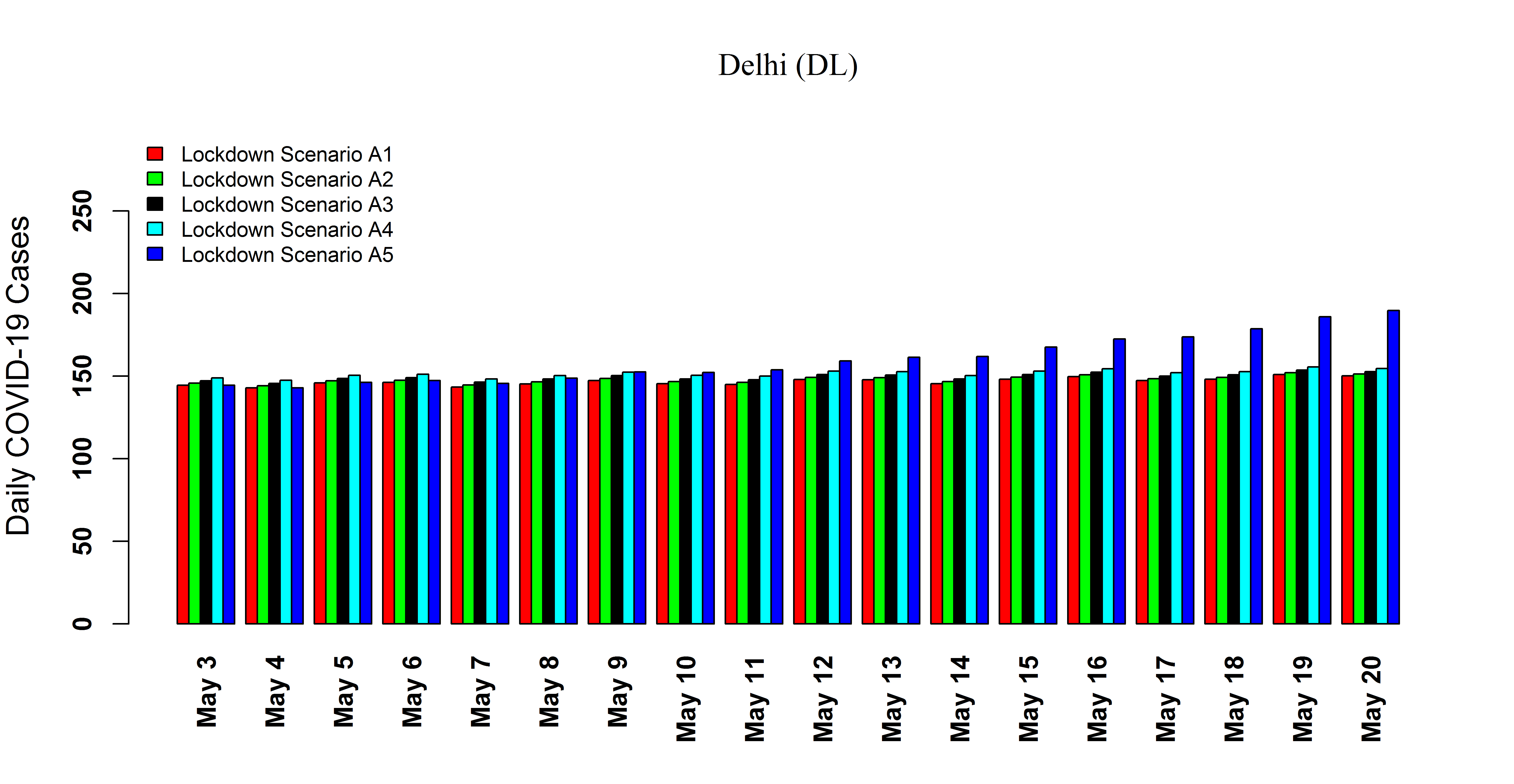
Figure S2: Ensemble model (see main text) forecast for the daily notified COVID-19 cases in Delhi during May 3, 2020 till May 20, 2020 under five different lockdown scenarios. Lockdown Scenarios (A1) to (A5) are same as Figure S1.

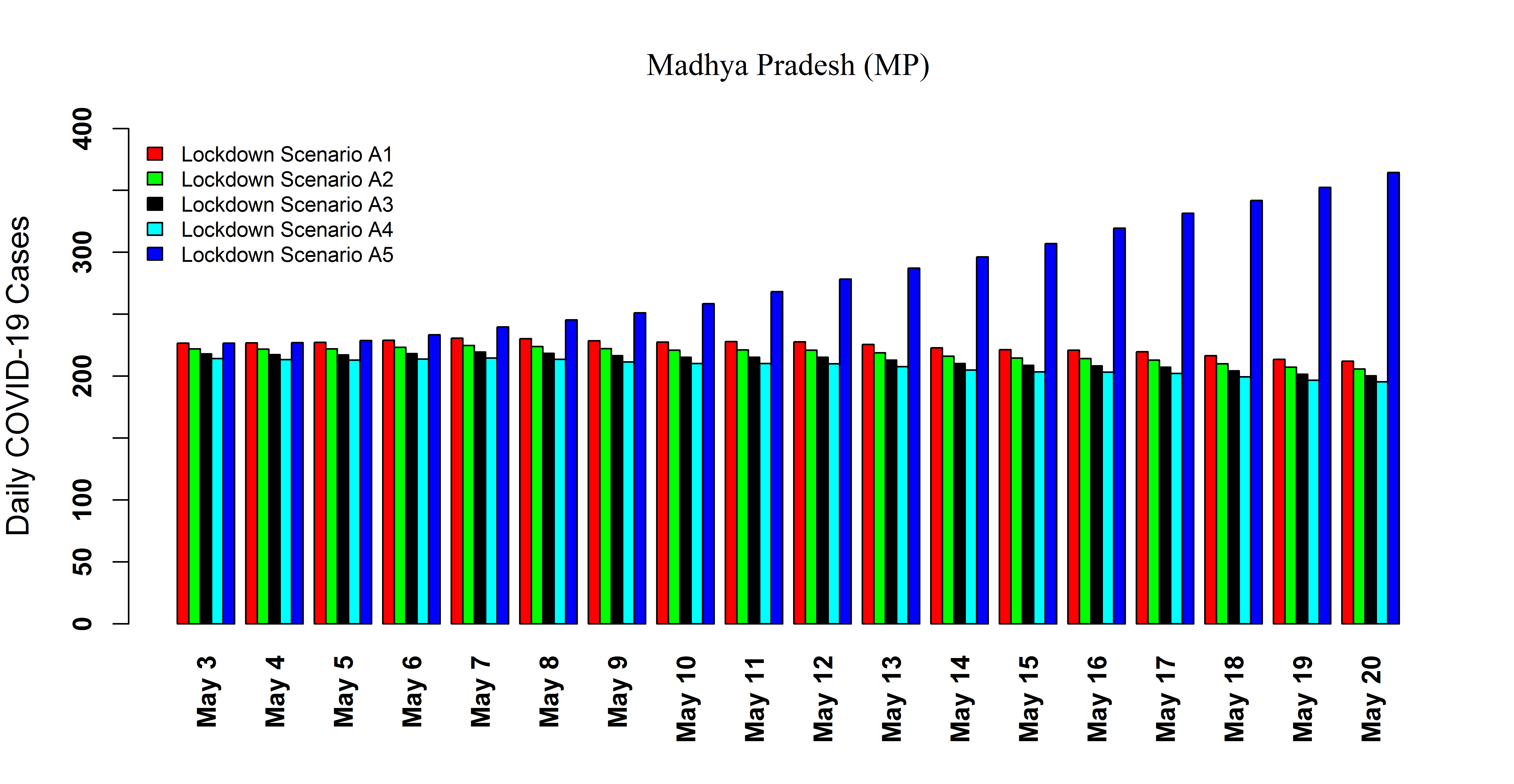
Figure S3: Ensemble model (see main text) forecast for the daily notified COVID-19 cases in Madhya Pradesh during May 3, 2020 till May 20, 2020 under five different lockdown scenarios. Lockdown Scenarios (A1) and (A5) are same as Figure S1. However, under lockdown scenarios (A2) to (A4), projections are made with 10%, 20% and 30% increment in the current estimate of the lockdown rate, respectively (see Table 2 in main text).

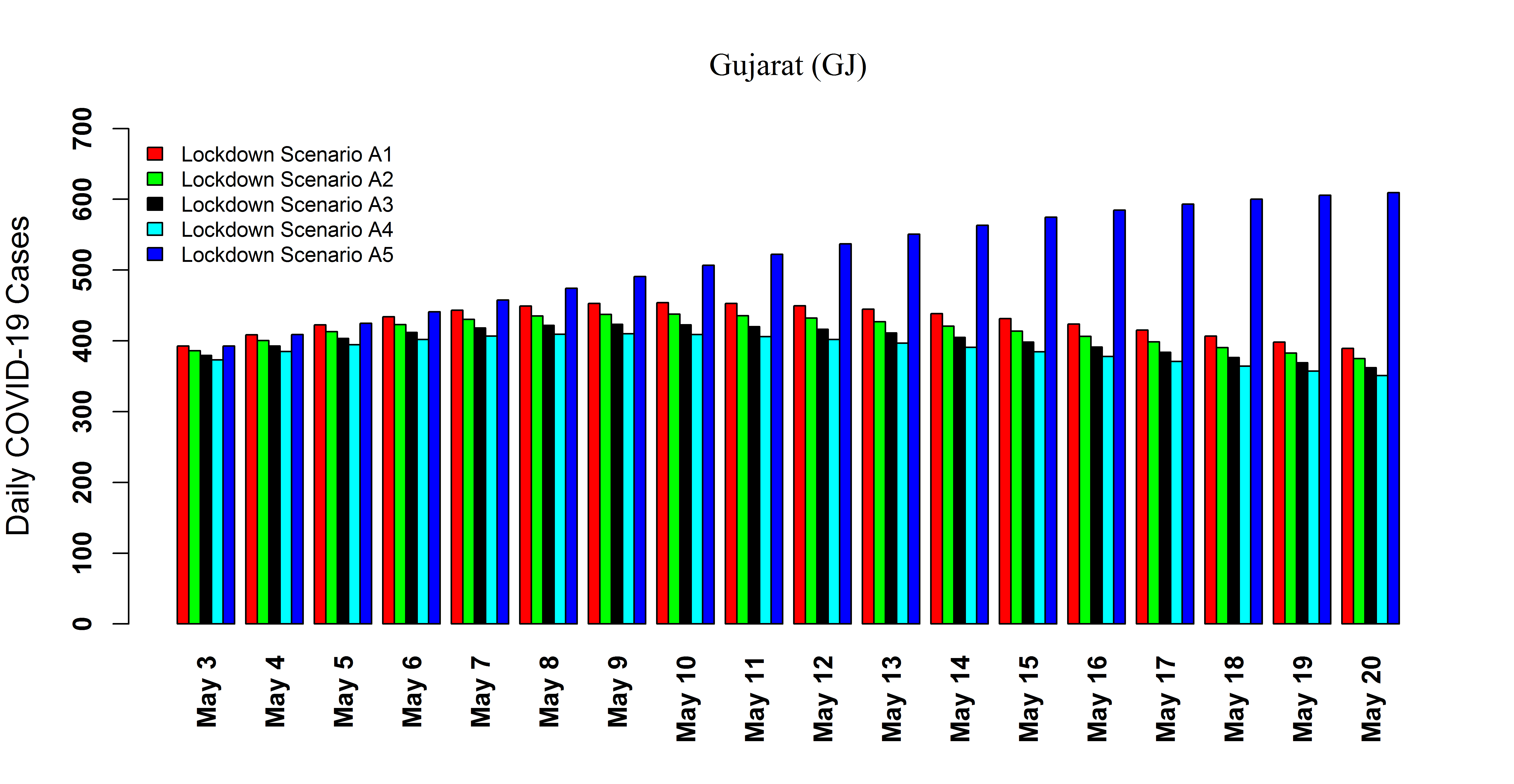
Figure S5: Ensemble model (see main text) forecast for the daily notified COVID-19 cases in Gujarat during May 3, 2020 till May 20, 2020 under five different lockdown scenarios. Lockdown Scenarios (A1) and (A5) are same as Figure S1. However, under lockdown scenarios (A2) to (A4), projections are made with 10%, 20% and 30% increment in the current estimate of the lockdown rate, respectively (see Table 2 in main text).

Figure S11: Effect of uncertainty of four epidemiologically measurable and controllable parameters of the mechanistic ODE model (see Table 1 and Fig 1 in the main text) on the effect of lockdown and the basic reproduction number ($R_{0}$). Lockdown effect is measured in terms of the differences in total number of COVID-19 cases occurred during May 3, 2020 till May 20, 2020 in Gujarat under the lockdown scenarios (A1) and (A5), respectively (see main text). Effect of Uncertainty of these four parameters on the two mentioned responses are measured using Partial Rank Correlation Coefficients (PRCC). $500$ samples for each parameters were drawn using Latin hypercube sampling techniques (LHS) from their respective ranges provided in Table 1 (main text).

Figure S12: Effect of uncertainty of four epidemiologically measurable and controllable parameters of the mechanistic ODE model (see Table 1 and Fig 1 in the main text) on the effect of lockdown and the basic reproduction number ($R_{0}$). Lockdown effect is measured in terms of the differences in total number of COVID-19 cases occurred during May 3, 2020 till May 20, 2020 in Uttar Pradesh under the lockdown scenarios (A1) and (A5), respectively (see main text). Effect of Uncertainty of these four parameters on the two mentioned responses are measured using Partial Rank Correlation Coefficients (PRCC). $500$ samples for each parameters were drawn using Latin hypercube sampling techniques (LHS) from their respective ranges provided in Table 1 (main text).

Figure S13: Posterior distribution of the weights for the mechanistic ODE model combinations (Model without lock-down) & (Model with lock-down) and the Hybrid statistical model (see main text), respectively for Maharashtra.

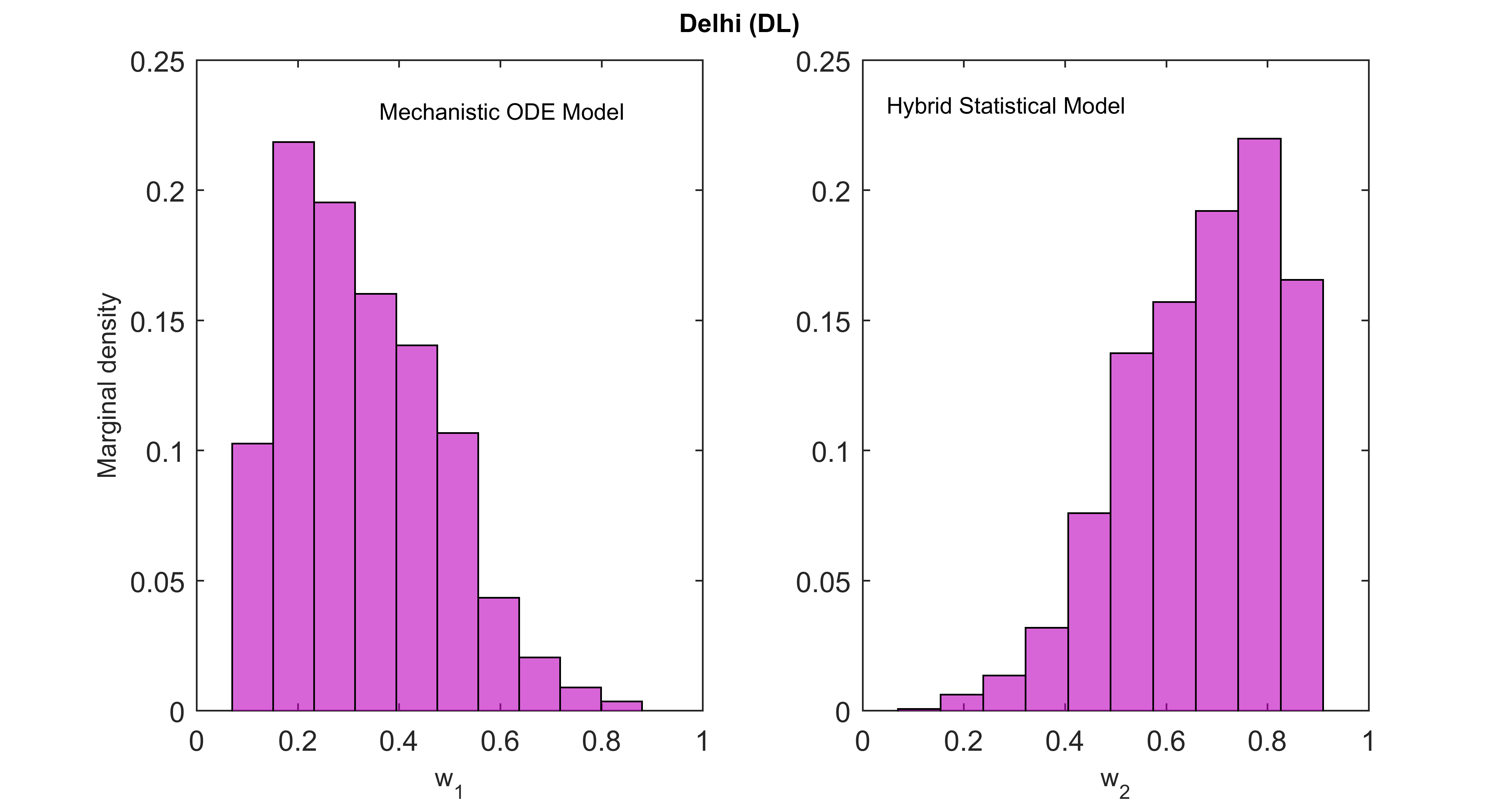
Figure S14: Posterior distribution of the weights for the mechanistic ODE model combinations (Model without lock-down) & (Model with lock-down) and the Hybrid statistical model (see main text), respectively for Delhi.

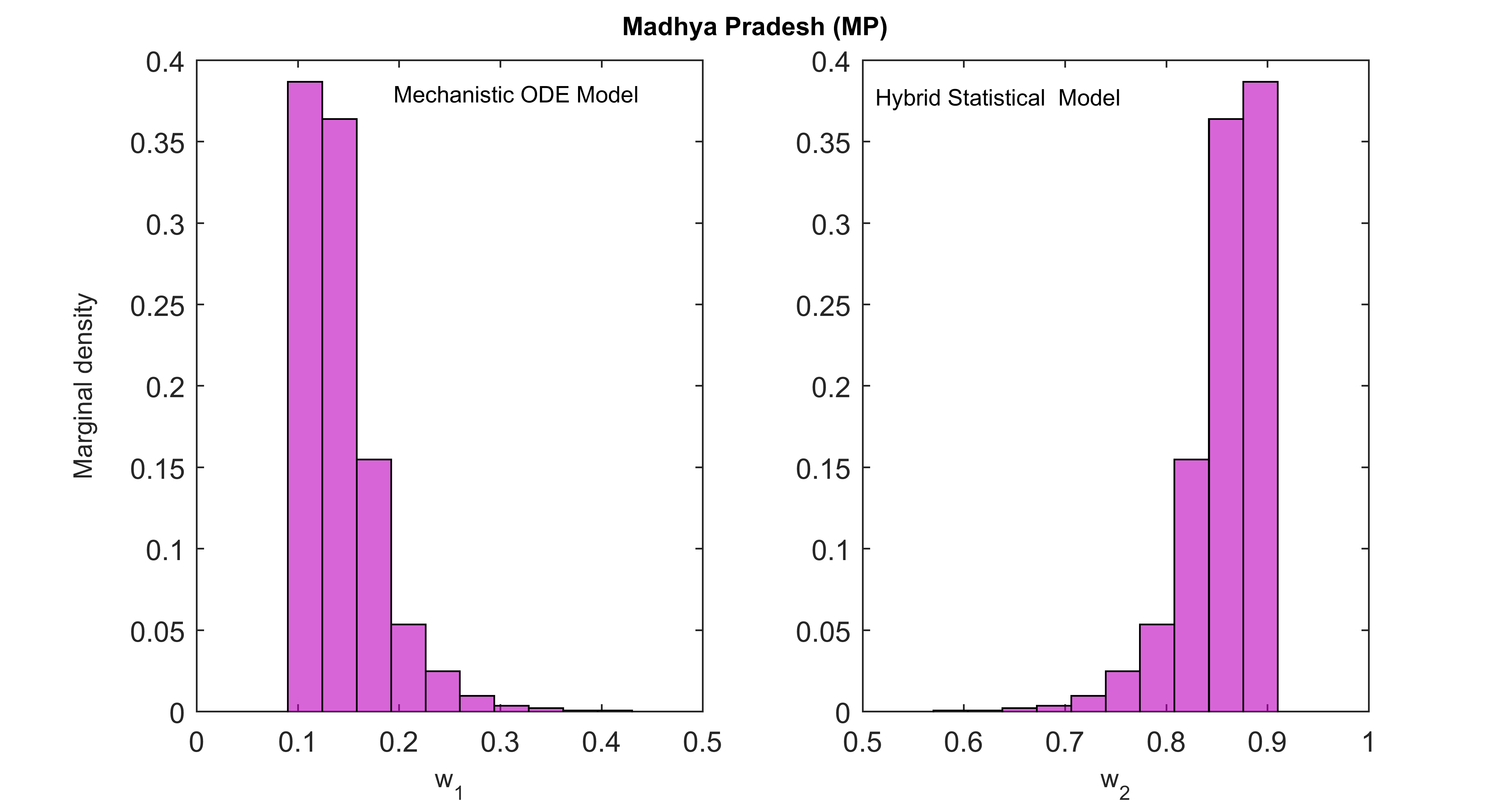
Figure S15: Posterior distribution of the weights for the mechanistic ODE model combinations (Model without lock-down) & (Model with lock-down) and the Hybrid statistical model (see main text), respectively for Madhya Pradesh.

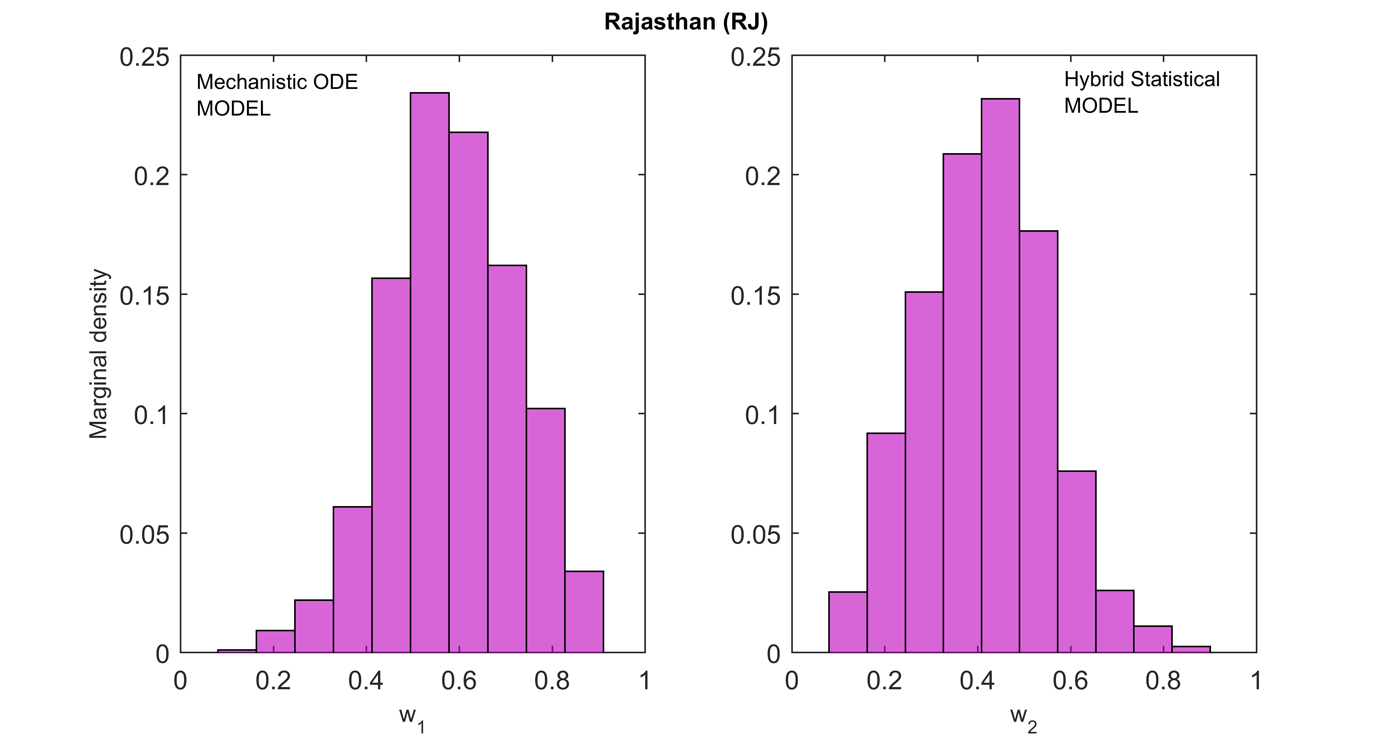
Figure S16: Posterior distribution of the weights for the mechanistic ODE model combinations (Model without lock-down) & (Model with lock-down) and the Hybrid statistical model (see main text), respectively for Rajasthan.

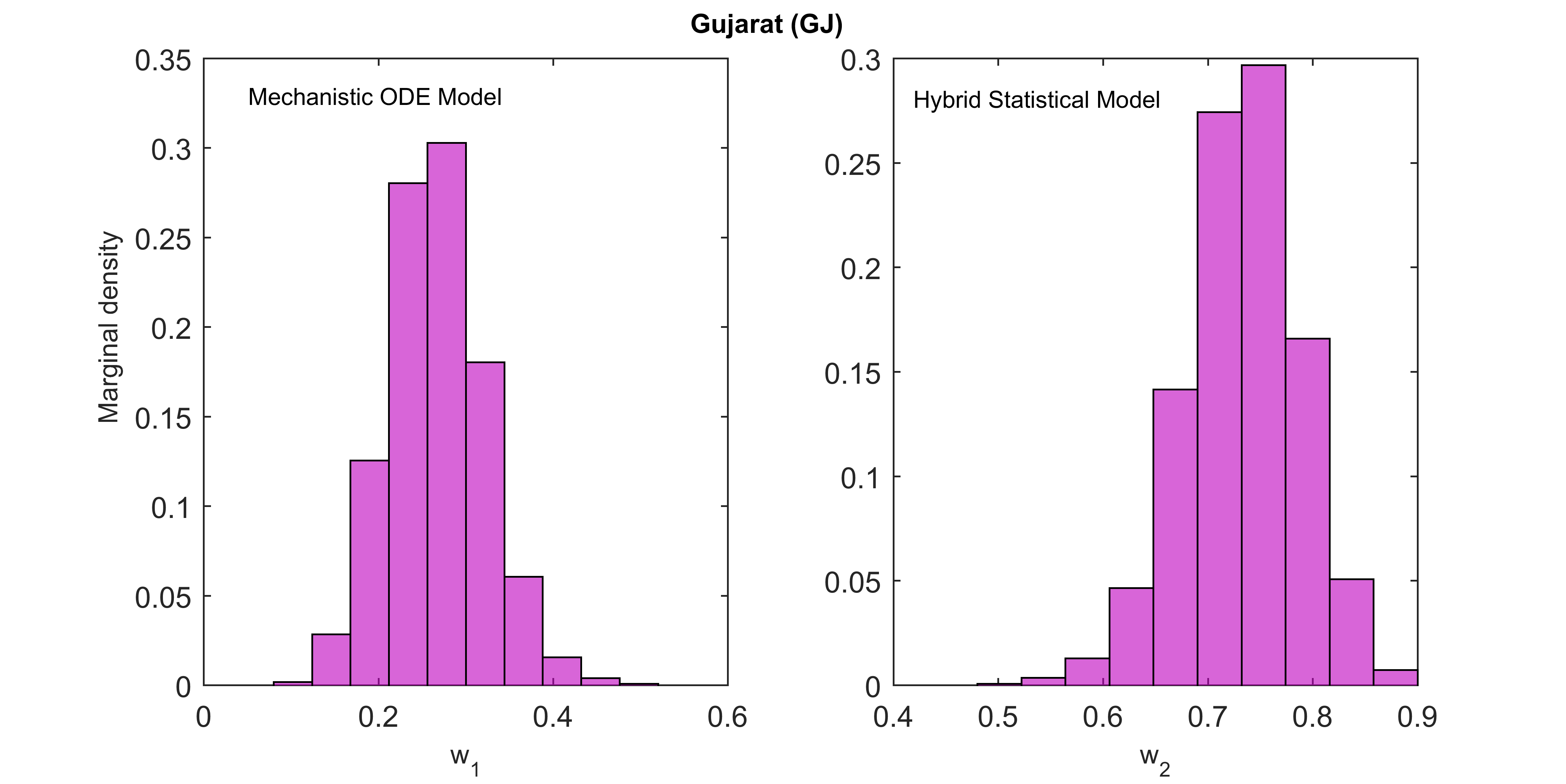
Figure S17: Posterior distribution of the weights for the mechanistic ODE model combinations (Model without lock-down) & (Model with lock-down) and the Hybrid statistical model (see main text), respectively for Gujarat.

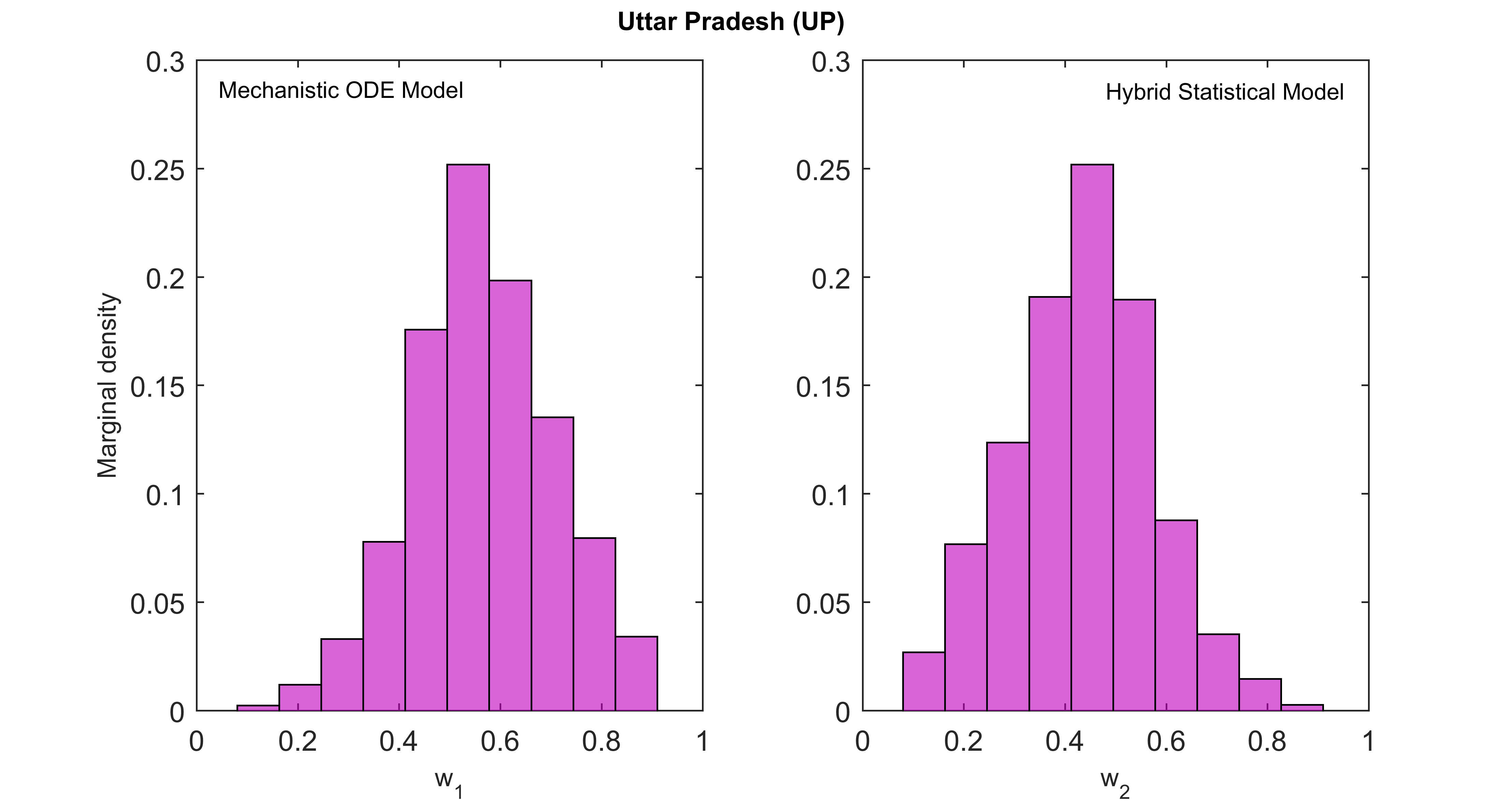
Figure S18: Posterior distribution of the weights for the mechanistic ODE model combinations (Model without lock-down) & (Model with lock-down) and the Hybrid statistical model (see main text), respectively for Uttar Pradesh.

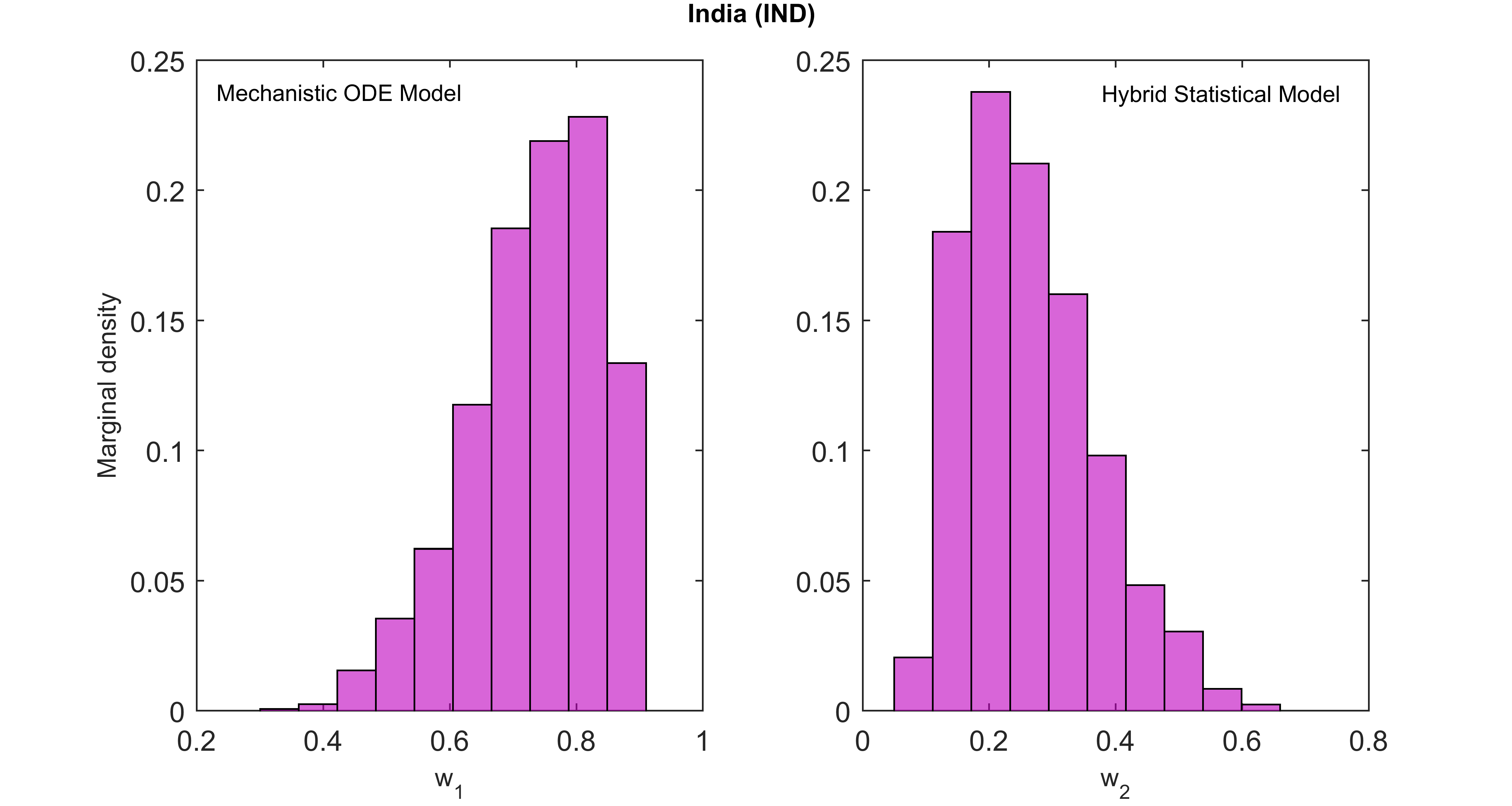
Figure S19: Posterior distribution of the weights for the mechanistic ODE model combinations (Model without lock-down) & (Model with lock-down) and the Hybrid statistical model (see main text), respectively for India.

Tables

Table S1: Estimated uninformative initial conditions for the mechanistic ODE model (Model without lock-down). Respective subscripts are MH: Maharashtra, DL: Delhi, MP: Madhya Pradesh, RJ: Rajasthan, GJ: Gujarat, UP: Uttar Pradesh, and IND: India. All data are provided in the format Estimate (95% CI).

Region	$\boldsymbol{S(0)}$	$\boldsymbol{E(0)}$	$\boldsymbol{I(0)}$	$\boldsymbol{A(0)}$
MH	$\begin{subarray}{c}120428468\\ \\ (101502357-124478508)\end{subarray}$	$\begin{subarray}{c}0.001\\ \\ (0-0.003)\end{subarray}$	$\begin{subarray}{c}332.43\\ \\ (6.14-633.93)\end{subarray}$	$\begin{subarray}{c}2316.93\\ \\ (230.8-7103.05)\end{subarray}$
DL	$\begin{subarray}{c}12173507\\ \\ (10289760-19705021)\end{subarray}$	$\begin{subarray}{c}3743\\ \\ (179-9704)\end{subarray}$	$\begin{subarray}{c}0.14\\ \\ (0-0.29)\end{subarray}$	$\begin{subarray}{c}245\\ \\ (144.5-9409)\end{subarray}$
MP	$\begin{subarray}{c}84632517\\ \\ (70665560-89661041)\end{subarray}$	$\begin{subarray}{c}1541\\ \\ (65.96-4956)\end{subarray}$	$\begin{subarray}{c}0.2914\\ \\ (0.01-1.10)\end{subarray}$	$\begin{subarray}{c}4095\\ \\ (93.46-7852)\end{subarray}$
RJ	$\begin{subarray}{c}74502407\\ \\ (70099616-79723261)\end{subarray}$	$\begin{subarray}{c}195.9\\ \\ (43.74-9770)\end{subarray}$	$\begin{subarray}{c}129\\ \\ (0.7408-132)\end{subarray}$	$\begin{subarray}{c}6209\\ \\ (40.86-9404)\end{subarray}$
GJ	$\begin{subarray}{c}62744520\\ \\ (60628093-69846136)\end{subarray}$	$\begin{subarray}{c}1280\\ \\ (58.78-2238)\end{subarray}$	$\begin{subarray}{c}79.29\\ \\ (3.70-237)\end{subarray}$	$\begin{subarray}{c}1.17\\ \\ (0.39-2.60)\end{subarray}$
UP	$\begin{subarray}{c}224225631\\ \\ (200822802-229090013)\end{subarray}$	$\begin{subarray}{c}0.49\\ \\ (0.01-1.34)\end{subarray}$	$\begin{subarray}{c}3.07\\ \\ (0.17-7.35)\end{subarray}$	$\begin{subarray}{c}4764\\ \\ (379-8031)\end{subarray}$
IND	$\begin{subarray}{c}1219512468\\ \\ (1219512465-1219512469)\end{subarray}$	$\begin{subarray}{c}49998\\ \\ (49995-49999)\end{subarray}$	$\begin{subarray}{c}9997\\ \\ (9994-9999)\end{subarray}$	$\begin{subarray}{c}9995\\ \\ (9991-9999)\end{subarray}$

Table S2: Weight estimates for the mechanistic ODE model combinations (Model without lock-down) & (Model with lock-down) and the Hybrid statistical model (see main text), respectively. Respective subscripts MH, DL, MP, RJ, GJ, UP, and IND are same as Table S1. All data are provided in the format Estimate (95% CI).

Weights	MH	DL	MP	RJ	GJ	UP	IND
$\boldsymbol{w_{1}}$	$\begin{subarray}{c}0.3019\\ \\ (0.2160-0.5284)\end{subarray}$	$\begin{subarray}{c}0.3226\\ \\ (0.1149-0.6594)\end{subarray}$	$\begin{subarray}{c}0.1599\\ \\ (0.0966-0.2384)\end{subarray}$	$\begin{subarray}{c}0.5490\\ \\ (0.3091-0.8384)\end{subarray}$	$\begin{subarray}{c}0.1672\\ \\ (0.1665-0.38)\end{subarray}$	$\begin{subarray}{c}0.6612\\ \\ (0.2807-0.8333)\end{subarray}$	$\begin{subarray}{c}0.8176\\ \\ (0.5017-0.8874)\end{subarray}$
$\boldsymbol{w_{2}}$	$\begin{subarray}{c}0.6981\\ \\ (0.4716-0.7840)\end{subarray}$	$\begin{subarray}{c}0.6774\\ \\ (0.3405-0.8851)\end{subarray}$	$\begin{subarray}{c}0.8401\\ \\ (0.7616-0.9034)\end{subarray}$	$\begin{subarray}{c}0.4510\\ \\ (0.1616-0.6909)\end{subarray}$	$\begin{subarray}{c}0.8328\\ \\ (0.62-0.8335)\end{subarray}$	$\begin{subarray}{c}0.3388\\ \\ (0.1667-0.7193)\end{subarray}$	$\begin{subarray}{c}0.1824\\ \\ (0.1126-0.4983)\end{subarray}$

Table S3: Goodness of fit (RMSE and MAE) of the Hybrid statistical model (see main text) for the test data from MH, DL, MP, RJ, GJ, UP, and IND, respectively. Respective subscripts MH, DL, MP, RJ, GJ, UP, and IND are same as Table S1.

Goodness of fit	MH	DL	MP	RJ	GJ	UP	IND
$\boldsymbol{RMSE}$	$\begin{subarray}{c}35.15368\end{subarray}$	$\begin{subarray}{c}57.855\end{subarray}$	$\begin{subarray}{c}28.59711\end{subarray}$	$\begin{subarray}{c}18.4018\end{subarray}$	$\begin{subarray}{c}21.77785\end{subarray}$	$\begin{subarray}{c}17.60281\end{subarray}$	$\begin{subarray}{c}114.3764\end{subarray}$
$\boldsymbol{MAE}$	$\begin{subarray}{c}22.2375\end{subarray}$	$\begin{subarray}{c}34.4592\end{subarray}$	$\begin{subarray}{c}20.01179\end{subarray}$	$\begin{subarray}{c}13.22069\end{subarray}$	$\begin{subarray}{c}12.91013\end{subarray}$	$\begin{subarray}{c}10.16784\end{subarray}$	$\begin{subarray}{c}65.61564\end{subarray}$

References

- [1] C. Wang, P. W. Horby, F. G. Hayden, and G. F. Gao, “A novel coronavirus outbreak of global health concern,” The Lancet, vol. 395(10223), pp. 470–473, 2020.
- [2] “WHO Director-General’s opening remarks at the media briefing on COVID-19 - 11 March 2020.” https://www.who.int/dg/speeches/detail/who-director-general-s-opening-remarks-at-the-media-briefing-on-covid-19---11-march-2020, 2020. Published on: 2020-03-11.
- [3] “India COVID-19 Tracker.” https://www.covid19world.org/, 2020. Accessed on: 2020-04-28.
- [4] WHO, “Coronavirus disease 2019 (COVID-19), situation report -10.” https://www.who.int/emergencies/diseases/novel-coronavirus-2019/situation-reports/, 2020. Accessed on: 2020-03-25.
- [5] “Coronavirus in India: Tracking country’s first 50 COVID-19 cases; what numbers tell.” https://www.indiatoday.in/india/story/coronavirus-in-india-tracking-country-s-first-50-covid-19-cases-what-numbers-tell-1654468-2020-03-12, 2020. Published on: 2020-03-12.
- [6] “India COVID-19 Tracker.” https://www.covid19india.org/, 2020. Accessed on: 2020-04-10.
- [7] “WHO says over 22,000 healthcare workers across 52 countries infected by COVID-19.” https://health.economictimes.indiatimes.com/news/industry/who-says-over-22000-healthcare-workers-across-52-countries-infected-by-covid-19/75107238, 2020. Published on: 2020-04-12.
- [8] “Why are hospitals hotbeds of COVID-19 transmission?.” https://www.thehindu.com/sci-tech/why-are-hospitals-hotbeds-of-covid-19-transmission/article31386208.ece, 2020. Published on: 2020-04-20.
- [9] “Over 50 doctors, medical staff test positive for COVID-19; govt probing if they got infected from patients.” https://www.indiatoday.in/india/story/over-50-doctors-medical-staff-test-positive-for-covid-19-govt-probing-if-they-got-infected-from-patients-1662917-2020-04-03, 2020. Published on: 2020-04-03.
- [10] “COVID-19 impact: Over 40 nurses test positive in mumbai hospital.” https://economictimes.indiatimes.com/news/politics-and-nation/two-private-hospitals-in-mumbai-sealed-after-staff-test-positive/articleshow/75009359.cms, 2020. Published on: 2020-04-08.
- [11] “89 health dept members, including doctors & IAS officers, test positive for COVID-19 in MP.” https://theprint.in/health/89-health-dept-members-including-doctors-ias-officers-test-positive-for-covid-19-in-mp/403102/, 2020. Published on: 2020-04-16.
- [12] “20 doctors, medics isolated after surgeon tests COVID-19 positive at Aligarh Muslim University.” https://www.ndtv.com/cities/20-doctors-medics-isolated-after-surgeon-tests-covid-19-positive-at-aligarh-muslim-university-2217170, 2020. Published on: 2020-04-23.
- [13] “90 health workers infected with COVID-19, total cases over 8,000 in India.” https://www.ndtv.com/india-news/coronavirus-india-coronavirus-cases-in-india-cross-8-000-mark-34-dead-in-24-hours-2210282, 2020. Published on: 2020-04-12.
- [14] “3 Delhi journalists test COVID-19 positive, says Arvind Kejriwal.” https://www.indiatvnews.com/news/india/coronavirus-delhi-journalist-coronavirus-positive-covid-19-turn-arvind-kejriwal-612422, 2020. Published on: 2020-04-29.
- [15] “COVID-19: Over 50 journalists in Mumbai test positive, says municipal corporation.” https://scroll.in/latest/959732/covid-19-over-50-journalists-in-mumbai-test-positive-says-municipal-corporation, 2020. Published on: 2020-04-11.
- [16] “World’s biggest lockdown may have cost rs 7-8 lakh crore to indian economy.” https://economictimes.indiatimes.com/news/economy/finance/worlds-biggest-lockdown-may-have-cost-rs-7-8-lakh-crore-to-indian-economy/articleshow/75123004.cms?from=mdr, 2020. Published on: 2020-04-13.
- [17] “Coronavirus: 5 indian sectors that need urgent help as virus ravages economy.” https://www.indiatoday.in/business/story/coronavirus-5-indian-sectors-that-need-urgent-help-as-virus-ravages-economy-1670099-2020-04-23, 2020. Published on: 2020-04-24.
- [18] “Red, orange, green zones may come up during extended lockdown.” https://economictimes.indiatimes.com/news/politics-and-nation/red-orange-green-zones-may-come-up-during-extended-lockdown/articleshow/75101054.cms?from=mdr, 2020. Published on: 2020-04-14.
- [19] “Covid-19 lockdown relaxation: Full list of activities allowed from april 20; details.” https://www.financialexpress.com/lifestyle/covid-19-lockdown-relaxation-full-list-of-activities-allowed-from-april-20-details/1933136/, 2020. Published on: 2020-04-19.
- [20] “Coronavirus lockdown India: Does your district fall in ‘red zone’ hotspots? check out full list here.” https://www.businesstoday.in/latest/trends/coronavirus-lockdown-20-does-your-district-fall-in-red-zone-check-out-full-list-here/story/401188.html, 2020. Published on: 2020-04-22.
- [21] S. M. Moghadas, A. Shoukat, M. C. Fitzpatrick, et al., “Projecting hospital utilization during the COVID-19 outbreaks in the united states,” Proceedings of the National Academy of Sciences, vol. 117, no. 16, pp. 9122–9126, 2020.
- [22] B. Tang, X. Wang, Q. Li, N. L. Bragazzi, S. Tang, Y. Xiao, and J. Wu, “Estimation of the transmission risk of the 2019-nCov and its implication for public health interventions,” J. Clin. Med., vol. 9, no. 2, p. 462, 2020.
- [23] T. Sardar, S. S. Nadim, and J. Chattopadhyay, “Assessment of 21 days lockdown effect in some states and overall India: A predictive mathematical study on COVID-19 outbreak,” arXiv preprint arXiv:2004.03487, 2020.
- [24] T. Chakraborty and I. Ghosh, “Real-time forecasts and risk assessment of novel coronavirus (COVID-19) cases: A data-driven analysis,” arXiv preprint arXiv:2004.09996, 2020.
- [25] H. Tandon, P. Ranjan, T. Chakraborty, and V. Suhag, “Coronavirus (COVID-19): ARIMA based time-series analysis to forecast near future,” arXiv preprint arXiv:2004.07859, 2020.
- [26] Z. Hu, Q. Ge, S. Li, L. Jin, and M. Xiong, “Artificial intelligence forecasting of covid-19 in china,” arXiv preprint arXiv:2002.07112, 2020.
- [27] “State/UT wise aadhaar saturation.” https://uidai.gov.in/images/state-wise-aadhaar-saturation.pdf, 2020. Accessed on: 2020-04-10.
- [28] “India will be under complete lockdown for 21 days: Narendra Modi.” https://economictimes.indiatimes.com/news/politics-and-nation/india-will-be-under-complete-lockdown-starting-midnight-narendra-modi/articleshow/74796908.cms?from=mdr, 2020. Published on: 2020-03-25.
- [29] “Lockdown goes from 21 to 40 days, curbs may be conditionally eased in some non-hotspot areas from april 20.” https://timesofindia.indiatimes.com/india/lockdown-goes-from-21-to-40-days-curbs-may-be-conditionally-eased-in-some-non-hotspot-areas-from-april-20/articleshow/75149611.cms, 2020. Published on: 2020-04-15.
- [30] “Coronavirus lockdown 2.0: Till may 3 now, taking total to 40 days.” https://www.financialexpress.com/india-news/coronavirus-lockdown-2-0-till-may-3-now-taking-total-to-40-days/1928585/, 2020. Published on: 2020-04-15.
- [31] H. Haario, M. Laine, A. Mira, and E. Saksman, “Dram: efficient adaptive mcmc,” Statistics and computing, vol. 16, no. 4, pp. 339–354, 2006.
- [32] T. Sardar and B. Saha, “Mathematical analysis of a power-law form time dependent vector-borne disease transmission model,” Mathematical biosciences, vol. 288, pp. 109–123, 2017.
- [33] C. Lemke and B. Gabrys, “Meta-learning for time series forecasting and forecast combination,” Neurocomputing, vol. 73, no. 10-12, pp. 2006–2016, 2010.
- [34] P. Van den Driessche and J. Watmough, “Reproduction numbers and sub-threshold endemic equilibria for compartmental models of disease transmission,” Mathematical biosciences, vol. 180, no. 1-2, pp. 29–48, 2002.
- [35] S. Marino, I. B. Hogue, C. J. Ray, and D. E. Kirschner, “A methodology for performing global uncertainty and sensitivity analysis in systems biology,” Journal of theoretical biology, vol. 254, no. 1, pp. 178–196, 2008.
- [36] “Coronavirus: 80% cases asymptomatic, but no need to revise testing criteria, says ICMR.” https://www.indiatoday.in/india/story/80-of-coronavirus-cases-in-india-are-asymptomatic-icmr-1669073-2020-04-20, 2020. Published on: 2020-04-20.
- [37] “Health systems respond to COVID-19.” http://www.euro.who.int/__data/assets/pdf_file/0006/437469/TG2-CreatingSurgeAcuteICUcapacity-eng.pdf, 2020. Accessed on: 2020-04-30.
- [38] “Life expectancy.” https://niti.gov.in/content/life-expectancy, 2020. Accessed on: 2020-04-10.
- [39] X. Yang, L. Chen, and J. Chen, “Permanence and positive periodic solution for the single-species nonautonomous delay diffusive models,” Computers & Mathematics with Applications, vol. 32, no. 4, pp. 109–116, 1996.
- [40] H. W. Hethcote, “The mathematics of infectious diseases,” SIAM review, vol. 42, no. 4, pp. 599–653, 2000.
- [41] C. Castillo-Chavez, Z. Feng, and W. Huang, “On the computation of R0 and its role on,” Mathematical approaches for emerging and reemerging infectious diseases: an introduction, vol. 1, p. 229, 2002.