A thick-disk galaxy model and simulations of equal-mass galaxy pair collisions

Abstract

We implement a numerical model reported in the literature to simulate the evolution of a galaxy composed of four matter components, such as: a dark-matter halo; a rotating disk of stars; a spherical bulge of stars and a ring of molecular gas. We show that the evolution of this galaxy model is stable at least for 10 Gyr (Gyr=$10^{9}$ years). We characterize the resulting configuration of this galaxy model by figures of the circular velocity and angular momentum distribution; the tangential and radial components of the velocity; the peak density evolution and the radial density profile. Additionally, we calculate several models of equal-mass galaxy binary collisions, such as: (i) frontal and (ii) oblique (with an impact parameter), (iii) two models with initial conditions taken from a 2-body orbits and (iv) a very close passage. To allow comparison with the galaxy model, we characterize the dynamics of the collision models in an analogous way. Finally, we determine the de Vaucouleurs fitting curves of the radial density profile, on a radial scale of 0-100 kpc, for all the collision models irrespective of the pre-collision trajectory. To study the radial mass density and radial surface density profiles at a smaller radial scale, 0-20 kpc, we use a four-parameters fitting curve.

keywords–galaxies: kinematics and dynamics–galaxies: interaction–methods: numerical

1 Introduction

The pioneering work of Toomre at al. (1972) showed that the gravitational interaction between galaxies results in a profound morphological transformation of the participating galaxies and even leads to the formation of new types of galaxies. In that paper, the authors used a dynamic approach, in which the two colliding galaxies were represented as point masses, while the disk of the galaxies was represented with particles that had no gravitational interaction between them. In their simulations, these authors managed to reproduce systems of galaxies in which long lines or bridges appeared, whose similarity with real systems, such as the Antenna galaxy (NGC 4038-39) or the Mice galaxy (NGC 4676), was very encouraging.

Since the 1970s, the simulation of the formation, evolution and interaction of galaxies has been a huge research area of computational astrophysics and continues to be of interest even today, see Athanassoula and Bosma (2019). Although many simulations of galaxy collisions have been carried out over the last few decades, in the first years only gas-free models were considered. Recently, gas began to be included to study its effects. In particular, numerical simulations aimed to follow the gas dynamics in a collision between a pair of comparable-mass galaxies, have a long history. Pioneering works were done by Negroponte and White (1983), in which the gas was represented by spherical particles of variable radius; by Noguchi (1988), in which the influence of the tidal force of a perturbing galaxy on the gas dynamics of the companion galaxy was studied. A new generation of papers, in which the SPH technique was already used, were done by Barnes and Hernquist (1991), Barnes and Hernquist (1996) and Mihos and Hernquist (1996), among others.

The papers Barnes and Hernquist (1991) and Barnes and Hernquist (1996) showed that a strong concentration of gas takes place in the central region of the remnants and for this reason, they argued about the possible occurrence of a starburst in the central region. Noteworthy, Barnes and Hernquist (1996) demonstrated that the gas and the stars showed a different behavior whether the galaxy model evolved as an isolated system or during a galactic collision. Barnes and Hernquist (1996) also noted that the morphology of a merger remnant can be strongly affected by the dynamics of the gas.

Even more recently,  Naab at al. (2006) presented a large set of simulations of uneven-mass galaxy collision models to understand the influence of a gas component on the global structure of mergers remnants. These authors found that the presence of a gas component changes the shape of the merger remnants.  Burkert et al. (2008) also found that some physical properties of the merger remnants depends both on the initial mass ratio of the colliding galaxies and on the gas fraction that they contain.

Numerical simulations of the interaction between a pair of galaxies have been considered in statistical terms by Mateo at al. (2007), who studied a total sample of 240 interactions. They first determined the star formation rate in their galaxy model to then compare these results with those obtained in their models of galaxy interaction. The images they show in their section ”A gallery of galaxy interactions” are impressive, as they were able to compare the time evolution of several matter components of their models, see for instance their Figs. 3,4 and 5.

Gabbasov at al. (2006) presented a rotating galaxy model in which three matter components were included, namely: a dark-matter halo, a spherical star-bulge, and a rotating star-disk. However, they did not include gas in their model. After six times of the rotation period of their galaxy model, the galactic evolution generates a bar, so that their model successfully reproduces the dynamics of a barred spiral galaxy. Subsequently, Luna at al. (2015) (following the work of Gabbasov at al. (2006) presented several collision models in which the spiral bar galaxy introduced by Gabbasov at al. (2006), was the only element of collision. Luna at al. (2015) also did not include gas in their models.

In the present paper, we also follow the galaxy model of Gabbasov at al. (2006) and Luna at al. (2015) regarding the initial dynamics of the three matter components mentioned earlier, but here we also include gas, which is initially distributed as the disk.  Moster at al. (2011) considered a five components galaxy model: dark-matter halo, stellar disk, stellar bulge, gaseous disk and gaseous halo. Consequently, our galaxy model includes a gaseous disk component. It is also important to emphasize that all four matter components considered in this work interact gravitationally and, as expected, the computational cost increases significantly with respect to papers in which the gravitational interaction is modeled or suppressed entirely.

This galaxy model proves to be stable. Therefore, it can be useful to represent the M82 Galaxy, that was originally cataloged as an irregular amorphous galaxy, as reported by Mayya at al. (2009), whose galaxy model showed the formation of an elongated disk-shaped structure in the central region. We characterize the dynamic of this galaxy model by calculating the time evolution of the density peak and the radial density profile of all the matter components at an advanced evolution stage.

It must be noted that the parameter space of hydrodynamical simulations is enormous, even in their most basic implementation, so a new paper can almost always find a new possible variation of these parameters. In the case of this paper, the width of the disk is greater than what is commonly used in many papers.

It should be emphasized that a galaxy model like this is physically possible and interesting, because collisions between galaxies of very different masses can thicken the disk of the most massive galaxy, see Quinn et al. (1993). Villalobos and Helmi (2008) presented SPH simulations to explore the problem of thick disc formation by means of minor collisions between a satellite galaxy hitting on a host galaxy with a pre-existing thin disc. The scaleheight of the initial thin disk is 0.35 kpc while the resulting vertical structure of the thick disk indicates a scaleheight within 1-2 kpc, see their Fig.10.

In this paper we also consider a small sample of equal-mass thick-disk galaxy collision models, like the ones obtained by Villalobos and Helmi (2008), so that we repeat the characterization analysis on the merger remnants, to assess the effects of the collision process on the dynamics of the matter components, particularly on the gas component. We find that the gas forms rapidly rotating structures with a peak density in the central region.

We then calculate the radial density profile of the merger remnants and report the values of the parameters $b_{e}$, $\log(\rho_{e})$ and $R_{e}$ that best fit it by using a de Vaucouleurs function, so that this fitting curve apparently does not depend on the particular geometry of the collision process on a radial scale of 0-100 kpc. It should be noted that  Aguilar and White (1986) found that the de Vaucouleurs surface brightness profile does not change significantly after a couple of galaxies have undergone a tidal encounter, both of which started their evolution with the de Vaucouleurs density profile with other parameters.

There are many empirical formula available in the literature to obtain fitting curves in addition to the de Vaucouleurs, such as the Sérsic function, core-Sérsic, Sérsic-type transition model, Nuker model, for a review see Ferrarese (2006). In addition,  Kormendy at al. (2009) found that the Sérsic functions fit very well the surface brightness profiles of elliptical and spheroidal galaxies in the Virgo cluster. They then tried to distinguish between elliptical and spheroidal galaxies by noting the differences in these fits for small radii, so that these differences can be interpreted as signatures of the galaxy formation mechanism.

These formula are improvements to the de Vaucouleurs function. In spite of this and in addition to the fact that there is no astrophysical reason known to highlight the de Vaucouleurs function over the other formula, we will show in this paper a similar result to that found by  Aguilar and White (1986) that is, the merger remnants manage to take a radial density profile with form of the de Vaucouleurs function, irrespective of the collision model. It must be emphasized that the reconfirmation of this result is now obtained by using a more complete galaxy model, because  Aguilar and White (1986) used 3000 particles per galaxy model. We complement these results with the de Vaucouleurs function, whose details are shown in Appendix A, by testing with another formula in the radial scale of 0-20 kpc, which has given good results as a fitting model for the radial profiles of the HI surface density for 42 galaxies, as Wang et al. (2014) demonstrated recently. These four-parameters fitting function is described in Appendix B.

The rest of this paper is structured as follows. In Sections 2.1 to 2.3, we explain the generation of the initial conditions of the galaxy model. In Section 2.4, we present the evolution code. In Section 3 we show the results obtained: first, for the evolution of the galaxy model in Section 3.1 and second, for the collision models in Section 3.2. A dynamic characterization of the matter components between different collision models is presented in Section 3.3. Some results of this paper are discussed in Section 4. In Section 5 we will try to establish the consistency of the simulations presented in this paper by comparing our main results with other simulations, with observations and with virtual observations as well. Finally, the main conclusions of this paper are summarized in Section 6.

2 The galaxy model

In this paper, we use the SPH (smooth particle hydrodynamics) technique, in which a fluid is represented by a finite set of particles (see Liu (2003) and references there in), so that the galaxy model has four types of particles, one for each type of matter component: halo, bulge, disk and gas. It is important to note that there is a difference between these particle types from the computational point of view, as will be mentioned in Section 2.4.

As usual, each particle must have a mass, a position and a velocity at time $t=0$. We show in Sections 2.1,2.2 and 2.3, how the mass, the positions and finally, the velocities are assigned, respectively.

2.1 Initial mass of particles

Because the total mass of each component of the galaxy model is very different, the number of particles will also be very different. This is mainly because we want to use only a single magnitude of elementary mass for all the matter components. It is shown elsewhere that the simulations of this kind produce better computational results than those with particles having very different elementary masses.

In Table 1, we list the matter component and its properties, as follows. To achieve the total mass per matter component given in column 3, the mass of the elementary particle, which is of 412,500 $M_{\odot}$, must be multiplied by the number of particles given in column 2. The fractions that this matter component represent in the entire galaxy model are shown in column 4.

The total number of particles in the galaxy model is 676237, such that the total mass is 2.79 $\times 10^{11}\,M_{\odot}$ that extends over a sphere of radius of 240 kpc. The average density of the system is $3.02\times 10^{-28}$ g/cm³.

The masses reported in Table 1 were suggested in the papers by Gabbasov at al. (2006) and Luna at al. (2015). The meaning of the other columns of Table 1 are explained below.

Table 1: Parameters of the galaxy model.

matter	number of	total mass	mass fraction	initial radial	final radial	a [kpc]
component	particles	[$M_{\odot}$]		extension [kpc]	extension [kpc]
gas	10000	4.12$\times 10^{9}$	0.0147	16-20	180	–
disk	99950	4.12$\times 10^{10}$	0.147	0-16	60	3.3
bulge	33205	1.4$\times 10^{10}$	0.049	0-60	160	1.66
halo	533082	2.2$\times 10^{11}$	0.788	0-240	$\geq$ 200	4

2.2 Initial position of particles

The Monte Carlo method is used, so that the particles are located randomly in the space available of the galaxy model. In column 5 of Table 1, we show the initial radial extension achieved by the initial distribution of particles. The number of particles in a ring of radial width $R$ and $R+\delta R$ is determined to satisfy the radial density profile that has been reported in the literature. For example, for the dark-matter halo, we use the density profile reported by Dehnen (1993), which includes the length parameter $a_{h}$. For the bulge we use the profile reported by Hernquist (1990), which also includes a parameter of length $a_{b}$; for the disk we use the formula reported by Freeman (1970), with a length parameter $a_{d}$. The length parameter $a$ determines the radius in which the density curve falls with respect to the radius of the galaxy. The values of these parameters are reported in column 7 of Table 1. It should be emphasized again that these formulas have been taken from the papers of Gabbasov at al. (2006) (see equations 1, 2 and 3) and Luna at al. (2015) (see equations 1, 2 and 3) and therefore we do not reproduce them again here.

The gas particles were initially located between an inner and outer radii, so that the gas particle radius is always greater than the initial radial extent of the star disk reported in column 5 of Table 1 and smaller than the radial limit of 20 kpc. In other words, the gas was uniformly distributed in a ring in the range 16–20 kpc. In this case, there is no parameter $a_{g}$, as reported in Table 1. The width of the star disk must also be specified, which was set in this work at the value of $z_{0}$ = 1 kpc.

The gas component can be located initially forming a ring, as is usually observed to be in spiral galaxies, see Schneider (2006). The typical inner and outer radii of this molecular gas ring for spiral galaxies are 3 kpc $<$ R $<$ 8 kpc with an scale-height of 0.09 kpc. Atomic hydrogen gas can be observed up to a radius of $R<25$ kpc with a scale-height of 0.2 kpc. However, as we mentioned in Section 1, in this paper we consider the case of a thick disk of gas, which can be the result of several collisions between a large disk and small companions, as was modeled by Quinn et al. (1993), who demonstrated that the original disk is not destroyed (as usually happens in the case of major mergers) but is slowly disturbed, so that the resulting disk spreads in radius and inflates vertically until it eventually settles into a new equilibrium configuration. For this reason, the ring of gas in this paper has initially been located as explained above.

2.3 Initial velocity of particles

We determine the initial velocities of the particles by means of a distribution function. For example, assuming that the halo and bulge are isotropic, they then follow a Maxwell distribution function, with only a radial velocity dispersion, denoted by $\sigma_{r}$, which determines the opening of the distribution function curve (a Gaussian curve). In general, the radial dispersion of the velocity for the halo and bulge depends on the radial coordinate of the galaxy. For anisotropic cases, velocity dispersions in all coordinate directions must also be included, for example, in spherical coordinates with $\theta$ and $\phi$ the azimuthal and polar angles, then $\sigma_{\theta}$ and $\sigma_{\phi}$ are the velocity dispersions needed. In this work, as a first approximation, we only consider isotropic velocity distributions for the halo and bulge (see equations 4 and 6 of the paper by Luna at al. (2015)).

Likewise, it should be emphasized that we use the escape velocity, defined by $V_{\rm esc}=\sqrt{2\,G\,M(R)/R}$, of each matter component as an upper limit of velocity magnitude in the velocity distribution function. Here, $M(R)$ is the total mass of each matter component contained up to the radius $R$ and $G$ is Newton’s gravitational constant.

This means that all velocities greater than the escape velocity were re-defined with the value of the escape velocity. Consequently, we consider that the resulting velocity distribution may be characterized by comparing the average velocity of each matter component with its corresponding escape velocity, see Table 2.

Table 2: The average velocity of the galaxy model obtained from a distribution function.

matter	escape velocity	average velocity
component	[km/s]	[km/s]
gas	42	13
disk	148	106
bulge	44	30
halo	88	87

The particles of the disk have an assigned angular velocity, the value of which depends on the radial coordinate of the particle and the value of its gravitational potential in that radial coordinate. We emphasize that the average value of the angular velocity of the disk particle distribution is $1.3\times 10^{-16}$ radians per second.

The velocity distribution functions for the disk are characterized by three dispersion functions, in cylindrical coordinates $(r,\theta,z)$ these are $\sigma_{r}$, $\sigma_{\theta}$ and $\sigma_{z}$. The velocity dispersion in the radial coordinate depends on the value obtained from the angular velocity and the radius of the disk, so that the mathematical formula was taken from the article by Hohl (1971) (see his equation 8).

Following the papers of Gabbasov at al. (2006) and Luna at al. (2015), the velocity dispersion in the $z$ coordinate, $\sigma_{z}$, is given in terms of the radial dispersion, as follows $\sigma_{z}=\sigma_{r}/2$. Following the paper by Hohl (1971), the dispersion of the velocity in the tangential direction becomes equal in magnitude to the radial dispersion, thus $\sigma_{\theta}=\sigma_{r}$. These choices are somewhat arbitrary and can be changed according to the galactic dynamics desired. In this case, the galaxy model rotates differentially (not as a rigid body), with the Z-axis as the axis of rotation, so that the rotation period of the galaxy is about 1.5 Gyr.

The gas component described in Section 2.2, was endowed with a radial velocity dispersion similar to the disk, except that we now use the average angular velocity of the disk for all of the gas particles, rather than the angular velocity at each radial position of the particle. With this procedure, we try that the ring of gas rotates as a rigid body with constant angular velocity. The tangential component of the velocity of each particle increases linearly with its radius and is proportional to a constant, which is called the epicyclic frequency of the system, see for example equations 6–63 on page 371 of  Binney and Tremaine (1994).

In Fig. 1 we show the initial configuration of all the particles for three matter components, because the dark-matter halo is not shown. The evolution of these initial conditions is carried out using the public code Gadget2, which is presented in Section 2.4. The initial conditions were evolved up to 10 Gyr or equivalently, for almost 6.6 times the rotation period of the galaxy model. To carry out this evolution, almost 200 hours of computation were necessary running in parallel in 40 processors of the Cuetlaxcoapan Supercomputer of the LNS-BUAP. The results obtained are presented below in Section 3, by means of figures in which the matter components are shown separately by a color set, assigned by the public code see  Paraview (2013).

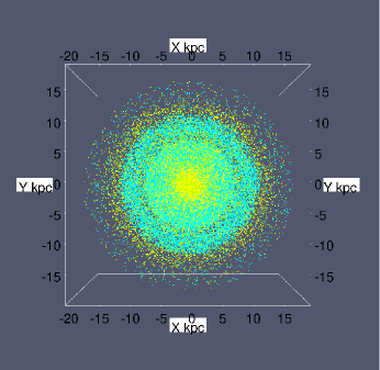
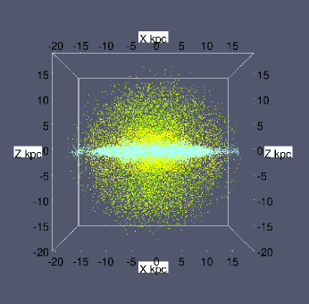
Figure 1: Initial configuration for all the particles at time t = 0 of the three matter components: a view of the XY plane is shown in the left panel, while a view of the ZX plane is shown in the right panel. The region shown is within the interval (-20,20) kpc for the X-axis, the Y-axis and the Z-axis. The colors indicate the matter components according to bulge-yellow, gas-green and disk-blue.

2.4 The evolution code

In this paper, we use the particle-based code Gadget2, which is based on the tree-PM method for computing the gravitational forces and on the standard SPH method for solving the Euler equations of hydrodynamics, see Springel (2005). The Gadget2 program has implemented a Monaghan–Balsara form for the artificial viscosity, see Balsara (1995). The strength of the viscosity is regulated by setting the parameter $\alpha_{\nu}=0.75$ and $\beta_{\nu}=\frac{1}{2}.\times\alpha_{v}$, see equations 11 and 14 in Springel (2005). We have fixed the Courant factor to be $0.1$.

In Gadget2, the SPH sums are evaluated using the spherically symmetric M4 kernel and so gravity is spline-softened with this same kernel. There is a smoothing length, denoted here by $h$, which establishes the compact support, so that only a finite number of neighbors to each particle contribute to the SPH sums. In particular, each particle has its own smoothing length, which evolves with time so that the mass contained in the kernel volume is a constant for the estimated density. Particles are also allowed to have individual gravity softening lengths, denoted by $\epsilon$, which evolve in step with the smoothing length $h$, so that the ratio $\epsilon/h$ is of order unity. The $\epsilon$ determines the smallest possible separation for two individual particles, so that the spatial resolution of a simulation is set by the choice of $\epsilon$. In Gadget2, $\epsilon$ is set equal to the minimum smoothing length $h_{\rm min}$, calculated over all particles at the end of each time step.

As we mentioned at the beginning of Section 2, there are six types of particles defined in the Gadget2, which are labeled from 0 to 5. When the gravitational interaction is computed, all the of particles are treated in the same way by the Gadget2, irrespective of the particle type. However, it is allowed that each particle type can have a different gravitational softening.

In this paper, the gas particles have been assigned the Gadget2’s particle type 0; in this case, there is an hydrodynamical force to be calculated in addition to the gravitational force, so that the former includes a pressure gradient generated by differences in the spatial distribution of the thermal pressure field. Consequently, these particles are considered as collisional particles.

All of the other particle types of the Gadget2 are considered as collision-less particles. Thus, the dark-matter particles have been assigned the Gadget2’s particle type 1, which means that they are treated as collision-less particles of unknown nature. The disk particles have been assigned a Gadget2’s particle type 2. The bulge particles have been assigned the Gadget2’s particle type 3, so that the disk and the bulge are both composed of collision-less stars, but the Gadget2 allows them to have different masses.

However, due to our implementation procedure based on an elementary mass particle, described in Section 2.1, in this paper the only difference between the disk and bulge components is the number of elementary particles that are used to represent their total masses, see Table 1.

Finally, it should be noted that there are no other differences between these particle types in addition to their collision or collision-less nature. Moreover, this paper has not considered the Gadget2’s particle type 4, labeled in the code as ”Stars”, which allows the implementation of a star formation algorithm. Gadget2’s particle types will be very useful in Section 3, where plots will be presented in which the particle types are handled separately, so that we will follow the spatial distribution of each particle type in both the galaxy model and in the collision models.

3 Results

3.1 Evolution of the galaxy model and its dynamic characterization

In Fig. 2, we show the evolution obtained from the galaxy model up to 9.8 Gyr time or equivalently, to 6.5 times the rotation period of the galaxy model. It is seen that the overall system has developed an elongated shape in the central region. The disk has also experienced an expansion in its central region. However, at the ends there is and additional extension in the form of a bow tie, which can be seen in the left-hand bottom panel of Fig. 2. The right-hand bottom panel Fig. 2 indicates that the disk keeps its elongation along XY plane, such that in the ZX view, and it still looks like a thick disk. The bulge keeps wrapping the central part of the disk.

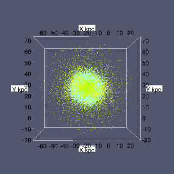
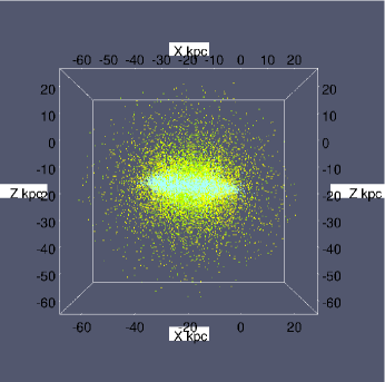
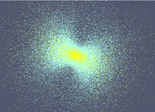
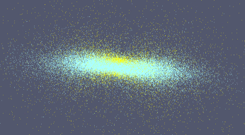
Figure 2: At time t = 9.8 Gyr, equivalent to 6.5 times the rotation period of the galaxy model, we show a XY view at the top left panel and a ZX view at the top right panel. The region shown is within the interval (-60,20) kpc in all the axes. Two amplifications of these panels are shown in the panels on the line below, respectively, so that the region amplified is now within the interval (-40,0) kpc in the X-axis, (0,40) kpc in the Y-axis and (-20,0) kpc in the Z-axis. The colors indicate the matter components according to bulge-yellow, gas-green and disk-blue.

3.1.1 The circular velocity profile and the time evolution of the angular momentum for the galaxy model.

To characterize the mass distribution obtained at the evolution end of the galaxy model, in the left-hand panel of Fig. 3 we show the circular velocity curves of the galaxy model, so that the matter components are considered separately. It must be clarified that to make this plot, we take a radial partition of the galaxy model in $n_{\rm bin}$ bins, starting from the center of mass of each matter component, up to a maximum radius of 100 kpc. Next, we accounted for all the particles contained in each radial bin by taking into account their matter component type, so that the total mass $M(R)$ of each matter component contained up to the radius $R$, is calculated, and we then get the circular velocity, which is defined as $V_{\rm cir}=\sqrt{G\,M(R)/R}$, where $G$ is Newton’s gravitational constant and $R$ is the radius shown on the horizontal axis. The curve labeled ”all” includes all the particles irrespective of their matter component type.

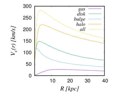
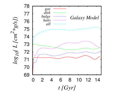
Figure 3: (left) Circular velocity of the galaxy model at time t = 13.7 Gyr. (right) The magnitude of the angular momentum L, in cgs units. On the horizontal axis, the evolution time in Giga-years. Each curve of both panels is generated by taking into account the center of mass of each matter component separately.

The velocity curves reach their maximum velocity at a very small radius; for greater radii, the curves fall very quickly as the distance to the center of the galaxy increases. Gas is an exception because its circular velocity curve remains practically constant for every radius greater than 10 kpc. It is must be emphasized that both the bulge and the gas have been extended spatially to a scale of 160 and 180 kpc, respectively. The disk remains more concentrated in the central region of the galaxy model, but some part of it reaches a length extension of 40 kpc.

These curves can be compared with those calculated by Kuijken at al. (1995) (see his Figure 4) who reports rotation curves with very pronounced drop for the bulge and the disk. It should be emphasized that the observations of the rotation curves of the M82 galaxy, reported by Mayya at al. (2009) also show a very pronounced drop, just as this galaxy model does in this work.The shape of the circular velocity curves obtained in this paper are similar to those obtained by  Meza at al. (2003), in which the formation of an elliptical galaxy in a cosmological simulation is calculated.

In the right-hand panel of Fig. 3 we show the time evolution of the magnitude of the total angular momentum for the galaxy model. We emphasize that the magnitude $L$ was calculated using all the particles in the simulation, and in the case of the curve labeled ”all”, irrespective of the matter component type. To take into account the type of the matter component separately in the calculation of the angular momentum for the galaxy model, so that the other four curves of the right-hand panel of Fig. 3 must be now considered.

For the galaxy model, we observe that all these matter components have zero initial angular momentum (extrapolating the behavior of the curve near the origin of coordinates) except for the disk, whose angular momentum was given initially a non-zero value. However, in less than 2 Gyr of evolution, all these matter components very quickly acquire a significant total angular momentum that is comparable in magnitude to the angular momentum of the disk.

Although the total mass of the gas is considerably smaller than the total mass of the other matter components, the gas follows a circular movement and rapidly gains angular momentum. Its angular momentum is clearly smaller in magnitude than of the rest of the components. Nevertheless, its magnitude is very significant, because it indicates that its angular velocity should be very large.

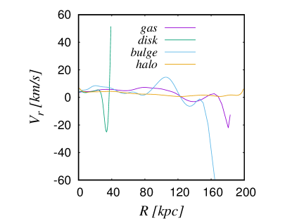
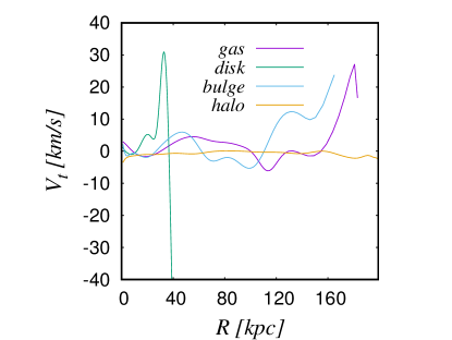
Figure 4: At the same time of Fig. 3, in the left panel we show the radial component of the velocity and in the right panel the corresponding tangential component of the velocity.

In Fig. 4, we show the radial and tangential components of the velocity for each matter component of the galaxy model. It can be seen that the disk maintains its initial nature of a rotating rigid body. Meanwhile, the other components, such as the halo and the bulge, do not show any appreciable circular movement. It should be noted that the radial length extended as much as was necessary, to take into account the radial bins where there were still particles.

3.1.2 Time evolution of the density peak and radial density profile for the galaxy model

In the left-hand panel of Fig. 5, we show the time evolution of the peak density for the gas component up to 4 Gyr of evolution, despite the fact that the final snapshot was taken at a time of 13.7 Gyr. Therefore, this panel will be useful for comparison with the characterization of the collision models to be presented in Section 3.2 and whose results will be discussed in Section 3.3.1.

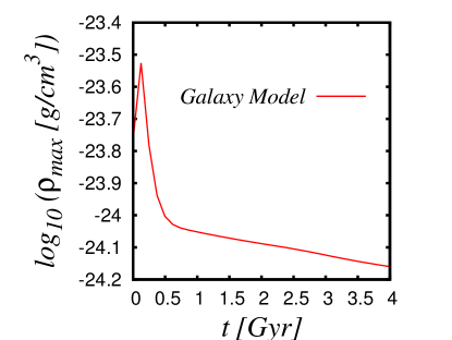
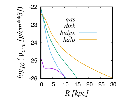
Figure 5: At time t = 13.7 Gyr, we show (left panel) the time evolution of the peak density for the gas component and (right panel) the radial density profile for each matter component of the galaxy model.

Recall that in the galaxy model considered in this paper, the gas component is initially located in a ring with radii in the range within 16 to 20 kpc. The left-hand panel of Fig. 5 indicates that the gas get moved rapidly towards the central region of the galaxy model and then get expanded radially, so that the final radial extension of the model is in the range of 0–180 kpc, see column 6 of Table 1

In the right-hand panel of Fig. 5, we show the radial density profile for each matter component of the galaxy model up to a radius of 100 kpc, despite the fact that in the final snapshot most of the particles are concentrated within a radius of 80 kpc. This is done in this way to allow comparison with the characterization of the collision models to be discussed in Section 3.3.1.

As indicated in the right-hand panel of Fig. 5, there is a strong concentration of all types of matter in the center of the galaxy and to the extent that we move away from the center– say in radii greater than 40 kpc - the density drops up to 7 orders of magnitude. These curves can be compared with those calculated by Kuijken at al. (1995). In addition, it should be remembered that the average density of the system is 3.02 $\times 10^{-28}$ g/cm³, so it should be noted that the increase in density in the central region of the galaxy model is of 5 orders of magnitude; that is, it reaches up to 3.0 $\times 10^{-23}$ g/cm³.

It should be noted that the curves for the gas and bulge are very similar for large radii, except in the central region, so that for a radius smaller than 10 kpc, the curve of the bulge is steeper than the curve of the gas, as can be seen in the right-hand panel of Fig. 5. In addition, the curve for the disk falls very quickly with the radius while the curve for the halo falls softly.

We have determined the extreme spatial extension of each component by the end of the simulation. We found that the gas has reached a huge spatial expansion; on the contrary, the disk component remains more or less bounded to the center. It should be noticed that the bulge component has expanded more than the disk component. Consequently, the gas density is obviously lower than the density of the other mass components, as the gas spreads at large radii from the galaxy center.

Then, based on the results shown both in the left-hand panel of Fig. 3 and in the right-hand panel of Fig. 5, it can be concluded that all of the matter components of the galaxy model are strongly concentrated in the central region, so that the mass contained up to the radius $R$ grows very quickly with the radius. In fact, for radii a little smaller than 10 kpc from the galaxy center, the total mass contained has already reached their asymptotic value, and for this reason, all the curves shown in the left-hand panel of Fig. 3 decrease as $1/\sqrt{R}$ for large $R$.

It has been observed that the galaxy model is stable after almost 10 rotation periods of evolution (equivalent to 14 Gyr of evolution) because it has reached a state of dynamic equilibrium.

3.2 Models of galaxy collision.

The most important application of the basic galaxy model characterized in Section 3.1 is the study of collision models between equal-mass galaxies. In this paper we only consider a few collision models, which are described below and summarized in Table 3. The evolution of each collision model was carried out with the public code Gadget2 described in Section 2.4, during 100 hours of CPU, running in parallel with 20 processors of the Cuetlaxcoapan Supercomputer of the LNS-BUAP.

Table 3: Models of galaxy collisions.

model	impact parameter	initial positions	initial velocities
	[kpc]	$(x,y,z)_{1}$ and $(x,y,z)_{2}$ [kpc]	$(vx,vy,vz)_{1}$ and $(vx,vy,vz)_{2}$ [km/s]
S02	0	(-200,0,0);(200,0,0)	(75,0,0);(-75,0,0)
S02b	100	(-200,0,-50);(200,0,50)	(75,0,0);(-75,0,0)
Orb	0	(-197,0,0);(197,0,0)	(0,-6.19,0);(0,6.19,0)
Tom	20	(20,-20,0);(0,0,0)	(0,136,136);(0,0,0)
Rot	0	(-90,49,0);(90,-49,0)	(31.3,-6.39,0);(-31.3,6.39,0)

In the first two models of Table 3, two equal-mass galaxies are initially separated by almost 400 kpc along the X-axis, so that the galaxies move with respect to each other with an initial translation velocity of 75 km/s, such that the approach velocity before the collision is 150 km/s.

In the case of the model S02, both galaxies collide directly, so that a merging process starts at a time of 1.76 Gyr of evolution, in which the center of mass of each galaxy are very close to each other. The merging process seems to finish at the time of 2.1 Gyr, in which one sees only one center of mass oscillating along the X-axis. Fig. 6 shows a snapshot of the merging process of both galaxies at a time of 1.9 Gyr. It is interesting to note that the gas and bulge expand spatially during both the pre-collision period of translation and the merging process. It is also interesting to mention that the disk remains elongated in the new galactic structure formed after the collision.

In the case of the oblique collision model S02b, both galaxies are additionally displaced a distance of 50 kpc along the Z axis. Consequently, this separation acts as an effective impact parameter of 100 kpc for the collision model (this is the only difference with respect to the frontal collision model S02). The galaxies move along the X-axis, so that the point of maximum pre-collision approach is reached at the time of 2 Gyr of evolution. The galaxies enter in orbit one with respect to the other, as shown in Fig. 7, in which the evolution time increases from the top panel to the bottom panel.

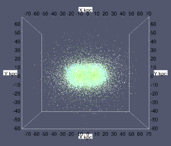
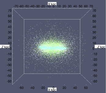
Figure 6: Coalescence of the collision model S02 at the time 1.9 Gyr equivalent to 1.26 times the rotation periods of the galaxy model; the XY view is displayed on the left panel while the ZX view is shown on the right panel. The region shown is within the interval (-70,70) kpc in the X-axis, (-60,60) in the Y-axis and (-70,70) in the Z-axis. The colors indicate the matter components according to bulge-yellow, gas-green and disk-blue.

Around an evolution time of 2.5 Gyr, the binary system has made a complete turn over its orbit. By the time of 2.75 Gyr, the galaxies of the binary system start separating again. We follow the evolution of the model S02b up to a time of 6.54 Gyr, equivalent to 4.3 times the rotation period of the galaxy model. We do not observe a subsequent approach of the galaxies. Therefore, it is very likely that this system is not sufficiently bound to maintain its galaxies in orbit, so that a galaxy will eventually escape from the gravitation field of the other. It is again interesting to mention that the disk remains elongated while the bulge has spread to connect both disks during their orbital motion.

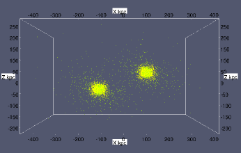
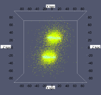
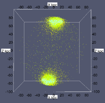
Figure 7: The ZX view of the oblique collision model S02b. In the top panel the 100 kpc length lever arm is seen implemented along the Z-axis; the approach speed is 75 km/s on each side; it corresponds to an evolution time of 0.86 Gyr, which is equivalent to 0.57 times the rotation period of the galaxy model; the region shown is (-400,400) kpc in the X-axis and (-200,200) in the Z-axis. The middle panel corresponds to 2.0 Gyr or equivalent to 1.3 times the rotation period of the galaxy model. The bottom panel corresponds to 3.1 Gyr or 2 times the rotation period of the galaxy model. The region shown in both the middle and bottom panels is (-80,80) kpc both in the X-axis and in the Z-axis. The colors indicate the matter components according to bulge-yellow, gas-green and disk-blue.

The initial conditions of the collision model labeled Orb in Table 3, are calculated according to the exact solution of the gravitational 2-body problem, so that both galaxies are modeled in the exact solution as particles of a total mass equal to the sum of the all the masses reported in Table 1. In this case, the free parameters of the exact solution are the total energy $E_{\rm cm}$ and angular momentum $L_{\rm cm}$ of the system with respect to the center of mass. The values given to these parameters in this collision model are as follows: $E_{\rm cm}=-1.66\,\times 10^{58}\,$ erg and $L_{\rm cm}=4.21\,\times 10^{74}\,$ g cm²/s, respectively.

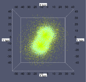
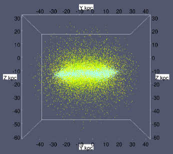
Figure 8: The collision model Orb, at the time of 5.4 Gyr, equivalent to 3.69 times the rotation period of the galaxy model. The XY view is shown on the left panel and the ZY view on the right panel. The region shown is (-50,50) kpc in the X-axis, (-50,40) in the Y-axis and (-60,30) in the Z-axis. The colors indicate the matter components according to bulge-yellow, gas-green and disk-blue.

In this model we observe a soft approach of the galaxies. Therefore, the center of mass of each galaxy enter in orbit one with respect to the other, in such a way that many complete turns of the orbital motion are observed in the central region during the evolution time within the short interval of 5.4-5.6 Gyr. At the evolution time of 6.14 Gyr, the merging process is completed. Therefore, one only sees a single rotating dense core, see Fig. 8. This dynamic can be captured by following the gas component, as is explained in the last paragraph of Section 3.3.1.

The initial conditions of the collision model labeled Tom in Table 3 are taken from one of the collision models described by  Toomre at al. (1972). The two galaxies are placed in the XY plane very close to each other. The center of mass of one galaxy has initial velocity directed outward of the XY plane in the positive direction of the Z-axis, while the second galaxy is at rest. Consequently, we say that there is an effective impact parameter on the Y-axis, as indicated in Table 3.

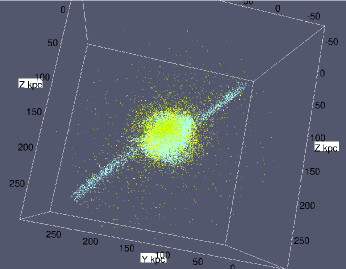
Figure 9: The collision model Tom, at the time 1.68 Gyr, equivalent to 1.12 times the rotation period of the galaxy model. In the left panel we show the XY view and in the right panel the ZY view rotated arbitrarily. The region shown is (-150,150) kpc in the X-axis, (-50,250) in the Y-axis and (-50,250) in the Z-axis. The colors indicate the matter components according to bulge-yellow, gas-green and disk-blue.

It is observed that the moving galaxy describes an arc and finally falls onto the motionless galaxy, so that the system develops an appreciable orbital movement, which causes spiral arms to develop, as can be seen in Fig. 9. It must be emphasized that these spiral arms are mainly composed of disk particles. In this model, both disks have lost their initial elongation. Most of the bulge surrounds the central part of the disk while an small fraction of the bulge particles also follows slightly the spiral arms.

The last collision model considered in this paper was labeled Rot in Table 3. This model is very similar to model Orb. In fact, in model Rot the disk planes defined in model Orb are rotated, as can be seen in the top panel of Fig. 10. The dynamic evolution shows the formation of an elongated bar, in which both the disk and the bulge take part in this rotating structure, as can be seen the middle panel of Fig. 10. Finally, a new structure is formed at the end of the evolution time as a merger remnant, such that a mass concentrated in the center is surrounded by a couple of spiral arms, which are mainly composed of both disk and the bulge particles, as can be seen in the bottom panel of Fig. 10.

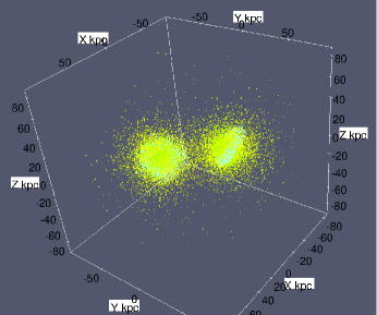
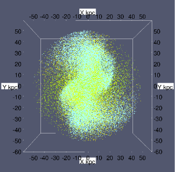
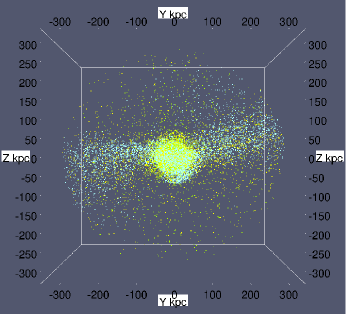
Figure 10: The collision model Rot, at the top panel we show the snapshot taken at the time 1.23 Gyr, equivalent to 0.82 times the rotation period of the galaxy model, which is seen from a view rotated arbitrarily; the region shown is (-80,80) kpc in all the axes. In the middle panel we show the XY view corresponding to 1.56 Gyr or 1.04 times the rotation period of the galaxy model. The region shown is (-50,50) kpc in the X-axis and (-50,50) in the Y-axis. It should be noticed the elongated configuration formed, in which small spiral arms are seen. Finally, in the bottom panel we show the a view rotated arbitrarily at the time 3.33 Gyr or 2.22 times the rotation period of the galaxy model. The region shown is (-300,300) in the Y-axis and (0,300) in the Z-axis. It must be noted the long spiral arms formed at the merged system. The colors indicate the matter components according to bulge-yellow, gas-green and disk-blue.

It must be emphasized that most of the collision models considered so far (with exception of the model S02b) led to the formation of a new galaxy structure, presumably with different physical properties to those observed for the original galaxy model, out of which the new structure is formed as a merger remnant. To get more details about the physical properties of these new structures, in Section 3.3 we try to characterize them by looking at (i) the dynamic behavior of the peak density of the gas component in Section 3.3.1 and (ii) the evolution of the angular momentum of the collision models in Section 3.3.2.

3.3 Dynamic characterization of the merger remnants of the collision models.

Using the visualization software pv-wave version 8, we managed to track the evolution of the gas and show short movies at the web address: https:
drive.google.com/open?id=1VUhCAZhWWnOHsh_fWKkWrhYjh8WD08I5. It must be noted that the gas shows an interesting dynamic despite the fact that it is always bounded gravitationally during the evolution time either to the central region of the galaxy model or to the merged system.

3.3.1 Time evolution of the density peak and radial density profile for the collision models

As we mentioned in Section 3.1, the gas of the galaxy model expanded very quickly to reach an equilibrium configuration, as characterized by an almost flat curve of the peak density.

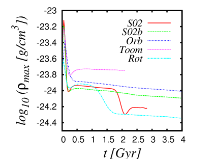
Figure 11: Time evolution of the peak density for the gas in all the collision models.

One way to quantify the effects of this gas expansion of the galaxy model on the collision models is by calculating again the time evolution of the peak density of the gas for all the collision models, as has been done in Fig. 11. In this plot, one can see that all the peak density curves rise and fall very quickly at a very small radius and then a stabilization stage follows for large radius. This indicates that the most of the gas remains bounded gravitationally to the galaxy center, while a small fraction of gas manages to escape away.

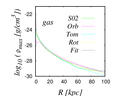
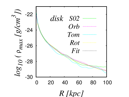
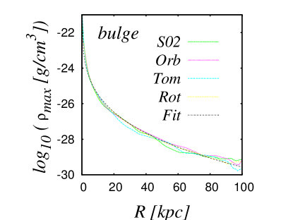
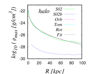
Figure 12: The radial density profile of the merger remnants formed as a result of the collision models summarized in Table 3. Fitting curves for all the models are also included.

It is in the central region of the galaxy model where the minimum of the gravitational potential well is generated by the most massive matter component, namely the dark-matter halo. Consequently, the densest gas is located in the central region of the galaxy model, and it remains rotating in the azimuthal direction while oscillating radially simultaneously.

To achieve a further characterization, we next determine the radial profile of the peak density for all the collision models. To do this, we followed the same procedure outlined in Section 3.1 about a radial partition of $n_{\rm bin}$ bins started from the center of the mass of the merger remnants up to a maximum radius of 100 kpc. As was done previously, we accounted for all the particles contained in each radial bin taking into account their matter type. We then get the mass contained in each radial bin for each matter component and thus the density at the average radius of the bin. This density versus radius calculation is plotted in four panels in Fig. 12, so that each panel corresponds to a matter component and each curve to a collision model.

It should be emphasized that due to this procedure, there are no radial density profile curves for the model SO2b in the first three panels, because there was no merging process in this model and therefore no new structure was formed. However, as the dark-matter component fills the entire volume in which the collision models take place, it is possible to determine the radial density profile for the collision model S02b in the case of the dark-matter component, which is shown in the four panels of Fig. 12.

We observed no significant difference in the curves shown in Fig. 12 with respect to the collision model, especially for large radii. In the interval 0–10 kpc, the curves for the collision model Orb show a small but noticeable difference with respect to the curves of the other collision models, as can be seen in the panel for the gas component. This behavior indicates that the process by which the mass is gathered does not make a significant difference because the mass is assembled in the new galactic structure driven by the gravitational force. Therefore, the mass is accumulated first at the central region, where the gravitational potential takes its deepest value, and later the mass is accumulated on the periphery.

To take advantage of this result, in Fig. 12 we also show the fitting curves for all of the matter components of all the collision models. This means that the free parameters of a de Vaucouleurs function have been calculated for each density profile curve shown in Fig. 12 and averaged to have only an overall fitting curve per matter component describing the behavior of the radial density profile for each matter component, irrespective of the merging geometry. More details about this fitting process are given in Appendix A.

3.3.2 The circular velocity profile and the time evolution of the angular momentum for the collision models.

Taking advantage of the radial partition described in Section 3.1, in the left-hand panel of Fig. 13 we now show the circular velocity curves of the collision models, so that the matter components are not considered separately. In addition, in the right-hand panel of Fig. 13 we show the time evolution of the magnitude of the total angular momentum for the collision models. We emphasize that both panels of Fig. 13 were calculated using all of the particles of the simulation, irrespective of the matter component type.

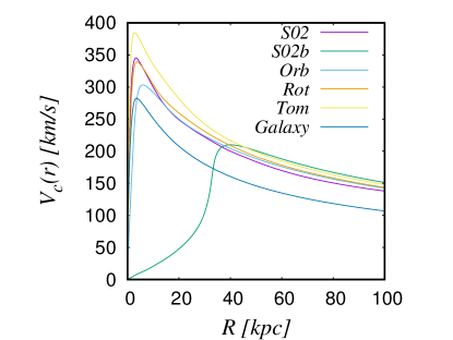
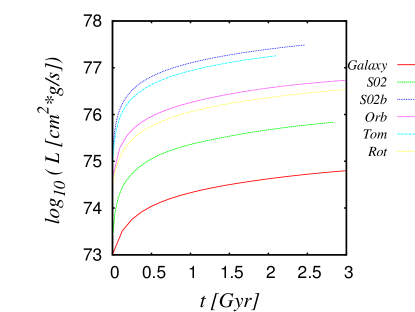
Figure 13: (left) The circular velocity for the collision models. (right) Time evolution of the magnitude of the angular momentum L. In these plots all the curves include the contribution of all the particles irrespective of the matter component type. To allow comparison with the galaxy model, the curves here labeled ”Galaxy” in these plots are taken from the curves labeled ”all” in Fig. 3.

With regard to Fig. 13, two comments are in order. First, it should be noted that the curves labeled ”Galaxy” in both panels of Fig. 13 are those that were labeled ”all” in Fig. 3, so that these curves have been repeated here for the sake of comparison between the results of the galaxy model with those shown here for the collision models. Second, as was mentioned in Section 3.3.1, for the collision model S02b, there is no a new structure in which a center of mass can be defined properly, so that there is no sense to the circular velocity curve for small radii. When the radius is large enough for the two galaxies to be included within this radius, then the circular velocity calculation does not realize that the galaxies are separated and the total galaxy mass generates the same behavior of the circular velocity curve, as the other collision models do and was observed for the galaxy model, which is that the circular velocity curves decrease as $1/\sqrt{R}$ for large $R$.

According to the right-hand panel of Fig. 13, the magnitude of the total angular momentum of the collision system increases systematically with the evolution of time. This could be due to the fact that the matter components expand radially, whence the lever arm length increases and although we expect a decrease in the magnitude of the circular velocity, the product of the two physical quantities increases.

It should be noted that all the collision models substantially increase their angular momentum with respect to that determined for the galaxy model before the collision. The higher values of angular momentum are a consequence of the orbital motion developed in the collision models, so that for the models S02b and Tom the curves are at the top of the right-hand panel of Fig. 13. The models Orb and Rot, which have followed the same 2-body pre-collision path, have an angular momentum very similar in magnitude, so their curves are at the middle of the right-hand panel of Fig. 13. The collision model S02 shows the lowest angular momentum magnitude, so that its curve is located at the bottom.

4 Discussion

The main purpose of this paper is to follow the evolution of a galaxy model, which was basically taken from the paper by Gabbasov at al. (2006). However, the widths of the disk were very different, because these authors used 0.001 kpc while we used here 1 kpc, that is, a much wider disk. We will consider a more slender galaxy model elsewhere. It must be emphasized that this difference in the galaxy models makes it difficult to compare the outputs, because a thin disk favors the growth of perturbations in the orbits of stars, which will result in the formation of a bar.

As we mentioned earlier, an important improvement of our work with respect to that of Gabbasov at al. (2006) is that we have included gas in the galaxy model. While it is true that the mass fraction of the gas is very small with respect to the fractions of the other matter components, the gas dynamics observed in Section 3.3.1 are interesting and very important to be followed from the point of view of star formation. For example,  Springel and Hernquist (2005) found that when the gas fraction is small, the resulting merger remnant usually resembles an elliptical galaxy; while if the gas fraction is high enough, then other structures can be formed.

We observed that the gas component, initially located in a ring, is moved quickly to the center of the galaxy model. Consequently, the peak density of the gas increased significantly. Shortly after, the gas is expanded up to an equilibrium radius, which is indicated by the strong decrease of the peak density determined in the left-hand panel of Fig. 5. From this moment, most of the gas evolves tied to the galaxy center while a small fraction of it managed to escape away, as is indicated by the smooth decrease of the curve shown in this panel for large evolution times.

As we mentioned in Section 3.2, the galaxy model at the evolution time $t=0$, was used in all of the collision models. Therefore, the initial gas behavior of the galaxy model was observed to happen also in the collision models, as can be noticed by comparing the magnitude of the density peak observed for the galaxy model in the left-hand panel of Fig. 5 with those determined for the collision models, which are plotted in Fig.11.

We next simulate some galaxy collision models in order to determine the effects on the distribution of the matter components in the new galaxy structures formed out of the merging process of the galaxy model. With respect to the paper by Luna at al. (2015), we emphasize that in this work the number of particles used to build the galaxy model increased significantly: Luna at al. (2015) use 1024-29491-245760 particles to represent the bulge, disk and halo, respectively. In this paper we use the numbers 33205-99950-533082, which are little more than the double. Gabbasov at al. (2006) presented a convergence study in the number of particles, so that the highest resolution simulation of these authors used 65536-196608-1048576 particles to represent the components of the bulge, the disk and the halo, respectively. This means that our particle numbers in this paper represent the half. Consequently, we conclude that the simulations presented in this paper have a resolution comparable to the papers that have served us as motivation.

In this paper, we have not observed the formation of long tails in the collision models considered in Section 3.2. However, when we described the results obtained in some collision models, such as Tom and Rot, we mentioned that some spiral arms have been formed. It must be emphasized that these structures can also be named tails, in the sense that they were formed in close encounters of the galaxy model, because the mutual tidal force made particles of the disk and bulge to be ejected from the central region. Thus, they can be named either tails or arms and these structures are small in length. The reason for the lack of long tails in our simulations was already explained by  Dubinski at al. (1996), so that the formation of long tails in interacting galaxies can be inhibited by the presence of a massive dark-matter halo. Later,  Springel and White (1999) demonstrated that a dark matter halo with a large enough spin parameter led to the formation of long tidal tails, otherwise, no tails are observed.

Before the log scale is taken in the right-hand panel of Fig. 5, this plot can be compared with the four panels of Fig. 12, we observed that the radial density profile in the galaxy model is very similar to that observed in new galactic structures formed after the collision process. It should be noted that the center of the merger remnants was defined as the center of mass, as was mentioned in Section 3.3.1. Starting from this center, we made the radial partition to calculate the physical properties presented in Section 3.3. The disadvantage of this procedure is that the centers of mass for the different matter components are slightly displaced. It should be mentioned that other choices for the center of the merger remnants are possible; for instance, the location of the particle with the minimum of the gravitational potential.

As was mentioned at the end of Section 3.3.2, we presented the de Vaucouleurs fitting curves for the radial density profiles shown in Fig. 12. The strategy followed was explained in detail in Appendix  A. The first point to be emphasized is that there is no need to fix $n$ at the value 4, as we did in this paper just for simplicity. Meanwhile, $n$ can be varied around 4 so that the best least squares fit must be chosen. From this value of $n$, the value of $b_{n}$ can then be obtained from the approximated formula $b_{n}=2n-0.327$, which was proposed by  Caon et al. (1993). Next, from the values of $A$ and $B$ given by the least squares method, the parameters $\rho_{e}$ and $R_{e}$ can be obtained. In principle, with this strategy, no parameter is left undetermined. However, with the procedure outlined in Appendix  A, the parameter $R_{e}$ is left undetermined. To deal with this situation, we varied the parameter $R_{e}$ within the interval (0.5,20) kpc and obtained all the fitting curves parameters $\rho_{e}$ and $b_{n}$.

We briefly mention the results of another case,  Bournaud et al. (2011) determined the best fitting parameters of a Sérsic function for the radial profile of the surface density for a set of compact spheroids, which were the outcome of a set of high-redshift galaxy merger simulations with high fractions of turbulent and clumpy gas: the average values found were $n=3.4$ and $R_{1/2}=4$ kpc.  Ferrarese (2006) reported the isophotal parameters and the surface brightness profiles of 100 galaxies in the Virgo Cluster, and found that the surface brightness profiles are well described by a Sérsic function. In addition,  Kormendy at al. (2009) also reported the values of the Sérsic parameters for many elliptical and spheroidal galaxies also in the Virgo cluster.

The second point that deserves attention is the use we made of the de Vaucouleurs function to describe directly a radial density profile. In fact,  Mellier and Mathez (1987) proposed a density function with the form $\rho(R)=\rho_{e}\left(\frac{R}{R_{e}}\right)^{\beta}\exp\left(\frac{R}{R_{e}}\right)^{\alpha}$, which was obtained as a deprojection of the de Vaucouleurs $\left(\frac{R}{R_{e}}\right)^{1/4}$ law. In this density function, $\alpha$ and $\beta$ are free parameters in addition to $\rho_{e}$ and $R_{e}$. It should be emphasized that the observables of a galaxy are line-of-sight projections of the corresponding three-dimensional physical quantities. In the general case, the projected quantity is related to the three-dimensional quantity by an integration along the line-of-sight spatial coordinate.

In this paper we adopted a functional form for $\rho(R)$ as that of the de Vaucouleurs function and then constrained its free parameters by comparing it to the calculated radial density profile shown in Fig. 12, which is already a three-dimensional quantity. As was shown in Section 3.3, the de Vaucouleurs function does an excellent fit with the radial density profiles shown in Fig. 12. The reason behind this success is that the de Vaucouleurs formula was designed to represent a central peak surrounded by a region where the variable of interest falls with the 1/4 power of the radius, just as the radial density profile does, irrespective of being a projected or three-dimensional quantity.

It should be emphasized that  Aguilar and White (1986) presented N-body simulations with an initial density profile of the de Vaucoulours form. At the final evolution time, they found that the density profile remains that of de Vaucoulours but with other parameters. This statement can be said in other terms, such as de Vaucouleurs surface brightness profile appears to be invariant under galaxy harassment. In this sense, it can then be considered that our paper confirms part of this result; as we mentioned earlier, the merger remnants manage to adopt a radial density profile of the de Vaucoulours form, irrespective of the pre-collision trajectory. It must be emphasized that of galaxy model used much more particles and matter components than the galaxy model of  Aguilar and White (1986) because they used 3000 particles in their galaxy collision models.

One last comment about some important physical elements of the gas that are missing in this paper, for instance  Springel (2000) presented simulations of interacting disk galaxies including star formation and feedback, where the gas is able to cool radiatively and to form collisionless stars. There is an extensive literature devoted to the study of galaxy formation and evolution by hydrodynamical simulations, some of which include this kind of complicated gas physics.

Many efforts have been made to date to incorporate star formation and feedback in simulations of galaxy formation and evolution, see for instance, Springel and Hernquist (2003). It has proven to be a difficult problem to be managed, as many recipes have been introduced and tested during many years, see for instance, Stinson et al. (2006). We have not even attempted to consider this complicated problem, which is beyond the scope of this paper, since our interest at the moment is only to put the gas on a consistent basis in a general model of a galaxy. However, we would like to comment about the importance of the lack these gas physics on simulations of galaxy collisions, like the ones presented in this paper.

As we have seen, the simulations show that the gas moves rapidly towards the central region of the dark-matter halo and therefore, the gas density increases. At some point, it will be very important to model the transformation of gas into stars. As expected, this transformation will modify the dynamics of all the matter components in the galaxy model. In addition, many simulations have demonstrated that galaxy collisions in general augment the star formation rate, from low levels (a few times the star formation rate detected for the isolated galaxy model) to high values (20-60 times the isolated galaxy case), see for instance Mateo at al. (2007). In this case, the amount of gas available will be reduced after the collision, so the curves for the radial density profile are expected to be different with respect to the isolated galaxy model when star formation be included somehow.

5 Consistency of our simulations with regard to other papers

In this Section we will try to establish the consistency of the simulations presented in this paper by comparing their results with other simulations, with observations and with virtual observations.

5.1 Comparison with other simulations

Barnes and Hernquist (1996) determined the radial density profile of their collision models and found a set of curves falling systematically for the remnant’s innermost region. It should be emphasized that in this paper we also found a similar behavior but we extend the radius up to 100 kpc from the remnant’s center.

For this reason, we claim that in the present paper we also observe this redistribution of gas to the central region and show that the gas is linked to the central region during almost all the evolution time even in cases in which a collision with another galaxy occurs. We did not observe the well defined spiral pattern of the gas in our galaxy model, as was observed by Barnes and Hernquist (1996). It should be mentioned that this spiral pattern is a transitional stage that ends quickly. We believe that this failure is due to the lack of radiative cooling in the gas component.

In addition, Hernquist and Mihos (1995) determined the time evolution of the total angular momentum of the galaxy components in their satellite merger model, and found that when the primary galaxy model includes a bulge, then the curves grow systematically. Meanwhile, the curves for the gas component fall systematically. Because the magnitude of the latter curves are quite smaller than that of the former curves, 0.03 versus 0.25 as can be appreciated in their Fig. 8, we conclude that the general behavior of the total angular momentum, when all the components are included together, should be similar to the curves shown in Fig.13 of the present paper, that is, growing systematically with the evolution time.

On the other hand, Mihos and Hernquist (1996) showed that the geometry of the orbits of the approaching galaxies does not seem to be important in the determination of the resulting dynamics of the gas. It seems to be more important the internal structure of the galaxies, for instance, the presence or absence of a bulge in the galaxy model and its physical properties. Although using only a very limited collection of approaching orbits, in the present paper we confirm this result of Mihos and Hernquist (1996), as we mentioned at the end of the Section 4, where we connect our results with those of the paper by Aguilar and White (1986).

5.2 Comparison with observations

All of the simulations reported in the papers mentioned above in Section 5.1, contributed with different elements to support the idea of the formation of elliptical galaxies by means of collisions between spiral galaxies. As Barnes and Hernquist (1996) mentioned, it happens that centrally concentrated gas systems, like the ones observed in those simulations, have been detected by means of CO interferometer observations of galaxies, for instance Arp 220, see Scolville et al. (1986) and NGC 520, see Sanders et al. (1988), among others.

We believe that the present paper reaffirms this idea, as the collision remnants seen in Figs. 8, 9 and 10 seem to be spheroidal systems supported by rotation, likely resembling the kind of systems usually classified as normal elliptical E, lenticular galaxies of the type SO, see Kormendy and Djorgovski (1989), as the size and mass of our merger remnants are around 100 kpc of radius and the total mass contained up to this radius is around 3$\times 10^{11}\,M_{\odot}$, in which all the mass components have been included.

On the other hand, by combining new surface photometry with published data, Kormendy at al. (2009) constructed composite brightness profiles over large radius ranges of all known elliptical galaxies in the Virgo cluster. It must be noted that Kormendy at al. (2009) took a conclusion (see their Section 7.2), which seems to generalize and at the same time provides some observational support to the idea described at the end of Section4 of this paper, that is, the idea that the de Vaucouleurs profile curve fits well all of the resulting merger remnants of the galaxy collisions considered in this paper, irrespective of the collision geometry.

Let us now quote that conclusion in Kormendy at al. (2009) own words: ”One of the main conclusions of this paper is that Sérsic functions fit the main parts of the profiles of both elliptical and spheroidal galaxies astonishingly well over large ranges in surface brightness. For most galaxies, the Sérsic fits accurately describe the major-axis profiles over radius ranges that include ∼ 93–99 percent of the light of the galaxies (see Figure 41). At small r, all profiles deviate suddenly and systematically from the best fits.” Later, in their Section 9.2, Kormendy at al. (2009) continued in this way: ”This result is remarkable because there is no astrophysical basis for the Sérsic function. We know no reason why violent relaxation, dissipation, and star formation should conspire-surely in different ways in different galaxies-to produce so simple and general a density profile.”

5.3 Comparison with virtual observations

The Illustris cosmological hydrodynamic simulation, which is described by Vogelsberger et al. (2014), has successfully reproduced the distributions of galaxies in clusters, so that both spirals and elliptical galaxies can be distinguished morphologically for the first time, as far as we know.

By using a suite of simulations based on the Illustris simulation, Taylor et al. (2016) determined the mass profile of a dark-matter halo in which there is embedded a galaxy with a mass comparable to the Milky Way’s mass. In the left panel of their Fig.2 they show the circular velocity curves for the chosen mass systems (consider only the curves labeled as ”D12”). The curves grow rapidly for small radius, until a peak circular velocity is reached, from which the curve falls smoothly as the radius increases. It must be emphasized that the shape of these curves is very similar to those shown in the left panel of Fig.3, calculated in the present paper to characterize the galaxy model.

When they include all their matter components (dark-matter, gas and stars) in the calculation of the circular velocity, their peak velocity is a little below 200 km/s; in our case, when we included all the four matter components, we obtained a peak value around 270 km/s, see the curve labeled as ”all” in the left panel of Fig.3. The peak velocity of the curve for the dark-matter halo is a little up 200 km/s, see the curve labeled as ”halo” again in the left panel of Fig.3.

When they separate their mass components in their calculation of the circular velocity, see the right panel of their Fig.2, they obtained for the gas a curve around 50 km/s. In our case, our corresponding curve for the gas component is around 30 km/s.

We can compare their circular velocity curves with the ones we obtained for the merger remnants, which are shown in the left panel of Fig.13. Because the mass assembled in the remnants is a bit more massive than the galaxy model, all the curves are higher in magnitude than those of Taylor et al. (2016). The peak circular velocity of the curves shown in Fig.13 occurs for a radius around 10 kpc, while that radius of Taylor et al. (2016) for their curves is around 20 kpc.

As the radial profile of the circular velocity is a good indicator of the mass distribution of a system, then we can conclude, on the basis of the previous comparison, that we have roughly modeled a system of a similar mass and size of those chosen for Taylor et al. (2016) to model the Milky Way galaxy.

6 Concluding Remarks

In this paper we implemented a galaxy model that proved to be stable over a long evolution time. As an improvement over the papers of  Gabbasov at al. (2006) and  Luna at al. (2015), on which this work is based, here we included a gas component.

Using this galaxy model, we then explored several collision models of equal-mass galaxies to study the effects of different interaction scenarios on the dynamic of the matter components of the new structures formed after such merging process. As expected, the interaction between galaxies produce notable changes in the galaxies participating and in their physical properties. We here focused specifically on the density profile. Some of the conclusions to be emphasized from the models calculated here follow:

1. The galaxy model has proved to be stable (in the sense that it has reached a state of dynamic equilibrium) up to an evolution time of 14 Gyr.

2. Most of the gas of the galaxy model evolved strongly tied to the galaxy center, while a small fraction of it managed to escape away with the evolution of time.

3. The collision models considered in this paper are not intense enough to significantly eject the gas from the central mass distribution of the galaxy model.

4. The gas is gravitationally bounded to the center of each of the galaxies even during the process of collision.

5. The gas shows an interesting dynamics, despite the fact that it is always bounded gravitationally to the central region of the newly formed system.

6. It should be noted that all the collision models substantially increase their angular momentum with respect to that of the individual galaxy before the collision.

7. The dynamic variables studied in Section 3.3 (e.g. peak density, density profile and angular momentum) do not capture the moment at which the merging process of the two galaxies takes place.

8. It seems to be that the radial density profile does not make any difference with respect to the collision process that gather the mass together. Therefore it is possible to obtain an overall general de Vaucouleurs curve to describe the general behavior of the radial density profile of the merger remnants. The fitting parameters of the de Vaucouleurs curve are describe in Table 4 and in Fig. 14.

9. The four-parameters formula considered in Appendix B also fits well in general the radial density profile for radii within 10-20 kpc. But, for some collision models, like the Orb y Tom, there are considerable deviations for very small radii.

Appendix A The de Vaucouleurs fitting curves

Let us thus adapt the de Vaucouleurs function to describe the radial profile of the peak density calculated in Section 3.3.1, which in this paper will be considered to be given as

$$\rho(R)=\rho_{e}\,\exp\left\{-b_{e}\left[\left(\frac{R}{R_{e}}\right)^{1/4}-1\right]\right\}$$ (1)

In the case of the surface brightness $I$, $R_{e}$ is known as the effective radius or half-light radius, because this indicates the radius within which the brightness of the elliptical galaxy includes half the light of the image. For this paper, $\rho_{e}$, $b_{e}$ and $R_{e}$ are free parameters of Eq.1, which must be determined.

By taking the natural logarithm on both sides of Eq. 1 and defining $x=R^{1/4}$, $x_{e}=R_{e}^{1/4}$, $y=\log{\rho}$ and $y_{e}=\log{\rho_{e}}$ we get

$$y=A+B\,x$$ (2)

where $A$ and $B$ are parameters to be determined by the least squares method applied to the data shown in the plots of Fig. 12, where $y$ and $x$ take the values $y_{i}$ and $x_{i}$ with $i=1..n_{\rm bin}$, as was done in Section 3.1, where the radial partition was described. These parameters are related to the de Vaucouleurs parameters by means of

$$\begin{array}[]{l}A=b_{e}+y_{e}\vspace{0.1 cm}\\ B=-\frac{b_{e}}{x_{e}}\end{array}$$ (3)

so that there are three free parameters in the right-hand side of Eq. 3, while the least squares method gives us only two parameters in the left-hand side of Eq. 3. To solve this issue, we consider the following strategy, which is obviously not unique, see the end of Section 4. We make a partition in the radial parameter $R_{e}$ so that we scan a relevant interval, for example from 0.5 to 20 kpc. Then having the values of $A$ and $B$ by using the procedures of Press et al. (1992) and fixing the value for $R_{e}$, we then obtain the corresponding values of de Vaucouleurs parameters $b_{e}$ and $\rho_{e}$ by means of

$$\begin{array}[]{l}b_{e}=-x_{e}\,B\vspace{0.1 cm}\\ y_{e}=A-b\end{array}$$ (4)

It is interesting to mention that this strategy led us to a unique curve from all the curves for each $R_{e}$. This means that the increment in the value of the parameter $R_{e}$ produces a change in the values of the parameters $b_{e}$ and $\rho_{e}$, so that the three parameters produce the same curve by means of Eq.1, for every value of $R_{e}$ within the scanned interval.

Table 4: The averaged parameters of the de Vaucouleurs fitting curves for the radial density profile. The parameter $R_{e}=0.5$ kpc.

matter component	$b_{e}$	$\rho_{e}$
gas	4.97	2.767 $\,\times 10^{-24}$
disk	6.03	1.006 $\,\times 10^{-22}$
bulge	5.85	1.925 $\,\times 10^{-23}$
halo	4.75	1.108 $\,\times 10^{-22}$

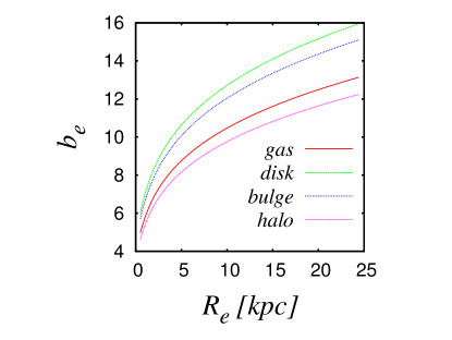
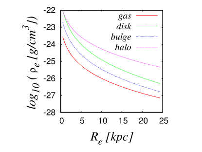
Figure 14: Averaged values of the de Vaucouleurs parameters as a function of the value of the parameter $R_{e}$, (left) $b_{e}$ and (right) $\rho_{e}$.

Finally, given that there are four matter components and four collision models, once we have the fitting curve for every model and matter component, we then take the averaged values of the parameters $b_{e}$ and $\rho_{e}$ for a fixed value of $R_{e}$, so that the resulting averaged fitting curves have been plotted in each panel of Fig. 12. It should be noticed that these averaged values for the de Vaucouleurs parameters $b_{e}$ and $\rho_{e}$ are reported in Table 4.

With the procedure followed in this Appendix A, the parameter $R_{e}$ is left undetermined. To alleviate this issue, in Fig. 14 we show the values of $b_{e}$ and $\rho_{e}$ obtained as a function of $R_{e}$.

Appendix B A four-parameters fitting curves

The objective of this Appendix B is twofold. First, to complement the curves of the radial density profile shown in Section 3.3.1, which were constructed by using a radial partition up to a maximum radius of 100 kpc, so that now we shorten this radial range up to 40 kpc, to show the gas distribution of the innermost region of the merger remnants with more detail. Second, to complement the results of Appendix A, where a de Vaucouleurs function was proposed to describe the radial density profile, so that now we test another radial formula which has given good results as a fitting model, as we explain below.

Recently, Wang et al. (2014) focused on understanding the radial distribution of the gas in a sample of spiral galaxies, showed that there is a mathematical function that works well as a fitting model for the radial profiles of the HI surface density for the 42 galaxies, which are part of a sample of galaxies of the Bluedisk project, see Wang et al. (2013). The formula is shown in Eq.1 of Wang et al. (2014) and we repeat it here for the reader’s convenience:

$$\Sigma(x)=\frac{I_{1}\,\exp\left(-x/r_{s}\right)}{1+I_{2}\,\exp\left(-x/r_{c}\right)}$$ (5)

where $\Sigma$ is the surface density and $I_{1}$, $r_{s}$, $I_{2}$, $r_{c}$ are free parameters to be determined by adjusting the curve to the data available. By using an ANSI C translation of the MPFIT program, see Garbow et al. (2013), we calculate the best fitting parameters to solve the least-squares problem applied to the data $\rho_{ave}(R)$ versus $R$, where $\rho_{ave}(R)$ is the average density for a thin radial shell centered around the radius $R$ with a width given by $\delta R$. The resulting curve is shown in the left panel of Fig.15. The set of parameters per each collision model is shown in Table5.

In this case, the function $\Sigma(x)$ defined in Eq. 5 has been identified directly with the mass density $\rho(R)$ and the independent variable $x$ with the radius $R$. Let us compare our results with those of Aumer and White (2013), who presented simulations of gas disk formation and evolution, so that they located gas at redshift 1.3 in some dark-matter halos chosen from a dark-matter-only simulation. The gas evolved up to a redshift zero in a zoom-in cosmological re-simulation. In the right panel of the second line of their Fig.12, they reported the surface gas density (in units of $10^{10}\,\times\,\frac{M_{\odot}}{kpc^{3}}$) versus the disk radius (in kpc), so we include in the sixth column of Table5 the values obtained for the following combination of fitting parameters: $\rho_{ave}^{\Sigma}(0)=\frac{I_{1}}{1+I_{2}}$, which corresponds to the value of the fitting curve at $R=0$, see Eq.5. Aumer and White (2013) reported a value of $10^{-1}$ at $R=0$, which is very high compared to our values, which are in the range from $1.2\,\times 10^{-3}$ to $6.95\,\times 10^{-4}$.

In order to compare with the paper of Wang et al. (2014), we calculate an approximate surface density profile based on the procedure already explained above to obtain the radial density profile (see also Sections 3.1 and 3.3.1). As we mentioned, we made a radial partition of the spherical galaxy in terms of spherical shells centered on a radius $R_{i}$, so that the number and type of the particles contained in each radial shell was accounted for and we simply divide it by the surface area of the shell at the radius, which is $4\pi R_{i}^{2}$ on average. We present our results in a log-log plot and changed the units of the surface density to make comparison easier.

It must be noted that we have applied the fitting process on the log-log data directly to determine the parameters of the best fitting curve. In this case, we have identified the $\Sigma(x)$ defined in Eq. 5 with $\log(\Sigma_{ave})$ and the $x$ with $\log(R)$. The fitting curve is shown in the right panel of Fig.15 and the parameters are reported in Table 6.

The average values of the parameters $r_{s}$ and $r_{c}$ for the 43 galaxies reported by Wang et al. (2014) are $<r_{s}>=5.77$ kpc and $r_{c}=4.23$ kpc, while our average values obtained for the plot shown in the left panel of Fig.15 are $<r_{s}>=0.9$ kpc and $r_{c}=1.17$ kpc. While it is true that the curves of the right panel of Fig.15 show a similar shape to the curves reported by Wang et al. (2014) in their Figs. 1, 4 and 5, our curves are quite below their curves, as can be seen in the sixth column of Table 6, in which we show the expected value of our fitting curve $\Sigma_{ave}(0)$ ( now without the log scale ) at r=0. Wang et al. (2014) showed a value of the surface density at r=0 within 1 to 10, while our values are always below 1.

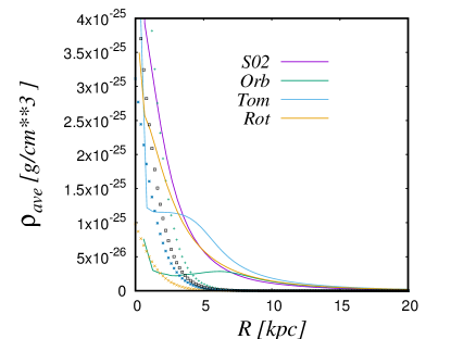
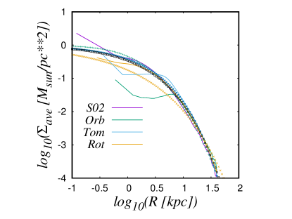
Figure 15: The radial density profile of the merger remnants (shown with lines) and the fitting curves (shown with points) for the collision models.

Table 5: Parameters of the four-parameters fitting curves shown in Eq.5 for the radial density profile.

model	$I_{1}$ [$g/cm^{3}$]	$r_{s}$ [kpc]	$I_{2}$ []	$r_{c}$ [kpc]	$\rho_{ave}^{\Sigma}(0)$[ $10^{10}\,\times\,\frac{M_{\odot}}{kpc^{3}}$]
S02	$2.01\,\times 10^{-24}$	0.948	1.34	1.13	$1.27\,\times 10^{-3}$
Orb	$2.28\,\times 10^{-25}$	0.9489	1.32	1.21	$1.45\,\times 10^{-4}$
Tom	$7.29\,\times 10^{-25}$	0.94	1.34	1.17	$4.6\,\times 10^{-4}$
Rot	$1.1\,\times 10^{-24}$	0.94	1.34	1.15	$6.95\,\times 10^{-4}$

Table 6: Parameters of the four-parameters fitting curves shown in Eq.5 applied directly to the log-log data of the radial density profile.

model	$I_{1}$ [$\log_{10}(\frac{M_{\odot}}{pc^{2}})$]	$r_{s}$ [$\log_{10}(kpc)$]	$I_{2}$ []	$r_{c}$ [$\log_{10}(kpc)$]	$\Sigma_{ave}(0)$[ $\frac{M_{\odot}}{pc^{2}}$]
S02	-0.94	-1.05	1.8	0.56	0.46
Orb	-30.89	-1	40	760	0.17
Tom	-5.5	-0.9	12.12	3.13	0.38
Rot	-7.19	-1.7	14.22	1.17	0.33

References

- Aguilar and White (1986) Aguilar, L. and White, S.D.M., 1986, The Astrophysical Journal, 307, pp.97-109.
- Aumer and White (2013) Aumer, L. and White, S.D.M., 2013, MNRAS 428, pp.1055–1076.
- Athanassoula and Bosma (2019) Athanassoula, E. and Bosma, A., 2019, Nature Astronomy, 3, pp.588-589.
- Balsara (1995) Balsara, D., 1995, J. Comput. Phys. 121, 357.