Graceful exit problem in warm inflation

Abstract

A seemingly simple question, how does warm inflation exit gracefully?, has a more complex answer than in a cold paradigm. It has been highlighted here that whether warm inflation exits gracefully depends on three independent choices: The form of the potential, the choice of the warm inflation model (i.e., on the form of its dissipative coefficient) and the regime, of weak or strong dissipation, characterizing the warm inflation dynamics. Generic conditions on slow-roll parameters and several constraints on the different model parameters required for warm inflation to exit gracefully are derived.

I Introduction

Warm inflation (WI) Berera:1995ie , a variant inflationary paradigm, where the inflaton field dissipates its energy to a thermal bath throughout inflation, has many attracting features than its counterpart, the cold inflationary paradigm. First of all, WI takes into account the interactions of the inflaton field with other particle degrees of freedom during inflation, which are in general ignored or considered negligible in a cold inflation paradigm. Due to these interactions of the inflaton field, when WI ends, it ends in a universe which has an existing thermal bath. This is unlike the case of the cold paradigm where the universe ends up in a state devoid of matter at the end of inflation, thus requiring a subsequent phase of (p)reheating. As WI smoothly ends in a radiation dominated universe, it avoids a following reheating phase — physics of which is yet not fully understood. Secondly, the dissipative effects that are intrinsic to the WI picture offers an opportunity of alleviating some of the long-lasting problems related to cold inflation. In particular, recent works on WI have shown that for sufficiently strong dissipation, sub-Planckian inflaton values are allowed during inflation Bastero-Gil:2019gao ; Kamali:2019xnt ; Das:2020xmh . This supports the current data Akrami:2018odb which prefer small field models over the large-field ones. It also leads to a lower radiation temperature that significantly alleviates and possibly solves issues related to overproduction of unwanted relics and, e.g., the gravitino problem Sanchez:2010vj ; Bartrum:2012tg . WI has also been shown (see, e.g., Ref. Bastero-Gil:2019gao ) to provide a natural solution to the so-called eta-problem plaguing some cold inflation models in the supergravity context. In addition, it has been shown that an appropriate baryon asymmetry can possibly be generated by dissipative effects alone during warm inflation BasteroGil:2011cx . This, on the other hand, yields additional observable baryon isocurvature perturbations Bastero-Gil:2014oga , which can be probed to check the consistency of WI models. Third, WI has a more enhanced scalar curvature perturbation spectrum, which yields a lesser tensor-to-scalar ratio and, thus, helps accommodate models that would otherwise be ruled out by the observations in a cold paradigm Akrami:2018odb . The monomial chaotic inflaton potentials Benetti:2016jhf ; Berera:2018tfc are one such example. Fourth, but not the least, it has been shown that the fluctuation-dissipation dynamics, which is an inherent feature of WI model realizations, can help solving the initial condition problem of plateau-like potentials and at the same time can work as a mechanism which helps localize the inflaton at the origin to trigger a period of sufficient slow-roll inflation Bastero-Gil:2016mrl .

In its initial days, WI was considered hard to be implemented through a consistent microscopic model, with the difficulty been mostly related to the problem of shielding the inflaton sector from large thermal corrections Berera:1998gx ; Yokoyama:1998ju , which would endanger the required flatness of the inflaton potential. However, this difficulty was soon overcome, first by decoupling the inflaton sector from the light radiation fields (for its model building construction, see Refs. Berera:2008ar ; BasteroGil:2012cm , while for the consistency with observations, see Ref. Bartrum:2013fia ) and, later, by using an analogous model motivated by the Higgs phenomenology, it was shown how the inflaton could be coupled directly to the light radiation fields, yet preventing any harmful large thermal corrections to the inflaton potential. This was initially shown to be possible when the inflaton was directly coupled to light fermion fields Bastero-Gil:2016qru , a model that was named Warm Little Inflaton (WLI) model, and more recently through a variant of the WLI, where the inflaton was coupled directly to light scalar bosonic fields Bastero-Gil:2019gao . We will call the latter the variant of Warm Little Inflaton (VWLI) model. Another model with similar features to the WLI and VWLI, but motivated by the physics of axions and natural inflation has been named the Minimal Warm Inflation (MWI) model Berghaus:2019whh . One thing which is common to all these models is that the dissipation coefficient typical of the WI dynamics can all be expressed through a simple functional form that is dependent on the temperature $T$ of the thermal bath and the amplitude $\phi$ of the inflaton field. The simplest functional form assumed in most phenomenological studies involving WI involves a dissipation coefficient $\Upsilon$ given by

$$\Upsilon(\phi,T)=C_{\Upsilon}\,T^{p}\phi^{c}M^{1-p-c},$$ (1)

where $C_{\Upsilon}$ is a dimensionless constant (that carries the details of the microscopic model used to derive the dissipation coefficient, e.g., the different coupling constants of the model — see, for example, Ref. BasteroGil:2010pb for different $C_{\Upsilon}$ expected for the dissipation coefficient in WI, depending on the interactions involved and regime of parameters). The numerical powers given by $c$ and $p$, can be either positive or negative numbers and $M$ is some appropriate mass scale, such that the dimensionality of the dissipation coefficient in Eq. (1) is preserved, $[\Upsilon]=[{\rm energy}]$.

WI has also more recently regained attention in the literature in the context of the so-called Swampland Conjectures Obied:2018sgi ; Garg:2018reu ; Ooguri:2018wrx ; Kinney:2018nny . The Swampland Conjectures have been formulated as conditions that an effective field theory should satisfy in order to accommodate an ultraviolet complete field theory within a String landscape. For instance, in terms of the standard slow-roll coefficients,

$$\epsilon_{V}=\frac{M_{\rm Pl}^{2}}{2}\left(\frac{V^{\prime}}{V}\right)^{2},\quad\eta_{V}=M_{\rm Pl}^{2}\frac{V^{\prime\prime}}{V},$$ (2)

with $M_{\rm Pl}\equiv 1/\sqrt{8\pi G}\simeq 2.4\times 10^{18}$GeV is the reduced Planck mass, the de Sitter conjecture, requires either $\epsilon_{V}>\mathcal{O}(1)$ or $\eta_{V}<-\mathcal{O}(1)$ Garg:2018reu ; Ooguri:2018wrx . Thus, the de Sitter swampland conjecture alone tends to overrule the generic conditions for inflation, which requires $\epsilon_{V}\ll 1$, $\eta_{V}\ll 1$ instead. This makes it difficult for the usual cold inflation to be realized in the landscape of a string theory. As WI modifies the slow-roll conditions, which are now expressed as $\epsilon_{V}\ll 1+Q$ and $\eta_{V}\ll 1+Q$, where the dimensionless quantity $Q\equiv\Upsilon/(3H)$ can be larger than 1, this paradigm can much easily accommodate the Swampland Conjectures. This was first noted in Ref. Das:2018hqy , and later, quite a few discussions along the same line have followed Motaharfar:2018zyb ; Das:2018rpg ; Bastero-Gil:2018yen ; Bastero-Gil:2019gao ; Kamali:2019xnt ; Das:2019hto ; Berera:2019zdd ; Goswami:2019ehb ; Brandenberger:2020oav ; Berera:2020dvn ; Das:2020xmh .

Aside its many attractive features, ending inflation in WI scenario is, in a sense, a more complex process than in the cold paradigm, and this is the main aim of this article — analyze how (and whether) WI gracefully exits. In a generic cold paradigm, inflation takes place when $\epsilon_{H}\sim\epsilon_{V}\ll 1$ and terminates when $\epsilon_{V}$ becomes of the order 1 (here $\epsilon_{H}$ and $\epsilon_{V}$ are the Hubble and potential slow-roll parameters in their conventional forms, respectively). Hence, the cold inflation paradigm is always in need of appropriate forms of potentials which yield growing slow-roll parameters ($\epsilon_{V}$) in time (or with number of $e$-foldings $N$). On the other hand, in the WI paradigm, inflation ends when $\epsilon_{V}\sim 1+Q$. This comes from the fact that, in WI, the Hubble slow-roll parameter becomes $\epsilon_{H}\sim\epsilon_{V}/(1+Q)$ Berera:2008ar ; BasteroGil:2009ec , and thus inflation ends when the Hubble slow-roll parameter becomes of the order unity ($\epsilon_{H}\sim 1$) or, equivalently, the potential slow-roll parameter, $\epsilon_{V}$, becomes of the order $1+Q$. However, $Q$, in general, evolves during inflation, as well as the potential slow-roll parameter $\epsilon_{V}$. Both can increase, decrease or even can remain constant depending on the form of the potential, the region (strong ($Q\gg 1$) or weak ($Q\ll 1$)) in which WI is taking place and also on the form of the dissipative coefficient (i.e., on the choice of the WI model). Note also that the end of the slow-roll inflationary phase in WI is also related by the fact that radiation can smoothly overtake the inflaton potential energy density at end. Putting in these terms, the problem of graceful exit can also be expressed by the fact that even though radiation is being produced as a consequence of dissipation, it might never overtake the inflaton energy density. Without an efficient mechanism to shut down dissipation, inflation can then prolong to asymptotic large times, with both radiation and inflaton energy densities decreasing but without radiation becoming dominant. We will give explict examples where this can happen. Hence, graceful exit is a more complex issue in WI than it is in cold inflation.

To our knowledge, a systematic study of the relevant parameter space corresponding to typical WI models that fully leads to a graceful exit is still lacking in the literature. The main objective of this work is exactly to fill this important gap. Besides of investigating this issue, we also analyze, as a consequence of our study, those generic WI potential and dissipation model parameters region of space where the dissipation ratio can grow or decrease. This is of particular importance for example in several model buildings in WI.

In the next section, Section II, we introduce the problem in more details. Then, in Section III, we discuss our results when considering different forms of dissipation coefficients typically considered in many WI studies and also with different large classes of inflaton primordial potentials. Potential applications of our results are discussed in Section IV. Finally, in Section V, we give our conclusions and final remarks.

II Setting up the problem

To look into the matter more closely, we need to first look at the basic background dynamics of WI. In the leading adiabatic approximation, the dynamics of the inflaton field in WI has an extra friction term arising due to dissipation,

$$\ddot{\phi}+3H(1+Q)\dot{\phi}=-V^{\prime}(\phi),$$ (3)

while the dynamics of the radiation energy density $\rho_{R}$ is given by

$$\dot{\rho}_{R}+4H\rho_{R}=3HQ\dot{\phi}^{2},$$ (4)

where dots denote temporal derivatives, $H$ is the Hubble parameter,

$$H^{2}\equiv\left(\frac{\dot{a}}{a}\right)^{2}=\frac{1}{3M_{\rm Pl}^{2}}\left(\frac{\dot{\phi}^{2}}{2}+V+\rho_{R}\right),$$ (5)

where $a$ is the scale factor and the dimensionless quantity $Q$ is defined as,

$$Q\equiv\frac{\Upsilon}{3H},$$ (6)

$\Upsilon$ being the dissipation coefficient. In general, $\Upsilon$ can be a function of both $\phi$ and $T$. Different forms of dissipative coefficients, derivable from nonequilibrium quantum field theory methods, have been studied extensively in the literature Berera:1998gx ; Berera:2008ar ; BasteroGil:2009ec ; Zhang:2009ge ; BasteroGil:2010pb ; BasteroGil:2012cm .

The graceful exit problem can be simply formulated as follows. Inflation takes place in the WI scenario when $\epsilon_{V}<1+Q$ and ends when $\epsilon_{V}\sim 1+Q$. Therefore, if $Q$ increases with the number of $e$-foldings, then $\epsilon_{V}$ has to increase faster than $Q$ in order to end inflation. On the other hand, when $Q$ decreases, inflation naturally ends if $\epsilon_{V}$ increases with the number of $e$-foldings or just remains as a constant. Otherwise, $\epsilon_{V}$ has to decrease with a slower rate than $Q$ in order to end inflation. To put it simply, we have that

$$\epsilon_{H}\equiv-\frac{\dot{H}}{H^{2}}\simeq\epsilon_{wi}\equiv\frac{\epsilon_{V}}{1+Q},$$ (7)

which implies that inflation takes place when $\epsilon_{wi}<1$ and ends when $\epsilon_{wi}\sim 1$. This shows that $\epsilon_{wi}$ has to grow with the number of $e$-foldings $N$ in order to end inflation, yielding the condition

$$\frac{d\ln\epsilon_{V}}{dN}>\frac{Q}{(1+Q)}\frac{d\ln Q}{dN},$$ (8)

where $dN=Hdt$. It is now quite apparent from Eq. (8) that if $Q$ is an increasing function of $N$, then $\epsilon_{V}$ has to increase faster than that (noticing the fact that both $\epsilon_{V}$ and $1+Q$ are positive quantities). On the other hand, when $Q$ decreases with $N$, then either $\epsilon_{V}$ can grow at any rate or may not evolve at all. But if $\epsilon_{V}$ decreases too, then it has to decrease slower than $Q$. All these conditions have been stated in the previous paragraph. It is also clear from Eq. (8) that when $Q$ does not evolve with $e$-foldings, $\epsilon_{V}$ can grow at any rate, just like in the cold inflation scenario, in order to end inflation.

It is to note here that in cold inflation, inflation generally does not end when the inflaton field gets trapped into some false vacuum. However, that is not necessarily the only reason behind a non-graceful exit in the case of WI. We can see from the above discussion that, mostly, inflation does not end in cases in Warm inflation when $Q$ grows faster than $\epsilon_{V}$. As the presence of $Q$ in the equation of motion of the inflaton field acts like an extra frictional term over the one for the expansion term, an increasing $Q$ will eventually lead to an overdamped equation of motion for the inflaton field. That means, that the inflaton field will only reach the minimum of the potential in asymptotic time, resulting in a scenario of never-ending WI.

We will now derive the general conditions under which WI undergoes a graceful exit. In order to do so, we assume a generic parametrization for the dissipation coefficient $\Upsilon$ as a function of $\phi$ and the temperature $T$ as given by Eq. (1). The parametrization given by Eq. (1) covers a large class of WI models that have been studied before in the literature. For instance, early dissipation coefficient derived in Refs. Gleiser:1993ea ; Berera:1998gx , corresponds to $p=-1,c=2$, the one derived in Refs. Berera:2008ar ; BasteroGil:2012cm corresponds to $p=3,c=-2$. The dissipative coefficient, $\Upsilon$, in WLI model varies linearly with the temperature $T$, as $\Upsilon(T)\propto T$ Bastero-Gil:2016qru , corresponding to $p=1,c=0$ in Eq. (1), whereas in MWI model it varies with a cubic power of $T$, $\Upsilon(T)\propto T^{3}$ Berghaus:2019whh , where $p=3,c=0$. However, the temperature dependence of $\Upsilon$ in VWLI model is more complex, given by Bastero-Gil:2019gao

$$\Upsilon\simeq{C}{M^{2}T^{2}\over m^{3}(T)}\left[1+{1\over\sqrt{2\pi}}\left({m(T)\over T}\right)^{3/2}\right]e^{-m(T)/T},$$ (9)

where $M$ is a mass scale of the model, $m^{2}(T)=m_{0}^{2}+\alpha^{2}T^{2}$ is the thermal mass for the light scalars coupled to the inflaton in the model of VWLI, with $m_{0}$ the vacuum mass of those light scalars and $\alpha$ is a coupling constant (actually, a combination of coupling constants appearing in the Lagrangian density of the model). Considering the leading behavior when the effective mass is dominated by its thermal part, $m(T)\sim\alpha T$, the dissipation coefficient (9) varies as $\Upsilon(T)\propto T^{-1}$, realizing the case with $p=-1,c=0$ in Eq. (1). On the other hand, as the temperature of the thermal bath drops and the vacuum term $m_{0}$ in $m(T)$ starts no longer to be negligible, it effectively would correspond to values of $p>-1$, with a limiting case of $p=2$ when $m_{0}\gg\alpha T$ (with an exponentially suppressed dissipation). The parametrization assumed here for the dissipation coefficient, Eq. (1), also covers other particular forms for the dissipation coefficient and used in earlier phenomenological studies, like the case $p=0,\,c=0$ (a constant dissipation coefficient form), which can be considered as a particular case that can emerge for some specific dynamical regimes in the more general dissipation coefficient Eq. (9). Also, cases with $p=0$ (but with particular powers of the inflaton field), e.g., such that $\Upsilon\propto H$, can mimic many previous phenomenological studies of WI dynamics, since it leads strictly to a constant dissipation ratio $Q=\Upsilon/(3H)$. Such a form leading to a constant dissipation ratio is particularly useful for deriving analytical results in WI and has been employed by many authors before exactly because of that (see also, e.g., Refs. Zhang:2009ge ; Herrera:2013rra ; Herrera:2014mca ; Visinelli:2016rhn ; Jawad:2017rkq ; Jawad:2017gwa for different applications in WI using a generic form for the dissipation coefficient).

In the analysis that follows now, we will also employ the slow-roll approximated dynamical equations of WI, which follow directly from Eqs. (3), (4) and (5),

$$\!\!\!\!\!\!\!3H(1+Q)\dot{\phi}\simeq-V^{\prime},\quad\rho_{R}\simeq\frac{3Q\dot{\phi}^{2}}{4},\quad 3H^{2}\simeq\frac{V}{M_{\rm Pl}^{2}}.$$ (10)

It is important to note here that the slow-roll conditions in WI do not imply the slow-roll parameters $\epsilon_{V}$ and $\eta_{V}$ to be smaller than unity. One can have these slow-roll parameters to be large, while still maintaining the required conditions for inflation, e.g., $\epsilon_{H}\ll 1$, provided that we have $Q\gg 1$, as one can see from Eq. (7). From the previous equations, one can find out, after simple manipulations, that $Q$ is related to the form of the chosen potential as

$$(1+Q)^{2p}Q^{4-p} = \frac{M_{\rm Pl}^{2p+4}C_{\Upsilon}^{4}M^{4(1-p-c)}}{2^{2p}3^{2}\,C_{R}^{p}}\frac{V^{\prime 2p}}{V^{p+2}}\phi^{4c}$$ (11)

$$\equiv \tilde{C}\frac{V^{\prime 2p}}{V^{p+2}}\phi^{4c},$$

where $C_{R}$ is the Stefan-Boltzmann factor relating the radiation energy density to the temperature, $\rho_{R}=C_{R}T^{4}$. This allows us to determine how $Q$ evolves during WI,

$$C_{Q}\frac{d\ln Q}{dN}=(2p+4)\,\epsilon_{V}-2p\,\eta_{V}-4c\,\kappa_{V},$$ (12)

where

$$C_{Q}\equiv 4-p+(4+p)Q.$$ (13)

In Eq. (12), besides the standard slow-roll coefficients (2), we have also defined

$$\kappa_{V}\equiv M_{\rm Pl}^{2}\frac{V^{\prime}}{\phi V}.$$ (14)

We also note that $C_{Q}$ in Eq. (13) is a positive quantity, otherwise $C_{Q}<0$ leads to a condition $Q<(p-4)/(p+4)$. As, so far, all the viable models of WI have temperature dependent dissipative coefficients with $-4<p<4$, which is required from the stability studies of the WI dynamics Moss:2008yb ; delCampo:2010by ; BasteroGil:2012zr . Thus, we will treat $C_{Q}$ as a positive quantity henceforth. On the other hand, depending on the form of the inflaton potential, $\epsilon_{V}$ evolves during WI as

$$\frac{d\ln\epsilon_{V}}{dN}=\frac{4\epsilon_{V}-2\eta_{V}}{1+Q}.$$ (15)

Eqs. (8), (12) and (15), along with the forms of the primordial inflaton potential and dissipation coefficient in WI, give all we need for our analysis.

III Determining the region of parameters for graceful exit in WI

We will now discuss how WI makes a graceful exit on a case-by-case basis.

III.1 Increasing $\epsilon_{V}$

We see from Eq. (15) that $\epsilon_{V}$ increases for potentials with $4\epsilon_{V}-2\eta_{V}>0$. This encompasses a large class of inflaton potentials commonly used in inflationary theories, such as the whole range of monomial chaotic potentials,

$$V(\phi)=\frac{V_{0}}{n}\left(\frac{\phi}{M_{\rm Pl}}\right)^{n},$$ (16)

and the concave potentials, which are presently preferred by the data and for which $\eta_{V}$ is negative Akrami:2018odb . Though the conventional monomial potentials, namely the quadratic and the quartic, are not in good agreement with the data in a cold inflationary scenario Akrami:2018odb , they match with the observations very well in a WI setup as they produce less tensor-to-scalar ratio in such cases Benetti:2016jhf ; Berera:2018tfc ; Bartrum:2013fia . Thus, monomial potentials are still of importance as long as one is dealing with WI.

III.1.1 Positive $\eta_{V}$

First, let us consider the potentials for which $\eta_{V}$ is positive, e.g., the monomial potentials, Eq. (16), which we will take as an explicit example. Here, $\epsilon_{V}$ increases when

$$\frac{\epsilon_{V}}{\eta_{V}}>\frac{1}{2}.$$ (17)

In such a case, $Q$ grows with $N$ if

$$n>\frac{2p-4c}{p-2},$$ (18)

with $n$ being the order of the monomial potential. Otherwise $Q$ would decrease or remains constant, and inflation ends without any further requirement in those cases. For cases where $Q$ increases, the inequality in Eq. (8) sets a condition on the potential slow-roll parameters in order to end inflation as

$$\frac{\epsilon_{V}}{\eta_{V}}>\frac{1}{2(4-p)+(6+p)Q}\left[-2c\,Q\frac{\kappa_{V}}{\eta_{V}}+4-p+4Q\right].$$

(19)

Let us first consider the class of WI models where the dissipative coefficient is a functions of $T$ alone, i.e., cases with $c=0$ in Eq. (1). Then, the condition Eq. (19) would read as

$$\frac{\epsilon_{V}}{\eta_{V}}>\frac{(4-p)+4Q}{2(4-p)+(6+p)Q}.$$ (20)

We note that the above condition depends primarily on whether WI is taking place in a weak or in a strong dissipative regime. If inflation is taking place in the weak regime, $Q\ll 1$, the condition (20) yields

$$\left.\frac{\epsilon_{V}}{\eta_{V}}\right|_{\rm weak}>\frac{1}{2},$$ (21)

whereas if inflation is taking place in the strong dissipative regime, $Q\gg 1$, then one gets

$$\left.\frac{\epsilon_{V}}{\eta_{V}}\right|_{\rm strong}>\frac{4}{6+p}.$$ (22)

It is to note here that the conditions in Eqs. (21) and (22) are independent of that in Eq. (17). The condition in Eq. (17) depends solely on the choice of the inflaton potential, whereas then conditions in Eqs. (21) and (22) depend also on the choice of the WI model, i.e., on the form of the dissipative coefficient. However, the condition for having $\epsilon_{V}$ evolving faster than $Q$ in the weak regime, Eq. (21), is the same as that of having a growing $\epsilon_{V}$, Eq. (17). This implies that if WI takes place in a weak dissipative regime with a potential yielding a growing $\epsilon_{V}$, WI will always end gracefully. However, that is not the case when WI takes place in a strong dissipative regime. Yet, if the condition in Eq. (22) is stronger than in Eq. (17), i.e., $4/(6+p)>1/2$, which takes place when $p<2$, then the condition in Eq. (22) determines whether or not $\epsilon_{V}$ would increase faster than $Q$ to end inflation. This, then, also implies that for models with $p\geq 2$, a potential with growing $\epsilon_{V}$ is sufficient to end inflation. Thus, in a strongly dissipative regime, the condition to end inflation can be summed up as

$$\left.\frac{\epsilon_{V}}{\eta_{V}}\right|_{\begin{subarray}{c}\rm strong\\ p<2\end{subarray}}>\frac{4}{6+p},\quad\left.\frac{\epsilon_{V}}{\eta_{V}}\right|_{\begin{subarray}{c}\rm strong\\ p\geq 2\end{subarray}}>\frac{1}{2}.$$ (23)

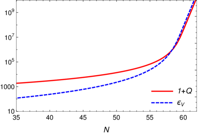
(a) Evolution case for $p=-1$, $c=0$ and $n=2$.

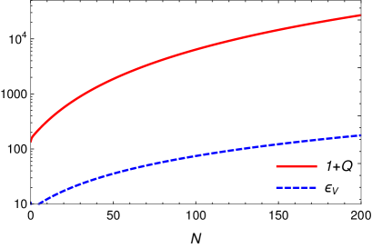
(b) Evolution case for $p=-1$, $c=0$ and $n=4$.

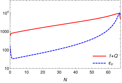
(c) Evolution case for $n=4$, but using Eq. (9).

Figure 1: Example cases for the evolution of $Q$ and $\epsilon_{V}$ with the number of $e$-foldings $N$. We have taken parameters analogous to those considered in Ref. Bastero-Gil:2019gao for convenience in this example.

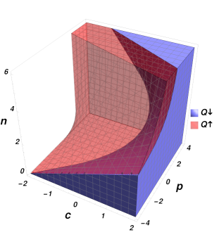
(a) 3d parameter space $(c,p,n)$

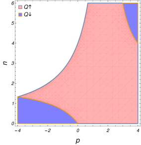
(b) Plane $c=0$

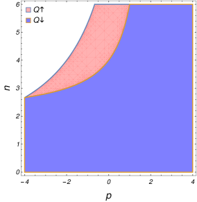
(c) Plane $c=2$

Figure 2: The parameter space for graceful exit in the case of the monomial class of inflaton potentials. The shaded areas indicate where $Q$ grows or decreases and WI has a graceful exit. Empty (white) space indicates where there is no graceful exit.

The above discussion shows that except for models with $p<2$, where WI is taking place in a strong dissipative regime, a form of potential yielding growing $\epsilon_{V}$ is sufficient to end inflation, just like in a cold inflation paradigm. Moreover, for the generic form of monomial potential Eq. (16), one gets a condition for graceful exit for models with $p<2$ (while WI is taking place in the strong dissipative regime) as

$$(2-p)n<8.$$ (24)

Therefore, considering for example the case for the WLI model Bastero-Gil:2016qru , with $p=1,c=0$, we obtain that $n<8$ in order to end inflation. This implies that the conventional monomial potentials, like the quartic and the quadratic, help end inflation in such a WI model. However, for the VWLI model Bastero-Gil:2019gao , when restricting to the case where the thermal mass $m(T)$ in Eq. (9) is dominated by the temperature dependent term, then the dissipative coefficient would effectively evolve as inverse of the temperature, yielding $p=-1,c=0$ as already explained before. In such a case, inflation only ends with a choice of a monomial potential with $n<8/3$ (while for $n<2/3$, $Q$ decreases, as can be seen from Eq. (18) and inflation ends without any further requirement). This is an important example case in WI, which demonstrates the importance of not only considering the phenomenological form of the dissipation coefficient but also the associated microscopic physics involved in the derivation of the model. To show this explicitly, in Fig. 1 we show the results for $\epsilon_{V}$ and $Q$ when evolving the background evolution equations, given by Eqs. (3), (4) and (5), and for three cases: For the dissipation coefficient Eq. (1) when taking $p=-1,c=0$ and in the case of a quadratic potential $n=2$ (panel a), for $p=-1,c=0$ and in the case of a quartic potential $n=4$ (panel b) and when using the explicit full form of the dissipation coefficient as derived from the microscopic physics, Eq. (9), also for the quartic potential (panel c). We see from the results shown in Fig. 1(a) that $\epsilon_{V}$ evolves faster than $Q$, thus ending inflation eventually. In Fig. 1(b), we show the evolution in the case of a quartic potential, $n=4$, where we see an opposite behavior, $\epsilon_{V}$ evolves slower than $Q$, thus never ending inflation. The behavior shown in Fig. 1 panels (a) and (b) is exactly what we have anticipated from the analysis done above. However, when considering the correct full form of the dissipation coefficient Eq. (9) in the case of the quartic potential, panel (c), inflation does end. This is because in the corresponding dynamics, as shown e.g. in Ref. Bastero-Gil:2019gao , the temperature decreases with the evolution. Thus, eventually the condition $m_{0}\ll\alpha T$ required to give a $\Upsilon\propto 1/T$ in Eq. (9) is no longer valid and the explicit form (9) will cause $Q$ to decrease faster as the system evolves, which eventually helps end inflation.

Let us now consider the more general case described in Eq. (19). For a monomial potential this condition reduces to

$$8-2p+[(p-2)n+8+4c]\,Q>0.$$ (25)

As we are dealing with the range $-4<p<4$, the above condition is easily satisfied when

$$(p-2)n>-8-4c.$$ (26)

We see from Eq. (18) that $Q$ increases when

$$(p-2)n>2p-4c.$$ (27)

For the range $-4<p<4$, the condition in Eq. (26) would also encompass Eq. (27). However, if $Q$ remains constant or decreases with $e$-foldings, in which case inflation ends even more easily, one would require $n\leq(2p-4c)/(p-2)$. In Fig. 2(a) we give the general prediction from the above inequalities, in the space of parameters $p,\,c$ and $n$, required for graceful exit in WI in the context of the class of monomial potentials Eq. (16). The regions for which $Q$ grows or decreases during WI and there is graceful exit have been identified. An empty (white) region indicates the parameter space where there is no graceful exit. The results shown in Figs. 2(b) and 2(c) exemplify the effect of having an inflaton field dependence in the dissipation coefficient. It tends to improve the available range of parameters allowing graceful exit in WI, but at the same time it decreases the area available (i.e., models) for which the dissipation ratio $Q$ grows and increases the one leading to a decreasing $Q$, which makes inflation ending more easily according to the general discussion given above.

One also notes from the above results that the type of graceful exit we discuss in the context of WI is mostly associated with the fact that $Q$ can grow faster than $\epsilon_{V}$ as already pointed out before. In this case, even if during inflation we might have the dynamics initially for $Q\ll 1$, i.e., start in the weak dissipative regime, it will certainly evolve towards the strong regime. As shown in Fig. 2, the regions for which WI does not end are essentially those for which $Q$ is growing. The CI dynamics would only be recovered in the opposite regime, when $Q$ decreases during the evolution and evolves to very small values at the end of inflation. In this case, the condition required for graceful exit would be similar to those in CI.

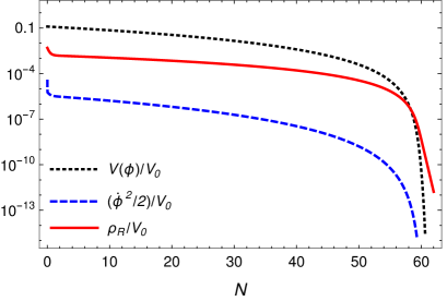
(a) Evolution case for $p=-1$, $c=0$ and $n=2$.

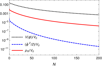
(b) Evolution case for $p=-1$, $c=0$ and $n=4$.

Figure 3: Example cases for the evolution of the energy densities with the number of $e$-foldings $N$. Parameters used were again based on the ones considered in Ref. Bastero-Gil:2019gao , corresponding e.g. to $C_{\Upsilon}\simeq 5.13$, $M\simeq 5.5\times 10^{-5}M_{\rm Pl}$ in Eq. (1), with an initial dissipation ratio $Q_{0}\simeq 100$.

As already emphasized in the Introduction, even though there is radiation production due to the dissipation, this does not mean that radiation will overtake the inflaton energy density and end inflation. This is illustrate by using again the example shown in Fig. 1 for the cases in panels (a) and (b). In Fig. 3 we show the evolution for the energy densities in the cases of an inversely proportional in the temperature dissipation coefficient for the cases of a quadratic (panel a) and quartic (panel b) inflaton potentials. These correspond to the cases where inflation can end in the former, which lies inside the red region shown in Fig. 2(b), and never end in the latter, which lies inside the white region shown in Fig. 2(b). Note that in the first case radiation overtakes the inflaton energy density ending inflation smoothly in a radiation dominated regime. In the second case there is always a nonvanishing radiation energy density being produced, yet it gets damped in a rate faster than the decrease in the inflaton energy density and inflation does not end. This behavior persists for much longer times (efoldings) than the ones shown in the figure.

III.1.2 Negative $\eta_{V}$

Next, we consider the case for concave inflaton potentials for which $\eta_{V}$ is negative. In such a case, the condition for graceful exit becomes

$$\epsilon_{V}\left[2(4-p)+(6+p)Q\right]+|\eta_{V}|\left(4-p+4Q\right)$$

$$+2c\,Q\,\kappa_{V}>0.$$ (28)

As an example, we can consider the hilltop-like class of potentials for the inflaton given by

$$V(\phi)=V_{0}\left[1-\left(\frac{\phi}{\phi_{0}}\right)^{2n}\right]^{2},$$ (29)

with $n\geq 1$ and with inflation taking place around the top (plateau) of the potential, $|\phi|\ll\phi_{0}$. We also consider that $\phi_{0}$ is sufficiently large such that inflation ends before the inflection point of the potential, thus, inflation takes place exactly in the concave part of the potential. The condition for graceful exit in this case then becomes $8n>2c+4$ in the regime of strong dissipation, while for weak dissipation we have that $8n>p(2n-1)+4$. In Fig. 4(a) we show the corresponding region for graceful exit, along also with the regions where we have a growing or decreasing $Q$. The Figs. 4(b) and 4(c) show the $c=0$ and $c=2$ planes, like what we have shown in the previous case. Notice that here all the parameter space allows for graceful exit.

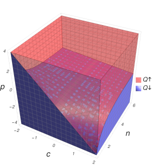
(a) 3d parameter space $(c,p,n)$

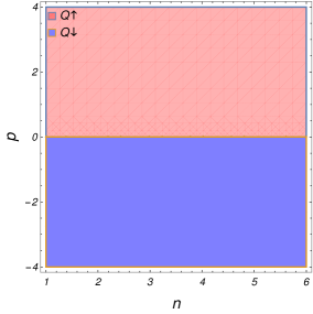
(b) Plane $c=0$

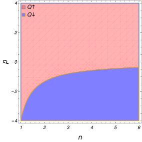
(c) Plane $c=2$

Figure 4: The parameter space for graceful exit in the case of the hilltop class of inflaton potentials Eq. (29). The shaded areas indicate where $Q$ grows or decreases and WI has a graceful exit.

Even though we have used in the above study the potential Eq. (29), it is easy to check that the results also apply to other classes of concave potentials. Thus, the concave potentials do lead generically to graceful exit in a WI setup. We also note that apart from WI taking place in strong dissipative regimes, a growing $\epsilon_{V}$ is sufficient to ensure graceful exit here, just as in cold inflation.

III.2 Constant $\epsilon_{V}$

Let us now consider the case of a constant $\epsilon_{V}$. Apart from the cosmological constant $\Lambda$, the classic example of such a potential is the runaway potential or the exponential potential,

$$V(\phi)=V_{0}e^{-\alpha\phi/M_{\rm Pl}},$$ (30)

which leads to constant slow-roll parameters $\eta_{V}=2\epsilon_{V}=\alpha^{2}$. Such a potential drives a power-law type inflation in cold inflation and does not lead to graceful exit Liddle:1988tb when $\alpha<\sqrt{2}$, while for $\alpha\geq\sqrt{2}$ there is not even an accelerated expansion.

However, if $Q$ decreases in a WI inflation setup, then there is a possibility to have both inflation and graceful exit in such inflationary scenarios when $\alpha>\sqrt{2}$. Accelerated expansion happens because we can arrange for $\epsilon_{V}=\alpha^{2}/2<1+Q$ for sufficiently large dissipation ratio $Q$. And graceful exit happens when $Q$ decreases. It is easy to see from Eq. (12) that $Q$ decreases when $p>2$ and it is independent of the value of $c$ whenever $\alpha\phi/M_{\rm Pl}>1$. This phenomenon has already been noted in Refs. Lima:2019yyv ; Goswami:2019ehb . It is to note that in this case, the inflaton will keep on slow-rolling if $Q$ keeps on increasing, and there will not be no graceful exit as such a runaway potential possesses no minimum (just as it happens in the case of cold inflation discussed above).

III.3 Decreasing $\epsilon_{V}$

Equation (15) tells us that $\epsilon_{V}$ decreases whenever

$$\frac{\epsilon_{V}}{\eta_{V}}<\frac{1}{2}.$$ (31)

Clearly, such potentials are not employed in cold inflation as they will not lead to graceful exit. However, as both $\epsilon_{V}$ and $Q$ can decrease simultaneously in WI, there is a sliver of chance that inflation might end in such scenarios. One such potential of the form

$$V(\phi)=V_{0}\left(1+e^{-\alpha\phi/M_{\rm Pl}}\right),$$ (32)

has been employed in the MWI model recently Goswami:2019ehb . However, it is to note that WI takes place when $\epsilon_{V}<1+Q$. Then, in such decreasing $\epsilon_{V}$ scenario, one needs to start with $\epsilon_{V}>1$ and $Q$ not only requires to fall faster than $\epsilon_{V}$ but it must fall much faster such that $1+Q$ crosses $\epsilon_{V}$ before $\epsilon_{V}$ decreases below unity. Fulfilling such a condition is rather challenging and inflation would not end in such scenarios in most of the cases.

We have evolved the full background equations with the above potential applied in the MWI model (e.g., $p=3,c=0$), and have showed in Fig. 5 the typical behavior of $\epsilon_{V}$ and $Q$ in such scenarios. As shown in the example of Fig. 5, even though $Q$ starts to decrease faster than $\epsilon_{V}$ initially, it does not fall faster enough. $\epsilon_{V}$ eventually drops below unity and $1+Q$ saturates to 1, and, hence, inflation is not terminated.

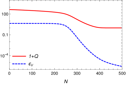
Figure 5: Typical behavior of $Q$ and $\epsilon_{V}$ in the MWI model and with a form a potential given in Eq. (32).

IV Further discussions and possible applications

Let us discuss some possible applications of the results obtained in this paper.

We should recall that the primordial spectrum of scalar curvature perturbations is strongly affected by the dissipation in WI Graham:2009bf ; BasteroGil:2011xd ; Ramos:2013nsa ; Bastero-Gil:2014jsa ; Li:2018wno . In particular, a dynamical regime for which $Q$ grows invariably leads to a growing spectral tilt $n_{s}$, thus to a bluer spectrum. In the opposite regime, for which we have a decreasing $Q$, the effect has been shown to produce a decreasing $n_{s}$, i.e., a redder spectrum (for systematic analysis of the effect of the behavior of the dissipation on the power spectrum, see, e.g., Refs. Graham:2009bf ; BasteroGil:2011xd ; Bastero-Gil:2014jsa ). To see these effects explicitly on the observables, let us recall that in WI the primordial curvature power spectrum is of the general form Ramos:2013nsa ; Benetti:2016jhf

$$\Delta_{{\cal R}}(k)=\left(\frac{H^{2}}{2\pi\dot{\phi}}\right)^{2}{\cal F}(Q),$$ (33)

where all quantities are meant to be evaluated at the Hubble radius crossing, $k=aH$. The function ${\cal F}(Q)$ in Eq. (33) strongly depends on the form of the dissipation coefficient and the consequent dynamics (see, e.g., Refs. Graham:2009bf ; BasteroGil:2011xd ; Bastero-Gil:2014jsa ). From Eq. (33), the spectral tilt $n_{s}$ is defined as

$$n_{s}-1 = \frac{d\ln\Delta_{{\cal R}}(k)}{d\ln k}\simeq\frac{d\ln\Delta_{{\cal R}}(k)}{dN}$$ (34)

$$\simeq \frac{-6\epsilon_{V}+2\eta_{V}+2\frac{dQ}{dN}}{1+Q}+\frac{dQ}{dN}\frac{d\ln{\cal F}(Q)}{dQ}.$$

Typically, the last term dominates in many of the WI realizations. Thus, for WI models for which $Q$ grows with the number of efolds but have a decreasing ${\cal F}(Q)$ with $Q$, like e.g., in the models with a dissipation coefficient with negative powers in the temperature Motaharfar:2018zyb , they will lead to a redder scalar power spectrum. Other models leading also to a growing $Q$ with the number of efolds but an increasing ${\cal F}(Q)$ with $Q$ will lead to a bluer spectrum. Similarly, a decreasing $Q$ with $N$ will have an effect on the observables. Hence, we see that the dynamical behavior of the dissipation ratio is fundamental to determine whether we can have a redder or bluer spectrum. Thus, determining possible regimes for a growing or decreasing dissipation ratio can be of fundamental relevance for WI model building. For instance, models that in the cold inflation context are excluded because the spectrum is too red or it is too blue, can be rendered observationally consistent in the WI picture by choosing models leading to either a growing or to a decreasing dissipation ratio, respectively.

It is important to also point out that the issue of graceful exit in WI may not be a negative feature but in some cases might be a desirable outcome. A sustained acceleration regime in the late Universe, attributed to dark energy, might conceivably emerge as a special case of an overdamped dynamical regime for a scalar field. In this case, given a potential with a minimum at $\phi=\phi_{0}$ and if the approach to $\phi_{0}$ is asymptotic, as discussed above in the context of the graceful exit problem in WI, the scalar field can remain close to the minimum $\phi_{0}$, then with $V(\phi\neq\phi_{0})>0$ the evolution would mimic closely that of a cosmological constant. This is particularly important when the energy density varies very slowly. For instance, from the slow-roll equations (10), we can deduce that the rate of change of the energy density of the scalar field in a Hubble time can be expressed as Bartrum:2014fla

$$\frac{1}{H}\left|\frac{\dot{\rho}_{\phi}}{\rho_{\phi}}\right|\simeq 2\frac{\rho_{\phi}}{\rho_{\rm total}}\epsilon_{wi}\ll 1,$$ (35)

where we have also used Eq. (7) and $\rho_{\rm total}$ denotes the total energy density at that given time in the late-time Universe, where we also expect that $\rho_{\phi}\ll\rho_{\rm total}$, if the energy density of the scalar field is not the dominant energy component. The result given by Eq. (35) shows that whenever $\epsilon_{wi}\ll 1$, which happens in particular when the conditions for not having graceful exit and that we have discussed are met, then the scalar field dissipates very little of its energy density on cosmological time scales. Thus, the overdamped regime that can potentially lead to a graceful exit problem in the early Universe, at late times can also potentially sustain a (slowly-varying) cosmological vacuum energy term mimicking a cosmological constant. Thus, the result we have obtained in the present paper can certainly be used as a guide in the development of possible quintessential-like scalar field models where the late-time accelerated expansion might eventually emerge as a consequence of dissipative effects (see, e.g., Ref. Lima:2019yyv for a specific attempt in this context).

V Conclusions

To conclude, we have shown that the process of graceful exit in WI is a more rich phenomenon than it is in cold inflation. Graceful exit in WI depends on three independent choices: The form of the potential (hence the behavior of $\epsilon_{V}$ during inflation), the choice of the WI model (hence the form of the dissipative coefficient) and whether we want WI to take place in a weak or in a strong dissipative regime. However, we have shown that there are cases, where a potential with growing $\epsilon_{V}$ in time (or with $e$-foldings) is good enough to exit WI gracefully, as it happens in a cold paradigm. This happens in the cases of inflation happening in the plateau region of the concave potentials or in cases where $Q$ is decreasing with $e$-foldings. In the rest of the cases, one needs to make sure that $\epsilon_{V}$ grows faster than $Q$ in order to exit gracefully. We have also shown that WI is capable of terminating inflation even in cases where cold inflation fails to exit gracefully, such as in the case of runaway potentials.

It is to note that the reason behind no graceful exit in these cases of WI differs from the usual reason of getting trapped in a false vacuum, as it happens in cold inflation. Mostly, $Q$ increasing faster than $\epsilon_{V}$ (where $\epsilon_{V}$ evolves) or a simply growing $Q$ in cases of constant $\epsilon_{V}$ leads to no graceful exit in WI. It is to recall that the parameter $Q$ incorporates extra frictional term in the equation of motion of the inflaton field, and an increasing $Q$, in these cases, will make such an equation overdamped. Therefore inflation can only end in an asymptotic time, resulting in a realizing of never-ending inflation, and hence no graceful exit.

The situation is particularly delicate in the case of chaotic like monomial potentials. In this case, not all parameter space allows graceful exit, as far as the simple parametrization for the dissipation coefficient, given by Eq. (1), is concerned. We have demonstrated the issues involved in this case in an example making use of a dissipation coefficient $\Upsilon\propto 1/T$. In this case, the simple parametrization Eq. (1) is not enough to get the complete dynamics in WI and for studying graceful exit. We have also to consider the microscopic physics leading to this coefficient and the consistency conditions leading to the simple form for the dissipation coefficient. Given that most phenomenological studies involving WI make use of the simple parametrization given by Eq. (1), these results prompt to a word of caution in the studies of the dynamics in those models if details of the possible microscopic physics are left unchecked. Likewise, we have also shown that whether or not the dissipation coefficient depends on the inflaton amplitude can change the conclusions regarding graceful exit in a significant way.

Our study that we have performed in this paper have also identified regimes for which the dissipation ratio $Q$ can either grow or decrease with the number of efolds, depending on the different combinations of dissipation coefficient and primordial potentials. This is particularly important in the context of obtaining observational predictions in WI. It would also be interesting to carry out a similar analysis as the one performed here to other dynamics involving WI, like in noncanonical type of models Li:2018riw ; Zhang:2019bgv ; Zhang:2020sbk .

References

- (1) A. Berera, “Warm inflation,” Phys. Rev. Lett. 75, 3218-3221 (1995) doi:10.1103/PhysRevLett.75.3218 [arXiv:astro-ph/9509049 [astro-ph]].
- (2) M. Bastero-Gil, A. Berera, R. O. Ramos and J. G. Rosa, “Towards a reliable effective field theory of inflation,” Phys. Lett. B 813, 136055 (2021) doi:10.1016/j.physletb.2020.136055 [arXiv:1907.13410 [hep-ph]].
- (3) V. Kamali, M. Motaharfar and R. O. Ramos, “Warm brane inflation with an exponential potential: a consistent realization away from the swampland,” Phys. Rev. D 101, no.2, 023535 (2020) doi:10.1103/PhysRevD.101.023535 [arXiv:1910.06796 [gr-qc]].
- (4) S. Das and R. O. Ramos, “Runaway potentials in warm inflation satisfying the swampland conjectures,” Phys. Rev. D 102, no.10, 103522 (2020) doi:10.1103/PhysRevD.102.103522 [arXiv:2007.15268 [hep-th]].
- (5) Y. Akrami et al. [Planck], “Planck 2018 results. X. Constraints on inflation,” Astron. Astrophys. 641, A10 (2020) doi:10.1051/0004-6361/201833887 [arXiv:1807.06211 [astro-ph.CO]].
- (6) J. C. Bueno Sanchez, M. Bastero-Gil, A. Berera, K. Dimopoulos and K. Kohri, “The gravitino problem in supersymmetric warm inflation,” JCAP 03, 020 (2011) doi:10.1088/1475-7516/2011/03/020 [arXiv:1011.2398 [hep-ph]].
- (7) S. Bartrum, A. Berera and J. G. Rosa, “Gravitino cosmology in supersymmetric warm inflation,” Phys. Rev. D 86, 123525 (2012) doi:10.1103/PhysRevD.86.123525 [arXiv:1208.4276 [hep-ph]].
- (8) M. Bastero-Gil, A. Berera, R. O. Ramos and J. G. Rosa, “Warm baryogenesis,” Phys. Lett. B 712, 425-429 (2012) doi:10.1016/j.physletb.2012.05.032 [arXiv:1110.3971 [hep-ph]].
- (9) M. Bastero-Gil, A. Berera, R. O. Ramos and J. G. Rosa, “Observational implications of mattergenesis during inflation,” JCAP 10, 053 (2014) doi:10.1088/1475-7516/2014/10/053 [arXiv:1404.4976 [astro-ph.CO]].
- (10) M. Benetti and R. O. Ramos, “Warm inflation dissipative effects: predictions and constraints from the Planck data,” Phys. Rev. D 95, no.2, 023517 (2017) doi:10.1103/PhysRevD.95.023517 [arXiv:1610.08758 [astro-ph.CO]].
- (11) A. Berera, J. Mabillard, M. Pieroni and R. O. Ramos, “Identifying Universality in Warm Inflation,” JCAP 07, 021 (2018) doi:10.1088/1475-7516/2018/07/021 [arXiv:1803.04982 [astro-ph.CO]].
- (12) M. Bastero-Gil, A. Berera, R. Brandenberger, I. G. Moss, R. O. Ramos and J. G. Rosa, “The role of fluctuation-dissipation dynamics in setting initial conditions for inflation,” JCAP 01, 002 (2018) doi:10.1088/1475-7516/2018/01/002 [arXiv:1612.04726 [astro-ph.CO]].
- (13) A. Berera, M. Gleiser and R. O. Ramos, “Strong dissipative behavior in quantum field theory,” Phys. Rev. D 58, 123508 (1998) doi:10.1103/PhysRevD.58.123508 [arXiv:hep-ph/9803394 [hep-ph]].
- (14) J. Yokoyama and A. D. Linde, “Is warm inflation possible?,” Phys. Rev. D 60, 083509 (1999) doi:10.1103/PhysRevD.60.083509 [arXiv:hep-ph/9809409 [hep-ph]].
- (15) A. Berera, I. G. Moss and R. O. Ramos, “Warm Inflation and its Microphysical Basis,” Rept. Prog. Phys. 72, 026901 (2009) doi:10.1088/0034-4885/72/2/026901 [arXiv:0808.1855 [hep-ph]].
- (16) M. Bastero-Gil, A. Berera, R. O. Ramos and J. G. Rosa, “General dissipation coefficient in low-temperature warm inflation,” JCAP 01, 016 (2013) doi:10.1088/1475-7516/2013/01/016 [arXiv:1207.0445 [hep-ph]].
- (17) S. Bartrum, M. Bastero-Gil, A. Berera, R. Cerezo, R. O. Ramos and J. G. Rosa, “The importance of being warm (during inflation),” Phys. Lett. B 732, 116-121 (2014) doi:10.1016/j.physletb.2014.03.029 [arXiv:1307.5868 [hep-ph]].
- (18) M. Bastero-Gil, A. Berera, R. O. Ramos and J. G. Rosa, “Warm Little Inflaton,” Phys. Rev. Lett. 117, no.15, 151301 (2016) doi:10.1103/PhysRevLett.117.151301 [arXiv:1604.08838 [hep-ph]].
- (19) K. V. Berghaus, P. W. Graham and D. E. Kaplan, “Minimal Warm Inflation,” JCAP 03, 034 (2020) doi:10.1088/1475-7516/2020/03/034 [arXiv:1910.07525 [hep-ph]].
- (20) M. Bastero-Gil, A. Berera and R. O. Ramos, “Dissipation coefficients from scalar and fermion quantum field interactions,” JCAP 09, 033 (2011) doi:10.1088/1475-7516/2011/09/033 [arXiv:1008.1929 [hep-ph]].
- (21) G. Obied, H. Ooguri, L. Spodyneiko and C. Vafa, “De Sitter Space and the Swampland,” [arXiv:1806.08362 [hep-th]].
- (22) S. K. Garg and C. Krishnan, “Bounds on Slow Roll and the de Sitter Swampland,” JHEP 11, 075 (2019) doi:10.1007/JHEP11(2019)075 [arXiv:1807.05193 [hep-th]].
- (23) H. Ooguri, E. Palti, G. Shiu and C. Vafa, “Distance and de Sitter Conjectures on the Swampland,” Phys. Lett. B 788, 180-184 (2019) doi:10.1016/j.physletb.2018.11.018 [arXiv:1810.05506 [hep-th]].
- (24) W. H. Kinney, S. Vagnozzi and L. Visinelli, “The zoo plot meets the swampland: mutual (in)consistency of single-field inflation, string conjectures, and cosmological data,” Class. Quant. Grav. 36, no.11, 117001 (2019) doi:10.1088/1361-6382/ab1d87 [arXiv:1808.06424 [astro-ph.CO]].
- (25) S. Das, “Note on single-field inflation and the swampland criteria,” Phys. Rev. D 99, no.8, 083510 (2019) doi:10.1103/PhysRevD.99.083510 [arXiv:1809.03962 [hep-th]].
- (26) M. Motaharfar, V. Kamali and R. O. Ramos, “Warm inflation as a way out of the swampland,” Phys. Rev. D 99, no.6, 063513 (2019) doi:10.1103/PhysRevD.99.063513 [arXiv:1810.02816 [astro-ph.CO]].
- (27) S. Das, “Warm Inflation in the light of Swampland Criteria,” Phys. Rev. D 99, no.6, 063514 (2019) doi:10.1103/PhysRevD.99.063514 [arXiv:1810.05038 [hep-th]].
- (28) M. Bastero-Gil, A. Berera, R. Hernández-Jiménez and J. G. Rosa, “Warm inflation within a supersymmetric distributed mass model,” Phys. Rev. D 99, no.10, 103520 (2019) doi:10.1103/PhysRevD.99.103520 [arXiv:1812.07296 [hep-ph]].
- (29) S. Das, “Distance, de Sitter and Trans-Planckian Censorship conjectures: the status quo of Warm Inflation,” Phys. Dark Univ. 27, 100432 (2020) doi:10.1016/j.dark.2019.100432 [arXiv:1910.02147 [hep-th]].
- (30) A. Berera and J. R. Calderón, “Trans-Planckian censorship and other swampland bothers addressed in warm inflation,” Phys. Rev. D 100, no.12, 123530 (2019) doi:10.1103/PhysRevD.100.123530 [arXiv:1910.10516 [hep-ph]].
- (31) S. Das, G. Goswami and C. Krishnan, “Swampland, axions, and minimal warm inflation,” Phys. Rev. D 101, no.10, 103529 (2020) doi:10.1103/PhysRevD.101.103529 [arXiv:1911.00323 [hep-th]].
- (32) R. Brandenberger, V. Kamali and R. O. Ramos, “Strengthening the de Sitter swampland conjecture in warm inflation,” JHEP 08, 127 (2020) doi:10.1007/JHEP08(2020)127 [arXiv:2002.04925 [hep-th]].
- (33) A. Berera, S. Brahma and J. R. Calderón, “Role of trans-Planckian modes in cosmology,” JHEP 08, 071 (2020) doi:10.1007/JHEP08(2020)071 [arXiv:2003.07184 [hep-th]].
- (34) M. Bastero-Gil and A. Berera, “Warm inflation model building,” Int. J. Mod. Phys. A 24, 2207-2240 (2009) doi:10.1142/S0217751X09044206 [arXiv:0902.0521 [hep-ph]].
- (35) Y. Zhang, “Warm Inflation With A General Form Of The Dissipative Coefficient,” JCAP 03, 023 (2009) doi:10.1088/1475-7516/2009/03/023 [arXiv:0903.0685 [hep-ph]].
- (36) M. Gleiser and R. O. Ramos, “Microphysical approach to nonequilibrium dynamics of quantum fields,” Phys. Rev. D 50, 2441-2455 (1994) doi:10.1103/PhysRevD.50.2441 [arXiv:hep-ph/9311278 [hep-ph]].
- (37) R. Herrera, M. Olivares and N. Videla, “General dissipative coefficient in warm intermediate and logamediate inflation,” Phys. Rev. D 88, 063535 (2013) doi:10.1103/PhysRevD.88.063535 [arXiv:1310.0780 [gr-qc]].
- (38) R. Herrera, M. Olivares and N. Videla, “General dissipative coefficient in warm intermediate inflation in loop quantum cosmology in light of Planck and BICEP2,” Int. J. Mod. Phys. D 23, no.10, 1450080 (2014) doi:10.1142/S0218271814500801 [arXiv:1404.2803 [gr-qc]].
- (39) L. Visinelli, “Observational Constraints on Monomial Warm Inflation,” JCAP 07, 054 (2016) doi:10.1088/1475-7516/2016/07/054 [arXiv:1605.06449 [astro-ph.CO]].
- (40) A. Jawad, N. Videla and F. Gulshan, “Dynamics of warm power-law plateau inflation with a generalized inflaton decay rate: predictions and constraints after Planck 2015,” Eur. Phys. J. C 77, no.5, 271 (2017) doi:10.1140/epjc/s10052-017-4846-1 [arXiv:1704.07005 [gr-qc]].
- (41) A. Jawad, S. Hussain, S. Rani and N. Videla, “Impact of generalized dissipative coefficient on warm inflationary dynamics in the light of latest Planck data,” Eur. Phys. J. C 77, no.10, 700 (2017) doi:10.1140/epjc/s10052-017-5264-0 [arXiv:1709.10430 [gr-qc]].
- (42) I. G. Moss and C. Xiong, “On the consistency of warm inflation,” JCAP 11, 023 (2008) doi:10.1088/1475-7516/2008/11/023 [arXiv:0808.0261 [astro-ph]].
- (43) S. del Campo, R. Herrera, D. Pavón and J. R. Villanueva, “On the consistency of warm inflation in the presence of viscosity,” JCAP 08, 002 (2010) doi:10.1088/1475-7516/2010/08/002 [arXiv:1007.0103 [astro-ph.CO]].
- (44) M. Bastero-Gil, A. Berera, R. Cerezo, R. O. Ramos and G. S. Vicente, “Stability analysis for the background equations for inflation with dissipation and in a viscous radiation bath,” JCAP 11, 042 (2012) doi:10.1088/1475-7516/2012/11/042 [arXiv:1209.0712 [astro-ph.CO]].
- (45) A. R. Liddle, “Power Law Inflation With Exponential Potentials,” Phys. Lett. B 220, 502-508 (1989) doi:10.1016/0370-2693(89)90776-4
- (46) G. B. F. Lima and R. O. Ramos, “Unified early and late Universe cosmology through dissipative effects in steep quintessential inflation potential models,” Phys. Rev. D 100, no.12, 123529 (2019) doi:10.1103/PhysRevD.100.123529 [arXiv:1910.05185 [astro-ph.CO]].
- (47) C. Graham and I. G. Moss, “Density fluctuations from warm inflation,” JCAP 07, 013 (2009) doi:10.1088/1475-7516/2009/07/013 [arXiv:0905.3500 [astro-ph.CO]].
- (48) M. Bastero-Gil, A. Berera and R. O. Ramos, “Shear viscous effects on the primordial power spectrum from warm inflation,” JCAP 07, 030 (2011) doi:10.1088/1475-7516/2011/07/030 [arXiv:1106.0701 [astro-ph.CO]].
- (49) R. O. Ramos and L. A. da Silva, “Power spectrum for inflation models with quantum and thermal noises,” JCAP 03, 032 (2013) doi:10.1088/1475-7516/2013/03/032 [arXiv:1302.3544 [astro-ph.CO]].
- (50) M. Bastero-Gil, A. Berera, I. G. Moss and R. O. Ramos, “Cosmological fluctuations of a random field and radiation fluid,” JCAP 05, 004 (2014) doi:10.1088/1475-7516/2014/05/004 [arXiv:1401.1149 [astro-ph.CO]].
- (51) X. B. Li, H. Wang and J. Y. Zhu, “Gravitational waves from warm inflation,” Phys. Rev. D 97, no.6, 063516 (2018) doi:10.1103/PhysRevD.97.063516 [arXiv:1803.10074 [gr-qc]].
- (52) S. Bartrum, A. Berera and J. G. Rosa, “Fluctuation-dissipation dynamics of cosmological scalar fields,” Phys. Rev. D 91, no.8, 083540 (2015) doi:10.1103/PhysRevD.91.083540 [arXiv:1412.5489 [hep-ph]].
- (53) K. Li, X. M. Zhang, H. Y. Ma and J. Y. Zhu, “Noncanonical warm inflation: a model with a general Lagrangian density,” Phys. Rev. D 98, no.12, 123528 (2018) doi:10.1103/PhysRevD.98.123528 [arXiv:1804.00276 [gr-qc]].
- (54) X. M. Zhang, K. Li, H. Y. Ma, Q. Liu and J. Y. Zhu, “Non-Gaussianity in a general kind noncanonical warm inflation,” Phys. Rev. D 100, no.12, 123521 (2019) doi:10.1103/PhysRevD.100.123521 [arXiv:1910.01390 [gr-qc]].
- (55) X. M. Zhang, A. Fu, K. Li, Q. Liu, P. C. Chu, H. Y. Ma and J. Y. Zhu, “Consistency of a kind of general noncanonical warm inflation,” Phys. Rev. D 103, no.2, 023511 (2021) doi:10.1103/PhysRevD.103.023511 [arXiv:2011.14623 [gr-qc]].