Adaptive Learning of the Optimal Batch Size of SGD

Abstract

Recent advances in the theoretical understanding of SGD [Qian et al. (2019)] led to a formula for the optimal batch size minimizing the number of effective data passes, i.e., the number of iterations times the batch size. However, this formula is of no practical value as it depends on the knowledge of the variance of the stochastic gradients evaluated at the optimum. In this paper we design a practical SGD method capable of learning the optimal batch size adaptively throughout its iterations for strongly convex and smooth functions. Our method does this provably, and in our experiments with synthetic and real data robustly exhibits nearly optimal behaviour; that is, it works as if the optimal batch size was known a-priori. Further, we generalize our method to several new batch strategies not considered in the literature before, including a sampling suitable for distributed implementations.

1 Introduction

Stochastic Gradient Descent (SGD), in one disguise or another, is undoubtedly the backbone of modern systems for training supervised machine learning models [Robbins and Monro (1951), Nemirovski et al. (2009), Bottou (2010)]. The method earns its popularity due to its superior performance on very large datasets where more traditional methods such as gradient descent (GD), relying on a pass through the entire training dataset before adjusting the model parameters, are simply too slow to be useful. In contrast, SGD in each iteration uses a small portion of the training data only (a batch) to adjust the model parameters, and this process repeats until a model of suitable quality is found. In practice, batch SGD is virtually always applied to a finite-sum problem of the form $\textstyle x^{*}=\arg\min\limits_{x\in\mathbb{R}^{d}}\frac{1}{n}\sum\limits_{i=1}^{n}f_{i}(x),$ where $n$ is the number of training data and $f(x)=\frac{1}{n}\sum_{i=1}^{n}f_{i}(x)$ represents the average loss, i.e. empirical risk, of model $x$ on the training dataset. With this formalism in place, a generic batch SGD method performs the iteration $\textstyle x^{k+1}=x^{k}-\gamma^{k}\sum\limits_{i\in S^{k}}v_{i}^{k}\nabla f_{i}(x^{k}),$ where $S^{k}\subseteq\{1,2,\dots,n\}$ is the batch considered in iteration $k$ and $v_{1}^{k},\dots,v_{n}^{k}$ are appropriately chosen scalars. Often in practice, and almost invariably in theory, the batch $S^{k}$ is chosen at random according to some fixed probability law, and the scalars $v_{i}^{k}$ are chosen to ensure that $g^{k}=\sum\limits_{i\in S^{k}}v_{i}^{k}\nabla f_{i}(x^{k})$ is an unbiased estimator of the gradient $\nabla f(x^{k})$. One standard choice is to fix a batch size $\tau\in\{1,2,\dots,n\}$, and pick $S^{k}$ uniformly from all subsets of size $\tau$. Another option is to partition the training dataset into $n/\tau$ subsets of size $\tau$, and then in each iteration let $S^{k}$ to be one of these partitions, chosen with some probability, e.g., uniformly.

Contributions Effective online learning of the optimal batch size. We make a step towards the development of a practical variant of optimal batch SGD, aiming to learn the optimal batch size $\tau^{*}$ on the fly. To the best of our knowledge, our method (Algorithm 3) is the first variant of SGD able to learn the optimal batch. Sampling strategies. We do not limit our selves to the uniform sampling strategy we used for illustration purposes above and develop closed-form expressions for the optimal batch size for several other sampling techniques. Our adaptive method works well for all of them. Convergence theory. We prove that our adaptive method converges, and moreover learns the optimal batch size. Practical robustness. We show the algorithm’s robustness by conducting extensive experiments using different sampling techniques and different machine learning models on both real and synthetic datasets.

Related work A stream of research attempts to boost the performance of SGD in practice is tuning its hyperparameters such as learning rate, and batch size while training. In this context, a lot of work has been done in proposing various learning rate schedulers [Schumer and Steiglitz (1968), Mathews and Xie (1993), Barzilai and Borwein (1988), Zeiler (2012), Tan et al. (2016), Shin et al. (2017)]. De et al. (2017) showed that one can reduce the variance by increasing the batch size without decreasing step-size (to maintain the constant signal to noise ratio). Besides, Smith et al. (2019) demonstrated the effect of increasing the batch size instead of decreasing the learning rate in training a deep neural network. However, most of these strategies are based on empirical results only. You et al. (2017a, b) show empirically the advantage of training on large batch size, while Masters and Luschi (2018) claim that it is preferable to train on smaller one.

SGD Overview. To study batch SGD for virtually all (stationary) subsampling rules, we adopt the stochastic reformulation paradigm for finite-sum problems proposed in Qian et al. (2019). The random vector $v\in\mathbb{R}^{n}$ is sampled from a distribution $\mathcal{D}$ and satisfies $\mathbb{E}_{\mathcal{D}}[v_{i}]=1$. Typically, the vector $v$ is defined by first choosing a random batch $\mathcal{S}^{k}\subseteq\{1,2,\dots,n\}$, then defining $v_{i}^{k}=0$ for $i\notin\mathcal{S}^{k}$, and choosing $v_{i}^{k}$ to an appropriate value for $i\notin\mathcal{S}^{k}$ in order to make sure the stochastic gradient $\nabla f_{v^{k}}(x^{k})$ is unbiased. In this work, we consider two particular choices of the probability law governing the selection of $\mathcal{S}^{k}$.

$\tau-$partition nice sampling In this sampling, we divide the training set into partitions $\mathcal{C}_{j}$ (of possibly different sizes $n_{\mathcal{C}_{j}}$), and each of them has at least a cardinality of $\tau$. At each iteration, one of the sets $\mathcal{C}_{j}$ is chosen with probability $q_{\mathcal{C}_{j}}$, and then $\tau-$nice sampling (without replacement) is applied on the chosen set. For each subset $C$ cardinality $\tau$ of partition $C_{j}$ cardinality $n_{C_{j}}$, $\mathbb{P}[v_{C}=\mathbbm{1}_{C\in\mathcal{S}}]=q_{j}/\binom{n_{C_{j}}}{\tau}$. $\tau-$partition independent sampling Similar to $\tau-$partition nice sampling, we divide the training set into partitions $\mathcal{C}_{j}$, and each of them has at least a cardinality of $\tau$. At each iteration one of the sets $\mathcal{C}_{j}$ is chosen with probability $q_{\mathcal{C}_{j}}$, and then $\tau-$independent sampling is applied on the chosen set. For each element $i$ of partition $C_{j}$, we have $\mathbb{P}[v_{i}=\mathbbm{1}_{C\in\mathcal{S}}]=q_{j}p_{i}$. The stochastic formulation naturally leads to the following concept of expected smoothness.

Assumption 1

The function $f$ is $\mathcal{L}-$smooth with respect to a datasets $\mathcal{D}$ if there exist $\mathcal{L}>0$ with

$$\mathbb{E}_{\mathcal{D}}\left[\left\|\nabla f_{v}(x)-\nabla f_{v}(x^{*})\right\|^{2}\right]\leq 2\mathcal{L}(f(x)-f(x^{*})).$$ (1)

Assumption 2

The gradient noise ${\sigma}={\sigma}(x^{*})$, where ${\sigma}(x):=\mathbb{E}_{\mathcal{D}}[\left\|\nabla f_{v}(x)\right\|^{2}],$ is finite.

Theorem 1.1.

Assume $f$ is $\mu-$strongly convex and Assumptions 1, 2 are satisfied. For any $\epsilon>0$, if the learning rate $\gamma$ is set to be

$$\gamma=\tfrac{1}{2}\min\left\{\tfrac{1}{\mathcal{L}},\tfrac{\epsilon\mu}{2{\sigma}}\right\}\quad\text{and}\quad k\geq\tfrac{2}{\mu}\max\left\{\mathcal{L},\tfrac{2{\sigma}}{\epsilon\mu}\right\}\log\left(\tfrac{2\|x^{0}-x^{*}\|^{2}}{\epsilon}\right)\,\,\text{then}\,\,\mathbb{E}\left\|x^{k}-x^{*}\right\|^{2}\leq\epsilon$$ (2)

2 Deriving Optimal Batch Size

After giving this thorough introduction to the stochastic reformulation of SGD, we can move on to study the effect of the batch size on the total iteration complexity. In fact, for each sampling technique, the batch size will affect both the expected smoothness $\mathcal{L}$ and the gradient noise ${\sigma}$. This effect reflects on the number of iterations required to reach to $\epsilon$ neighborhood around the optimum.

Formulas for $\mathcal{L}$ and $\sigma$ Before proceeding, we establish some terminologies. In addition of having $f$ to be $L-$smooth, we also assume each $f_{i}$ to be $L_{i}-$smooth. In $\tau-$partition samplings (both nice and independent), let $n_{\mathcal{C}_{j}}$ be number of data-points in the partition $\mathcal{C}_{j}$, where $n_{\mathcal{C}_{j}}\geq\tau$. Let $L_{\mathcal{C}_{j}}$ be the smoothness constants of the function $f_{\mathcal{C}_{j}}=\tfrac{1}{n_{\mathcal{C}_{j}}}\sum_{i\in\mathcal{C}_{j}}f_{i}$. Also, let $\overline{L}_{\mathcal{C}_{j}}=\tfrac{1}{n_{\mathcal{C}_{j}}}\sum_{i\in\mathcal{C}_{j}}L_{i}$ be the average of the Lipschitz smoothness constants of the functions in partition $\mathcal{C}_{j}$. In addition, let $h_{\mathcal{C}_{j}}(x)=\left\|\nabla f_{\mathcal{C}_{j}}(x)\right\|^{2}$ be the norm of the gradient of $f_{\mathcal{C}_{j}}$ at $x$. Finally, let $\overline{h}_{\mathcal{C}_{j}}(x)=\tfrac{1}{n_{\mathcal{C}_{j}}}\sum_{i\in C_{j}}h_{i}(x)$. For ease of notation, we will drop $x$ from all of the expression since it is understood from the context $(h_{i}=h_{i}(x))$. Also, superscripts with $(*,k)$ refer to evaluating the function at $x^{*}$ and $x^{k}$ respectively $(e.g.\,\,h_{i}^{*}=h_{i}(x^{*}))$. Now we introduce our key lemma, which gives an estimate of the expected smoothness for different sampling techniques.

Lemma 2.1.

For the considered samplings, the expected smoothness constants $\mathcal{L}$ can be upper bounded by $\mathcal{L}(\tau)$ (i.e. $\mathcal{L}\leq\mathcal{L}(\tau)$), where $\mathcal{L}(\tau)$ is expressed as follows

(i) For $\tau$-partition nice sampling,$\mathcal{L}(\tau)=\tfrac{1}{n\tau}\max_{\mathcal{C}_{j}}\tfrac{n_{\mathcal{C}_{j}}}{q_{\mathcal{C}_{j}}(n_{\mathcal{C}_{j}}-1)}\Big{[}(\tau-1)L_{\mathcal{C}_{j}}n_{\mathcal{C}_{j}}+(n_{\mathcal{C}_{j}}-\tau)\max_{i\in{\mathcal{C}_{j}}}{L_{i}}\Big{]}.$

(ii) For $\tau$-partition independent sampling, we have: $\mathcal{L}(\tau)=\tfrac{1}{n}\max_{\mathcal{C}_{j}}{\tfrac{n_{\mathcal{C}_{j}}L_{\mathcal{C}_{j}}}{q_{\mathcal{C}_{j}}}+\max_{i\in C_{j}}{\tfrac{L_{i}(1-p_{i})}{q_{C_{j}}p_{i}}}}.$

For the considered samplings, the gradient noise is given by ${\sigma}(x^{*},\tau)$, where

(i) For $\tau$-partition nice sampling,${\sigma}(x,\tau)=\tfrac{1}{n^{2}\tau}\sum_{\mathcal{C}_{j}}\tfrac{n_{\mathcal{C}_{j}}^{2}}{q_{\mathcal{C}_{j}}(n_{\mathcal{C}_{j}}-1)}\Big{[}(\tau-1)h_{\mathcal{C}_{j}}n_{\mathcal{C}_{j}}+(n_{\mathcal{C}_{j}}-\tau)\overline{h}_{\mathcal{C}_{j}}\Big{]}.$

(ii) For $\tau-$partition independent sampling, we have $\mathcal{{\sigma}}(x,\tau)=\tfrac{1}{n^{2}}\sum_{\mathcal{C}_{j}}\tfrac{n_{\mathcal{C}_{j}}^{2}h_{\mathcal{C}_{j}}+\sum_{i\in C_{j}}{\tfrac{1-p_{i}}{p_{i}}h_{i}}}{q_{C_{j}}}$

Optimal Batch Size Our goal is to estimate total iteration complexity as a function of $\tau$. In each iteration, we work with $\tau$ gradients, thus we can lower bound on the total iteration complexity by multiplying lower bound on iteration complexity (2) by $\tau$. We can apply similar analysis as in Qian et al. (2019). Since we have estimates on both the expected smoothness constant and the gradient noise in terms of the batch size $\tau$, we can lower bound total iteration complexity (2) as $T(\tau)=\tfrac{2}{\mu}\max\left\{\tau\mathcal{L}(\tau),\tfrac{2}{\epsilon\mu}\tau{\sigma}(x^{*},\tau)\right\}\log\left(\tfrac{2\|x^{0}-x^{*}\|^{2}}{\epsilon}\right).$ Note that if we are interested in minimizer of $T(\tau)$, we can drop all constant terms in $\tau$. Therefore, optimal batch size $\tau^{*}$ minimizes $\max\left\{\tau\mathcal{L}(\tau),\tfrac{2}{\epsilon\mu}\tau{\sigma}(x^{*},\tau)\right\}$. It turns out that all $\tau\mathcal{L}(\tau)$, and $\tau{\sigma}(x^{*},\tau)$ from Lemma 2.1, are piece-wise linear functions in $\tau$, which is cruicial in helping us find the optimal $\tau^{*}$ that minimizes $T(\tau)$ which can be accomplished through the following theorem.

Theorem 2.2.

For $\tau$-partition nice sampling and $\tau-$partition independent sampling with $p_{i}=\frac{\tau}{n_{\mathcal{C}_{j}}}$, the optimal batch size is $\tau(x^{*})$, where $\tau(x)$ is given by

$$\min_{\mathcal{C}_{r}}\tfrac{\tfrac{nn_{\mathcal{C}_{r}}^{2}}{e_{\mathcal{C}_{r}}}(L_{\mathcal{C}_{r}}-L_{\max}^{\mathcal{C}_{r}})+\tfrac{2}{\epsilon\mu}\sum_{\mathcal{C}_{j}}\tfrac{n_{\mathcal{C}_{j}}^{3}}{e_{\mathcal{C}_{j}}}\left(\overline{h}_{\mathcal{C}_{j}}-h_{\mathcal{C}_{j}}\right)}{\tfrac{nn_{\mathcal{C}_{r}}}{e_{\mathcal{C}_{r}}}(n_{\mathcal{C}_{r}}L_{\mathcal{C}_{r}}-L_{\max}^{\mathcal{C}_{r}})+\tfrac{2}{\epsilon\mu}\sum_{\mathcal{C}_{j}}\tfrac{n_{\mathcal{C}_{j}}^{2}}{e_{\mathcal{C}_{j}}}({\overline{h}_{\mathcal{C}_{j}}-n_{\mathcal{C}_{j}}h_{\mathcal{C}_{j}}})},\,\,\min_{\mathcal{C}_{r}}{\tfrac{\tfrac{2}{\epsilon\mu}\sum_{\mathcal{C}_{j}}\tfrac{n_{\mathcal{C}_{j}}^{2}}{q_{\mathcal{C}_{j}}}\overline{h}_{\mathcal{C}_{j}}-\tfrac{n}{q_{\mathcal{C}_{r}}}L_{\max}^{\mathcal{C}_{r}}}{\tfrac{2}{\epsilon\mu}\sum_{\mathcal{C}_{j}}\tfrac{n_{\mathcal{C}_{j}}}{q_{\mathcal{C}_{j}}}(\overline{h}_{\mathcal{C}_{j}}-n_{\mathcal{C}_{j}}h_{\mathcal{C}_{j}})+\tfrac{n}{q_{\mathcal{C}_{r}}}(n_{\mathcal{C}_{r}}L_{\mathcal{C}_{r}}-L_{\max}^{\mathcal{C}_{r}})}},$$

respectively, if $\quad\sum_{\mathcal{C}_{j}}\tfrac{n_{\mathcal{C}_{j}}^{2}}{e_{j}}(h_{\mathcal{C}_{j}}^{*}n_{\mathcal{C}_{j}}-\overline{h}^{*}_{\mathcal{C}_{j}})\leq 0\,$ for $\tau$-partition nice sampling, and $\quad\sum_{\mathcal{C}_{j}}\tfrac{n_{\mathcal{C}_{j}}}{q_{\mathcal{C}_{j}}}(n_{\mathcal{C}_{j}}h_{\mathcal{C}_{j}}^{*}-\overline{h}^{*}_{\mathcal{C}_{j}})\leq 0\,$ for $\tau-$partition independent sampling, where $e_{\mathcal{C}_{k}}=q_{\mathcal{C}_{k}}(n_{\mathcal{C}_{k}}-1)$ and $L_{\max}^{\mathcal{C}_{r}}=\max_{i\in\mathcal{C}_{r}}{L_{i}}$. Otherwise: $\tau(x^{*})=1$.

3 Proposed Algorithm

The theoretical analysis gives us the optimal batch size for each of the proposed sampling techniques. However, we are unable to use these formulas directly since all of the expressions of optimal batch size depend on the knowledge of $x^{*}$ through the values of $h_{i}^{*}\forall i\in[n]$. Our algorithm overcomes this problem by estimating the values of $h_{i}^{*}$ at every iteration by $h_{i}^{k}$. Although this approach seems to be mathematically sound, it is costly because it requires passing through the whole training set every iteration. Alternatively, a more practical approach is to store $h_{i}^{0}=h_{i}(x^{0})\,\,\forall i\in[n]$, then set $h_{i}^{k}=\left\|\nabla f_{i}(x^{k})\right\|^{2}\,\,for\,\,i\in\mathcal{S}_{k}$ and $h_{i}^{k}=h_{i}^{k-1}\,\,for\,\,i\notin\mathcal{S}_{k}$, where $\mathcal{S}_{k}$ is the set of indices considered in the $k^{th}$ iteration. In addition to storing an extra $n$ dimensional vector, this approach costs only computing the norms of the stochastic gradients that we already used in the SGD step. Both options lead to convergence in a similar number of epochs, so we let our proposed algorithm adopt the second (more practical) option of estimating $h_{i}^{*}$.

In our algorithm, for a given sampling technique, we use the current estimate of the model $x^{k}$ to estimate the sub-optimal batch size ${\tau^{k}}:=\tau(x^{k})$ at the $k^{\text{th}}$ iteration. Based on this estimate, we use Lemma 2.1 in calculating an estimate for both the expected smoothness $\mathcal{L}(\tau^{k})$ and the noise gradient ${\sigma}(x^{k},\tau^{k})$ at that iteration. After that, we compute the step-size $\gamma^{k}$ and finally conduct a SGD step. The summary can be found in Algorithm 3. For theoretical convergence purposes, we cap ${\sigma}^{k}$ by a positive constant $C$, and we set the learning rate at each iteration to $\gamma^{k}\leftarrow\frac{1}{2}\min\left\{\frac{1}{{\mathcal{L}^{k}}},\frac{\epsilon\mu}{\min\{C,2{\sigma}^{k}\}}\right\}$. This way, learning rates generated by Algorithm 3 are bounded by positive constants $\gamma_{\max}=\tfrac{1}{2}\max_{\tau\in[n]}\left\{\tfrac{1}{\mathcal{L}(\tau)}\right\}$ and $\gamma_{\min}=\frac{1}{2}\min\left\{\min_{\tau\in[n]}\left\{\tfrac{1}{\mathcal{L}(\tau)}\right\},\tfrac{\epsilon\mu}{C}\right\}$.

[t] SGD with Adaptive Batch size Input: Smoothness constants $L$, $L_{i}$, strong convexity constant $\mu$, target neighborhood $\epsilon$, Sampling Strategy $S$, initial point $x^{0}$, variance cap $C\geq 0$. Initialize: Set $k=0$ not converged Set $\tau^{k}\leftarrow\tau(x^{k})$, $\quad{\mathcal{L}^{k}}\leftarrow\mathcal{L}(\tau^{k})$, $\quad{\sigma}^{k}\leftarrow{\sigma}(x^{k},\tau^{k})$, $\quad\gamma^{k}\leftarrow\frac{1}{2}\min\left\{\frac{1}{{\mathcal{L}^{k}}},\frac{\epsilon\mu}{\min(C,2{\sigma}^{k})}\right\}$ Sample $v_{k}$ from $S$ and Do SGD step: $x^{k+1}\leftarrow x^{k}-\gamma^{k}\nabla f_{v_{k}}(x^{k})$ .     Output: $x^{k}$

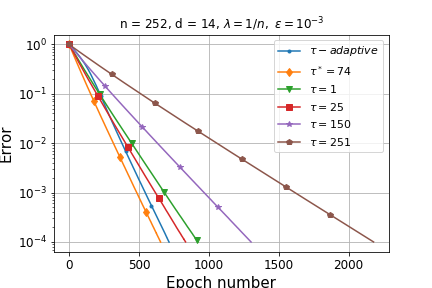
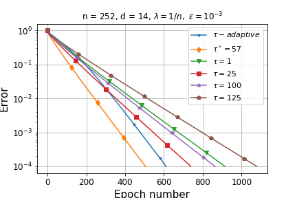
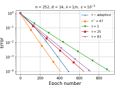
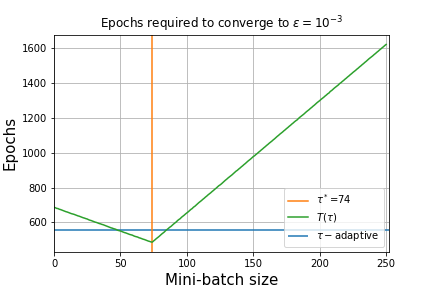
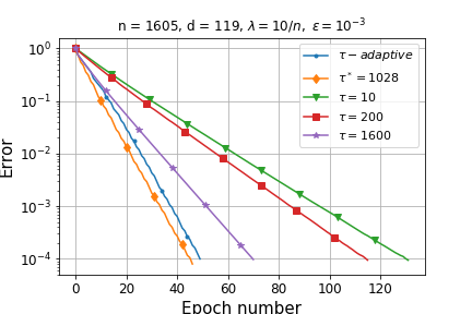
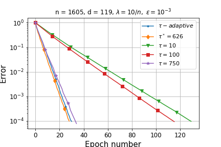
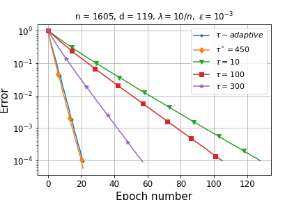
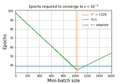
Figure 1: Convergence of ridge and logistic regression using $\tau-$partition nice sampling on bodyfat dataset (first row) and $\tau-$partition independent sampling on a1a dataset (second row).

Theorem 3.1.

Assume $f$ is $\mu-$strongly convex and assumptions 1, and 2 hold. Then the iterates of Algorithm 3 satisfy: $\mathbb{E}\left\|x^{k}-x^{*}\right\|^{2}\leq\left(1-\gamma_{\min}\mu\right)^{k}\left\|x^{0}-x^{*}\right\|^{2}+R,$

where $R=\tfrac{2\gamma_{\max}^{2}{\sigma}^{*}}{\gamma_{\min}\mu}$. Theorem 3.1 guarantees the convergence of the proposed algorithm. Although there is no significant theoretical improvement here compared to previous SGD results in the fixed batch and learning rate regimes, we measure the improvement to be significant in practice.

Convergence of ${\tau^{k}}$ to $\tau^{*}$. The motivation behind the proposed algorithm is to learn the optimal batch size in an online fashion so that we get to $\epsilon-$neighborhood of the optimal model with the minimum number of epochs. For simplicity, let’s assume that $\sigma^{*}=0$. As $x^{k}\rightarrow x^{*}$, then $h_{i}^{k}=\nabla f_{i}(x^{k})\rightarrow\nabla f_{i}(x^{*})=h_{i}^{*}$, and thus ${\tau^{k}}\rightarrow\tau^{*}$. In Theorem 3.1, we showed the convergence of $x^{k}$ to a neighborhood around $x^{*}$. Hence the theory predicts that our estimate of the optimal batch ${\tau^{k}}$ will converge to a neighborhood of the optimal batch size $\tau^{*}$.

4 Experiments

In this section, we compare our algorithm to fixed batch size SGD in terms of the number of epochs needed to reach a pre-specified neighborhood $\epsilon/10$. In the following results, we capture the convergence rate by recording the relative error $(\nicefrac{{\left\|x^{k}-x^{*}\right\|^{2}}}{{\left\|x^{0}-x^{*}\right\|^{2}}})$ where $x^{0}$ is drawn from a standard normal distribution $\mathcal{N}(0,\mathbf{I})$. We also report the number of training examples $n$, the dimension of the machine learning model $d$, regularization factor $\lambda$, and the target neighborhood $\epsilon$ above each figure. We consider the problems of regularized ridge and logistic regression where each $f_{i}$ is strongly convex and L-smooth, and $x^{*}$ can be known a-priori.Specifically, we want to $\min_{x\in\mathbb{R}^{d}}f(x)$ where

$$\vspace{-0.25cm}f_{\text{ridge}}(x)=\tfrac{1}{2n}\sum\limits_{i=1}^{n}\left\|a_{i}^{T}x-b_{i}\right\|^{2}_{2}+\tfrac{\lambda}{2}\left\|x\right\|^{2}_{2},\,\,f_{\text{logistic}}(x)=\tfrac{1}{2n}\sum\limits_{i=1}^{n}\log\left(1+\exp\left(b_{i}a_{i}^{T}x\right)\right)+\tfrac{\lambda}{2}\left\|x\right\|^{2}_{2}$$

where $(a_{i},b_{i})\sim\mathcal{D}$ are pairs of data examples from the training set. For each of the considered problems, we performed experiments on real datasets from LIBSVM Chang and Lin (2011). We tested our algorithm on ridge and logistic regression on bodyfat and a1a datasets in Figure 1. For these datasets, we considered $\tau-$partition independent and $\tau-$partition nice sampling with distributing the training set into one, two, and three partitions. Moreover, we take the previous experiments one step further by running a comparison of various fixed batch size SGD, as well as our adaptive method with a single partition (last column of 1). We plot the total iteration complexity for each batch size, and highlight optimal batch size obtained from our theoretical analysis, and how many epochs our adaptive algorithm needs to converge. This plot can be viewed as a summary of grid-search for optimal batch size (throughout all possible fixed batch sizes). Despite the fact that the optimal batch size is nontrivial and varies significantly with the model, dataset, sampling strategy, and number of partitions, our algorithm demonstrated consistent performance overall. In some cases, it was even able to cut down the number of epochs needed to reach the desired error to a factor of six.

The produced figures of our grid-search perfectly capture the tightness of our theoretical analysis. In particular, the total iteration complexity decreases linearly up to a neighborhood of $\tau^{*}$ and then increases linearly. In addition, Theorem 2.2 always captures the empirical minimum of $T(\tau)$ up to a negligible error. Moreover, these figures show how close $T_{\text{adaptive}}$ is to the total iteration complexity using optimal batch size $T(\tau^{*})$. Finally, in terms of running time, our algorithm requires $0.2322$ ms per epoch, while running SGD with the optimal batch size requires $0.2298$ ms.

5 Acknowledgement

This work was supported by the King Abdullah University of Science and Technology (KAUST) Office of Sponsored Research. The work of Motasem Alfarra and Bernard Ghanem was supported by Award No. OSR-CRG2019-4033.

Appendix A Proof of Lemma 2.1

For the considered partition sampling, the indices $1,\dots,n$ are distributed into the sets $\mathcal{C}_{1},\dots,\mathcal{C}_{K}$ with each having a minimum cardinality of $\tau$. We choose each set $\mathcal{C}_{j}$ with probability $q_{\mathcal{C}_{j}}$ where $\sum\limits_{j}q_{\mathcal{C}_{j}}=1$. Note that

$$\mathbf{P}_{ij}=\begin{cases}0&\text{if }i\in C_{k},j\in C_{l},k\neq l\\ q_{k}\frac{\tau(\tau-1)}{n_{k}(n_{k}-1)}&\text{if }i\neq j,i,j\in C_{k},|C_{k}|=\tau_{k}\\ q_{k}\frac{\tau}{n_{k}}&\text{if i=j}\end{cases}.$$

Therefore

$${\mathbb{E}}\left[\left\|\nabla f_{v}(x)-\nabla f_{v}(y)\right\|^{2}\right] = \frac{1}{n^{2}}\sum_{\mathcal{C}_{k}}\sum_{i,j\in\mathcal{C}_{k}}\frac{\mathbf{P}_{ij}}{p_{i}p_{j}}\Big{\langle}\nabla f_{i}(x)-\nabla f_{i}(y),\nabla f_{j}(x)-\nabla f_{j}(y)\Big{\rangle}$$

$$= \frac{1}{n^{2}}\sum_{\mathcal{C}_{k}}\sum_{i\neq j\in\mathcal{C}_{k}}\frac{\mathbf{P}_{ij}}{p_{i}p_{j}}\Big{\langle}\nabla f_{i}(x)-\nabla f_{i}(y),\nabla f_{j}(x)-\nabla f_{j}(y)\Big{\rangle}$$

$$+\frac{1}{n^{2}}\sum_{\mathcal{C}_{k}}\sum_{i\in\mathcal{C}_{k}}\frac{1}{p_{i}}\Big{\langle}\nabla f_{i}(x)-\nabla f_{i}(y),\nabla f_{i}(x)-\nabla f_{i}(y)\Big{\rangle}$$

$$= \frac{1}{n^{2}}\sum_{\mathcal{C}_{k}}\sum_{i\neq j\in\mathcal{C}_{k}}\frac{n_{\mathcal{C}_{k}}(\tau-1)}{q_{\mathcal{C}_{k}}\tau(n_{\mathcal{C}_{k}}-1)}\Big{\langle}\nabla f_{i}(x)-\nabla f_{i}(y),\nabla f_{j}(x)-\nabla f_{j}(y)\Big{\rangle}$$

$$+\frac{1}{n^{2}}\sum_{\mathcal{C}_{k}}\sum_{i\in\mathcal{C}_{k}}\frac{n_{\mathcal{C}_{k}}}{q_{\mathcal{C}_{k}}\tau}\Big{\langle}\nabla f_{i}(x)-\nabla f_{i}(y),\nabla f_{i}(x)-\nabla f_{i}(y)\Big{\rangle}$$

$$= \frac{1}{n^{2}}\sum_{\mathcal{C}_{k}}\frac{n_{\mathcal{C}_{k}}(\tau-1)}{q_{\mathcal{C}_{k}}\tau(n_{\mathcal{C}_{k}}-1)}\sum_{i\neq j\in\mathcal{C}_{k}}\Big{\langle}\nabla f_{i}(x)-\nabla f_{i}(y),\nabla f_{j}(x)-\nabla f_{j}(y)\Big{\rangle}$$

$$+\frac{1}{n^{2}}\sum_{\mathcal{C}_{k}}\frac{n_{\mathcal{C}_{k}}}{q_{\mathcal{C}_{k}}\tau}\sum_{i\in\mathcal{C}_{k}}\left\|\nabla f_{i}(x)-\nabla f_{i}(y)\right\|^{2}$$

$$= \frac{1}{n^{2}}\sum_{\mathcal{C}_{k}}\frac{n_{\mathcal{C}_{k}}(\tau-1)}{q_{\mathcal{C}_{k}}\tau(n_{\mathcal{C}_{k}}-1)}\left\|\sum_{i\in\mathcal{C}_{k}}\nabla f_{i}(x)-\nabla f_{i}(y)\right\|^{2}$$

$$+\frac{1}{n^{2}}\sum_{\mathcal{C}_{k}}\frac{n_{\mathcal{C}_{k}}(n_{\mathcal{C}_{k}}-\tau)}{q_{\mathcal{C}_{k}}\tau(n_{\mathcal{C}_{k}}-1)}\sum_{i\in\mathcal{C}_{k}}\left\|\nabla f_{i}(x)-\nabla f_{i}(y)\right\|^{2}$$

$$\leq \frac{1}{n^{2}}\sum_{\mathcal{C}_{k}}\frac{n_{\mathcal{C}_{k}}^{3}(\tau-1)}{q_{\mathcal{C}_{k}}\tau(n_{\mathcal{C}_{k}}-1)}2L_{\mathcal{C}_{k}}D_{f_{\mathcal{C}_{k}}}(x,y)$$

$$+\frac{1}{n^{2}}\sum_{\mathcal{C}_{k}}\frac{n_{\mathcal{C}_{k}}(n_{\mathcal{C}_{k}}-\tau)}{q_{\mathcal{C}_{k}}\tau(n_{\mathcal{C}_{k}}-1)}\sum_{i\in\mathcal{C}_{k}}2L_{i}D_{f_{i}}(x,y)$$

$$\leq \frac{1}{n^{2}}\sum_{\mathcal{C}_{k}}\frac{n_{\mathcal{C}_{k}}^{3}(\tau-1)}{q_{\mathcal{C}_{k}}\tau(n_{\mathcal{C}_{k}}-1)}2L_{\mathcal{C}_{k}}D_{f_{\mathcal{C}_{k}}}(x,y)$$

$$+\frac{1}{n^{2}}\sum_{\mathcal{C}_{k}}\frac{n_{\mathcal{C}_{k}}^{2}(n_{\mathcal{C}_{k}}-\tau)}{q_{\mathcal{C}_{k}}\tau(n_{\mathcal{C}_{k}}-1)}2\max_{i\in\mathcal{C}_{k}}{L_{i}}D_{f_{\mathcal{C}_{k}}}(x,y)$$

$$= \frac{1}{n^{2}}\sum_{\mathcal{C}_{k}}2\frac{n_{\mathcal{C}_{k}}^{2}(\tau-1)L_{\mathcal{C}_{k}}+n_{\mathcal{C}_{k}}(n_{\mathcal{C}_{k}}-\tau)\max_{i\in\mathcal{C}_{k}}{L_{i}}}{q_{\mathcal{C}_{k}}\tau(n_{\mathcal{C}_{k}}-1)}n_{\mathcal{C}_{k}}D_{f_{\mathcal{C}_{k}}}(x,y)$$

$$\leq 2\frac{1}{n}(\max_{\mathcal{C}_{k}}\frac{n_{\mathcal{C}_{k}}^{2}(\tau-1)L_{\mathcal{C}_{k}}+n_{\mathcal{C}_{k}}(n_{\mathcal{C}_{k}}-\tau)\max_{i\in\mathcal{C}_{k}}{L_{i}}}{q_{\mathcal{C}_{k}}\tau(n_{\mathcal{C}_{k}}-1)}n_{\mathcal{C}_{k}})D_{f}(x,y),$$

where $D_{f}(x,y)=f(x)-f(y)-\langle\nabla f(y),x-y\rangle$. Setting $y\leftarrow x^{*}$, leads to the desired upper bound of the expected smoothness which is given by

$$\mathcal{L}(\tau)=\frac{1}{n\tau}\left(\max_{\mathcal{C}_{k}}\frac{n_{\mathcal{C}_{k}}}{q_{\mathcal{C}_{k}}\left(n_{\mathcal{C}_{k}}-1\right)}\left(n_{\mathcal{C}_{k}}^{2}(\tau-1)L_{\mathcal{C}_{k}}+n_{\mathcal{C}_{k}}\left(n_{\mathcal{C}_{k}}-\tau\right)\max_{i\in\mathcal{C}_{k}}{L_{i}}\right)\right).$$

Next, we derive a similar bound for $\tau-$independent partition sampling.

$${\mathbb{E}}\left[\left\|\nabla f_{v}(x)-\nabla f_{v}(y)\right\|^{2}\right] = \frac{1}{n^{2}}\sum_{\mathcal{C}_{k}}\sum_{i,j\in\mathcal{C}_{k}}\frac{\mathbf{P}_{ij}}{p_{i}p_{j}}\Big{\langle}\nabla f_{i}(x)-\nabla f_{i}(y),\nabla f_{j}(x)-\nabla f_{j}(y)\Big{\rangle}$$

$$= \frac{1}{n^{2}}\sum_{\mathcal{C}_{k}}\sum_{i\neq j\in\mathcal{C}_{k}}\frac{\mathbf{P}_{ij}}{p_{i}p_{j}}\Big{\langle}\nabla f_{i}(x)-\nabla f_{i}(y),\nabla f_{j}(x)-\nabla f_{j}(y)\Big{\rangle}$$

$$+\frac{1}{n^{2}}\sum_{\mathcal{C}_{k}}\sum_{i\in\mathcal{C}_{k}}\frac{1}{p_{i}}\Big{\langle}\nabla f_{i}(x)-\nabla f_{i}(y),\nabla f_{i}(x)-\nabla f_{i}(y)\Big{\rangle}$$

$$= \frac{1}{n^{2}}\sum_{\mathcal{C}_{k}}\sum_{i\neq j\in\mathcal{C}_{k}}\frac{1}{q_{\mathcal{C}_{k}}}\Big{\langle}\nabla f_{i}(x)-\nabla f_{i}(y),\nabla f_{j}(x)-\nabla f_{j}(y)\Big{\rangle}$$

$$+\frac{1}{n^{2}}\sum_{\mathcal{C}_{k}}\sum_{i\in\mathcal{C}_{k}}\frac{1}{q_{\mathcal{C}_{k}}p_{i}}\Big{\langle}\nabla f_{i}(x)-\nabla f_{i}(y),\nabla f_{i}(x)-\nabla f_{i}(y)\Big{\rangle}$$

$$= \frac{1}{n^{2}}\sum_{\mathcal{C}_{k}}\frac{1}{q_{\mathcal{C}_{k}}}\sum_{i\neq j\in\mathcal{C}_{k}}\Big{\langle}\nabla f_{i}(x)-\nabla f_{i}(y),\nabla f_{j}(x)-\nabla f_{j}(y)\Big{\rangle}$$

$$+\frac{1}{n^{2}}\sum_{\mathcal{C}_{k}}\frac{1}{q_{\mathcal{C}_{k}}}\sum_{i\in\mathcal{C}_{k}}\frac{1}{p_{i}}\left\|\nabla f_{i}(x)-\nabla f_{i}(y)\right\|^{2}$$

$$= \frac{1}{n^{2}}\sum_{\mathcal{C}_{k}}\frac{1}{q_{\mathcal{C}_{k}}}\left\|\sum_{i\in\mathcal{C}_{k}}\nabla f_{i}(x)-\nabla f_{i}(y)\right\|^{2}$$

$$+\frac{1}{n^{2}}\sum_{\mathcal{C}_{k}}\frac{1}{q_{\mathcal{C}_{k}}}\sum_{i\in\mathcal{C}_{k}}\frac{1-p_{i}}{p_{i}}\left\|\nabla f_{i}(x)-\nabla f_{i}(y)\right\|^{2}$$

$$\leq \frac{1}{n^{2}}\sum_{\mathcal{C}_{k}}\frac{n_{\mathcal{C}_{k}}^{2}}{q_{\mathcal{C}_{k}}}2L_{\mathcal{C}_{k}}D_{f_{\mathcal{C}_{k}}}(x,y)$$

$$+\frac{1}{n^{2}}\sum_{\mathcal{C}_{k}}\frac{1}{q_{\mathcal{C}_{k}}}\sum_{i\in\mathcal{C}_{k}}\frac{1-p_{i}}{p_{i}}2L_{i}D_{f_{i}}(x,y)$$

$$\leq \frac{1}{n^{2}}\sum_{\mathcal{C}_{k}}\frac{n_{\mathcal{C}_{k}}^{2}}{q_{\mathcal{C}_{k}}}2L_{\mathcal{C}_{k}}D_{f_{\mathcal{C}_{k}}}(x,y)$$

$$+\frac{1}{n^{2}}\sum_{\mathcal{C}_{k}}\frac{n_{\mathcal{C}_{k}}}{q_{\mathcal{C}_{k}}}2\max_{i\in\mathcal{C}_{k}}\frac{1-p_{i}}{p_{i}}{L_{i}}D_{f_{\mathcal{C}_{k}}}(x,y)$$

$$= \frac{1}{n^{2}}\sum_{\mathcal{C}_{k}}2(\frac{n_{\mathcal{C}_{k}}L_{\mathcal{C}_{k}}}{q_{\mathcal{C}_{k}}}+\max_{i\in\mathcal{C}_{k}}{\frac{(1-p_{i})L_{i}}{q_{\mathcal{C}_{k}}p_{i}}})n_{\mathcal{C}_{k}}D_{f_{\mathcal{C}_{k}}}(x,y)$$

$$\leq 2\frac{1}{n}\max_{i\in\mathcal{C}_{k}}{(\frac{n_{\mathcal{C}_{k}}L_{\mathcal{C}_{k}}}{q_{\mathcal{C}_{k}}}+\max_{i\in\mathcal{C}_{k}}{\frac{(1-p_{i})L_{i}}{q_{\mathcal{C}_{k}}p_{i}})}}D_{f}(x,y).$$

This gives the desired upper bound for the expected smoothness

$$\mathcal{L}(\tau)=\frac{1}{n}\max_{i\in\mathcal{C}_{k}}{\left(\frac{n_{\mathcal{C}_{k}}L_{\mathcal{C}_{k}}}{q_{\mathcal{C}_{k}}}+\max_{i\in\mathcal{C}_{k}}\frac{(1-p_{i})L_{i}}{q_{\mathcal{C}_{k}}p_{i}}\right)}.$$

Following the same notation, we move on to compute $\sigma$ for each sampling. First, for $\tau-$nice partition sampling we have

$${\mathbb{E}}\left[\left\|\nabla f_{v}(x^{*})\right\|^{2}\right] = \frac{1}{n^{2}}\sum_{\mathcal{C}_{k}}\sum_{i,j\in\mathcal{C}_{k}}\frac{\mathbf{P}_{ij}}{p_{i}p_{j}}\Big{\langle}\nabla f_{i}(x^{*}),\nabla f_{j}(x^{*})\Big{\rangle}$$

$$= \frac{1}{n^{2}}\sum_{\mathcal{C}_{k}}\sum_{i\neq j\in\mathcal{C}_{k}}\frac{\mathbf{P}_{ij}}{p_{i}p_{j}}\Big{\langle}\nabla f_{i}(x^{*}),\nabla f_{j}(x^{*})\Big{\rangle}+\frac{1}{n^{2}}\sum_{\mathcal{C}_{k}}\sum_{i\in\mathcal{C}_{k}}\frac{1}{p_{i}}\Big{\langle}\nabla f_{i}(x^{*}),\nabla f_{i}(x^{*})\Big{\rangle}$$

$$= \frac{1}{n^{2}}\sum_{\mathcal{C}_{k}}\sum_{i\neq j\in\mathcal{C}_{k}}\frac{n_{\mathcal{C}_{k}}(\tau-1)}{\tau(n_{\mathcal{C}_{k}}-1)q_{\mathcal{C}_{k}}}\Big{\langle}\nabla f_{i}(x^{*}),\nabla f_{j}(x^{*})\Big{\rangle}+\frac{1}{n^{2}}\sum_{\mathcal{C}_{k}}\sum_{i\in\mathcal{C}_{k}}\frac{n_{\mathcal{C}_{k}}}{\tau q_{\mathcal{C}_{k}}}\Big{\langle}\nabla f_{i}(x^{*}),\nabla f_{i}(x^{*})\Big{\rangle}$$

$$= \frac{1}{n^{2}}\sum_{\mathcal{C}_{k}}\frac{n_{\mathcal{C}_{k}}(\tau-1)}{\tau(n_{\mathcal{C}_{k}}-1)q_{\mathcal{C}_{k}}}\sum_{i\neq j\in\mathcal{C}_{k}}\Big{\langle}\nabla f_{i}(x^{*}),\nabla f_{j}(x^{*})\Big{\rangle}+\frac{1}{n^{2}}\sum_{\mathcal{C}_{k}}\frac{n_{\mathcal{C}_{k}}}{\tau q_{\mathcal{C}_{k}}}\sum_{i\in\mathcal{C}_{k}}h_{i}$$

$$= \frac{1}{n^{2}}\sum_{\mathcal{C}_{k}}\frac{n_{\mathcal{C}_{k}}(\tau-1)}{\tau(n_{\mathcal{C}_{k}}-1)q_{\mathcal{C}_{k}}}\left\|\sum_{i\in\mathcal{C}_{k}}\nabla f_{i}(x^{*})\right\|^{2}+\frac{1}{n^{2}}\sum_{\mathcal{C}_{k}}\frac{n_{\mathcal{C}_{k}}(n_{\mathcal{C}_{k}}-\tau)}{\tau(n_{\mathcal{C}_{k}}-1)q_{\mathcal{C}_{k}}}\sum_{i\in\mathcal{C}_{k}}h_{i}$$

$$= \frac{1}{n^{2}}\sum_{\mathcal{C}_{k}}\frac{n_{\mathcal{C}_{k}}^{3}(\tau-1)}{\tau(n_{\mathcal{C}_{k}}-1)q_{\mathcal{C}_{k}}}{h_{\mathcal{C}_{k}}}+\frac{1}{n^{2}}\sum_{\mathcal{C}_{k}}\frac{n_{\mathcal{C}_{k}}^{2}(n_{\mathcal{C}_{k}}-\tau)}{\tau(n_{\mathcal{C}_{k}}-1)q_{\mathcal{C}_{k}}}\overline{h}_{\mathcal{C}_{k}}.$$

Where its left to rearrange the terms to get the first result of the lemma. Next, we compute $\sigma$ for $\tau-$independent partition:

$${\mathbb{E}}\left[\left\|\nabla f_{v}(x^{*})\right\|^{2}\right] = \frac{1}{n^{2}}\sum_{\mathcal{C}_{k}}\sum_{i,j\in\mathcal{C}_{k}}\frac{\mathbf{P}_{ij}}{p_{i}p_{j}}\Big{\langle}\nabla f_{i}(x^{*}),\nabla f_{j}(x^{*})\Big{\rangle}$$

$$= \frac{1}{n^{2}}\sum_{\mathcal{C}_{k}}\sum_{i\neq j\in\mathcal{C}_{k}}\frac{\mathbf{P}_{ij}}{p_{i}p_{j}}\Big{\langle}\nabla f_{i}(x^{*}),\nabla f_{j}(x^{*})\Big{\rangle}+\frac{1}{n^{2}}\sum_{\mathcal{C}_{k}}\sum_{i\in\mathcal{C}_{k}}\frac{1}{p_{i}}\Big{\langle}\nabla f_{i}(x^{*}),\nabla f_{i}(x^{*})\Big{\rangle}$$

$$= \frac{1}{n^{2}}\sum_{\mathcal{C}_{k}}\sum_{i\neq j\in\mathcal{C}_{k}}\frac{1}{q_{\mathcal{C}_{k}}}\Big{\langle}\nabla f_{i}(x^{*}),\nabla f_{j}(x^{*})\Big{\rangle}+\frac{1}{n^{2}}\sum_{\mathcal{C}_{k}}\sum_{i\in\mathcal{C}_{k}}\frac{1}{q_{\mathcal{C}_{k}}p_{i}}\Big{\langle}\nabla f_{i}(x^{*}),\nabla f_{i}(x^{*})\Big{\rangle}$$

$$= \frac{1}{n^{2}}\sum_{\mathcal{C}_{k}}\frac{1}{q_{\mathcal{C}_{k}}}\sum_{i\neq j\in\mathcal{C}_{k}}\Big{\langle}\nabla f_{i}(x^{*}),\nabla f_{j}(x^{*})\Big{\rangle}+\frac{1}{n^{2}}\sum_{\mathcal{C}_{k}}\frac{1}{q_{\mathcal{C}_{k}}}\sum_{i\in\mathcal{C}_{k}}\frac{1}{p_{i}}h_{i}$$

$$= \frac{1}{n^{2}}\sum_{\mathcal{C}_{k}}\frac{1}{q_{\mathcal{C}_{k}}}\left\|\sum_{i\in\mathcal{C}_{k}}\nabla f_{i}(x^{*})\right\|^{2}+\frac{1}{n^{2}}\sum_{\mathcal{C}_{k}}\sum_{i\in\mathcal{C}_{k}}\frac{(1-p_{i})h_{i}}{q_{\mathcal{C}_{k}}p_{i}}$$

$$= \frac{1}{n^{2}}\sum_{\mathcal{C}_{k}}\frac{n_{\mathcal{C}_{k}}^{2}}{q_{\mathcal{C}_{k}}}{h_{\mathcal{C}_{k}}}+\frac{1}{n^{2}}\sum_{\mathcal{C}_{k}}\sum_{i\in\mathcal{C}_{k}}\frac{(1-p_{i})h_{i}}{q_{\mathcal{C}_{k}}p_{i}}.$$

Appendix B Proof of Theorem 2.2

Recall that the optimal batch size $\tau(x^{*})$ is chosen such that the quantity $\max\left\{\tau\mathcal{L}(\tau),\tfrac{2}{\epsilon\mu}\tau\sigma(x^{*},\tau)\right\}$ is minimized. Note that in both $\tau-$nice partition, and $\tau-$ independent partition with $(p_{i}=\tfrac{\tau}{n_{\mathcal{C}_{j}}})$, $\tau\sigma(x^{*},\tau)$ is a linear function of $\tau$ while $\tau\mathcal{L}(\tau)$ is a max across linearly increasing functions of $\tau$. To find the minimized in such a case, we leverage the following lemma.

Lemma B.1.

Suppose that $l_{1}(x),l_{2}(x),...,l_{k}(x)$ are increasing linear functions of $x$, and $r(x)$ is linear decreasing function of $x$, then the minimizer of $\max(l_{1}(x),l_{2}(x),...,l_{k}(x),r(x))$ is $x^{*}=\min_{i}(x_{i})$ where $x_{i}$ is the unique solution for $l_{i}(x)=r(x)$

Proof: Let $x^{*}$ be defined as above, and let $x$ be an arbitrary number. If $x\leq x^{*}$, then $r(x)\geq r(x^{*})\geq r(x_{i})=l_{i}(x_{i})\geq l_{i}(x^{*})$ for each $i$ which means $r(x)\geq\max(l_{1}(x^{*}),...,l_{k}(x^{*}),r(x^{*}))$. On the other hand, if $x\geq x^{*}$, then let $i$ be the index s.t. $x_{i}=x^{*}$. We have $l_{i}(x)\geq l_{i}(x^{*})=r(x^{*})\geq r(x_{j})=l_{j}(x_{j})\geq l_{j}(x^{*})$, hence $l_{i}(x)\geq\max(l_{1}(x^{*}),...,l_{k}(x^{*}),r(x^{*}))$. This means that $x^{*}=\min_{i}(x_{i})$ is indeed the minimizer of $\max(l_{1}(x),l_{2}(x),...,l_{k}(x),r(x))$.

Now we can estimate optimal batch sizes for proposed samplings.

$\tau-$nice partition: if $\sum_{\mathcal{C}_{j}}\tfrac{n_{\mathcal{C}_{j}}^{2}}{e_{j}}(h_{\mathcal{C}_{j}}^{*}n_{\mathcal{C}_{j}}-\overline{h}^{*}_{\mathcal{C}_{j}})\leq 0$ then $\tau\sigma(\tau)$ is a decreasing linear function of $\tau$, and $\tau\mathcal{L}(\tau)$ is the max of increasing linear functions. Therefore, we can leverage the previous lemma with $r(\tau)=\frac{2}{\epsilon\mu}\tau\sigma(x^{*},\tau)$ and $l_{\mathcal{C}_{k}}(\tau)=\frac{n_{\mathcal{C}_{k}}^{2}(\tau-1)L_{\mathcal{C}_{k}}+n_{\mathcal{C}_{k}}(n_{\mathcal{C}_{k}}-\tau)\max_{i\in\mathcal{C}_{k}}{L_{i}}}{q_{\mathcal{C}_{k}}(n_{\mathcal{C}_{k}}-1)}n_{\mathcal{C}_{k}}$ to find the optimal batch size as $\tau^{*}=\min\limits_{\mathcal{C}_{k}}(\tau^{*}_{\mathcal{C}_{k}})$, where

$$\tau^{*}_{\mathcal{C}_{k}}=\tfrac{\tfrac{nn_{\mathcal{C}_{r}}^{2}}{e_{\mathcal{C}_{r}}}(L_{\mathcal{C}_{r}}-L_{\max}^{\mathcal{C}_{r}})+\tfrac{2}{\epsilon\mu}\sum_{\mathcal{C}_{j}}\tfrac{n_{\mathcal{C}_{j}}^{3}}{e_{\mathcal{C}_{j}}}\left(\overline{h}_{\mathcal{C}_{j}}-h_{\mathcal{C}_{j}}\right)}{\tfrac{nn_{\mathcal{C}_{r}}}{e_{\mathcal{C}_{r}}}(n_{\mathcal{C}_{r}}L_{\mathcal{C}_{r}}-L_{\max}^{\mathcal{C}_{r}})+\tfrac{2}{\epsilon\mu}\sum_{\mathcal{C}_{j}}\tfrac{n_{\mathcal{C}_{j}}^{2}}{e_{\mathcal{C}_{j}}}({\overline{h}_{\mathcal{C}_{j}}-n_{\mathcal{C}_{j}}h_{\mathcal{C}_{j}}})}.$$

$\tau-$independent partition: Similar to $\tau-$nice partition, we have $\tau\sigma(\tau)$ is a decreasing linear function of $\tau$ if $\quad\sum_{\mathcal{C}_{j}}\tfrac{n_{\mathcal{C}_{j}}}{q_{\mathcal{C}_{j}}}(n_{\mathcal{C}_{j}}h_{\mathcal{C}_{j}}^{*}-\overline{h}^{*}_{\mathcal{C}_{j}})\leq 0$, and $\tau\mathcal{L}(\tau)$ is the max of increasing linear functions of $\tau$. Hence, we can leverage the previous lemma with $r(\tau)=\frac{2}{\epsilon\mu}\tau\sigma(x^{*},\tau)$ and $l_{\mathcal{C}_{k}}(\tau)={\frac{n_{\mathcal{C}_{k}}L_{\mathcal{C}_{k}}\tau}{q_{\mathcal{C}_{k}}}+(n_{\mathcal{C}_{k}}-\tau)\max_{i\in\mathcal{C}_{k}}{\frac{L_{i}}{q_{\mathcal{C}_{k}}}}}$ to find the optimal batch size as $\tau^{*}=\min\limits_{\mathcal{C}_{k}}(\tau^{*}_{\mathcal{C}_{k}})$, where

$$\tau^{*}_{\mathcal{C}_{k}}={\tfrac{\tfrac{2}{\epsilon\mu}\sum_{\mathcal{C}_{j}}\tfrac{n_{\mathcal{C}_{j}}^{2}}{q_{\mathcal{C}_{j}}}\overline{h}_{\mathcal{C}_{j}}-\tfrac{n}{q_{\mathcal{C}_{r}}}L_{\max}^{\mathcal{C}_{r}}}{\tfrac{2}{\epsilon\mu}\sum_{\mathcal{C}_{j}}\tfrac{n_{\mathcal{C}_{j}}}{q_{\mathcal{C}_{j}}}(\overline{h}_{\mathcal{C}_{j}}-n_{\mathcal{C}_{j}}h_{\mathcal{C}_{j}})+\tfrac{n}{q_{\mathcal{C}_{r}}}(n_{\mathcal{C}_{r}}L_{\mathcal{C}_{r}}-L_{\max}^{\mathcal{C}_{r}})}}.$$

Appendix C Proof of bounds on step sizes

For our choice of the learning rate we have

$$\gamma^{k}=\frac{1}{2}\min\left\{\frac{1}{{\mathcal{L}^{k}}},\frac{\epsilon\mu}{\min(C,2{\sigma}^{k})}\right\}=\frac{1}{2}\min\left\{\frac{1}{{\mathcal{L}^{k}}},\max\left\{\frac{\epsilon\mu}{C},\frac{\epsilon\mu}{2{\sigma}^{k}}\right\}\right\}\geq\frac{1}{2}\min\left\{\frac{1}{{\mathcal{L}^{k}}},\frac{\epsilon\mu}{C}\right\}.$$

Since ${\mathcal{L}^{k}}$ is a linear combination between the smoothness constants of the functions $f_{i}$, then it is bounded. Therefore, both ${\mathcal{L}^{k}}$ and $C$ are upper bounded and lower bounded as well as $\frac{1}{{\mathcal{L}^{k}}}$ and $\frac{\epsilon\mu}{C}$, thus also $\gamma^{k}$ is bounded by positive constants $\gamma_{\max}=\tfrac{1}{2}\max_{\tau\in[n]}\left\{\tfrac{1}{\mathcal{L}(\tau)}\right\}$ and $\gamma_{\min}=\frac{1}{2}\min\left\{\min_{\tau\in[n]}\left\{\tfrac{1}{\mathcal{L}(\tau)}\right\},\tfrac{\epsilon\mu}{C}\right\}$.

Appendix D Proof of Theorem 3.1

Let $r^{k}=\left\|x^{k}-x^{*}\right\|^{2}$, then

$${\mathbb{E}}\left[r^{k+1}|x^{k}\right] = {\mathbb{E}}\left[\left\|x^{k}-\gamma^{k}\nabla f_{v_{k}}(x^{k})-x^{*}\right\|^{2}|x^{k}\right]$$

$$= r^{k}+(\gamma^{k})^{2}{\mathbb{E}}\left[\left\|\nabla f_{v_{k}}(x^{k})\right\|^{2}|x^{k}\right]-2\gamma^{k}\langle{\mathbb{E}}\left[\nabla f_{v_{k}}(x^{k})|x^{k}\right],r^{k}\rangle$$

$$= r^{k}+(\gamma^{k})^{2}{\mathbb{E}}\left[\left\|\nabla f_{v_{k}}(x^{k})\right\|^{2}|x^{k}\right]-2\gamma^{k}\left(f(x^{k})-f(x^{*})+\frac{\mu}{2}r^{k}\right)$$

$$= (1-\gamma^{k}\mu)r^{k}+(\gamma^{k})^{2}{\mathbb{E}}\left[\left\|\nabla f_{v_{k}}(x^{k})\right\|^{2}|x^{k}\right]-2\gamma^{k}(f(x^{k})-f(x^{*}))$$

$$\leq (1-\gamma^{k}\mu)r^{k}+(\gamma^{k})^{2}(4\mathcal{L}^{k}(f(x^{k})-f(x^{*}))+2{\sigma})-2\gamma^{k}(f(x^{k})-f(x^{*}))$$

$$= (1-\gamma^{k}\mu)r^{k}-2\gamma^{k}((1-2\gamma^{k}\mathcal{L}^{k})(f(x^{k})-f(x^{*})))+2(\gamma^{k})^{2}{\sigma}$$

$$\leq (1-\gamma^{k}\mu)r^{k}+2(\gamma^{k})^{2}{\sigma}\quad\text{ for }\gamma_{k}\leq\frac{1}{2\mathcal{L}^{k}}.$$

From Eariler bounds, there exist upper and lower bounds for step-sizes, $\gamma_{\min}\leq\gamma^{k}\leq\gamma_{\max}$, thus

$${\mathbb{E}}\left[r^{k+1}|x^{k}\right]\leq(1-\gamma^{k}\mu)r^{k}+2(\gamma^{k})^{2}{\sigma}\leq(1-\gamma_{\min}\mu)r^{k}+2\gamma_{\max}^{2}{\sigma}.$$

Therefore, unrolling the above recursion gives

$${\mathbb{E}}\left[r^{k+1}|x^{k}\right] \leq (1-\gamma_{\min}\mu)^{k}r^{0}+2\gamma_{\max}^{2}{\sigma}\sum_{i=0}^{k}(1-\gamma_{\min}\mu)^{k}$$

$$\leq (1-\gamma_{\text{min}}\mu)^{k}r^{0}+\frac{2\gamma_{\max}^{2}{\sigma}}{\gamma_{\text{min}}\mu}.$$

Appendix E Proof of convergence to linear neighborhood in $\epsilon$

In this section, we prove that our algorithm converges to a neighborhood around the optimal solution with size upper bounded by an expression linear in $\epsilon$. First of all, we prove that ${\sigma}(x)$ is lower bounded by a multiple of the variance in the optimum ${\sigma}^{*}$ (in Lemma E.1). Then, by showing an alternative upper bound on the step-size, we obtain an upper bound for neighborhood size $R$ as expression of $\epsilon$.

Lemma E.1.

Suppose $f$ is $\mu-$strongly convex, $L-$smooth and with expected smoothness constant $\mathcal{L}$. Let $v$ be as in the SGD overview, i.e., ${\mathbb{E}}\left[v_{i}=1\right]$ for all $i$. Fix any $c>0$. The function $\sigma(x)={\mathbb{E}}\left[\left\|\nabla{f_{v}(x)}\right\|^{2}\right]$ can be lower bounded as follows:

$$\sigma(x)\geq\left\{\mu^{2}c,1-2\sqrt{\mathcal{L}Lc}\right\}\sigma(x^{*}),\qquad\forall x\in\mathbb{R}^{d}.$$

The constant $c$ maximizing this bound is $c=\left(\frac{\sqrt{\mathcal{L}L+\mu^{2}}-\sqrt{\mathcal{L}L}}{\mu^{2}}\right)^{2}$, giving the bound

$$\sigma(x)\geq\frac{\left(\sqrt{\mathcal{L}L+\mu^{2}}-\sqrt{\mathcal{L}L}\right)^{2}}{\mu^{2}}\sigma(x^{*}),\qquad\forall x\in\mathbb{R}^{d}.$$

Proof: Choose $c>0$. If $\left\|x-x^{*}\right\|\geq\sqrt{c\sigma(x^{*})}$, then using Jensen’s inequality and strong convexity of $f$, we get

$$\sigma(x)\geq\left\|{\mathbb{E}}\left[\nabla{f_{v}(x)}\right]\right\|^{2}=\left\|\nabla{f(x)}\right\|^{2}=\left\|\nabla{f(x)}-\nabla{f(x^{*})}\right\|^{2}\geq\mu^{2}\left\|x-x^{*}\right\|^{2}\geq\mu^{2}c\sigma(x^{*}).$$ (3)

If $\left\|x-x^{*}\right\|\leq\sqrt{c\sigma(x^{*})}$, then using expected smoothness and $L$-smoothness, we get

$${\mathbb{E}}\left[\left\|\nabla{f_{v}(x)}-\nabla{f_{v}(x^{*})}\right\|^{2}\right]\overset{\eqref{eq:exp_smoothn_cL}}{\leq}2\mathcal{L}(f(x)-f(x^{*}))\leq\mathcal{L}L\left\|x-x^{*}\right\|^{2}\leq\mathcal{L}Lc\sigma(x^{*}).$$ (4)

Further, we can write

$$\sigma(x^{*})-\sigma(x) = {\mathbb{E}}\left[\left\|\nabla{f_{v}(x^{*})}\right\|^{2}\right]-{\mathbb{E}}\left[\left\|\nabla{f_{v}(x)}\right\|^{2}\right]$$

$$= -2{\mathbb{E}}\left[\left\langle\nabla{f_{v}(x)}-\nabla{f_{v}(x^{*})},\nabla{f_{v}(x^{*})}\right\rangle\right]-{\mathbb{E}}\left[\left\|\nabla{f_{v}(x)}-\nabla{f_{v}(x^{*})}\right\|^{2}\right]$$

$$\leq -2{\mathbb{E}}\left[\left\langle\nabla{f_{v}(x)}-\nabla{f_{v}(x^{*})},\nabla{f_{v}(x^{*})}\right\rangle\right]$$

$$\leq 2{\mathbb{E}}\left[\left\|\nabla{f_{v}(x)}-\nabla{f_{v}(x^{*})}\right\|\left\|\nabla{f_{v}(x^{*})}\right\|\right]$$

$$\leq 2\sqrt{{\mathbb{E}}\left[\left\|\nabla{f_{v}(x)}-\nabla{f_{v}(x^{*})}\right\|^{2}\right]}\sqrt{{\mathbb{E}}\left[\left\|\nabla{f_{v}(x^{*})}\right\|^{2}\right]}$$

$$\overset{\eqref{eqL:bui7gd97dd}}{\leq} 2\sqrt{\mathcal{L}Lc}\sqrt{\sigma(x^{*})}\sqrt{\sigma(x^{*})}$$

$$= 2\sqrt{\mathcal{L}Lc}\sigma(x^{*}),$$

where the first inequality follows by neglecting a negative term, the second by Cauchy-Schwarz and the third by Hölder inequality for bounding the expectation of the product of two random variables. The last inequality implies that

$$\sigma(x)\geq\left(1-2\sqrt{\mathcal{L}Lc}\right)\sigma(x^{*}).$$ (5)

By combining the bounds (3) and (5), we get

$$\sigma(x)\geq\min\left\{\mu^{2}c,1-2\sqrt{\mathcal{L}Lc}\right\}\sigma(x^{*}).$$

Using Lemma E.1, we can upper bound step-sizes $\gamma^{k}$. Assume that $\sigma^{*}=\sigma(x^{*})>0$. Let $\gamma_{\max}^{{}^{\prime}}=\frac{\epsilon\mu}{2}\max\left\{\frac{1}{C},\frac{1}{2\eta{\sigma}^{*}}\right\}$, where $\eta=\frac{\left(\sqrt{\mathcal{L}L+\mu^{2}}-\sqrt{\mathcal{L}L}\right)^{2}}{\mu^{2}}$.

We have

$$\gamma^{k}=\frac{1}{2}\min\left\{\frac{1}{{\mathcal{L}^{k}}},\frac{\epsilon\mu}{\min(C,2{\sigma}^{k})}\right\}\leq\frac{\epsilon\mu}{2}\max\left\{\frac{1}{C},\frac{1}{2{\sigma}^{k}}\right\}\leq\frac{\epsilon\mu}{2}\max\left\{\frac{1}{C},\frac{1}{2\eta{\sigma}^{*}}\right\}=\gamma_{\max}^{{}^{\prime}}.$$

Now, we use this alternative step-sizes upper bound to obtain alternative expression for residual term $R=\frac{2\gamma^{2}_{\max}{\sigma}^{*}}{\gamma_{\text{min}}\mu}$ in Theorem 3.1 (let’s denote it $R^{{}^{\prime}}$). Analogically to proof of Theorem 3.1 (with upper bound of step-sizes $\gamma_{\max}^{{}^{\prime}}$), we have $R^{{}^{\prime}}=\frac{2\gamma^{{}^{\prime}2}_{\max}{\sigma}^{*}}{\gamma_{\text{min}}\mu}$.

Finally, expanding expression for residual term $R^{{}^{\prime}}$ yields the result:

$$R^{{}^{\prime}} =\frac{2\gamma^{{}^{\prime}2}_{\max}{\sigma}^{*}}{\gamma_{\text{min}}\mu}=\frac{2\left(\frac{\epsilon\mu}{2}\max\left\{\frac{1}{C},\frac{1}{2\eta{\sigma}^{*}}\right\}\right)^{2}{\sigma}^{*}}{\frac{1}{2}\min\left\{\min_{\tau\in[n]}\left\{\tfrac{1}{\mathcal{L}(\tau)}\right\},\tfrac{\epsilon\mu}{C}\right\}\mu}=\epsilon^{2}\mu\left(\max\left\{\frac{1}{C},\frac{1}{2\eta{\sigma}^{*}}\right\}\right)^{2}\max\left\{\max_{\tau\in[n]}\left\{\mathcal{L}(\tau)\right\},\tfrac{C}{\mu\epsilon}\right\}{\sigma}^{*}$$

$$=\epsilon\mu\left(\max\left\{\frac{1}{C},\frac{1}{2\eta{\sigma}^{*}}\right\}\right)^{2}\max\left\{\epsilon\max_{\tau\in[n]}\left\{\mathcal{L}(\tau)\right\},\tfrac{C}{\mu}\right\}{\sigma}^{*}.$$

As conclusion, if we consider $R^{{}^{\prime}}$ to be function of $\epsilon$, then it is at least linear in $\epsilon$, $R^{{}^{\prime}}\in\mathcal{O}(\epsilon)$.

Appendix F Additional Experimental Results

In this section, we present additional experimental results. Here we test each dataset on the sampling that was not tested on. Similar to the earlier result, the proposed algorithm outperforms most of the fixed batch size SGD. Moreover, it can be seen as a first glance, that the optimal batch is non-trivial, and it is changing as we partition the dataset through different number of partitions. For example, in bodyfat dataset that is located in one partition, the optimal batch size was $\tau^{*}=74$. Although one can still sample $\tau=74$ when the data is divided into two partitions, the optimal has changed to $\tau^{*}=57$. This is clearly shown in Figure 4 where it shows that the optimal batch size varies between different partitioning, and the predicted optimal from our theoretical analysis matches the actual optimal.

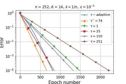
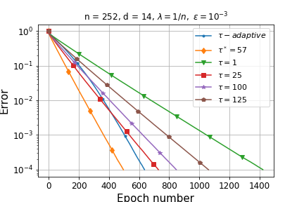
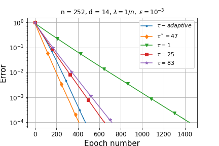
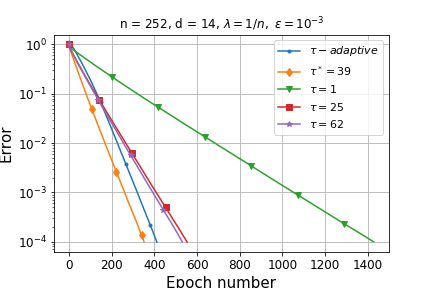
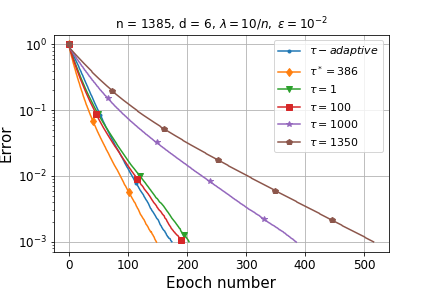
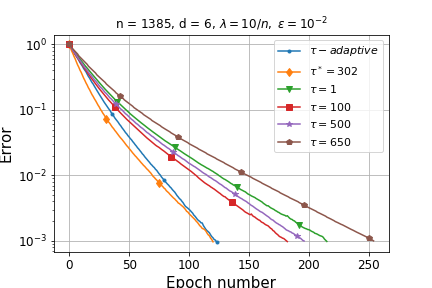
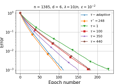
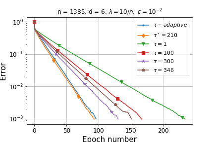
Figure 2: Convergence of Ridge regression using $\tau-$partition independent sampling on Bodyfat dataset (first row) and $\tau-$partition nice sampling on mg dataset (second row). In first three columns, training set is distributed among $1$, $2$, $3$ and $4$ partitions, respectively.

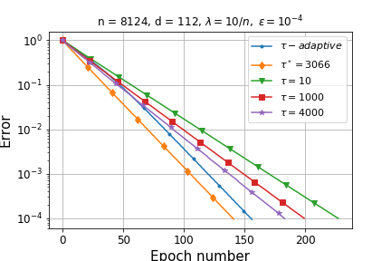
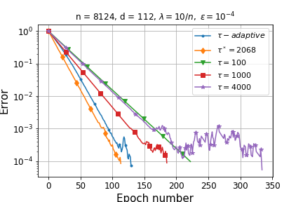
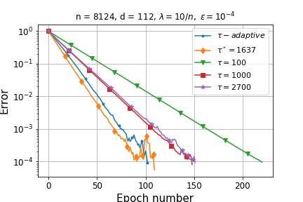
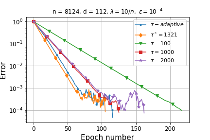
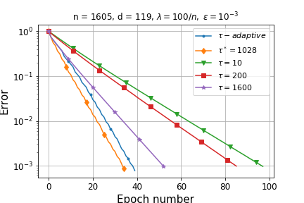
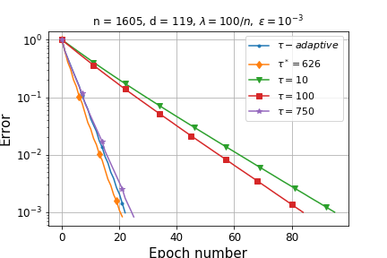
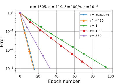
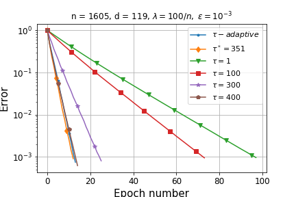
Figure 3: Convergence of Logistic regression using $\tau-$partition independent sampling on mushrooms dataset (first row) and $\tau-$partition nice sampling on a1a dataset (second row). In first three columns, training set is distributed among $1$, $2$, $3$ and $4$ partitions, respectively.

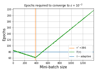
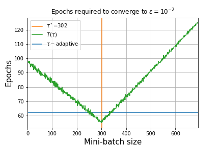
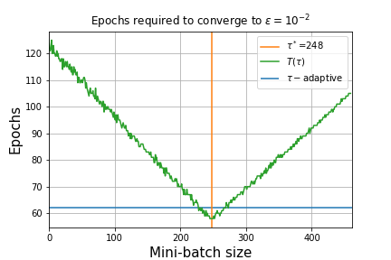
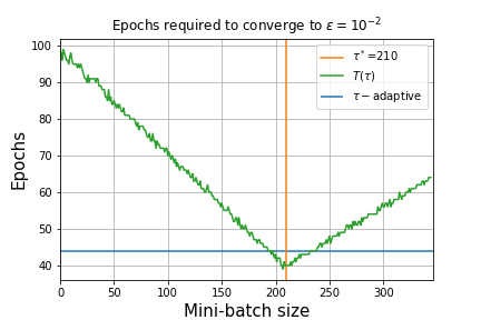
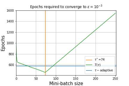
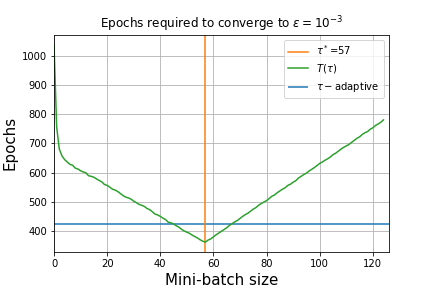
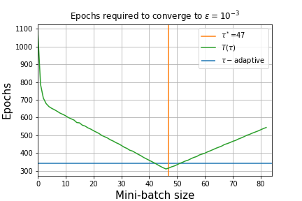
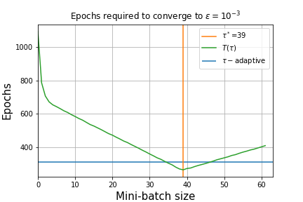
Figure 4: Effect of batch size on the total iteration complexity. First row: mg dataset sampled using $\tau-$nice partition sampling. Second row: bodyfat dataset sampled using $\tau-$independent partition sampling. From left to right: dataset is distributed across $1$, $2$, $3$, and $4$ partitions. This figure reflects the tightness of the theoretical result in relating the total iteration complexity with the batch size, and the optimal batch size. Moreover, This figure shows how close the proposed algorithm is to the optimal batch size in terms of the performance.

References

- Barzilai and Borwein (1988) Jonathan Barzilai and Jonathan M Borwein. Two-point Step Size Gradient Methods. IMA Journal of Numerical Analysis, 8(1):141–148, 1988.
- Bottou (2010) Léon Bottou. Large-scale Machine Learning with Stochastic Gradient Descent. In Proceedings of COMPSTAT’2010, pages 177–186. Springer, 2010.
- Chang and Lin (2011) Chih-Chung Chang and Chih-Jen Lin. LIBSVM: A library for Support Vector Machines. ACM Transactions on Intelligent Systems and Technology (TIST), 2(3):1–27, 2011.
- De et al. (2017) Soham De, Abhay Yadav, David Jacobs, and Tom Goldstein. Automated Inference with Adaptive Batches. In Proceedings of the 20th International Conference on Artificial Intelligence and Statistics, pages 1504–1513, 2017.
- Masters and Luschi (2018) Dominic Masters and Carlo Luschi. Revisiting Small Batch Training for Deep Neural Networks. arXiv preprint arXiv:1804.07612, 2018.
- Mathews and Xie (1993) V John Mathews and Zhenhua Xie. A Stochastic Gradient Adaptive Filter with Gradient Adaptive Step Size. IEEE transactions on Signal Processing, 41(6):2075–2087, 1993.
- Nemirovski et al. (2009) Arkadi Nemirovski, Anatoli Juditsky, Guanghui Lan, and Alexander Shapiro. Robust Stochastic Approximation Approach to Stochastic Programming. SIAM Journal on Optimization, 19(4):1574–1609, 2009.
- Qian et al. (2019) Xun Qian, Peter Richtárik, Robert M. Gower, Alibek Sailanbayev, Nicolas Loizou, and Egor Shulgin. SGD with arbitrary sampling: General analysis and improved rates. In Proceedings of the 36th International Conference on Machine Learning, ICML 2019, 9-15, 2019.
- Robbins and Monro (1951) Herbert Robbins and Sutton Monro. A Stochastic Approximation Method. The Annals of Mathematical Statistics, pages 400–407, 1951.
- Schumer and Steiglitz (1968) MA Schumer and Kenneth Steiglitz. Adaptive Step Size Random Search. IEEE Transactions on Automatic Control, 13(3):270–276, 1968.
- Shin et al. (2017) Sungho Shin, Yoonho Boo, and Wonyong Sung. Fixed-Point Optimization of Deep Neural Networks with Adaptive Step Size Retraining. In 2017 IEEE International Conference on Acoustics, Speech and Signal Processing (ICASSP), pages 1203–1207. IEEE, 2017.
- Smith et al. (2019) Samuel L. Smith, Pieter-Jan Kindermans, and Quoc V. Le. Don’t decay the learning rate, increase the batch size. In International Conference on Learning Representations, 2019.
- Tan et al. (2016) Conghui Tan, Shiqian Ma, Yu-Hong Dai, and Yuqiu Qian. Barzilai-Borwein Step Size for Stochastic Gradient Descent. In Advances in Neural Information Processing Systems, pages 685–693, 2016.
- You et al. (2017a) Yang You, Igor Gitman, and Boris Ginsburg. Large Batch Training of Convolutional Networks. arXiv preprint arXiv:1708.03888, 2017a.
- You et al. (2017b) Yang You, Igor Gitman, and Boris Ginsburg. Scaling SGD Batch Size to 32k for Imagenet Training. arXiv preprint arXiv:1708.03888, 6, 2017b.
- Zeiler (2012) Matthew D Zeiler. ADADELTA: an adaptive learning rate method. arXiv preprint arXiv:1212.5701, 2012.