Local analysis of a two phase free boundary problem concerning mean curvature

Abstract

We consider an overdetermined problem for a two phase elliptic operator in divergence form with piecewise constant coefficients. We look for domains such that the solution $u$ of a Dirichlet boundary value problem also satisfies the additional property that its normal derivative $\partial_{n}u$ is a multiple of the radius of curvature at each point on the boundary. When the coefficients satisfy some “non-criticality” condition, we construct nontrivial solutions to this overdetermined problem employing a perturbation argument relying on shape derivatives and the implicit function theorem. Moreover, in the critical case, we employ the use of the Crandall-Rabinowitz theorem to show the existence of a branch of symmetry breaking solutions bifurcating from trivial ones. Finally, some remarks on the one phase case and a similar overdetermined problem of Serrin type are given.

Key words. two-phase, overdetermined problem, free boundary problem, mean curvature, implicit function theorem, Crandall-Rabinowitz theorem, bifurcation.

AMS subject classifications. 35N25, 35J15, 34K18, 35Q93.

1 Introduction

1.1 Problem setting and known results

Let $\Omega\subset{\mathbb{R}}^{N}$ ($N\geq 2$) be a bounded domain of class $\mathcal{C}^{2}$ and $D\subset\overline{D}\subset\Omega$ be an open set of class $\mathcal{C}^{2}$ with at most finitely many connected components such that $\Omega\setminus D$ is connected. Moreover, let $n$ denote the outward unit normal vector to both $\partial\Omega$ and $\partial D$ and let their mean curvature $H$ be defined as the tangential divergence of the normal vector $n$, that is $\mathop{\mathrm{div}}_{\tau}(n)$ (notice that, under this definition, the mean curvature of a ball of radius $R$ is equal to $(N-1)/R$ everywhere on the boundary). Given a positive constant $\sigma_{c}\neq 1$, define the following piecewise constant function:

$$\sigma(x)=\sigma_{c}\ \mathcal{X}_{D}+\mathcal{X}_{\Omega\setminus D},$$ (1.1)

where $\mathcal{X}_{A}$ is the characteristic function of the set $A$ (i.e., $\mathcal{X}_{A}(x)$ is $1$ if $x\in A$ and $0$ otherwise). The aim of this paper is to study the following two phase overdetermined problem. Find those pairs of domains $(D,\Omega)$ with the properties stated in the introduction such that the mean curvature $H$ of $\partial\Omega$ never vanishes and such that the following overdetermined problem admits a solution for some real constant $d>0$.

$$-\mathop{\mathrm{div}}\left(\sigma\nabla u\right)=1\quad\text{in }\Omega,$$ (1.2)

$$u=0\quad\text{on }\partial\Omega,$$ (1.3)

$$\partial_{n}u=-d/H\quad\text{on }\partial\Omega,$$ (1.4)

where $\partial_{n}$ stands for the outward normal derivative at the boundary.

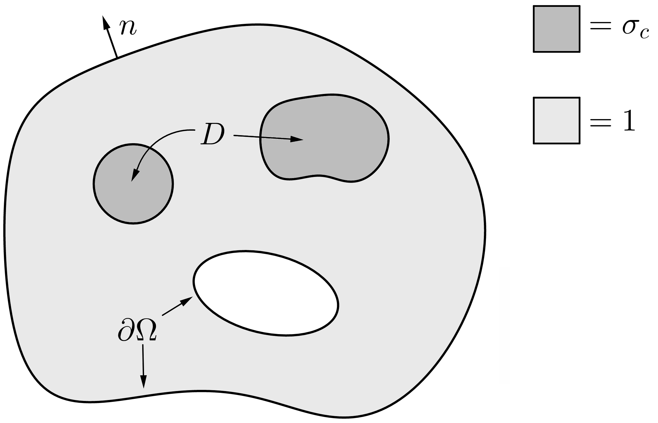
Figure 1: Problem setting

One of the most famous (and influential) results concerning one phase overdetermined problems is due to Serrin [Se]. In particular, he showed that balls are the only domains such that the value $u(x)$ and the normal derivative $\partial_{n}u(x)$ of the solution $u$ of some given elliptic problem (for the Laplace operator) both attain a constant value on the boundary (see Theorem 6.1, later in this paper). Many mathematicians, inspired by Serrin’s theorem, have extended his results and given alternative proofs: we refer the interested reader to the survey papers [Ma, NT] and the references therein. In particular, similar overdetermined problems corresponding to nonconstant overdetermined conditions (such as [BHS]) and the corresponding stability properties have been considered (see [BNST, MP1, MP2, MP3]).

On the other hand, two phase overdetermined problems (that is, overdetermined problems related to an operator in divergence form like the one in (1.2)) show a more diverse behavior. Indeed, depending on the setting, the solutions of such overdetermined problems might enjoy a high degree of symmetry just as in Serrin’s original work (see [KLeS, Sak1, Sak2, CMS, Sak3, CSU]) or allow for the existence of nontrivial (nonsymmetric) solutions, due to the interaction between the geometry of the two phases $D$ and $\Omega\setminus D$ (see [KLiS, CMS, CY1, CY2]).

1.2 Main results for overdetermined problem (1.2)–(1.4)

Overdetermined problem (1.2)–(1.4) has the following interpretation. If one considers $\sigma_{c}$ to be a dimensionless quantity, then, a quick dimensional analysis yields that the solution $u$ of the boundary value problem (1.2)–(1.3) has the dimension of length squared. As a consequence, its normal derivative $\partial_{n}u$ has the dimension of length. Overdetermined condition (1.4) then translates to requiring that the value $\partial_{n}u(x)$ be directly proportional to the radius of curvature at each point $x\in\partial\Omega$.

First of all, it is important to notice that, unlike the boundary value problem (1.2)–(1.3), the overdetermined problem (1.2)–(1.4) is not solvable for all pairs $(D,\Omega)$. In what follows, when no confusion arises, we will also refer to the very pairs of domains $(D,\Omega)$ that make problem (1.2)–(1.4) solvable as solutions of (1.2)–(1.4). In particular, notice that, for all values of $\sigma_{c}>0$, any pair of concentric balls $(D_{0},\Omega_{0})$ is a solution of (1.2)–(1.4) corresponding to $d=\frac{N-1}{N}$. We will refer to such pairs as trivial solutions. By a scaling argument, it is enough to check this fact when $\Omega_{0}$ is the unit ball centered at the origin and $D_{0}$ is the concentric ball with radius $0<R<1$. Under these assumptions, the unique solution to (1.2)–(1.3) is given by

$$u(x)=\begin{cases}\displaystyle\frac{1-R^{2}}{2N}+\frac{R^{2}-|x|^{2}}{2N\sigma_{c}}&\quad|x|\in[0,R),\\ \vspace*{-6mm}\\ \displaystyle\frac{1-|x|^{2}}{2N}&\quad|x|\in[R,1],\end{cases}$$ (1.5)

and also satisfies the overdetermined condition (1.4) for $d=\frac{N-1}{N}$.

Notice that the limit case $R=0$ in the above corresponds to the pair $(\emptyset,\Omega_{0})$, which, for the purpose of this paper, will still be considered a trivial solution of (1.2)–(1.4).

Theorem I.

Problem (1.2)–(1.4) has no solution if $d>\frac{N-1}{N}$. Moreover, if $d=\frac{N-1}{N}$ then the only solutions of (1.2)–(1.4) are trivial.

The one phase analogue of overdetermined problem (1.2)–(1.4) in the critical case $d=\frac{N-1}{N}$ was studied by Magnanini and Poggesi in [MP2]. The authors also showed stability estimates by means of integral inequalities.

In what follows, we will let the quantity $d\leq\frac{N-1}{N}$ vary and study the nontrivial solutions of problem (1.2)–(1.4) that are obtained by a small perturbation of trivial ones. Let $(D_{0},\Omega_{0})$ denote a pair of concentric balls centered at the origin. In what follows, pairs of perturbed domains, denoted by $(D_{f},\Omega_{g})$, will be parametrized by functions $f\in\mathcal{F}$, $g\in{\mathcal{G}}$, where

$$\mathcal{F}=\left\{f\in\mathcal{C}^{2,\alpha}(\partial D_{0})\;\mathrel{\mathop{\mathchar 58\relax}}\;\int_{\partial D_{0}}f=0\right\}\quad\text{and}\quad{\mathcal{G}}=\left\{g\in\mathcal{C}^{2,\alpha}(\partial\Omega_{0})\;\mathrel{\mathop{\mathchar 58\relax}}\;\int_{\partial\Omega_{0}}g=0\right\}.$$ (1.6)

If the functions $f$ and $g$ are sufficiently small, the perturbed domains $D_{f}$ and $\Omega_{g}$ are well defined as the unique bounded domains whose boundaries are

$$\partial D_{f}=\Big{\{}x+f(x)n(x)\;\mathrel{\mathop{\mathchar 58\relax}}\;x\in\partial D_{0}\Big{\}}\quad\text{and}\quad\partial\Omega_{g}=\Big{\{}x+g(x)n(x)\;\mathrel{\mathop{\mathchar 58\relax}}\;x\in\partial\Omega_{0}\Big{\}}.$$ (1.7)

In order to study the nontrivial solutions of (1.2)–(1.4), we will employ the use of a mapping

$$\mathcal{F}\times{\mathcal{G}}\times(0,\infty)\ni(f,g,s)\mapsto\Phi(f,g,s)$$

that vanishes if and only if the pair $(D_{f},\Omega_{g})$ is a solution to problem (1.2)–(1.4) when $\sigma_{c}=s$. The precise definition of $\Phi$ will be given in (3.16). We will show that nontrivial solutions of (1.2)–(1.4) near the trivial solution show different behaviours depending on the value of $\sigma_{c}$. Here we define the critical values:

$$s_{k}=\frac{(k+N-2)\left(k+N-1+(k-1)R^{2-N-2k}\right)}{(k+N-2)(k+N-1)-k(k-1)R^{2-N-2k}}$$ (1.8)

Notice that, for all integers $k$ that verify

$${k(k-1)}R^{2-N-2k}<{(k+N-2)(k+N-1)},$$ (1.9)

the expression (1.8) yields a well defined positive real number $s_{k}$. We will use the notation $\Sigma$ to denote the following set of critical values:

$$\Sigma=\Big{\{}s_{k}\;\mathrel{\mathop{\mathchar 58\relax}}\;k\in\mathbb{N}\text{ verifies $k\geq 2$ and \eqref{nondegeneracy}}\Big{\}}\subset(0,\infty).$$ (1.10)

The following theorem is obtained by applying the implicit function theorem for Banach spaces (see Theorem C, page C) to the function $\Phi$ when $\sigma_{c}$ is not a critical value.

Theorem II.

Let $\sigma_{c}\notin\Sigma$. Then, there exists a threshold $\varepsilon>0$ such that, for all $f\in\mathcal{F}$ satisfying $\mathinner{\!\left\lVert f\right\rVert}_{\mathcal{C}^{2,\alpha}}<\varepsilon$ there exists a function $g=g(f,\sigma_{c})\in{\mathcal{G}}$ such that the pair $(D_{f},\Omega_{g})$ is a solution to problem (1.2)–(1.4) for some $d\leq\frac{N-1}{N}$. Moreover, this solution is unique in a small enough neighborhood of $(0,0)\in\mathcal{F}\times{\mathcal{G}}$. In particular, there exist infinitely many nontrivial solutions of problem (1.2)–(1.4).

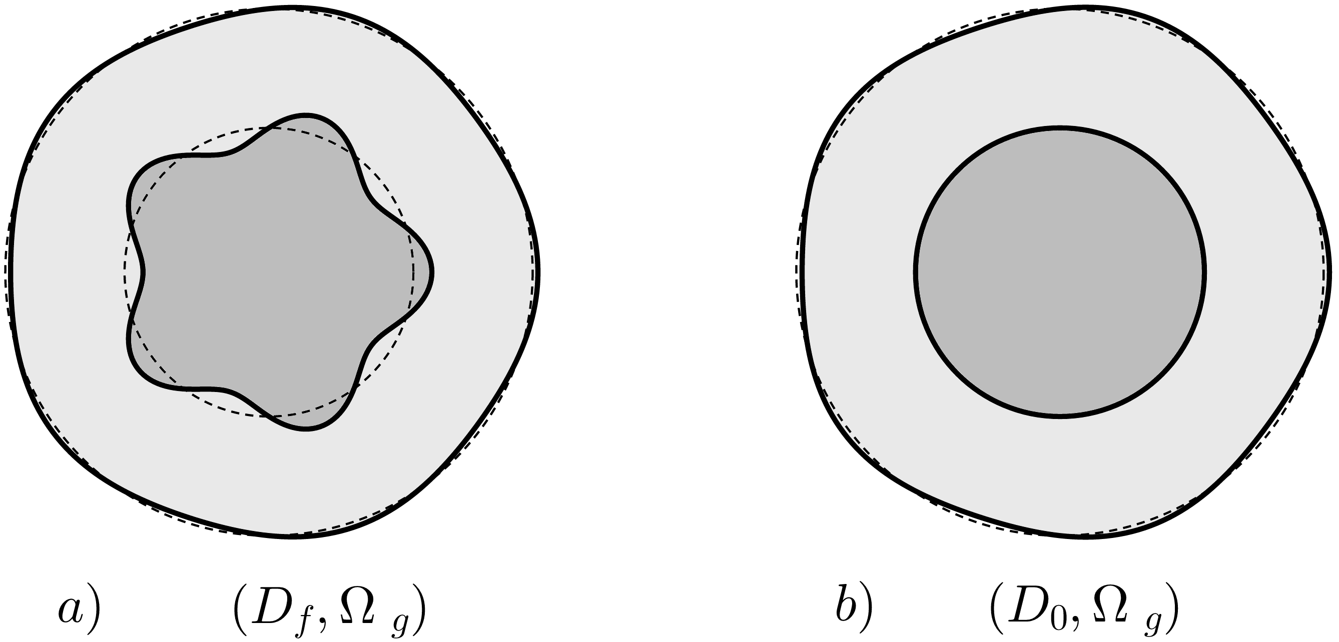
Figure 2: a) A nontrivial solution for $\sigma_{c}\notin\Sigma$, given by Theorem II. b) A symmetry breaking solution branching from the trivial solution $(D_{0},\Omega_{0})$ at the bifurcation point $\sigma_{c}=s_{k}$, given by Theorem III.

Theorem III.

Take an element $s_{k}\in\Sigma$ and consider the equation

$$\Psi(g,s)=\Phi(0,g,s)=0,$$

then $(0,s_{k})\in{\mathcal{G}}\times\mathbb{R}$ is a bifurcation point of the equation $\Psi(g,s)=0$. That is, there exists a function $\varepsilon\mapsto\lambda(\varepsilon)\in\mathbb{R}$ with $\lambda(0)=0$ such that overdetermined problem (1.2)–(1.4) admits a nontrivial solution of the form $(D_{0},\Omega_{g(\varepsilon)})$ for $\sigma_{c}=s_{k}+\lambda(\varepsilon)$ and $\varepsilon$ small. Moreover, there exists a spherical harmonic $Y_{k}$ of $k$-th degree, such that the symmetry breaking solution $(D_{0},\Omega_{g(\varepsilon)})$ satisfies

$$g(\varepsilon)=\varepsilon Y_{k}(\theta)+o(\varepsilon)\quad\text{as }\varepsilon\to 0.$$ (1.11)

In particular, there exist uncountably infinitely many nontrivial solutions of problem (1.2)–(1.4) where $D$ is a ball (spontaneous symmetry breaking solutions).

As the following theorem shows, the one phase case $D=\emptyset$ has a radically different behavior around trivial solutions.

Theorem IV.

Let $D=\emptyset$. Then, the trivial solutions of (1.2)–(1.4) are isolate solutions (in the sense of Definition 5.1).

This paper is organized as follows. In section 2, we study what happens for $d\geq\frac{N-1}{N}$ and give a proof of Theorem I by means of the Heintze–Karcher inequality and a symmetry theorem by Sakaguchi concerning a two phase overdetermined of Serrin type problem in the ball. In section 3, we prove Theorem II and construct nontrivial solutions to (1.2)–(1.4) by using the implicit function theorem for Banach spaces and shape derivatives. Section 4 is devoted to the study of spontaneous symmetry breaking solutions that arise when $\sigma_{c}$ is a critical value. Here we prove Theorem III by means of the Crandall–Rabinowitz theorem. In Section 5 we show that, in the one phase setting, balls are isolated solutions (Theorem IV). Section 6 is devoted to the comparison between the overdetermined problem presented in this paper and a similar two phase overdetermined problem of Serrin type. Finally, in the appendix, we prove a technical result concerning invariant subgroups of spherical harmonics that is crucial to the proof of Theorem III in general dimension.

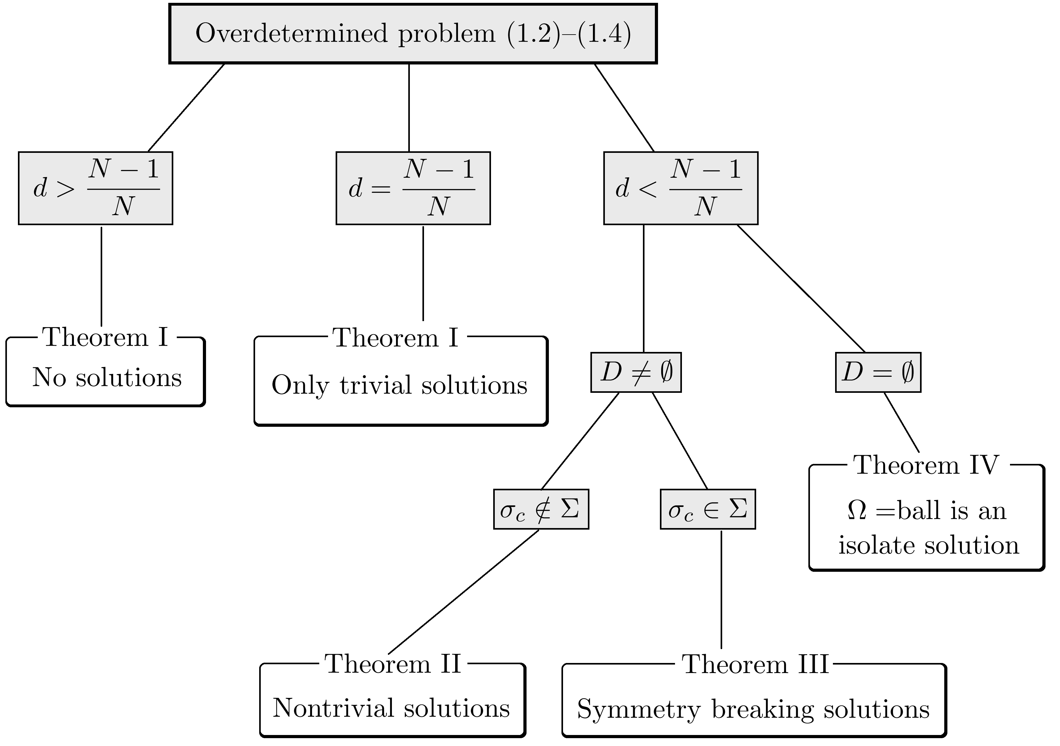
Figure 3: Organization of this paper

2 Only trivial solutions for $d=\frac{N-1}{N}$

The proof of Theorem I relies on the following two facts. The first is the so-called Heintze–Karcher inequality. This result was first proved for compact and embedded manifolds by Montiel and Ros in [MR] following the ideas of [HK]. It was then extended to general sets of finite perimeter in [San].

Theorem A (Heintze–Karcher inequality).

Let $\Omega$ be a bounded domain of class $\mathcal{C}^{2}$. Then the following inequality holds

$$\int_{\partial\Omega}1/H\geq\frac{N}{N-1}|\Omega|.$$

Moreover, equality is attained in the above if and only if $\Omega$ is a ball.

The second tool that we will need concerns the following two-phase overdetermined problem of Serrin-type:

$$-\mathop{\mathrm{div}}\left(\sigma\nabla u\right)=1\quad\text{in }\Omega,$$ (2.12)

$$u=0\quad\text{on }\partial\Omega,$$ (2.13)

$$\partial_{n}u=-c\quad\text{on }\partial\Omega,$$ (2.14)

where $c$ is some given positive constant. The following theorem is a special case of Theorem 5.1 of [Sak2].

Theorem B (Symmetry for two phase Serrin problem in the ball, [Sak2]).

Let $\Omega\subset{\mathbb{R}}^{N}$ be an open ball and let $\emptyset\neq D\subset\overline{D}\subset\Omega$ be an open set of class $\mathcal{C}^{2}$, with at most finitely many connected components, and such that $\Omega\setminus D$ is connected. Now, if $(D,\Omega)$ is a solution of the overdetermined problem (2.12)–(2.14), then $D$ must be a ball concentric with $\Omega$.

Proof of Theorem I.

Let $(D,\Omega)$ be a solution of problem (1.2)–(1.4) for some positive real number $d$. We recall that, since both $D$ and $\Omega$ are of class $\mathcal{C}^{2}$, the boundary value problem (1.2)–(1.3) admits the following equivalent formulation as a transmission problem ([AS, Theorem 1.1]):

$$\begin{cases}-\sigma_{c}\Delta u=1\quad\text{in }D,\\ -\Delta u=1\quad\text{in }\Omega\setminus\overline{D},\\ [u]=[\sigma\partial_{n}u]=0\quad\text{on }\partial D,\\ u=0\quad\text{on }\partial\Omega,\end{cases}$$ (2.15)

where brackets are used to denote the jump of a quantity along the interface $\partial D$.

By (2.15), with the aid of the divergence theorem, we get

$$|\Omega|=\int_{D}1+\int_{\Omega\setminus\overline{D}}1=-\sigma_{c}\int_{D}\Delta u-\int_{\Omega\setminus\overline{D}}\Delta u=-\int_{\partial D}[\sigma\partial_{n}u]-\int_{\partial\Omega}\partial_{n}u=-\int_{\partial\Omega}\partial_{n}u.$$

Now, the overdetermined condition (1.4) and Heintze–Karcher inequality yield

$$|\Omega|=-\int_{\partial\Omega}\partial_{n}u=d\int_{\partial\Omega}1/H\geq\frac{dN}{N-1}|\Omega|.$$

In particular, since $|\Omega|>0$, this implies that $d\leq\frac{N-1}{N}$, as claimed. Moreover, when $d=\frac{N-1}{N}$, then we deduce that $\Omega$ is a ball by the second part of Theorem A. In particular, $H$ is constant on $\partial\Omega$ and hence, the solution $u$ of problem (1.2)–(1.4) also solves the overdetermined condition (2.14) for some constant $c>0$. We conclude by Theorem B. ∎

Remark 2.1.

Notice that, since $\partial_{n}u<0$ on $\partial\Omega$ by Hopf’s lemma, if the pair $(D,\Omega)$ is a solution of (1.2)–(1.4), then $\Omega$ must be a strictly mean convex set (that is, $H>0$ on $\partial\Omega$).

3 Local existence of nontrivial solutions for $\sigma_{c}\notin\Sigma$

The proof of Theorem II will rely on the following version of the implicit function theorem for Banach spaces (see [AP, Theorem 2.3, page 38] for a proof).

Theorem C (Implicit function theorem).

Let $\Psi\in\mathcal{C}^{k}(\Lambda\times W,Y)$, $k\geq 1$, where $Y$ is a Banach space and $\Lambda$ (resp. $U$) is an open set of a Banach space $T$ (resp. $X$). Suppose that $\Psi(\lambda^{*},w^{*})=0$ and that the partial derivative $\partial_{w}\Psi(\lambda^{*},w^{*})$ is a bounded invertible linear transformation from $X$ to $Y$.

Then there exist neighborhoods $\Theta$ of $\lambda^{*}$ in $T$ and $W^{*}$ of $w^{*}$ in $X$, and a map $g\in\mathcal{C}^{k}(\Theta,X)$ such that the following hold:

1. $\Psi(\lambda,g(\lambda))=0$ for all $\lambda\in\Theta$,

2. If $\Psi(\lambda,u)=0$ for some $(\lambda,u)\in\Theta\times U^{*}$, then $u=g(\lambda)$,

3. $g^{\prime}(\lambda)=-\left(\partial_{u}\Psi(p)\right)^{-1}\circ\partial_{\lambda}\Psi(p)$, where $p=(\lambda,g(\lambda))$ and $\lambda\in\Theta$.

3.1 Preliminaries

Let $\mathcal{F}$ and ${\mathcal{G}}$ be the sets defined in (1.6) and let ${\mathcal{H}}$ be the following

$${\mathcal{H}}=\left\{h\in\mathcal{C}^{\alpha}(\partial\Omega_{0})\;\mathrel{\mathop{\mathchar 58\relax}}\;\int_{\partial\Omega_{0}}h=0\right\}.$$

The sets $\mathcal{F}$, ${\mathcal{G}}$ and ${\mathcal{H}}$ are Banach spaces, endowed with the natural norm of the corresponding Hölder class. We will apply the implicit function theorem to the following mapping.

$$\Phi\mathrel{\mathop{\mathchar 58\relax}} \mathcal{F}\times{\mathcal{G}}\times(0,\infty)\longrightarrow{\mathcal{H}}$$ (3.16)

$$(f,g,s)\longmapsto\Pi_{0}\left(\partial_{n_{g}n_{g}}^{2}u_{f,g}\right),$$

where $\Pi_{0}\mathrel{\mathop{\mathchar 58\relax}}\mathcal{C}^{\alpha}(\partial\Omega_{0})\to{\mathcal{H}}$ is the projection operator, defined by

$$\Pi_{0}(\varphi)=\varphi-\frac{1}{|\partial\Omega_{0}|}\int_{\partial\Omega_{0}}\varphi,$$

and $u_{f,g}$ is the solution of (1.2)–(1.3) with $\Omega=\Omega_{g}$ and $\sigma=s\mathcal{X}_{D_{f}}+\mathcal{X}_{\Omega_{g}\setminus D_{f}}$. Moreover, by a slight abuse of notation, $\partial_{n_{g}n_{g}}^{2}u_{f,g}$ denotes the function of value

$$n_{g}\big{(}x+g(x)n(x)\big{)}\cdot\left(D^{2}u_{f,g}\big{(}x+g(x)n(x)\big{)}\ n_{g}\big{(}x+g(x)n(x)\big{)}\right)\;\text{at any }x\in\partial\Omega_{0}.$$ (3.17)

Remark 3.1 (Zeros of $\Phi(\cdot,\cdot,\sigma_{c})$ correspond to solutions of (1.2)–(1.4)).

Notice that, by definition, $\Phi(f,g,\sigma_{c})=0$ if and only if the function defined in (3.17) takes the same value for all $x\in\partial\Omega_{0}$, that is, if and only if $\partial_{n_{g}n_{g}}^{2}u_{f,g}(\cdot)$ is constant on $\partial\Omega_{g}$. In other words, $\Phi(f,g,\sigma_{c})=0$ if and only if the pair $(D_{f},\Omega_{g})$ is a solution to the overdetermined problem (1.2)–(1.4). Indeed, applying the well-known decomposition formula for the Laplace operator

$$\Delta\varphi=\partial_{nn}^{2}\varphi+H\partial_{n}\varphi+\Delta_{\tau}\varphi\quad\text{on }\partial\omega\quad(\omega\in\mathcal{C}^{2},\ \varphi\in\mathcal{C}^{2}(\overline{\omega}))$$ (3.18)

to the function $u_{f,g}$ yields that the product $H\partial_{n}u_{f,g}$ is constant on $\partial\Omega_{g}$. Therefore, if $H$ never vanishes on $\partial\Omega_{g}$ (which holds true if $g$ is small enough, by continuity), then we recover the overdetermined condition (1.4).

In the rest of this section, we will fix $\sigma_{c}\notin\Sigma$ and apply Theorem C to the map $\Psi(\cdot,\cdot)\mathrel{\mathop{\mathchar 58\relax}}=\Phi(\cdot,\cdot,\sigma_{c})$.

3.2 Computing the derivative of $\Psi$

The differentiability of the map $(f,g)\mapsto\Phi(f,g,\sigma_{c})$ derives from that of the function $u_{f,g}$ and its spatial derivatives up to second order (indeed, notice that $n_{g}=-\nabla u_{f,g}/|\nabla u_{f,g}|$ on $\partial\Omega_{g}$, because $\partial\Omega_{g}$ is a level set of $u_{f,g}$ by construction). In turn, the Fréchet differentiability of both $u_{f,g}$ and its spatial derivatives can be proved in a standard way, by following the proof of [HP, Theorem 5.3.2, pages 206–207] with the help of the regularity theory for elliptic operators with piecewise constant coefficients. In particular, the Hölder continuity of the first and second derivatives of the function $u_{f,g}$ up to the interface $\partial D_{f}$, which is stated in [LU, Theorem 16.2, page 222], is obtained by flattening the interface with a diffeomorphism of class $\mathcal{C}^{2,\alpha}$ as in [LU, Chapter 4, Section 16, pages 205–223] or in [DEF, Appendix, pages 894–900] and by using the classical regularity theory for linear elliptic partial differential equations ([LU, Gi, ACM]).

Now, for fixed $g_{0}\in{\mathcal{G}}$ and small enough $\varepsilon>0$, consider the map

$$(-\varepsilon,\varepsilon)\ni t\mapsto u_{t}\mathrel{\mathop{\mathchar 58\relax}}=u_{0,tg_{0}}.$$ (3.19)

For any given point $x\in\Omega_{0}$, notice that $x\in\Omega_{tg_{0}}$ if $t>0$ is sufficiently small. Therefore it makes sense to consider the following limit:

$$\lim_{t\to 0}\frac{u_{t}(x)-u(x)}{t}.$$

When well defined, the quantity above will be referred to as the shape derivative of $u$ and will be denoted by $u^{\prime}(x)$. The following lemma gives a characterization of the shape derivative of $u$ and it will be crucial for the upcoming computations. For a proof, we refer the interested reader to [Ca1, Proposition 3.1] (see also [Ca2, Theorem 3.21]).

Lemma 3.2.

Let $g_{0}\in{\mathcal{G}}$ be fixed, and let the map $(-\varepsilon,\varepsilon)\ni t\mapsto u_{t}$ be as above. Then the shape derivative $u^{\prime}$ of $u$ is well defined at all points $x\in\Omega_{0}$. Moreover, $u^{\prime}$ can be characterized as the solution of the following boundary value problem:

$$\begin{cases}-\mathop{\mathrm{div}}(\sigma\nabla u^{\prime})=0\quad\text{in }\Omega_{0},\\ u^{\prime}=g_{0}/N\quad\text{on }\partial\Omega_{0}.\end{cases}$$ (3.20)

Theorem 3.3.

The map $\Phi(\cdot,\cdot,\sigma_{c})\mathrel{\mathop{\mathchar 58\relax}}\mathcal{F}\times{\mathcal{G}}\to{\mathcal{H}}$ is of class $\mathcal{C}^{\infty}$ in a neighborhood of $(0,0)$ and its partial Fréchet derivative with respect to the second variable defines a continuous linear mapping from ${\mathcal{G}}$ to ${\mathcal{H}}$ defined by the formula

$$\partial_{g}\Psi(0,0,\sigma_{c})[g_{0}]=\partial_{nn}^{2}u^{\prime}\quad\text{for }g_{0}\in{\mathcal{G}},$$ (3.21)

where $u^{\prime}$ is the solution to (3.20).

The proof of Theorem 3.3 will be given later, as some preliminary work is required. From now on, we fix an element $g_{0}\in{\mathcal{G}}$, set $f=0$ and, in order to simplify notations, write $\Omega_{t},u_{t},n_{t}$ in place of $\Omega_{tf},u_{tf,0},n_{tg}$. Moreover, for $x\in\Omega_{0}$, we set

$$b_{t}(x)=\nabla u_{t}(x+tg_{0}(x)n(x))\quad\text{and}\quad A_{t}(x)=D^{2}u_{t}(x+tg_{0}(x)n(x)).$$ (3.22)

Whenever confusion does not arise, we will omit the subscript $0$ and write $u$ for $u_{0}$, $n$ for $n_{0}$, $b$ and $A$ for $b_{0}$ and $A_{0}$ and so on. The following lemma contains all the ingredients needed for the proof of Theorem 3.3.

Lemma 3.4.

The functions $b_{t}$ and $A_{t}$ defined in (3.22) are differentiable with respect to the variable $t$ in a neighborhood of $t=0$. Moreover, the following hold true

$$b=-\frac{1}{N}n,\quad A=-\frac{1}{N}I,\quad\dot{b}\mathrel{\mathop{\mathchar 58\relax}}={\left.\kern-1.2pt\frac{d}{dt}\vphantom{|}\right|_{t=0}}b_{t}=\nabla u^{\prime}-\frac{g_{0}}{N}n,\quad\dot{A}\mathrel{\mathop{\mathchar 58\relax}}={\left.\kern-1.2pt\frac{d}{dt}\vphantom{|}\right|_{t=0}}A_{t}=D^{2}u^{\prime}.$$ (3.23)

Proof.

The first two identities are an immediate consequence of the explicit expression in (1.5). The differentiability of $b_{t}$ and $A_{t}$ with respect to $t$ ensues by standard results concerning shape derivatives (for instance, see [HP] or [DZ]). The remaining identities in (3.23) can be proved as follows.

$$\dot{b}(x)={\left.\kern-1.2pt\frac{d}{dt}\vphantom{|}\right|_{t=0}}\nabla u_{t}(x+tg_{0}(x)n(x))=\nabla u^{\prime}(x)+g_{0}(x)D^{2}u(x)n(x)=\nabla u^{\prime}(x)-\frac{g_{0}(x)}{N}n(x),$$

where the last equality ensues from (1.5). Analogously, for the last identity we get

$$\dot{A}(x)={\left.\kern-1.2pt\frac{d}{dt}\vphantom{|}\right|_{t=0}}D^{2}u_{t}(x+tg_{0}(x)n(x))=D^{2}u^{\prime}(x)+g_{0}(x)D^{3}u(x)n(x)=D^{2}u^{\prime}(x),$$

where, in the last equality, we used the fact that $D^{3}u=0$ because $u$ is quadratic in a neighborhood of $\partial\Omega_{0}$ (again, by (1.5)). ∎

Proof of Theorem 3.3.

Since $\Phi$ is Fréchet differentiable, we can compute $\partial_{g}\Phi(0,0,\sigma_{c})$ as a Gâteaux derivative:

$$\partial_{g}\Phi(0,0,\sigma_{c})[g_{0}]=\lim_{t\to 0^{+}}\frac{\Phi(0,tg_{0},\sigma_{c})-\Phi(0,0,\sigma_{c})}{t}\quad\text{for }g_{0}\in{\mathcal{G}}.$$ (3.24)

First of all, notice that, for fixed $g_{0}\in{\mathcal{G}}$, the map $\Phi(0,tg_{0},\sigma_{c})$ can be expressed by means of the auxiliary functions $b_{t}$ and $A_{t}$ defined in (3.22):

$$\Phi(0,tg_{0},\sigma_{c})=c_{t}-\frac{1}{|\partial\Omega_{t}|}\int_{\partial\Omega_{t}}c_{t},\qquad\text{where }c_{t}=\frac{b_{t}\cdot(A_{t}b_{t})}{|b_{t}|^{2}}.$$

Let us first focus on the derivative of $c_{t}$. By the quotient rule, we have

$${\left.\kern-1.2pt\frac{d}{dt}\vphantom{|}\right|_{t=0}}c_{t}={\left.\kern-1.2pt\frac{d}{dt}\vphantom{|}\right|_{t=0}}\left(\frac{b_{t}\cdot(A_{t}b_{t})}{|b_{t}|^{2}}\right)=\frac{|b|^{2}(2\dot{b}\cdot Ab+b\cdot\dot{A}b)-2b\cdot\dot{b}(b\cdot Ab)}{|b|^{4}}$$

Substituting the expressions for $b$, $A$, $\dot{b}$ and $\dot{A}$ from (3.23) into the expression above yields

$${\left.\kern-1.2pt\frac{d}{dt}\vphantom{|}\right|_{t=0}}c_{t}=-{2}{\left(\nabla u^{\prime}-\frac{g_{0}}{N}n\right)}\cdot n+\partial_{nn}^{2}u^{\prime}+{2}\left(\nabla u^{\prime}-\frac{g_{0}}{N}n\right)\cdot n=\partial_{nn}^{2}u^{\prime}.$$ (3.25)

Now, let us compute the derivative of the remaining term in (3.24) with (3.25) at hand. By employing the use of the well-known formula for the shape derivative of the perimeter (see [HP, Corollary 5.4.16 and underneath remarks, page 224])

$${\left.\kern-1.2pt\frac{d}{dt}\vphantom{|}\right|_{t=0}}|\partial\Omega_{t}|=\int_{\partial\Omega_{0}}Hg_{0},$$

we obtain

$${\left.\kern-1.2pt\frac{d}{dt}\vphantom{|}\right|_{t=0}}\left(\frac{1}{|\partial\Omega_{t}|}\int_{\partial\Omega_{t}}c_{t}\right)=\frac{|\partial\Omega_{0}|\int_{\partial\Omega_{0}}\partial_{nn}^{2}u^{\prime}-\int_{\partial\Omega_{0}}Hg_{0}\int_{\partial\Omega_{0}}\partial_{nn}^{2}u}{|\partial\Omega_{0}|^{2}}=\frac{1}{|\partial\Omega_{0}|}\int_{\partial\Omega_{0}}\partial_{nn}^{2}u^{\prime},$$ (3.26)

where in the last equality we used the fact that $H$ is constant on $\partial\Omega_{0}$ and that $g_{0}\in{\mathcal{G}}$ has vanishing average by hypothesis. The claim of the theorem follows if we manage to show that the integral of $\partial_{nn}^{2}u^{\prime}$ over $\partial\Omega_{0}$ vanishes. In order to show this, let us apply (3.18) to $u^{\prime}$. We get

$$\int_{\partial\Omega_{0}}\partial_{nn}^{2}u^{\prime}=-H\int_{\partial\Omega_{0}}\partial_{n}u^{\prime}+\int_{\partial\Omega_{0}}\Delta_{\tau}g_{0}=-H\int_{\partial\Omega_{0}}\partial_{n}u^{\prime}.$$ (3.27)

In a similar way to what we did in the proof of Theorem I, by the divergence theorem we conclude that

$$0=\sigma_{c}\int_{D_{0}}\Delta u^{\prime}+\int_{\Omega_{0}\setminus\overline{D_{0}}}\Delta u^{\prime}=\int_{\partial D_{0}}[\sigma\partial_{n}u^{\prime}]+\int_{\partial\Omega_{0}}\partial_{n}{u^{\prime}}=\int_{\partial\Omega_{0}}\partial_{n}u^{\prime}.$$ (3.28)

The claim follows by combining (3.25),(3.26), (3.27) and (3.28). ∎

3.3 Applying the implicit function theorem

In order to apply Theorem C, we will need the following explicit representation for $u^{\prime}$ as a spherical harmonic expansion. Let $\{Y_{k,i}\}_{k,i}$ ($k\in\{0,1,\dots\}$, $i\in\{1,2,\dots,d_{k}\}$) denote a maximal family of linearly independent solutions to the eigenvalue problem

$$-\Delta_{\tau}Y_{k,i}=\lambda_{k}Y_{k,i}\quad\textrm{ on }\SS^{N-1},$$

with $k$-th eigenvalue $\lambda_{k}=k(N+k-2)$ of multiplicity $d_{k}$ and normalized in such a way that $\mathinner{\!\left\lVert Y_{k,i}\right\rVert}_{L^{2}(\SS^{N-1})}=1$. Here $\Delta_{\tau}$ stands for the Laplace–Beltrami operator on the unit sphere $\SS^{N-1}$. Such functions, usually referred to as spherical harmonics in the literature, form a complete orthonormal system of $L^{2}(\SS^{N-1})$. Notice that the eigenspace corresponding to the eigenvalue $\lambda_{0}=0$ is the 1-dimensional space of constant functions on $\SS^{N-1}$. Moreover, notice that such constant function term does not appear in the expansion of a function of zero average on $\SS^{N-1}$. We refer to [Ca1, Proposition 3.2] for a proof of the following result.

Lemma 3.5.

Assume that, for some real coefficients $\alpha_{k,i}$, the following expansion holds true in $L^{2}(\SS^{N-1})$:

$$g_{0}(\theta)=\sum_{k=1}^{\infty}\sum_{i=1}^{d_{k}}\alpha_{k,i}Y_{k,i}(\theta).$$ (3.29)

Then, the function $u^{\prime}$, solution to (3.20), admits the following explicit expression for $\theta\in\mathbb{S}^{N-1}$ and $r\in[0,1]$:

$$u^{\prime}(r\theta)=\begin{cases}\displaystyle\sum_{k=1}^{\infty}\sum_{i=1}^{d_{k}}\alpha_{k,i}B_{k}r^{k}Y_{k,i}(\theta)\quad&\text{ for }r\in[0,R],\\ \displaystyle\sum_{k=1}^{\infty}\sum_{i=1}^{d_{k}}\alpha_{k,i}\left(C_{k}r^{2-N-k}+D_{k}r^{k}\right)Y_{k,i}(\theta)\quad&\text{ for }r\in(R,1],\end{cases}$$ (3.30)

where $R\in(0,1)$ and the coefficients $B_{k}$, $C_{k}$ and $D_{k}$ are defined as follows:

$$B_{k}=(N-2+2k)R^{2-N-2k}/F,\quad C_{k}=(1-\sigma_{c})k/F,\quad D_{k}=(N-2+k+k\sigma_{c})R^{2-N-2k}/F,$$

and the common denominator $F=N(N-2+k+k\sigma_{c})R^{2-N-2k}+kN(1-\sigma_{c})$.

When $D=\emptyset$, that is $R=0$ (or $\sigma_{c}=1$), then the above simplifies to

$$u^{\prime}(r\theta)=\sum_{k=1}^{\infty}\sum_{i=1}^{d_{k}}\frac{r^{k}}{N}\alpha_{k,i}Y_{k,i}(\theta).$$

Remark 3.6.

The quantity $F=N(N-2+k+k\sigma_{c})R^{2-N-2k}+kN(1-\sigma_{c})$ is strictly positive if $R\in(0,1)$ and $k\geq 1$. Indeed we have

$$F>N(N-2+k+k\sigma_{c})+kN(1-\sigma_{c})=N^{2}+2N(k-1)\geq N^{2}>0.$$

Now, with Theorem 3.3 and expansion (3.30) at hand, it is easy to check that the partial Fréchet derivative $\partial_{g}\Phi(0,0,\sigma_{c})$ yields the following map from ${\mathcal{G}}$ into ${\mathcal{H}}$ defined by:

$$\sum_{k=1}^{\infty}\sum_{i=1}^{d_{k}}\alpha_{k,i}Y_{k,i}\longmapsto\sum_{k=1}^{\infty}\sum_{i=1}^{d_{k}}\alpha_{k,i}\beta_{k}Y_{k,i},\quad\text{where }$$ (3.31)

$$\beta_{k}=\beta_{k}(\sigma_{c})=k\ \frac{(2-N-k)(1-N-k)(1-\sigma_{c})+(k-1)(N-2+k+k\sigma_{c})R^{2-N-2k}}{kN(1-\sigma_{c})+N(N-2+k+k\sigma_{c})R^{2-N-2k}}.$$

We are now ready to apply the implicit function theorem to the mapping $\Phi(\cdot,\cdot,\sigma_{c})$.

Proof of Theorem II.

Since the Fréchet differentiability of $\Phi$ has already been dealt with in Theorem 3.3, in order to apply Theorem C of page C to $\Phi(\cdot,\cdot,\sigma_{c})$, we just need to ensure that the mapping defined by (3.21) (or, equivalently, (3.31)) is a bounded linear transformation from ${\mathcal{G}}$ to ${\mathcal{H}}$. Linearity and boundedness ensue from the properties of the boundary value problem (3.20). We are left to show that $\partial_{g}\Phi(0,0,\sigma_{c})\mathrel{\mathop{\mathchar 58\relax}}{\mathcal{G}}\to{\mathcal{H}}$ is a bijection. Injectivity is immediate, once one realizes that, for $k\geq 1$, the coefficient $\beta_{k}$ in (3.31) vanishes if and only if $\sigma_{c}=s_{k}$ (in retrospective, we can say that $s_{k}$ was defined in order to have this property). This implies that the map $\partial_{g}\Phi(0,0,\sigma_{c})$ is injective as long as $\sigma_{c}\notin\Sigma$. Let us now show surjectivity. Take an arbitrary function $h_{0}\in{\mathcal{H}}$. Since, in particular, $h_{0}$ is continuous on $\partial\Omega_{0}$, it admits a spherical harmonic expansion, say

$$h_{0}=\sum_{k=1}^{\infty}\sum_{i=0}^{d_{k}}\gamma_{k,i}Y_{k,i}.$$

Set now

$$g_{0}=\sum_{k=1}^{\infty}\sum_{i=0}^{d_{k}}\frac{\gamma_{k,i}}{\beta_{k}}Y_{k,i}.$$ (3.32)

First of all, notice that, since the sequence $1/\beta_{k}$ is bounded, the function $g_{0}$ above is a well defined element of $L^{2}(\partial\Omega_{0})$. Moreover, the integral of $g_{0}$ over $\partial\Omega_{0}$ vanishes because the summation in (3.32) starts from $k=1$. Finally, if we let $\mathcal{L}$ denote the continuous extension to $L^{2}(\partial\Omega_{0})\to L^{2}(\partial\Omega_{0})$ of the map defined by (3.31), it is clear that $g_{0}=\mathcal{L}^{-1}(h_{0})$ by construction. Therefore, in order to prove the surjectivity of the original map $\partial_{g}\Phi(0,0,\sigma_{c})$, we just need to show that the function $g_{0}$, defined in (3.32), is of class $\mathcal{C}^{2,\alpha}$ whenever $h_{0}\in\mathcal{C}^{\alpha}$. To this end, we will employ the use of various facts from classical regularity theory. First of all, we recall that functions in the Sobolev space $H^{s}(\partial\Omega_{0})$ can be characterized by the decay of the coefficients of their spherical harmonic expansion as follows:

$$\sum_{k=1}^{\infty}\sum_{i=0}^{d_{k}}(1+k^{2})^{s}\alpha_{k,i}^{2}<\infty\iff\sum_{k=1}^{\infty}\sum_{i=0}^{d_{k}}\alpha_{k,i}^{2}Y_{k,i}\in H^{s}(\partial\Omega_{0}).$$

Since $h_{0}\in\mathcal{C}^{\alpha}(\partial\Omega_{0})\subset L^{2}(\partial\Omega_{0})$, the asymptotic behavior of the coefficients $\beta_{k}$ given in (3.31) yields that $g_{0}\in H^{2}(\partial\Omega_{0})$. Now, if we define $u^{\prime}$ to be the solution to (3.20) whose $g_{0}$ in the boundary condition is given by (3.32), then we also obtain that ${\left.\kern-1.2pt\partial_{nn}^{2}u^{\prime}\vphantom{|}\right|_{\partial\Omega_{0}}}=h_{0}$ and ${\left.\kern-1.2pt\partial_{n}u^{\prime}\vphantom{|}\right|_{\partial\Omega_{0}}}\in H^{1}(\partial\Omega_{0})$. The next step employs the use of the decomposition formula (3.18), which still holds true by a density argument. We get

$$\partial_{nn}^{2}u^{\prime}+H\partial_{n}u^{\prime}+1/N\ \Delta_{\tau}g_{0}=0\quad\text{on }\partial\Omega_{0}.$$

That is,

$$h_{0}+(N-1)\partial_{n}u^{\prime}+1/N\ \Delta_{\tau}g_{0}=0\quad\text{on }\partial\Omega_{0}.$$ (3.33)

The identity above implies that, in particular, $\Delta_{\tau}g_{0}$ belongs to $L^{p}(\partial\Omega_{0})$ for $p=\frac{2N}{N-1}$. Therefore, by the standard $L^{p}$ theory for the Laplace equation on manifolds, we get that $g_{0}\in W^{2,p}(\partial\Omega_{0})$. Then, by the trace theorem for general Sobolev spaces, $u^{\prime}$ is of class $W^{2+\frac{1}{p},p}$ in a interior tubular neighborhood of $\partial\Omega_{0}$, and hence ${\left.\kern-1.2pt\partial_{n}u^{\prime}\vphantom{|}\right|_{\partial\Omega_{0}}}\in W^{1,p}(\partial\Omega_{0})$. This fact, together with (3.33), implies that ${\left.\kern-1.2pt\partial_{n}u^{\prime}\vphantom{|}\right|_{\partial\Omega_{0}}}$ belongs to an $L^{q}$ space with a higher integration exponent $q$. Iterating this process one gets that ${\left.\kern-1.2pt\partial_{n}u^{\prime}\vphantom{|}\right|_{\partial\Omega_{0}}}\in W^{1,p}(\partial\Omega_{0})$ for all $p>1$. Thus, by Morrey’s inequality, $\partial_{n}u^{\prime}$ also belongs to $\mathcal{C}^{\alpha}(\partial\Omega_{0})$. Going back to the identity (3.33), this implies that also $\Delta_{\tau}g_{0}\in\mathcal{C}^{\alpha}(\partial\Omega_{0})$ and thus, by the Schauder theory for the Laplace operator on manifolds, we finally obtain that $g_{0}\in\mathcal{C}^{2,\alpha}(\partial\Omega_{0})$, as claimed. This concludes the proof of the invertibility of the map $\partial_{g}\Phi(0,0,\sigma_{c})\mathrel{\mathop{\mathchar 58\relax}}{\mathcal{G}}\to{\mathcal{H}}$ and thus that of Theorem II. ∎

4 Symmetry breaking bifurcation at $\sigma_{c}\in\Sigma$

In this section we will show the local behavior of nontrivial solutions to (1.2)–(1.4) near the trivial solution $(D_{0},\Omega_{0})$ when $\sigma_{c}\in\Sigma$. To this end, we will employ the use of the following version of the Crandall–Rabinowitz theorem (that is equivalent to the one stated in [CR]). Although, nowadays, the Crandall–Rabinowitz theorem can be regarded as a staple of bifurcation theory for partial differential equations, to the best of my knowledge its applications to overdetermined problems are not so well-known (see [Oka, FR, EM, KS, CY2] for some literature).

Theorem D (Crandall–Rabinowitz theorem [CR]).

Let $X$, $Y$ be real Banach spaces and let $U\subset X$ and $\Lambda\subset\mathbb{R}$ be open sets, such that $0\in U$. Let $\Psi\in\mathcal{C}^{p}(U\times\Lambda;Y)$ ($p\geq 3$) and assume that there exist $\lambda_{0}\in\Lambda$ and $x_{0}\in\mathcal{X}$ such that

1. $\Psi(0,\lambda)=0$ for all $\lambda\in\Lambda$;

2. ${\rm Ker}\ \partial_{x}\Psi(0,\lambda_{0})$ is a 1-dimensional subspace of $X$ spanned by $x_{0}$;

3. ${\rm Im}\ \partial_{x}\Psi(0,\lambda_{0})$ is a closed co-dimension 1 subspace of $Y$;

4. $\partial_{\lambda}\partial_{x}\Psi(0,\lambda_{0})[x_{0}]\notin{\rm Im}\ \partial_{x}\Psi(0,\lambda_{0})$.

Then $(0,\lambda_{0})$ is a bifurcation point of the equation $\Psi(x,\lambda)=0$ in the following sense. In a neighborhood of $(0,\lambda_{0})\in\mathcal{X}\times\Lambda$, the set of solutions of $\Psi(x,\lambda)=0$ consists of two $\mathcal{C}^{p-2}$-smooth curves $\Gamma_{1}$ and $\Gamma_{2}$ which intersect only at the point $(0,\lambda_{0})$. $\Gamma_{1}$ is the curve $\{(0,\lambda)\,\mathrel{\mathop{\mathchar 58\relax}}\,\lambda\in\Lambda\}$ and $\Gamma_{2}$ can be parametrized as follows, for small $\varepsilon>0$:

$$(-\varepsilon,\varepsilon)\ni t\mapsto\left(x(t),\lambda(t)\right)\in{\mathcal{U}}\times\Lambda,\text{ such that }\left(x(0),\lambda(0)\right)=(0,\lambda_{0}),\quad x^{\prime}(0)=x_{0}.$$

In what follows, we will try to apply Theorem D to study the local behavior of the map (which is different from the one that was used in the previous section)

$$\Psi(g,s)\mathrel{\mathop{\mathchar 58\relax}}=\Phi(0,g,s),\quad(g\in{\mathcal{G}},s>0),$$ (4.34)

around the bifurcation points $\lambda_{0}=s_{k}$. Unfortunately, we cannot directly apply Theorem  D in this setting because ${\rm Ker}\ \partial_{g}\Psi(0,0,s_{k})$ is not a $1$-dimensional vector space. In order to circumvent this problem, we will consider the restriction of $\Phi(0,\cdot,s_{k})$ to some particular invariant subspace of ${\mathcal{G}}$.

Here we recall the definition of invariant subspace. Let $G$ be a subgroup of the orthogonal group $O(N)$. We will say that a set $\omega\subset{\mathbb{R}}^{N}$ is $G$-invariant if $\gamma(\omega)=\omega$ for all $\gamma\in G$. Moreover, a real-valued function defined on a $G$-invariant domain $\omega$ is said to be $G$-invariant if

$$\varphi=\varphi\circ\gamma\quad\text{for all }\gamma\in G.$$

Suppose that $\sigma_{c}=s_{k}\in\Sigma$ for some $k$, and let $\mathcal{Y}_{k}$ denote the $k$-th eigenspace of $-\Delta_{\tau}$, that is, the subspace of $\mathcal{C}^{2,\alpha}(\partial\Omega_{0})$ spanned by $\{Y_{k,1},\dots,Y_{k,d_{k}}\}$. Moreover, let $G^{\ast}$ be a subgroup of $O(N)$ such that the invariant subspace

$$\mathcal{Y}_{k}^{\ast}=\left\{Y_{k}\in\mathcal{Y}_{k}\;\mathrel{\mathop{\mathchar 58\relax}}\;Y_{k}\text{ is $G^{\ast}$-invariant}\right\}\text{ is $1$-dimensional}$$ (4.35)

(see the Appendix, for a proof that $G^{\ast}={\rm Id}\times O(N-1)$ satisfies (4.35) for all $k\in\mathbb{N}$). Let us now define the following two invariant spaces:

$${\mathcal{G}}^{\ast}=\left\{g\in{\mathcal{G}}\;\mathrel{\mathop{\mathchar 58\relax}}\;g\text{ is $G^{\ast}$-invariant}\right\},\quad{\mathcal{H}}^{\ast}=\left\{h\in{\mathcal{H}}\;\mathrel{\mathop{\mathchar 58\relax}}\;h\text{ is $G^{\ast}$-invariant}\right\},$$

and let $\Phi^{\ast}(0,\cdot,\cdot)$ denote the restriction of $\Phi(0,\cdot,\cdot)$ to ${\mathcal{G}}^{\ast}\times(0,\infty)$. We claim that such a $\Phi^{\ast}(0,\cdot,\cdot)$ defines a mapping ${\mathcal{G}}^{\ast}\times(0,\infty)\to{\mathcal{H}}^{\ast}$. Indeed, for all $g\in{\mathcal{G}}^{\ast}$, we have that $(D_{0},\Omega_{g})$ is a pair of $G^{\ast}$-invariant domains. As a consequence, by the unique solvability of the boundary value problem (1.2)–(1.3), the function $u_{0,g}$ is $G^{\ast}$-invariant as well and, therefore, so is $\Phi(0,g,\sigma_{c})$, as claimed.

Proof of Theorem III.

Let $\sigma_{c}=s_{k}\in\Sigma$ and let $Y_{k}$ be an element in ${\mathcal{G}}^{\ast}$ that spans the 1- dimensional subspace $\mathcal{Y}_{k}^{\ast}$ defined in (4.35). In order to prove Theorem III we will just need to check conditions $(i)$–$(iv)$ of Theorem D with respect to the map $\Phi^{\ast}(0,\cdot,\cdot)\mathrel{\mathop{\mathchar 58\relax}}{\mathcal{G}}^{\ast}\times(0,\infty)\to{\mathcal{H}}^{\ast}$ at the bifurcation point $(0,s_{k})\in{\mathcal{G}}^{\ast}\times(0,\infty)$. Condition $(i)$ is clearly true, as it is equivalent to saying that the trivial solution $(D_{0},\Omega_{0})$ is a solution of the overdetermined problem (1.2)–(1.4) for all values of $\sigma_{c}>0$. Conditions $(ii)$ and $(iii)$ are also true because, by construction, the kernel ${\rm Ker}\ \partial_{g}\Phi^{\ast}(0,0,s_{k})=\mathcal{Y}_{k}^{\ast}$ is a 1-dimensional subspace of ${\mathcal{H}}^{\ast}$ spanned by $Y_{k}$, and, similarly, the image ${\rm Im}\ \partial_{g}\Phi^{\ast}(0,0,s_{k})={\mathcal{H}}^{\ast}/\mathcal{Y}_{k}^{\ast}$ is a closed subspace of ${\mathcal{H}}^{\ast}$ of codimension $1$. In what follows we will show that condition $(iv)$ also holds true. By (3.31),

$$\partial_{g}\Phi^{\ast}(0,0,s)[Y_{k}]=\beta_{k}(s)Y_{k}\quad\text{for }s>0,$$

which in turn implies

$$\partial_{s}\partial_{g}\Phi^{\ast}(0,0,s_{k})[Y_{k}]=\big{(}\partial_{s}\beta_{k}(s_{k})\big{)}Y_{k}.$$

In other words, in order for $(iv)$ to hold true, we need to show that the derivative $\partial_{s}\beta_{k}(s_{k})$ does not vanish. A direct computation of $\partial_{s}\beta_{k}(s_{k})$ is possible by recalling the definition of $\beta_{k}(s)$ in (3.31) and the fact that $\beta_{k}(s_{k})=0$ by the defining property of $s_{k}$. We obtain

$$\partial_{s}\beta_{k}(s_{k})=k\frac{-(k+N-2)(k+N-1)+k(k-1)R^{2-N-2k}}{kN(1-\sigma_{c})+N(N-2+k+k\sigma_{c})R^{2-N-2k}}.$$

By combining (1.9) and Remark 3.6 we get that $\partial_{s}\beta_{k}(s_{k})<0$ and, in particular, the function $\partial_{s}\partial_{g}\Phi^{\ast}(0,0,s_{k})[Y_{k}]$ does not belong to the image ${\rm Im}\ \partial_{g}\Phi^{\ast}(0,0,s_{k})$ as claimed. This concludes the proof of Theorem III. ∎

Remark 4.1.

We claim that all nontrivial solutions $(D_{0},\Omega_{g(\varepsilon)})$ given by Theorem III share the same symmetries of the element $x_{0}\in X^{*}$, defined such that ${\rm Ker}\,\partial_{x}\Psi^{*}(0,0)={\rm span}\{Y_{k}\}$. To this end, take a symmetry group $G\subset O(N)$ such that the function $Y_{k}$ is $G$-invariant. Now, consider the further restriction $\Psi^{**}$ of $\Psi^{*}$ to the subspace $X^{**}$ of all $G$-invariant functions in $X^{*}$. Notice that, since $Y_{k}$ is $G$-invariant by hypothesis, we have ${\rm Ker}\,\partial_{g}\Psi^{*}(0,0)={\rm Ker}\,\partial_{g}\Psi^{**}(0,0)={\rm span}\{Y_{k}\}$. Another application of the Crandall–Rabinowitz theorem to $\Psi^{**}$ yields that $g(\varepsilon)$ is also $G$-invariant. The claim follows by the arbitrariness of $G$.

5 More about the one phase case ($D=\emptyset$)

Let $\Omega_{0}$ denote the unit ball centered at the origin and let $\Omega_{g}$ be the perturbation of $\Omega_{0}$ by a function $g\in{\mathcal{G}}$ as defined in (1.7). We know that, when $D=\emptyset$, $\Omega_{0}$ is a solution of overdetermined problem (1.2)–(1.4) for $d=\frac{N-1}{N}$. In what follows, we will show that, unlike the two phase case $D\neq\emptyset$, trivial solutions are isolate solutions for (1.2)–(1.4) when $D$ is empty.

Definition 5.1 (Isolate solution).

We say that the trivial solution $\Omega_{0}$ is an isolate solution of (1.2)–(1.4) for $D=\emptyset$ if the following holds.

There exists some $\eta>0$ such that, for all elements $g_{0}\in{\mathcal{G}}$ with $\mathinner{\!\left\lVert g_{0}\right\rVert}_{\mathcal{C}^{2,\alpha}}<\eta$, the set $\Omega_{g_{0}}$ is a solution of (1.2)–(1.4) for some $d=d(g_{0})$ if and only if

$$\Omega_{g_{0}}=x_{0}+\Omega_{0}\quad\text{for some }x_{0}=x_{0}(g_{0})\in{\mathbb{R}}^{N}.$$

In other words, $\Omega_{0}$ is said to be a trivial solutions, if the only solutions of (1.2)–(1.4) in a neighborhood of $\Omega_{0}$ are precisely translations of $\Omega_{0}$.

In order to prove Theorem IV, we will make use of the following construction. Let $\mathcal{Y}_{1}$ denote the eigenspace of spherical harmonics corresponding to the first nonzero eigenvalue $\lambda_{1}=N-1$. $\mathcal{Y}_{1}$ is an $N$-dimensional space of analytic functions on the unit sphere $\partial\Omega_{0}$. Without loss of generality, we can write $\mathcal{Y}_{1}={\rm span}\left\{Y_{1,1},\dots,Y_{1,N}\right\}$, where $Y_{1,i}$ ($i=1,\dots,N$) are the functions defined by

$$Y_{1,i}(x)=\sqrt{\frac{N}{|\partial\Omega_{0}|}}\ x_{i},\quad\text{for }x=(x_{1},\dots,x_{N})\in\partial\Omega_{0}.$$ (5.36)

Moreover, let $\Pi_{1}\mathrel{\mathop{\mathchar 58\relax}}\mathcal{C}^{\alpha}(\partial\Omega_{0})\to\mathcal{Y}_{1}$ denote the projection operator onto the eigenspace $\mathcal{Y}_{1}$ and set $Q={\rm Id}-\Pi_{1}$. Consider now the following map:

$$\Psi\mathrel{\mathop{\mathchar 58\relax}}\;{\mathbb{R}}^{N}\times{\mathcal{G}} \longrightarrow{\mathbb{R}}^{N}\times({\mathcal{H}}/\mathcal{Y}_{1})$$

$$(y,g) \longmapsto\left({\rm Bar}\ \Omega_{g}-y,Q\Phi(g)\right),$$

where ${\rm Bar}\ A$ denotes the barycenter of the set $A$, that is, the point $\int_{A}x$, and by a slight abuse of notation, $\Phi(g)$ denotes the one-phase version of (3.16) (in other words, $\Phi(g)\mathrel{\mathop{\mathchar 58\relax}}=\Phi(0,g,1)$). The following lemma plays a key role in the proof of Theorem IV.

Lemma 5.2.

There exists a small positive real number $\varepsilon>0$ and a unique map $g\mathrel{\mathop{\mathchar 58\relax}}B_{\varepsilon}(0)\to{\mathcal{G}}$ such that the set of solutions of the equation $\Psi(y,g)=0$ around $(0,0)\in{\mathbb{R}}^{N}\times{\mathcal{G}}$ can be locally expressed as

$$\left\{(y,g)\in B_{\varepsilon}(0)\times{\mathcal{G}}\;\mathrel{\mathop{\mathchar 58\relax}}\;\Psi(y,g)=0\right\}=\left\{\left(y,g(y)\right)\;\mathrel{\mathop{\mathchar 58\relax}}\;y\in B_{\varepsilon}(0)\right\}.$$

Proof.

We will apply the implicit function theorem to the map $\Psi$ above. Indeed, $\Psi$ is a well-defined $\mathcal{C}^{1}$-mapping in a neighborhood of $(0,0)\in{\mathbb{R}}^{N}\times{\mathcal{G}}$ because both the barycenter function ${\rm Bar}(\cdot)$ and $\Phi(\cdot)$ are. Moreover, by construction, we have $\Psi(0,0)=(0,0)$.

In what follows, we will give the explicit formula for the Fréchet derivative $\partial_{g}\Psi(0,0)$. First of all, we recall the explicit formula for the Fréchet derivative of the barycenter function:

$${\left.\kern-1.2pt\left(\partial_{g}{\rm Bar}\ \Omega_{g}\right)\vphantom{|}\right|_{g=0}}[g_{0}]=\int_{\partial\Omega_{0}}g_{0}\ n\quad\text{for }g_{0}\in{\mathcal{G}}.$$ (5.37)

The expression in (5.37) can be obtained by applying the Hadamard formula to the real-valued functions $g\mapsto\int_{\Omega_{g}}x_{i}$ for $i=1,\dots,N$ (see, for instance, the second example in [HP, Subsection 5.9.3]). Now, combining the formula for the shape derivative of the barycenter (5.37) and Theorem 3.3 yields

$$\partial_{g}\Psi(0,0)[g_{0}]=\left(\int_{\partial\Omega_{0}}g_{0}\ n,\ Q\left(\partial_{nn}^{2}{\left.\kern-1.2ptu^{\prime}\vphantom{|}\right|_{\partial\Omega_{0}}}\right)\right),$$

where $u^{\prime}$ is the unique solution of (3.20) with $D=\emptyset$. Now, if we expand $g_{0}$ as in (3.29), then by Lemma 3.5 and (5.36) we get

$$\partial_{g}\Psi(0,0)\left[\sum_{k=1}^{\infty}\sum_{i=1}^{d_{k}}\alpha_{k,i}Y_{k,i}\right]=\left(\sqrt{\frac{\partial\Omega_{0}}{N}}\begin{pmatrix}\alpha_{1,1}\\ \vdots\\ \alpha_{1,N}\end{pmatrix},\ \sum_{k=2}^{\infty}\sum_{i=1}^{d_{k}}\frac{k(k-1)}{N}\alpha_{k,i}Y_{k,i}\right).$$

Now, by reasoning along the same lines as in the proof of Theorem II in section 3, we conclude that there exists a unique map $y\mapsto g(y)\in{\mathcal{G}}$ such that $\Psi(y,g(y))=0$ for $|y|$ sufficiently small. ∎

We are now ready to give a proof of Theorem IV.

Proof of Theorem IV.

First of all, notice that, if $\Omega_{g}$ solves overdetermined problem (1.2)–(1.4), then $\Psi({\rm Bar}\ \Omega_{g},g)=0$ (notice also that the converse is not necessarily true in general). In particular, for $|y|$ small, let $\widetilde{g}(y)$ denote the unique element in ${\mathcal{G}}$ such that

$$\Omega_{\widetilde{g}(y)}=y+\Omega_{0}.$$

We have that $\Psi(y,\widetilde{g}(y))=0$ and thus, by Lemma 5.2 there exists some $\varepsilon>0$ such that

$$g(y)=\widetilde{g}(y)\quad(\text{if }|y|<\varepsilon.$$ (5.38)

Let now $g_{0}$ be an element of ${\mathcal{G}}$ such that the set $\Omega_{g_{0}}$ solves (1.2)–(1.4), and put $x_{0}={\rm Bar}\ \Omega_{g_{0}}$. We claim that $\Omega_{g_{0}}=x_{0}+\Omega_{0}$ if $g_{0}$ is small enough. Indeed, notice that, by construction, $\Psi(x_{0},g_{0})=0$. Now, suppose that the function $g_{0}$ is sufficiently small, so that $|x_{0}|<\varepsilon$. Then, by Lemma 5.2, we obtain $g_{0}=g(x_{0})$. In particular, (5.38) yields that $g(x_{0})=\widetilde{g}(x_{0})$. Combining all these and then using the definition of $\widetilde{g}(\cdot)$, we get

$$\Omega_{g_{0}}=\Omega_{g(x_{0})}=\Omega_{\widetilde{g}(x_{0})}=x_{0}+\Omega_{0}.$$

Since the choice of $g_{0}\in{\mathcal{G}}$ was arbitrary, we conclude that $\Omega_{0}$ is an isolate solution as claimed. ∎

Remark 5.3.

We still do not know whether the only solutions of (1.2)–(1.4) are trivial when $D=\emptyset$. Indeed, Theorem IV (as it is stated) leaves open the possibility of solutions of the form $\Omega_{g}$ that suddenly appear for $\mathinner{\!\left\lVert g\right\rVert}_{\mathcal{C}^{2,\alpha}}$ large or even that of solutions with a more intricate topology corresponding to some nontrivial value $d<\frac{N-1}{N}$.

6 Comparison with the two phase Serrin overdetermined problem

In this section, we will analyze the main similarities and differences between the two phase overdetermined problems (1.2)–(1.4) and (2.12)–(2.14). The latter was first studied by Serrin in the ’70s in the case $D=\emptyset$ employing the moving planes method.

Theorem 6.1 ([Se]).

Let $D=\emptyset$. Then the overdetermined problem (2.12)–(2.14) admits a solution if and only if $\Omega$ is a ball.

Remark 6.2.

Notice that Theorem 6.1 is a global theorem, while Theorem IV is only local. One might wonder whether it is possible to extend Serrin’s proof to the overdetermined problem (1.2)–(1.4). The main difficulty lies in the following observation. The overdetermined condition (1.4) translates to an overdetermination on the second normal derivative and therefore, one cannot rely on the maximum principle (thus, the moving plane method) in any obvious way.

A crucial difference between the two overdetermined problems lies in the degrees of freedom given by the constants $d$ and $c$. Indeed, if $(D,\Omega)$ solves the two phase overdetermined problem of Serrin type (2.12)–(2.14), then by integration by parts we get $c=|\Omega|/|\partial\Omega|$. That is, the constant $c$, although independent of the core $D$, is not scaling invariant, and hence different trivial solutions might take different values of $c$. On the other hand, the constant $d$ in (1.4) is dimensionless. As a consequence, all trivial solutions of (1.2)–(1.4) share the same $d=\frac{N-1}{N}$ (and the converse is also true by Theorem I).

Remark 6.3.

The overdetermined condition of Serrin type (2.14) arises naturally in the context of shape optimization. Indeed, let $D$ and $\sigma_{c}$ be given and consider the following shape functional:

$$E(\Omega)=\int_{\Omega}\sigma_{c}|\nabla u|^{2},$$

where $u$ is the unique solution to (2.12)–(2.13). Indeed, if $\Omega$ is a critical shape of the functional $E(\cdot)$ among all domains of a given volume, then $u$ must automatically satisfy condition (2.14) (this is a consequence of the computations done in [Ca1]). To the best of my knowledge, it is still not known whether the overdetermined condition (1.4) also arises as an optimality condition for some sensible shape functional.

It is interesting to note that, the two phase overdetermined problems (1.2)–(1.4) and (2.12)–(2.14) show a nearly identical local behavior. Indeed, let $(D_{0},\Omega_{0})=(B_{R},B_{1})$ be a trivial solution and let $\mathcal{F}$, ${\mathcal{G}}$ denote the function spaces defined in (1.6). We know that there exists a finite set of critical values $\widetilde{\Sigma}$ such that the following two theorems hold true (compare the following with Theorem II and III respectively).

Theorem 6.4 ([CY1]).

Let $\sigma_{c}\notin\widetilde{\Sigma}$. Then, there exists a threshold $\varepsilon>0$ such that, for all $f\in\mathcal{F}$ satisfying $\mathinner{\!\left\lVert f\right\rVert}_{\mathcal{C}^{2,\alpha}}<\varepsilon$ there exists a function $g=g(f,\sigma_{c})\in{\mathcal{G}}$ such that the pair $(D_{f},\Omega_{g})$ is a solution to problem (2.12)–(2.14) for $c={|\Omega_{g}|}/{|\partial\Omega_{g}|}$. Moreover, this solution is unique in a small enough neighborhood of $(0,0)\in\mathcal{F}\times{\mathcal{G}}$. In particular, there exist infinitely many nontrivial solutions of problem (1.2)–(1.4).

Theorem 6.5 ([CY2]).

Take an element $s_{k}\in\widetilde{\Sigma}$ and set $D=D_{0}$. Then $(g,\sigma_{c})=(0,s_{k})\in{\mathcal{G}}\times\mathbb{R}$ is a bifurcation point for the overdetermined problem (2.12)–(2.14) in the following sense. There exists a function $\varepsilon\mapsto\lambda(\varepsilon)\in\mathbb{R}$ with $\lambda(0)=0$ such that overdetermined problem (2.12)–(2.14) admits a nontrivial solution of the form $(D_{0},\Omega_{g(\varepsilon)})$ for $\sigma_{c}=s_{k}+\lambda(\varepsilon)$ and $\varepsilon$ small. Moreover, there exists a spherical harmonic $Y_{k}$ of $k$-th degree, such that the symmetry breaking solution $(D_{0},\Omega_{g(\varepsilon)})$ satisfies

$$g(\varepsilon)=\varepsilon Y_{k}(\theta)+o(\varepsilon)\quad\text{as }\varepsilon\to 0.$$ (6.39)

In particular, there exist uncountably infinitely many nontrivial solutions of problem (2.12)–(2.14) where $D$ is a ball (spontaneous symmetry breaking solutions).

Finally, we show that, despite showing a very similar local behavior, the overdetermined problems (1.2)–(1.4) and (2.12)–(2.14) always give rise to different families of nontrivial solutions. Indeed, as the following result shows, the two overdetermined problems above are “independent” (in the sense that the only solutions that the two overdetermined problems share are the trivial ones).

Proposition 6.6.

Assume that the pair $(D,\Omega)$ satisfies the hypotheses stated in the introduction and solves both overdetermined problems (1.2)–(1.4) and (2.12)–(2.14) simultaneously for some constants $d$ and $c$. Then $\Omega$ is a ball and $D$ is either empty or a ball concentric with $\Omega$. Moreover, $d=\frac{N-1}{N}$ and $c=-\frac{|\partial\Omega|}{|\Omega|}$.

Proof.

By construction, the unique solution $u$ of the boundary value problem (1.2)–(1.3) solves both overdetermined conditions (1.4) and (2.14). In particular, $H$ is constant on $\partial\Omega$. Aleksandrov’s Soap Bubble Theorem (see [Al]) implies that $\Omega$ is a ball. Now, if $D$ is not empty, then, by Theorem B (page B) we get that $D$ must be a ball concentric with $\Omega$. The rest follows from the explicit expression of $u$ given in (1.5). ∎

7 Appendix

In what follows, we will construct a subgroup $G^{\ast}$ of the orthogonal group $O(N)$ that satisfies property (4.35).

Definition 7.1.

The group $G^{*}={\rm Id}\times O(N-1)$ is defined as follows. For all $\gamma=(1,\gamma^{\prime})\in G^{*}$ and $x=(x_{1},x^{\prime})\in{\mathbb{R}}^{N}=\mathbb{R}\times\mathbb{R}^{N-1}$, the element $\gamma$ acts on $x$ as

$$\gamma(x)=(x_{1},\gamma^{\prime}(x^{\prime})).$$

Lemma 7.2.

Let $P\mathrel{\mathop{\mathchar 58\relax}}{\mathbb{R}}^{N}\to\mathbb{R}$ be a $G^{*}$-invariant $k$-homogeneous polynomial. Then the following expressions hold true:

$$\text{for $k=2j+1$,}\quad P(x)=P(x_{1},x^{\prime})=\displaystyle\sum_{i=0}^{j}a_{i}\ x_{1}^{2i+1}\ |x^{\prime}|^{2(j-i)},$$ (7.40)

$$\text{for $k=2j$,}\quad P(x)=P(x_{1},x^{\prime})=\sum_{i=0}^{j}a_{i}\ x_{1}^{2i}\ |x^{\prime}|^{2(j-i)},$$ (7.41)

for some coefficients $a_{0},\dots,a_{j}\in\mathbb{R}$.

Proof.

Let $P\mathrel{\mathop{\mathchar 58\relax}}{\mathbb{R}}^{N}\to\mathbb{R}$ be a $G^{*}$-invariant $k$-homogeneous polynomial. Its terms can by rearranged by factorizing the various powers of $x_{1}$ whenever they appear. This yields

$$P(x)=\sum_{i=0}^{k}x_{1}^{i}P_{k-i}(x^{\prime}),$$

where the functions $P_{k-i}\mathrel{\mathop{\mathchar 58\relax}}\mathbb{R}^{N-1}\to\mathbb{R}$ are (possibly zero) $O(N-1)$-invariant $(k-i)$-homogeneous polynomials. Now, since the polynomials $P_{k-i}$ are $O(N-1)$-invariant, then, in particular, each of them either vanishes or has even degree. Moreover, again by $O(N-1)$-invariance, the restriction of each $P_{k-i}$ to the unit sphere $\SS^{N-2}\subset\mathbb{R}^{N-1}$ must be a constant, say $c_{k-i}$. By homogeneity, we conclude that

$$P_{k-i}(x^{\prime})=c_{k-i}|x^{\prime}|^{k-i}\ \text{ if $k-i$ is even,}\qquad\text{and}\qquad P_{k-i}(x^{\prime})=0\ \text{ otherwise}.$$

Expressions (7.40) and (7.41) follow. ∎

Lemma 7.3.

Let $a,b$ be nonnegative integers. Then, the following holds true.

$$\Delta\left(x_{1}^{a}\ |x^{\prime}|^{2b}\right)=a(a-1)x_{1}^{a-2}|x^{\prime}|^{2b}+2b(2b-2)x_{1}^{a}|x^{\prime}|^{2b-2}.$$

Proof.

We will first compute the gradient of $x_{1}^{a}|x^{\prime}|^{2b}$:

$$\nabla\left(x_{1}^{a}|x^{\prime}|^{2b}\right)=ax_{1}^{a-1}|x^{\prime}|^{2b}e_{1}+2bx_{1}^{a}|x^{\prime}|^{2b-2}x^{\prime}.$$ (7.42)

Here $e_{1}$ denotes the vector $(1,0,\dots,0)\in{\mathbb{R}}^{N}$ and, by a slight abuse of notation, $x^{\prime}$ also denotes the vector in ${\mathbb{R}}^{N}$ given by $(0,x^{\prime})$.

Computing the divergence of (7.42) yields

$$\Delta\left(x_{1}^{a}\ |x^{\prime}|^{2b}\right)=a(a-1)x_{1}^{a-2}|x^{\prime}|^{2b}+4abx_{1}^{a-1}|x^{\prime}|^{2b-2}x^{\prime}\cdot e_{1}+2b(2b-2)x_{1}^{a}|x^{\prime}|^{2b-2}.$$

The claim follows by observing that $e_{1}\cdot x^{\prime}=0$. ∎

The following proposition implies (4.35).

Proposition 7.4.

Let $k$ be a natural number. Then, the vector space of $G^{*}$-invariant $k$-homogeneous harmonic polynomials in ${\mathbb{R}}^{N}$ is 1-dimensional.

Proof.

For simplicity we will only treat the case where $k=2j+1$ is odd, as the case $k=2j$ is analogous. Let $P\mathrel{\mathop{\mathchar 58\relax}}{\mathbb{R}}^{N}\to\mathbb{R}$ be a $G^{*}$-invariant $k$-homogeneous polynomial. By (7.40), $P$ can be written as

$$P(x)=\sum_{i=0}^{j}a_{i}x_{1}^{2i+1}|x^{\prime}|^{2(j-i)}.$$

In other words, we need $j+1$ real coefficients (namely $a_{0},\dots,a_{j}$) to uniquely identify $P$. In what follows, we will show that, under the additional hypothesis that $\Delta P=0$, only one real coefficient is needed to uniquely identify $P$, that is, the space of $G^{*}$-invariant $k$-homogeneous polynomials in ${\mathbb{R}}^{N}$ that are also harmonic functions is 1-dimensional. Computing the Laplacian of $P$ with Lemma 7.3 at hand yields

$$\Delta P(x)=\sum_{i=0}^{j}2i(2i+1)a_{i}\ x_{1}^{1+2(j-1)}|x^{\prime}|^{2(j-i)}+\sum_{i=0}^{j}2(j-i)(2j-2i-2)a_{i}\ x_{1}^{1+2i}|x^{\prime}|^{2(j-i-1)}.$$

Now, by setting $\ell=i-1$ in the first summation and $\ell=i$ in the second one, we obtain:

$$\Delta P(x)=\displaystyle\sum_{\ell=0}^{j-1}\Big{(}(2\ell+3)(2\ell+2)a_{\ell+1}+2(j-\ell)(2j-2\ell-2)a_{\ell}\Big{)}\ x_{1}^{2\ell+1}|x^{\prime}|^{2(j-\ell-1)}.$$

Now, since $\Delta P=0$ by hypothesis, we get the following recursive relations:

$$a_{\ell+1}=\frac{-2(j-\ell)(j-\ell-1)}{(2\ell+3)(\ell+1)}\ a_{\ell}\quad\text{for }\ell=0,\dots,j-1.$$

In other words, all coefficients $a_{1},\dots,a_{j}$ are uniquely determined by the choice of $a_{0}$. This concludes the proof. The case $k=2j$ is analogous and therefore left to the reader. ∎

Mathematical Institute, Tohoku University, Aoba, Sendai 980-8578, Japan
Electronic mail address: cavallina.lorenzo.e6@tohoku.ac.jp

References

• [Al] A.D. Alexandrov, Uniqueness theorems for surfaces in the large V. Vestnik Leningrad Univ., 13 (1958): 5–8 (English translation: Trans. Amer. Math. Soc., 21 (1962), 412–415).
• [AC] H.W. Alt, L.A. Caffarelli, Existence and regularity for a minimum problem with free boundary. J. reine angew. Math., 325 (1981): 105–144.
• [AP] A. Ambrosetti, G. Prodi, A Primer of Nonlinear Analysis, Cambridge Univ. Press (1983).
• [ACM] L. Ambrosio, A. Carlotto, A. Massaccesi, Lectures on Elliptic Partial Differential Equations, Appunti. Sc. Norm. Super. Pisa (N. S.) 18, Edizioni della Normale, Pisa (2019).
• [AS] C. Athanasiadis, I.G. Stratis. On some elliptic transmission problems. Annales Polonici Mathematici 63.2 (1996): 137–154.
• [BHS] C. Bianchini, A. Henrot, P. Salani. An overdetermined problem with non-constant boundary condition. Interfaces Free Bound. 16 (2014), no. 2, 215–241.
• [BNST] B. Brandolini, C. Nitsch, P. Salani, C. Trombetti, On the stability of the Serrin problem. J. Diff. Equations 245, 6 (2008), 1566–1583.
• [Ca1] L. Cavallina. Stability analysis of the two-phase torsional rigidity near a radial configuration. Published online in Applicable Analysis (2018). Available at https://www.tandfonline.com/doi/full/10.1080/00036811.2018.1478082.
• [Ca2] L. Cavallina. Analysis of two-phase shape optimization problems by means of shape derivatives (Doctoral dissertation). Tohoku University, Sendai, Japan, (2018). arXiv:1904.10690.
• [CMS] L. Cavallina, R. Magnanini, S. Sakaguchi, Two-phase heat conductors with a surface of the constant flow property. Journal of Geometric Analysis (2019). https://doi.org/10.1007/s12220-019-00262-8.
• [CSU] L. Cavallina, S. Sakaguchi, S. Udagawa, A characterization of a hyperplane in two-phase heat conductors. arXiv:1910.06757.
• [CY1] L. Cavallina, T. Yachimura, On a two-phase Serrin-type problem and its numerical computation, ESAIM: Control, Optimisation and Calculus of Variations (2019). https://doi.org/10.1051/cocv/2019048.
• [CY2] L. Cavallina, T. Yachimura, Symmetry breaking solutions for a two-phase overdetermined problem of Serrin-type, to appear in the volume Trends in Mathematics, Research Perspectives. Birkhäuser. https://arxiv.org/abs/2001.10212.
• [CR] M.G. Crandall, P.H. Rabinowitz, Bifurcation from simple eigenvalues. Journal of Functional Analysis, Vol 8, No 2, (1971): 321–340.
• [DZ] M.C. Delfour, Z.P. Zolésio, Shapes and Geometries: Analysis, Differential Calculus, and Optimization. SIAM, Philadelphia (2001).
• [DEF] E. DiBenedetto, C.M. Elliott, A. Friedman, The free boundary of a flow in a porous body heated from its boundary, Nonlinear Anal., 9 (1986), 879–900.
• [EM] J. Escher, A.V. Matioc, Bifurcation analysis for a free boundary problem modeling tumor growth. Archiv der Mathematik, Vol 97 No 1, (2011): 79–90.
• [FR] A. Friedman, F. Reitich, Symmetry-breaking bifurcation of analytic solutions to free boundary problems: An application to a model of tumor growth. Transactions of the American Mathematical Society Vol 353 No 4, (2000): 1587–1634.
• [Gi] M. Giaquinta, Multiple Integrals in the Calculus of Variations and Nonlinear Elliptic Systems, Princeton University Press, (1983).
• [HK] E. Heintze, H. Karcher, A general comparison theorem with applications to volume estimates for submanifolds. Ann. Sci. Ecole Norm. Sup. (4), 11 (4): 451–470, (1978).
• [HP] A. Henrot, M. Pierre, Shape variation and optimization (a geometrical analysis), EMS Tracts in Mathematics, Vol.28, European Mathematical Society (EMS), Zürich, (2018).
• [KS] N. Kamburov, L. Sciaraffia, Nontrivial solutions to Serrin’s problem in annular domains. arXiv:1902.10587.
• [KLeS] H. Kang, H. Lee, S. Sakaguchi, An over-determined boundary value problem arising from neutrally coated inclusions in three dimensions, Ann. Sc. Norm. Sup. Pisa, Cl. Sci., Vol 16 No 5, (2016), 1193–1208.
• [KLiS] H. Kang, X. Li, S. Sakaguchi, Existence of coated inclusions of general shape weakly neutral to multiple fields in two dimensions, arXiv:1808.01096.
• [LU] O.A. Ladyzhenskaya, N.N. Ural’tseva, Linear and Quasilinear Elliptic Equations. Academic Press, New York, London (1968).
• [Ma] R. Magnanini, Alexandrov, Serrin, Weinberger, Reilly: symmetry and stability by integral identities, Bruno Pini Mathematical Seminar (2017), 121–141, preprint (2017) arxiv:1709.073939.
• [MP1] R. Magnanini, G. Poggesi, Serrin’s problem and Alexandrov’s Soap Bubble Theorem: enhanced stability via integral identities, Indiana Univ. Math. J. preprint (2017). arXiv:1708.07392.
• [MP2] R. Magnanini, G. Poggesi, On the stability for Alexandrov’s Soap Bubble theorem, G. JAMA (2019). https://doi.org/10.1007/s11854-019-0058-y.
• [MP3] R. Magnanini, G. Poggesi, Nearly optimal stability for Serrin’s problem and the Soap Bubble theorem, Calc. Var. 59, 35 (2020). https://doi.org/10.1007/s00526-019-1689-7.
• [MR] S. Montiel, A. Ros, Compact hypersurfaces: the Alexandrov theorem for higher order mean curvatures, in Differential geometry, B. Lawson and K. Tenenblat, Eds., vol. 52, 279-–296, Longman, Harlow, UK, (1991).
• [NT] C. Nitsch, C. Trombetti, The classical overdetermined Serrin problem. Complex Variables and Elliptic Equations, 63:7-8 (2018), 1107–1122.
• [Oka] H. Okamoto, Bifurcation Phenomena in a Free Boundary Problem for a Circulating Flow with Surface Tension. Math. Methods Appl. Sci., 6 (1984), 215-233.
• [Sak1] S. Sakaguchi, Two-phase heat conductors with a stationary isothermic surface, to appear in Rendiconti dell’Istituto di Matematica dell’Università di Trieste. arXiv:1603.04004.
• [Sak2] S. Sakaguchi, Two-phase heat conductors with a stationary isothermic surface and their related elliptic overdetermined problems , to appear in RIMS Kôkyûroku Bessatsu. arXiv:1705.10628.
• [Sak3] S. Sakaguchi, Some characterizations of parallel hyperplanes in multi-layered heat conductors. arXiv:1905.12380.
• [San] M. Santilli, The Heintze-Karcher inequality for sets of finite perimeter and bounded mean curvature. arXiv:1908.05952.
• [Se] J. Serrin, A symmetry problem in potential theory. Arch. Rat. Mech. Anal., 43 (1971): 304–318.