Effect of magnetic field on the charge and thermal transport properties of hot and dense QCD matter

Abstract

We have studied the effect of strong magnetic field on the charge and thermal transport properties of hot QCD matter at finite chemical potential. For this purpose, we have calculated the electrical conductivity ($\sigma_{\rm el}$) and the thermal conductivity ($\kappa$) using kinetic theory in the relaxation time approximation, where the interactions are subsumed through the distribution functions within the quasiparticle model at finite temperature, strong magnetic field and finite chemical potential. This study helps to understand the impacts of strong magnetic field and chemical potential on the local equilibrium by the Knudsen number ($\Omega$) through $\kappa$ and on the relative behavior between thermal conductivity and electrical conductivity through the Lorenz number ($L$) in the Wiedemann-Franz law. We have observed that, both $\sigma_{\rm el}$ and $\kappa$ get increased in the presence of strong magnetic field, and the additional presence of chemical potential further increases their magnitudes, where $\sigma_{\rm el}$ shows decreasing trend with the temperature, opposite to its increasing behavior in the isotropic medium, whereas $\kappa$ increases slowly with the temperature, contrary to its fast increase in the isotropic medium. The variation in $\kappa$ explains the decrease of the Knudsen number with the increase of the temperature. However, in the presence of strong magnetic field and finite chemical potential, $\Omega$ gets enhanced and approaches unity, thus, the system may move slightly away from the equilibrium state. The Lorenz number ($\kappa/(\sigma_{\rm el}T))$ in the abovementioned regime of strong magnetic field and finite chemical potential shows linear enhancement with the temperature and has smaller magnitude than the isotropic one, thus, it describes the violation of the Wiedemann-Franz law for the hot and dense QCD matter in the presence of a strong magnetic field.

1 Introduction

At high temperatures and/or chemical potentials the system can transit to a state consisting of deconfined quarks and gluons, called as quark-gluon plasma (QGP) and such conditions are evidenced in ultrarelativistic heavy-ion collisions at Relativistic Heavy Ion Collider (RHIC) [1], Large Hadron Collider (LHC) [2], and are expected to be produced in the Compressed Baryonic Matter (CBM) experiment at Facility for Antiproton and Ion Research (FAIR) [3]. In addition, the collision for nonzero impact parameter also produces a strong magnetic field, whose magnitude varies from $eB=m_{\pi}^{2}$ ($\simeq 10^{18}$ Gauss) at RHIC to 15 $m_{\pi}^{2}$ at LHC [4]. Although the quark chemical potential is very small in the initial stages of ultrarelativistic heavy ion collisions, it is not zero. Some studies also suggest that at temperature around 160 MeV, the baryon chemical potential is approximately 300 MeV [5, 6, 7]. Especially in the strong magnetic field regime, the baryon chemical potential is observed to go up from 0.1 GeV to 0.6 GeV [8], which also implies an increase in the quark chemical potential. In recent years, a lot of observations have been made to explore the effect of strong magnetic field on the properties of hot QCD matter, such as the thermodynamic and magnetic properties [9, 10, 11, 12], the chiral magnetic effect [13, 14], the dilepton production from QGP [15, 16] etc.

It has been observed that, in a model where the hot QCD medium is approximated as a gas of hadron resonances, the increase of the electric charge fluctuation with increasing magnetic field is significant at finite chemical potential [8] and according to the field-theoretical calculation in the presence of magnetic field [17], the increase in the electric charge fluctuation suggests significant enhancement in the longitudinal electrical conductivity at finite quark chemical potential. Thus, it would be interesting to see how different transport coefficients of hot QCD matter behave at finite chemical potential in the presence of strong magnetic field. So, in this work, we have calculated the electrical conductivity ($\sigma_{\rm el}$) and the thermal conductivity ($\kappa$) in the presence of both strong magnetic field and chemical potential and compared them with their counterparts in the absence of magnetic field and chemical potential. After understanding these transport properties, we have further studied the effects of strong magnetic field and chemical potential on the local equilibrium by the Knudsen number ($\Omega$) through the thermal conductivity and on the relative behavior between electrical conductivity and thermal conductivity by the Lorenz number ($L$) in Wiedemann-Franz law. In the presence of an external magnetic field, the dispersion relation of a $f$th flavor of quark with absolute charge $|q_{f}|$ and mass $m_{f}$ becomes modified as $\omega_{f,n}=\sqrt{p_{L}^{2}+2n|q_{f}B|+m_{f}^{2}}$, where the motion along the longitudinal direction ($p_{L}$) (with respect to the direction of magnetic field) resembles with that of a free particle and the motion along the transverse direction ($p_{T}$) is expressed in terms of the Landau levels ($n$). In the strong magnetic field (SMF) limit ($|q_{f}B|\gg T^{2}$ and $|q_{f}B|\gg m_{f}^{2}$), the charged particles can not jump to the higher Landau levels due to very high energy gap $\sim\mathcal{O}(\sqrt{|q_{f}B|})$, so only the lowest Landau level (LLL) is populated. Thus, the motion of charged particle along the longitudinal direction is much greater than the motion along the transverse direction, i.e. $p_{L}\gg p_{T}$ and this develops an anisotropy in the momentum space.

According to some recent observation, the medium is formed at the similar time scale of the production of strong magnetic field due to faster thermalization. The electrical conductivity of QGP plays an important role in extending the lifetime of such strong magnetic field [18, 19]. Thus, the transport properties of the medium are expected to be significantly affected by the strong magnetic field. One of the transport coefficients is the electrical conductivity, because of which, electric current is produced in the early stage of the heavy-ion collision and its value is also important for the strength of chiral magnetic effect [13]. Moreover, the strength of the charge asymmetric flow in mass asymmetric collisions is given by the electrical conductivity [20]. Different models have previously investigated the influence of magnetic field on $\sigma_{\rm el}$, such as the quenched SU($2$) lattice gauge theory [21], the dilute instanton-liquid model [22], the nonlinear electromagnetic currents [23, 24], the axial Hall current [25], the real time formalism using the diagrammatic method [26], the effective fugacity approach [27] etc. Another transport coefficient is the thermal conductivity, that is associated with the heat flow or thermal diffusion in a medium. According to the estimation of effective fugacity model [28], $\kappa$ becomes larger in the presence of magnetic field. In this work, we have followed the kinetic theory approach to calculate the electrical and thermal conductivities in the presence of strong magnetic field and finite chemical potential.

Using the thermal conductivity, we intend to observe the effects of strong magnetic field and chemical potential on the local hydrodynamic equilibrium of the medium through the Knudsen number ($\Omega$). The Knudsen number is defined as the ratio of the mean free path ($\lambda$) to the characteristic length ($l$) of the system, where $\lambda$ is defined in terms of $\kappa$ as $\lambda=3\kappa/(vC_{V})$, with $v$ and $C_{V}$ represent the relative speed and the specific heat at constant volume, respectively. For the validity of the hydrodynamic equilibrium, the mean free path needs to be smaller than the characteristic length of the system. The relative importance of the thermal and electrical conductivities can be understood through the Wiedemann-Franz law, which states that the ratio of the electronic contribution of the thermal conductivity to the electrical conductivity ($\kappa/\sigma_{\rm el}$) is the product of Lorenz number and temperature. This law is well satisfied by the metals, because they are good heat and electrical conductors. However, different systems also report the violation of the Wiedemann-Franz law, such as the thermally populated electron-hole plasma in graphene [29], the two-flavor quark matter in the Nambu-Jona-Lasinio model [30], the strongly interacting QGP medium [31], the unitary Fermi gas [32, 33] and the hot hadronic matter [34]. Now it is interesting to see how the Lorenz number, $L=\kappa/(\sigma_{\rm el}T)$ in the Wiedemann-Franz law becomes influenced by the strong magnetic field and finite chemical potential.

In this work, we have studied the charge and thermal transport properties and their applications through the Knudsen number and the Lorenz number in the presence of strong magnetic field and finite chemical potential and observed how these properties are different from their respective behaviors in a medium in the absence of magnetic field and chemical potential. The electrical conductivity and the thermal conductivity of the hot QCD medium can be calculated using different approaches, viz., the relativistic Boltzmann transport equation [36, 37, 35, 38], the Chapman-Enskog approximation [39, 31], the correlator technique using Green-Kubo formula [22, 40, 41], the lattice simulation [42, 43, 44] etc. However, we have used the kinetic theory approach by solving the relativistic Boltzmann transport equation in the relaxation-time approximation to calculate the electrical and thermal conductivities, where the interactions among particles are incorporated through their effective masses in the quasiparticle model at finite temperature, strong magnetic field and finite chemical potential.

The rest of this paper is organized as follows. In section 2, we have first revisited the charge transport properties by calculating the electrical conductivity for an isotropic thermal medium at finite chemical potential and then calculated the same in an ambience of strong magnetic field. Similarly in section 3, after revisiting the thermal transport properties for an isotropic thermal medium at finite chemical potential by determining the thermal conductivity, we have calculated it in the presence of strong magnetic field. In the similar environment, we have studied some applications of the charge and thermal transport properties, viz., the Knudsen number and the Wiedemann-Franz law in section 4. In section 5, we have determined the quasiparticle mass of quark in the presence of strong magnetic field and finite chemical potential. In section 6, we have discussed our results regarding electrical conductivity, thermal conductivity, Knudsen number and Wiedemann-Franz law. Finally, in section 7, we have written the conclusions.

2 Charge transport properties

In this section, we are going to study the charge transport properties. Subsections 2.1 and 2.2 are devoted to the calculations of electrical conductivity for an isotropic dense QCD medium in the absence of magnetic field and for a dense QCD medium in the presence of strong magnetic field, respectively.

2.1 Isotropic dense QCD medium in the absence of magnetic field

When an external electric field disturbs the system infinitesimally, an electric current is induced, which is given by

$$J_{\mu}=\sum_{f}g_{f}\int\frac{d^{3}\rm{p}}{(2\pi)^{3}\omega_{f}}p_{\mu}[q_{f}\delta f_{f}(x,p)+{\bar{q}_{f}}\delta\bar{f_{f}}(x,p)]~{},$$ (1)

where ‘$f$’ stands for flavor and here we have used $f=u,d,s$. In the above equation $g_{f}$, $q_{f}$ ($\bar{q}_{f}$) and $\delta f_{f}$ ($\delta\bar{f_{f}}$) represent the degeneracy factor, electric charge and infinitesimal change in the distribution function for the quark (antiquark) of $f$th flavor, respectively. According to the Ohm’s law, the spatial component of the four-current is the product of the electrical conductivity and the external electric field,

$$\mathbf{J}=\sigma_{\rm el}\mathbf{E}~{}.$$ (2)

Thus by comparing equations (1) and (2), one can obtain the electrical conductivity. The infinitesimal disturbance $\delta f_{f}$ can be determined from the relativistic Boltzmann transport equation (RBTE), which is written in the relaxation time approximation (RTA) [45] as

$$p^{\mu}\frac{\partial f_{f}(x,p)}{\partial x^{\mu}}+q_{f}F^{\rho\sigma}p_{\sigma}\frac{\partial f_{f}(x,p)}{\partial p^{\rho}}=-\frac{p_{\nu}u^{\nu}}{\tau_{f}}\delta f_{f}(x,p)~{},$$ (3)

where $f_{f}=\delta f_{f}+f_{f}^{\rm iso}$, $F^{\rho\sigma}$ is the electromagnetic field strength tensor and the relaxation time for quarks (antiquarks), $\tau_{f}$ ($\tau_{\bar{f}}$) in a thermal medium is given [46] by

$$\tau_{f(\bar{f})}=\frac{1}{5.1T\alpha_{s}^{2}\log\left(1/\alpha_{s}\right)\left[1+0.12(2N_{f}+1)\right]}~{}.$$ (4)

The isotropic distribution functions for quark and antiquark of $f$th flavor are written as

$$f_{f}^{\rm iso}=\frac{1}{e^{\beta(\omega_{f}-\mu_{f})}+1}~{},$$ (5)

$$\bar{f_{f}}^{\rm iso}=\frac{1}{e^{\beta(\omega_{f}+\mu_{f})}+1}~{},$$ (6)

respectively, where $\omega_{f}=\sqrt{\mathbf{p}^{2}+m_{f}^{2}}$, $T=\beta^{-1}$ and $\mu_{f}$ is the chemical potential of $f$th flavor. For response of electric field, we set $\rho=i$ and $\sigma=0$ and vice versa in the calculation, so, $F^{i0}=\mathbf{E}$ and $F^{0i}=-\mathbf{E}$. Thus, RBTE (3) turns out to be

$$q_{f}\mathbf{E}\cdot\mathbf{p}\frac{\partial f_{f}^{\rm iso}}{\partial p_{0}}+q_{f}p_{0}\mathbf{E}\cdot\frac{\partial f_{f}^{\rm iso}}{\partial\mathbf{p}}=-\frac{p_{0}}{\tau_{f}}\delta f_{f}~{}.$$ (7)

Now solving we get $\delta f_{f}$ as

$$\delta f_{f}=2q_{f}\tau_{f}\beta\frac{\mathbf{E}\cdot\mathbf{p}}{\omega_{f}}f_{f}^{\rm iso}(1-f_{f}^{\rm iso})~{}.$$ (8)

Similarly, $\delta\bar{f_{f}}$ is obtained as

$$\delta\bar{f_{f}}=2{\bar{q}_{f}}\tau_{\bar{f}}\beta\frac{\mathbf{E}\cdot\mathbf{p}}{\omega_{f}}\bar{f_{f}}^{\rm iso}(1-\bar{f_{f}}^{\rm iso})~{}.$$ (9)

After substituting the values of $\delta f_{f}$ and $\delta\bar{f_{f}}$ in eq. (1), we get the electrical conductivity for an isotropic dense QCD medium in the absence of magnetic field as

$$\sigma_{\rm el}^{\rm iso}=\frac{\beta}{3\pi^{2}}\sum_{f}g_{f}q_{f}^{2}\int d{\rm p}~{}\frac{{\rm p}^{4}}{\omega_{f}^{2}}~{}\left[\tau_{f}f_{f}^{\rm iso}(1-f_{f}^{\rm iso})+\tau_{\bar{f}}\bar{f_{f}}^{\rm iso}(1-\bar{f_{f}}^{\rm iso})\right]~{}.$$ (10)

2.2 Dense QCD medium in the presence of strong magnetic field

When the thermal medium comes under the influence of a strong magnetic field, the quark momentum gets split into the components which are transverse and longitudinal to the direction of magnetic field (say, z or 3-direction). As a result, the dispersion relation for the quark of $f$th flavor takes the following form,

$$\omega_{f,n}(p_{L})=\sqrt{p_{L}^{2}+2n\left|q_{f}B\right|+m_{f}^{2}}~{},$$ (11)

where $n=0$, $1$, $2$,$\cdots$ represent the Landau levels. In the SMF limit ($|q_{f}B|\gg T^{2}$), the quarks only occupy the lowest Landau level ($n=0$), because they could not be excited thermally to the higher Landau levels due to very large energy gap $\sim\mathcal{O}(\sqrt{|q_{f}B|})$. Therefore $p_{T}\ll p_{L}$, which results in a momentum anisotropy and the distribution functions for quark and antiquark are written as

$$f^{B}_{f}=\frac{1}{e^{\beta(\omega_{f}-\mu_{f})}+1}~{},$$ (12)

$$\bar{f}^{B}_{f}=\frac{1}{e^{\beta(\omega_{f}+\mu_{f})}+1}~{},$$ (13)

respectively. Here $\omega_{f}=\sqrt{p_{3}^{2}+m_{f}^{2}}$ according to the dispersion relation in the strong magnetic field limit, where the quark momentum becomes purely longitudinal [47]. So, in the strong magnetic field regime, when an external electric field disturbs the system infinitesimally, an electromagnetic current is induced along the longitudinal direction (3-direction), which is given by

$$J_{3}=\sum_{f}g_{f}\int\frac{d^{3}\rm{p}}{(2\pi)^{3}\omega_{f}}p_{3}[q_{f}\delta f_{f}(\tilde{x},\tilde{p})+{\bar{q}_{f}}\delta\bar{f_{f}}(\tilde{x},\tilde{p})]~{},$$ (14)

where $\tilde{x}=(x_{0},0,0,x_{3})$ and $\tilde{p}=(p_{0},0,0,p_{3})$. The (integration) phase factor also gets modified in terms of magnetic field [48, 49] as $\int\frac{d^{3}{\rm p}}{(2\pi)^{3}}\rightarrow\frac{|q_{f}B|}{2\pi}\int\frac{dp_{3}}{2\pi}$. In the strong magnetic field limit, the electrical conductivity can be determined from the third component of current in Ohm’s law,

$$J_{3}=\sigma_{\rm el}E_{3}~{}.$$ (15)

The infinitesimal disturbance ($\delta f_{f}$) can be evaluated from the relativistic Boltzmann transport equation in the relaxation time approximation, in conjunction with the strong magnetic field limit,

$$p^{0}\frac{\partial f_{f}}{\partial x^{0}}+p^{3}\frac{\partial f_{f}}{\partial x^{3}}+q_{f}F^{\rho\sigma}p_{\sigma}\frac{\partial f_{f}}{\partial p^{\rho}}=-\frac{p_{0}}{\tau^{B}_{f}}\delta f_{f}~{},$$ (16)

where the relaxation time, $\tau^{B}_{f(\bar{f})}$ in the strong magnetic field regime is given [50] by

$$\tau^{B}_{f(\bar{f})}=\frac{\omega_{f}\left(e^{\beta\omega_{f}}-1\right)}{\alpha_{s}C_{2}m_{f}^{2}\left(e^{\beta\omega_{f}}+1\right)}\frac{1}{\int dp^{\prime}_{3}\frac{1}{\omega^{\prime}_{f}\left(e^{\beta\omega^{\prime}_{f}}+1\right)}}~{},$$ (17)

where $C_{2}$ denotes the Casimir factor. For the response of electric field in the presence of strong magnetic field, we have set $\rho=3$ and $\sigma=0$ and vice versa, so, $F^{30}=E_{3}$ and $F^{03}=-E_{3}$. Solving eq. (16), we get $\delta f_{f}$ as

$$\delta f_{f} = \frac{2\tau^{B}_{f}\beta q_{f}E_{3}p_{3}}{\omega_{f}}f^{B}_{f}\left(1-f^{B}_{f}\right).$$ (18)

Similarly for antiquark, $\delta\bar{f_{f}}$ is evaluated as

$$\delta\bar{f_{f}} = \frac{2\tau^{B}_{\bar{f}}\beta\bar{q_{f}}E_{3}p_{3}}{\omega_{f}}\bar{f}^{B}_{f}\left(1-\bar{f}^{B}_{f}\right).$$ (19)

Finally substituting $\delta f_{f}$ and $\delta\bar{f_{f}}$ in eq. (14) and then comparing with eq. (15), we have calculated the electrical conductivity in the presence of strong magnetic field at finite chemical potential as

$$\sigma_{\rm el}^{B} = \frac{\beta}{2\pi^{2}}\sum_{f}g_{f}q_{f}^{2}~{}|q_{f}B|\int dp_{3}~{}\frac{p_{3}^{2}}{\omega_{f}^{2}}~{}\left[\tau_{f}^{B}f^{B}_{f}\left(1-f^{B}_{f}\right)+\tau^{B}_{\bar{f}}\bar{f}^{B}_{f}\left(1-\bar{f}^{B}_{f}\right)\right].$$ (20)

3 Thermal transport properties

In this section, we are going to study the thermal transport properties. In subsections 3.1 and 3.2, we have calculated the thermal conductivity for an isotropic dense QCD medium in the absence of magnetic field and for a dense QCD medium in the presence of strong magnetic field, respectively.

3.1 Isotropic dense QCD medium in the absence of magnetic field

In a system, the flow of heat is directly proportional to the temperature gradient and the proportionality factor is known as the thermal conductivity. The flow of heat is not continuous, rather it diffuses, depending on the thermal properties of the medium. Thus, through the study of thermal conductivity in a medium, one can get the information on how the heat flows in that medium and how it affects the hydrodynamic equilibrium of the system with finite chemical potential.

The difference between the energy diffusion and the enthalpy diffusion gives the heat flow four-vector as

$$Q_{\mu}=\Delta_{\mu\alpha}T^{\alpha\beta}u_{\beta}-h\Delta_{\mu\alpha}N^{\alpha},$$ (21)

where $\Delta_{\mu\alpha}$ is the projection operator, $\Delta_{\mu\alpha}=g_{\mu\alpha}-u_{\mu}u_{\alpha}$, $T^{\alpha\beta}$ is the energy-momentum tensor, $N^{\alpha}$ is the particle flow four-vector, $h$ is the enthalpy per particle, $h=(\varepsilon+P)/n$ with $\varepsilon$, $P$ and $n$ represent the energy density, the pressure and the particle number density, respectively. $N^{\alpha}$ and $T^{\alpha\beta}$ are also defined in terms of the distribution functions as

$$N^{\alpha}=\sum_{f}g_{f}\int\frac{d^{3}{\rm p}}{(2\pi)^{3}\omega_{f}}p^{\alpha}\left[f_{f}(x,p)+\bar{f}_{f}(x,p)\right]~{},$$ (22)

$$T^{\alpha\beta}=\sum_{f}g_{f}\int\frac{d^{3}{\rm p}}{(2\pi)^{3}\omega_{f}}p^{\alpha}p^{\beta}\left[f_{f}(x,p)+\bar{f}_{f}(x,p)\right]~{},$$ (23)

respectively. From equations (22) and (23), the particle number density, the energy density and the pressure can be obtained as $n=N^{\alpha}u_{\alpha}$, $\varepsilon=u_{\alpha}T^{\alpha\beta}u_{\beta}$ and $P=-\Delta_{\alpha\beta}T^{\alpha\beta}/3$, respectively. As heat flow four-vector in the rest frame of the heat bath is orthogonal to the fluid four-velocity, i.e. $Q_{\mu}u^{\mu}=0$, heat flow is spatial, which under the action of external disturbance can be written in terms of the infinitesimal changes in the distribution functions as

$$\mathbf{Q}=\sum_{f}g_{f}\int\frac{d^{3}{\rm p}}{(2\pi)^{3}}~{}\frac{\mathbf{p}}{\omega_{f}}\left[(\omega_{f}-h_{f})\delta f_{f}(x,p)+(\omega_{f}-\bar{h}_{f})\delta\bar{f}_{f}(x,p)\right]~{}.$$ (24)

The Navier-Stokes equation relates the heat flow with the thermal potential ($U=\mu/T$) [51] as

$$Q_{\mu} = -\kappa\frac{nT^{2}}{\varepsilon+P}\nabla_{\mu}U$$ (25)

$$= \kappa\left[\nabla_{\mu}T-\frac{T}{\varepsilon+P}\nabla_{\mu}P\right],$$

where $\kappa$ is the thermal conductivity and $\nabla_{\mu}$ is the four-gradient, $\nabla_{\mu}=\partial_{\mu}-u_{\mu}u_{\nu}\partial^{\nu}$. In the local rest frame, the spatial component of the heat flow is written as

$$\mathbf{Q}=-\kappa\left[\frac{\partial T}{\partial\mathbf{x}}-\frac{T}{nh}\frac{\partial P}{\partial\mathbf{x}}\right].$$ (26)

One can thus obtain the thermal conductivity ($\kappa$) by comparing equations (24) and (26). Expanding the distribution function in terms of the gradients of flow velocity and temperature, the relativistic Boltzmann transport equation (3) can be written as

$$p^{\mu}\partial_{\mu}T\frac{\partial f_{f}}{\partial T}+p^{\mu}\partial_{\mu}(p^{\nu}u_{\nu})\frac{\partial f_{f}}{\partial p^{0}}+q_{f}\left[F^{0j}p_{j}\frac{\partial f_{f}}{\partial p^{0}}+F^{j0}p_{0}\frac{\partial f_{f}}{\partial p^{j}}\right]=-\frac{p^{\nu}u_{\nu}}{\tau_{f}}\delta f_{f}~{},$$ (27)

where $p_{0}=\omega_{f}-\mu_{f}$ and for very small $\mu_{f}$, it can be approximated as $p_{0}\approx\omega_{f}$. Using the following partial derivatives,

$$\frac{\partial f_{f}^{\rm iso}}{\partial T}=\frac{p_{0}}{T^{2}}f_{f}^{\rm iso}(1-f_{f}^{\rm iso}),$$ (28)

$$\frac{\partial f_{f}^{\rm iso}}{\partial p^{0}}=-\frac{1}{T}f_{f}^{\rm iso}(1-f_{f}^{\rm iso}),$$ (29)

$$\frac{\partial f_{f}^{\rm iso}}{\partial p^{j}}=-\frac{p^{j}}{Tp_{0}}f_{f}^{\rm iso}(1-f_{f}^{\rm iso}),$$ (30)

we solve eq. (27) and get the infinitesimal disturbance,

$$\delta f_{f} = -\frac{\tau_{f}f_{f}^{\rm iso}(1-f_{f}^{\rm iso})}{T}\left[\frac{p_{0}}{T}\partial_{0}T+\frac{1}{T}p^{j}\partial_{j}T+T\partial_{0}\left(\frac{\mu_{f}}{T}\right)+\frac{T}{p_{0}}p^{j}\partial_{j}\left(\frac{\mu_{f}}{T}\right)\right.$$ (31)

$$\hskip 93.89418pt\left.-p^{\nu}\partial_{0}u_{\nu}-\frac{p^{j}p^{\nu}}{p_{0}}\partial_{j}u_{\nu}-\frac{2q_{f}}{p_{0}}\mathbf{E}\cdot\mathbf{p}\right].$$

Using $\partial_{j}\left(\frac{\mu_{f}}{T}\right)=-\frac{h_{f}}{T^{2}}\left(\partial_{j}T-\frac{T}{nh_{f}}\partial_{j}P\right)$ and $\partial_{0}u_{\nu}=\nabla_{\nu}P/(nh_{f})$ from the energy-momentum conservation, we obtain $\delta f_{f}$ as

$$\delta f_{f} = -\frac{\tau_{f}f_{f}^{\rm iso}(1-f_{f}^{\rm iso})}{T}\left[\frac{p_{0}}{T}\partial_{0}T+\left(\frac{p_{0}-h_{f}}{p_{0}}\right)\frac{p^{j}}{T}\left(\partial_{j}T-\frac{T}{nh_{f}}\partial_{j}P\right)+T\partial_{0}\left(\frac{\mu_{f}}{T}\right)\right.$$ (32)

$$\hskip 93.89418pt\left.-\frac{p^{j}p^{\nu}}{p_{0}}\partial_{j}u_{\nu}-\frac{2q_{f}}{p_{0}}\mathbf{E}\cdot\mathbf{p}\right].$$

Similarly $\delta\bar{f}_{f}$ is calculated as

$$\delta\bar{f}_{f} = -\frac{\tau_{\bar{f}}\bar{f}_{f}^{\rm iso}(1-\bar{f}_{f}^{\rm iso})}{T}\left[\frac{p_{0}}{T}\partial_{0}T+\left(\frac{p_{0}-\bar{h}_{f}}{p_{0}}\right)\frac{p^{j}}{T}\left(\partial_{j}T-\frac{T}{n\bar{h}_{f}}\partial_{j}P\right)-T\partial_{0}\left(\frac{\mu_{f}}{T}\right)\right.$$ (33)

$$\hskip 93.89418pt\left.-\frac{p^{j}p^{\nu}}{p_{0}}\partial_{j}u_{\nu}-\frac{2\bar{q}_{f}}{p_{0}}\mathbf{E}\cdot\mathbf{p}\right].$$

Then substituting the expressions of $\delta f_{f}$ and $\delta\bar{f}_{f}$ in eq. (24) and comparing with eq. (26), the thermal conductivity for the isotropic dense QCD medium in the absence of magnetic field is obtained as

$$\kappa^{\rm iso}=\frac{\beta^{2}}{6\pi^{2}}\sum_{f}g_{f}\int d{\rm p}\frac{{\rm p}^{4}}{\omega_{f}^{2}}~{}\left[\tau_{f}(\omega_{f}-h_{f})^{2}~{}f_{f}^{\rm iso}(1-f_{f}^{\rm iso})+\tau_{\bar{f}}(\omega_{f}-\bar{h}_{f})^{2}~{}\bar{f}_{f}^{\rm iso}(1-\bar{f}_{f}^{\rm iso})\right].$$ (34)

3.2 Dense QCD medium in the presence of strong magnetic field

The presence of strong magnetic field reduces the dynamics of quarks from three spatial dimensions to one spatial dimension, as a result, they can move only along the direction of magnetic field. Thus, in the strong magnetic field regime, the spatial component of heat flow is written as

$$Q_{3}=\sum_{f}\frac{g_{f}|q_{f}B|}{4\pi^{2}}\int dp_{3}~{}\frac{p_{3}}{\omega_{f}}\left[(\omega_{f}-h_{f}^{B})\delta f_{f}(\tilde{x},\tilde{p})+(\omega_{f}-\bar{h}_{f}^{B})\delta\bar{f}_{f}(\tilde{x},\tilde{p})\right]~{}.$$ (35)

In addition, eq. (26) also gets modified into

$$Q_{3} = -\kappa^{B}\left[\frac{\partial T}{\partial x_{3}}-\frac{T}{nh^{B}}\frac{\partial P}{\partial x_{3}}\right]$$ (36)

$$= \kappa^{B}\left[\partial_{3}T-\frac{T}{nh^{B}}\partial_{3}P\right].$$

Here $h^{B}=(\varepsilon+P)/n$ denotes the enthalpy per particle in the presence of strong magnetic field. In this regime, the particle number density ($n$), the energy density ($\varepsilon$) and the pressure ($P$) are obtained from the following particle flow four-vector and energy-momentum tensor,

$$N^{\mu} = \sum_{f}\frac{g_{f}|q_{f}B|}{4\pi^{2}}\int dp_{3}\frac{\tilde{p}^{\mu}}{\omega_{f}}\left[f_{f}(\tilde{x},\tilde{p})+\bar{f}_{f}(\tilde{x},\tilde{p})\right],$$ (37)

$$T^{\mu\nu} = \sum_{f}\frac{g_{f}|q_{f}B|}{4\pi^{2}}\int dp_{3}\frac{\tilde{p}^{\mu}\tilde{p}^{\nu}}{\omega_{f}}\left[f_{f}(\tilde{x},\tilde{p})+\bar{f}_{f}(\tilde{x},\tilde{p})\right],$$ (38)

respectively. The RBTE (16), in terms of the gradients of flow velocity and temperature is written as

$$\tilde{p}^{\mu}\frac{\partial T}{\partial\tilde{x}^{\mu}}\frac{\partial f_{f}}{\partial T}+\tilde{p}^{\mu}\frac{\partial(\tilde{p}^{\nu}u_{\nu})}{\partial\tilde{x}^{\mu}}\frac{\partial f_{f}}{\partial p^{0}}+q_{f}\left[F^{03}p_{3}\frac{\partial f_{f}}{\partial p^{0}}+F^{30}p_{0}\frac{\partial f_{f}}{\partial p^{3}}\right]=-\frac{\tilde{p}^{\nu}u_{\nu}}{\tau_{f}^{B}}\delta f_{f}~{},$$ (39)

where $\tilde{p}^{\mu}=(p^{0},0,0,p^{3})$ and $\tilde{x}^{\mu}=(x^{0},0,0,x^{3})$ are applicable for the calculation in strong magnetic field limit. Now using the following partial derivatives,

$$\frac{\partial f^{B}_{f}}{\partial T}=\frac{p_{0}}{T^{2}}f^{B}_{f}\left(1-f^{B}_{f}\right),$$ (40)

$$\frac{\partial f^{B}_{f}}{\partial p^{0}}=-\frac{1}{T}f^{B}_{f}\left(1-f^{B}_{f}\right),$$ (41)

$$\frac{\partial f^{B}_{f}}{\partial p^{3}}=-\frac{p^{3}}{Tp_{0}}f^{B}_{f}\left(1-f^{B}_{f}\right),$$ (42)

we get $\delta f_{f}$ from eq. (39) as

$$\delta f_{f} = -\frac{\tau_{f}^{B}f^{B}_{f}(1-f^{B}_{f})}{T}\left[\frac{p_{0}}{T}\partial_{0}T+\left(\frac{p_{0}-h_{f}^{B}}{p_{0}}\right)\frac{p^{3}}{T}\left(\partial_{3}T-\frac{T}{nh_{f}^{B}}\partial_{3}P\right)+T\partial_{0}\left(\frac{\mu_{f}}{T}\right)\right.$$ (43)

$$\left.-\frac{p^{3}\tilde{p}^{\nu}}{p_{0}}\partial_{3}u_{\nu}-\frac{2q_{f}}{p_{0}}E_{3}p_{3}\right].$$

Similarly $\delta\bar{f}_{f}$ is evaluated as

$$\delta\bar{f}_{f} = -\frac{\tau_{\bar{f}}^{B}\bar{f}^{B}_{f}(1-\bar{f}^{B}_{f})}{T}\left[\frac{p_{0}}{T}\partial_{0}T+\left(\frac{p_{0}-\bar{h}_{f}^{B}}{p_{0}}\right)\frac{p^{3}}{T}\left(\partial_{3}T-\frac{T}{n\bar{h}_{f}^{B}}\partial_{3}P\right)-T\partial_{0}\left(\frac{\mu_{f}}{T}\right)\right.$$ (44)

$$\left.-\frac{p^{3}\tilde{p}^{\nu}}{p_{0}}\partial_{3}u_{\nu}-\frac{2\bar{q}_{f}}{p_{0}}E_{3}p_{3}\right].$$

Substituting $\delta f_{f}$ and $\delta\bar{f}_{f}$ in eq. (35) and then comparing with eq. (36), we get the thermal conductivity in the presence of strong magnetic field at finite chemical potential as

$$\kappa^{B}=\frac{\beta^{2}}{4\pi^{2}}\sum_{f}g_{f}|q_{f}B|\int dp_{3}\frac{p_{3}^{2}}{\omega_{f}^{2}}~{}\left[\tau_{f}^{B}(\omega_{f}-h_{f}^{B})^{2}f^{B}_{f}(1-f^{B}_{f})+\tau_{\bar{f}}^{B}(\omega_{f}-\bar{h}_{f}^{B})^{2}\bar{f}^{B}_{f}(1-\bar{f}^{B}_{f})\right].$$ (45)

4 Applications

This section is devoted to study some applications of the electrical and thermal conductivities. In subsection 4.1, we will observe the local equilibrium property of the medium through the Knudsen number in the presence of both strong magnetic field and finite chemical potential. In subsection 4.2, we will observe the relative behavior between the electrical conductivity and the thermal conductivity through the Wiedemann-Franz law for a thermal QCD medium in the aforesaid regime.

4.1 Knudsen number

The local equilibrium of a medium can be understood through the Knudsen number and it is defined by the ratio of mean free path ($\lambda$) to the characteristic length scale ($l$) of the medium,

$$\Omega=\frac{\lambda}{l}~{}.$$ (46)

For the equilibrium hydrodynamics to be valid, the Knudsen number needs to be smaller than 1 or the mean free path requires to be smaller than the characteristic length scale of the medium. The mean free path is in turn related to the thermal conductivity ($\kappa$) by the following relation,

$$\lambda=\frac{3\kappa}{vC_{V}}~{},$$ (47)

where $C_{V}$ and $v$ are the specific heat at constant volume and the relative speed, respectively. So, $\Omega$ is now written as

$$\Omega=\frac{3\kappa}{lvC_{V}}~{}.$$ (48)

In our calculation, we have set $v\simeq 1$, $l=4$ fm, and $C_{V}$ is determined from the energy-momentum tensor as $C_{V}=\partial(u_{\mu}T^{\mu\nu}u_{\nu})/\partial T$. Our observation on the Knudsen number for a hot QCD matter in the presence of both strong magnetic field and finite chemical potential with the quasiparticle model has been described in subsection 6.3.

4.2 Wiedemann-Franz law

The Wiedemann-Franz law helps us to understand the relation between the charge transport and the thermal transport in a system. This law states that the ratio of charged particle contribution of the thermal conductivity ($\kappa$) to the electrical conductivity ($\sigma_{\rm el}$) is equal to the product of Lorenz number ($L$) and temperature,

$$\frac{\kappa}{\sigma_{\rm el}}=LT~{}.$$ (49)

For some metals which are good conductors of both electricity and heat, the ratio of thermal conductivity to electrical conductivity is proportional to temperature, i.e. $\frac{\kappa}{\sigma_{\rm el}}\propto T$, so the proportionality factor or the Lorenz number does not vary with the temperature, thus the Wiedemann-Franz law is perfectly satisfied. But some other systems report the violation of the Wiedemann-Franz law. In the thermally populated electron-hole plasma in graphene [29], the violation is observed at high temperature, where the thermal conductivity is over an order of magnitude larger than the value expected for a Fermi liquid theory. In case of the two-flavor quark matter in the Nambu-Jona-Lasinio model [30], the violation occurs at temperatures $T\geq 250$ MeV due to the fact that the electrical conductivity remains nearly constant whereas the thermal conductivity shows decreasing behavior. For a strongly interacting QGP medium [31], the Wiedemann-Franz law is violated at temperatures $T\leq 600$ MeV due to excessive rise of thermal conductivity as compared to electrical conductivity. The observations in unitary Fermi gas [32, 33] indicate the violation of the Wiedemann-Franz law due to large charge conductance and small thermal conductance around the unitary regime containing large fraction of the preformed Cooper pairs. In case of the hot hadronic matter using the nonextensive statistics [34], the Lorenz number has been found to increase with the temperature, thus confirming the violation of the Wiedemann-Franz Law. Our observation on the Wiedemann-Franz law for a hot QCD matter in the presence of both strong magnetic field and finite chemical potential with the quasiparticle model has been described in subsection 6.4.

5 Quasiparticle model in the presence of strong magnetic field and finite chemical potential

In a thermal medium, the particles generally acquire thermally generated masses, known as quasiparticle masses. This mass arises due to the interaction of the particle with the other particles of the medium. Thus, in the quasiparticle model (QPM), QGP is treated as a system containing massive noninteracting quasiparticles. For a pure thermal medium, quasiparticle mass is temperature dependent, whereas for a thermal medium in the presence of strong magnetic field and chemical potential ($\mu_{f}$), quasiparticle mass becomes temperature, magnetic field and chemical potential dependent. The quasiparticle mass has been derived previously in different approaches, viz., the Nambu-Jona-Lasinio (NJL) and polyakov NJL based quasiparticle models [52, 53, 54], quasiparticle model with Gribov-Zwanziger quantization [55, 56], thermodynamically consistent quasiparticle model [57] etc. In a pure thermal medium, the effective mass (squared) of quark at finite $\mu_{f}$ is a well known result, which, for small chemical potential, is given up to $\mathcal{O}\left(\mu_{f}^{2}\right)$ [58, 59] by

$$m_{fT}^{2}=\frac{g^{\prime 2}T^{2}}{6}\left(1+\frac{\mu_{f}^{2}}{\pi^{2}T^{2}}\right),$$ (50)

where $g^{\prime}$ is the running coupling at finite temperature, finite chemical potential and zero magnetic field. In an ambience of strong magnetic field, the effective mass of quark can be determined from the effective quark propagator in the $p_{0}=0,p_{z}\rightarrow 0$ limit. The effective quark propagator is evaluated from the self-consistent Schwinger-Dyson equation in a strong magnetic field,

$$S^{-1}(p_{\parallel})=\gamma^{\mu}p_{\parallel\mu}-\Sigma(p_{\parallel})~{}.$$ (51)

Thus, one requires to calculate the quark self-energy in the strong magnetic field regime, which is given by

$$\Sigma(p)=-\frac{4}{3}g^{2}i\int{\frac{d^{4}k}{(2\pi)^{4}}}\left[\gamma_{\mu}{S(k)}\gamma^{\mu}{D(p-k)}\right],$$ (52)

where $g$ is the running coupling in the presence of a strong magnetic field [60, 61, 62, 63]. The quark propagator $S(k)$ in vacuum in the strong magnetic field limit is given [64, 65] by the Schwinger proper-time method in momentum space,

$$S(k)=ie^{-\frac{k^{2}_{\perp}}{|q_{f}B|}}\frac{\left(\gamma^{0}k_{0}-\gamma^{3}k_{z}+m_{f}\right)}{k^{2}_{\parallel}-m^{2}_{f}}\left(1-\gamma^{0}\gamma^{3}\gamma^{5}\right),$$ (53)

where the following representations of the metric tensors and four vectors have been used,

$$g^{\mu\nu}_{\perp}={\rm{diag}}(0,-1,-1,0),~{}~{}g^{\mu\nu}_{\parallel}={\rm{diag}}(1,0,0,-1),$$

$$k_{\perp\mu}\equiv(0,k_{x},k_{y},0),~{}~{}k_{\parallel\mu}\equiv(k_{0},0,0,k_{z})~{}.$$

Since gluon is an electrically neutral particle, its propagator in vacuum remains unaffected by the magnetic field and retains the form same as in the absence of magnetic field,

$$D^{\mu\nu}(p-k)=\frac{ig^{\mu\nu}}{(p-k)^{2}}~{}.$$ (54)

Substituting the quark and gluon propagators in eq. (52), the quark self-energy is determined using the imaginary-time formalism in the presence of strong magnetic field at finite chemical potential, where we have replaced the energy integral ($\int\frac{dp_{0}}{2\pi}$) by the sum over Matsubara frequencies and written the integration over the transverse component of the momentum in terms of $|q_{f}B|$. Thus, the quark self-energy (52) gets simplified into

$$\Sigma(p_{\parallel}) = \frac{2g^{2}}{3\pi^{2}}|q_{f}B|T\sum_{n}\int dk_{z}\frac{\left[\left(1+\gamma^{0}\gamma^{3}\gamma^{5}\right)\left(\gamma^{0}k_{0}-\gamma^{3}k_{z}\right)-2m_{f}\right]}{\left[k_{0}^{2}-\omega^{2}_{k}\right]\left[(p_{0}-k_{0})^{2}-\omega_{pk}^{2}\right]}$$ (55)

$$= \frac{2g^{2}|q_{f}B|}{3\pi^{2}}\int dk_{z}\left[(\gamma^{0}+\gamma^{3}\gamma^{5})W^{1}-(\gamma^{3}+\gamma^{0}\gamma^{5})k_{z}W^{2}\right],$$

where $\omega^{2}_{k}=k_{z}^{2}+m_{f}^{2}$, $\omega_{pk}^{2}=(p_{z}-k_{z})^{2}$ and $W^{1}$ and $W^{2}$ are the two frequency sums, which are given by

$$W^{1}=T\sum_{n}\frac{k_{0}}{\left[k_{0}^{2}-\omega_{k}^{2}\right]\left[(p_{0}-k_{0})^{2}-\omega_{pk}^{2}\right]}~{},$$ (56)

$$W^{2}=T\sum_{n}\frac{1}{\left[k_{0}^{2}-\omega_{k}^{2}\right]\left[(p_{0}-k_{0})^{2}-\omega_{pk}^{2}\right]}~{}.$$ (57)

After calculating the above frequency sums and then substituting, we get the simplified form of the quark self-energy (55) as

$$\Sigma(p_{\parallel}) = \frac{g^{2}|q_{f}B|}{3\pi^{2}}\int\frac{dk_{z}}{\omega_{k}}\left[\frac{1}{e^{\beta\omega_{k}}-1}+\frac{1}{2}\left\{\frac{1}{e^{\beta(\omega_{k}+\mu_{f})}+1}+\frac{1}{e^{\beta(\omega_{k}-\mu_{f})}+1}\right\}\right]$$ (58)

$$\times\left[\frac{\gamma^{0}p_{0}+\gamma^{3}p_{z}}{p_{\parallel}^{2}}+\frac{\gamma^{0}\gamma^{5}p_{z}+\gamma^{3}\gamma^{5}p_{0}}{p_{\parallel}^{2}}\right],$$

which after integration over $k_{z}$ takes the following approximated form for small chemical potential,

$$\Sigma(p_{\parallel}) \approx \frac{g^{2}|q_{f}B|}{3\pi^{2}}\left[\frac{\pi T}{2m_{f}}-\ln(2)+\frac{7\mu_{f}^{2}\zeta(3)}{8\pi^{2}T^{2}}-\frac{31\mu_{f}^{4}\zeta(5)}{32\pi^{4}T^{4}}\right]$$ (59)

$$\times\left[\frac{\gamma^{0}p_{0}}{p_{\parallel}^{2}}+\frac{\gamma^{3}p_{z}}{p_{\parallel}^{2}}+\frac{\gamma^{0}\gamma^{5}p_{z}}{p_{\parallel}^{2}}+\frac{\gamma^{3}\gamma^{5}p_{0}}{p_{\parallel}^{2}}\right],$$

where $\zeta(s)$ is the Riemann zeta function with $s=3,5$ here. We also note that, we are working in the regime where $T>\mu_{f}$, so terms up to $\mathcal{O}\left(\frac{\mu_{f}^{4}}{T^{4}}\right)$ are kept in the above equation.

The general covariant structure of the quark self-energy at finite temperature and magnetic field can be written [12, 63] as

$$\Sigma(p_{\parallel})=A\gamma^{\mu}u_{\mu}+B\gamma^{\mu}b_{\mu}+C\gamma^{5}\gamma^{\mu}u_{\mu}+D\gamma^{5}\gamma^{\mu}b_{\mu}~{},$$ (60)

where $A$, $B$, $C$ and $D$ represent the form factors, $u^{\mu}$ (1,0,0,0) denotes the preferred direction of heat bath which breaks the Lorentz symmetry and $b^{\mu}$ (0,0,0,-1) denotes the preferred direction of magnetic field which breaks the rotational symmetry. The form factors are evaluated as

$$A=\frac{1}{4}{\rm Tr}\left[\Sigma\gamma^{\mu}u_{\mu}\right]=\frac{g^{2}|q_{f}B|}{3\pi^{2}}\left[\frac{\pi T}{2m_{f}}-\ln(2)+\frac{7\mu_{f}^{2}\zeta(3)}{8\pi^{2}T^{2}}-\frac{31\mu_{f}^{4}\zeta(5)}{32\pi^{4}T^{4}}\right]\frac{p_{0}}{p_{\parallel}^{2}}~{},$$ (61)

$$B=-\frac{1}{4}{\rm Tr}\left[\Sigma\gamma^{\mu}b_{\mu}\right]=\frac{g^{2}|q_{f}B|}{3\pi^{2}}\left[\frac{\pi T}{2m_{f}}-\ln(2)+\frac{7\mu_{f}^{2}\zeta(3)}{8\pi^{2}T^{2}}-\frac{31\mu_{f}^{4}\zeta(5)}{32\pi^{4}T^{4}}\right]\frac{p_{z}}{p_{\parallel}^{2}}~{},$$ (62)

$$C=\frac{1}{4}{\rm Tr}\left[\gamma^{5}\Sigma\gamma^{\mu}u_{\mu}\right]=-\frac{g^{2}|q_{f}B|}{3\pi^{2}}\left[\frac{\pi T}{2m_{f}}-\ln(2)+\frac{7\mu_{f}^{2}\zeta(3)}{8\pi^{2}T^{2}}-\frac{31\mu_{f}^{4}\zeta(5)}{32\pi^{4}T^{4}}\right]\frac{p_{z}}{p_{\parallel}^{2}}~{},$$ (63)

$$D=-\frac{1}{4}{\rm Tr}\left[\gamma^{5}\Sigma\gamma^{\mu}b_{\mu}\right]=-\frac{g^{2}|q_{f}B|}{3\pi^{2}}\left[\frac{\pi T}{2m_{f}}-\ln(2)+\frac{7\mu_{f}^{2}\zeta(3)}{8\pi^{2}T^{2}}-\frac{31\mu_{f}^{4}\zeta(5)}{32\pi^{4}T^{4}}\right]\frac{p_{0}}{p_{\parallel}^{2}}~{},$$ (64)

where $C=-B$ and $D=-A$. In terms of the right-handed ($P_{R}=(1+\gamma^{5})/2$) and left-handed ($P_{L}=(1-\gamma^{5})/2$) chiral projection operators, the quark self-energy (60) is written as

$$\Sigma(p_{\parallel})=P_{R}\left[(A+C)\gamma^{\mu}u_{\mu}+(B+D)\gamma^{\mu}b_{\mu}\right]P_{L}+P_{L}\left[(A-C)\gamma^{\mu}u_{\mu}+(B-D)\gamma^{\mu}b_{\mu}\right]P_{R}~{},$$ (65)

which after the substitutions $C=-B$ and $D=-A$ gets simplified into

$$\Sigma(p_{\parallel})=P_{R}\left[(A-B)\gamma^{\mu}u_{\mu}+(B-A)\gamma^{\mu}b_{\mu}\right]P_{L}+P_{L}\left[(A+B)\gamma^{\mu}u_{\mu}+(B+A)\gamma^{\mu}b_{\mu}\right]P_{R}~{}.$$ (66)

Now with the quark self-energy (66), the self-consistent Schwinger-Dyson equation in the presence of a strong magnetic field is written as

$$S^{-1}(p_{\parallel}) = \gamma^{\mu}p_{\parallel\mu}-\Sigma(p_{\parallel})$$ (67)

$$= P_{R}\gamma^{\mu}X_{\mu}P_{L}+P_{L}\gamma^{\mu}Y_{\mu}P_{R}~{},$$

where

$$\gamma^{\mu}X_{\mu}=\gamma^{\mu}p_{\parallel\mu}-(A-B)\gamma^{\mu}u_{\mu}-(B-A)\gamma^{\mu}b_{\mu}~{},$$ (68)

$$\gamma^{\mu}Y_{\mu}=\gamma^{\mu}p_{\parallel\mu}-(A+B)\gamma^{\mu}u_{\mu}-(B+A)\gamma^{\mu}b_{\mu}~{}.$$ (69)

Thus, we get the effective quark propagator as

$$S(p_{\parallel})=\frac{1}{2}\left[P_{R}\frac{\gamma^{\mu}Y_{\mu}}{Y^{2}/2}P_{L}+P_{L}\frac{\gamma^{\mu}X_{\mu}}{X^{2}/2}P_{R}\right],$$ (70)

where

$$\frac{X^{2}}{2}=X_{1}^{2}=\frac{1}{2}\left[p_{0}-(A-B)\right]^{2}-\frac{1}{2}\left[p_{z}+(B-A)\right]^{2}~{},$$ (71)

$$\frac{Y^{2}}{2}=Y_{1}^{2}=\frac{1}{2}\left[p_{0}-(A+B)\right]^{2}-\frac{1}{2}\left[p_{z}+(B+A)\right]^{2}~{}.$$ (72)

The thermal mass (squared) at finite temperature and finite chemical potential in the presence of strong magnetic field is finally calculated by taking the $p_{0}=0,p_{z}\rightarrow 0$ limit of either $X_{1}^{2}$ or $Y_{1}^{2}$ (both of them are equal in this limit) as

$$m_{fT,B}^{2}=X_{1}^{2}\Big{|}_{p_{0}=0,p_{z}\rightarrow 0}=Y_{1}^{2}\Big{|}_{p_{0}=0,p_{z}\rightarrow 0}=\frac{g^{2}|q_{f}B|}{3\pi^{2}}\left[\frac{\pi T}{2m_{f}}-\ln(2)+\frac{7\mu_{f}^{2}\zeta(3)}{8\pi^{2}T^{2}}-\frac{31\mu_{f}^{4}\zeta(5)}{32\pi^{4}T^{4}}\right],$$ (73)

which depends on temperature, chemical potential and magnetic field.

In the calculation, we have chosen a specific range of temperature and magnetic field in such a way that the condition of strong magnetic field limit ($eB\gg T^{2}$) is satisfied. Thus, we have set the magnetic field at $15$ $m_{\pi}^{2}$ and the temperature in the range $0.16$ GeV - $0.4$ GeV. In addition, the chemical potential ($\mu_{f}$) for all flavors are taken the same, i.e. $\mu_{f}=\mu$ and we have used the chemical potential, $\mu=0.06$ GeV, which is smaller than the temperature and the magnetic field. In the next section, we are going to discuss the results in quasiparticle model by using the temperature and chemical potential-dependent quasiparticle mass (50) for the isotropic dense thermal medium, and temperature, chemical potential and magnetic field-dependent quasiparticle mass (73) for the dense thermal medium in the presence of strong magnetic field.

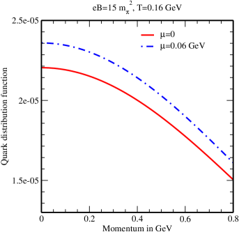
a	b

Figure 1: Variations of the quark distribution function with momentum at low temperature in the (a) absence and (b) presence of strong magnetic field.

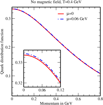
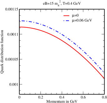
a	b

Figure 2: Variations of the quark distribution function with momentum at high temperature in the (a) absence and (b) presence of strong magnetic field.

Before proceeding to discuss the results on the transport properties and their applications in the presence of strong magnetic field and finite chemical potential, it is necessary to discuss how the distribution function behaves in the similar environment, because in kinetic theory, the distribution function in general embraces most of the information about the properties of transport coefficients. In figure 1 and figure 2, the distribution function for $u$ quark in the quasiparticle model has been plotted as a function of momentum at low temperature and high temperature, respectively. We have observed that, both in the absence and presence of strong magnetic field, the distribution function is larger at finite chemical potential in comparison to that at zero chemical potential. It is also clear that the distribution function has larger value at higher temperature (figure 2) as compared to the low temperature case (figure 1).

6 Results and discussions

In this section, we are going to discuss the results regarding electrical conductivity, thermal conductivity, Knudsen number and Wiedemann-Franz law.

6.1 Electrical conductivity

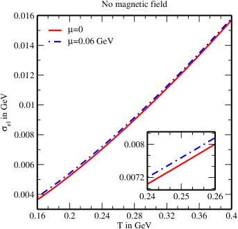
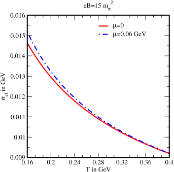
a	b

Figure 3: Variations of the electrical conductivity with temperature in the (a) absence and (b) presence of strong magnetic field.

From figure 3, we have observed that, the electrical conductivity gets enhanced in a strong magnetic field as compared to the zero magnetic field case. There are two main reasons behind this behavior of electrical conductivity, the first one is the distribution function and the second one is the dispersion relation. The strong magnetic field restricts the dynamics of charged particles to one spatial dimension (along the direction of magnetic field), which implies a stretching of the distribution function along the direction of magnetic field and a squeezing of the phase space, thus indicating a change in the dispersion relation. Therefore, the phase space integral is divided into longitudinal and transverse parts with respect to the direction of magnetic field, where the transverse part gives an overall factor of $|q_{f}B|$. In addition, the distribution functions also embody the effects of temperature and magnetic field through the effective masses in quasiparticle model. As a result, $\sigma_{\rm el}$ calculated in the strong magnetic field regime depends explicitly on magnetic field as well as temperature, whereas in the absence of magnetic field it depends only on temperature. According to the strong magnetic field (SMF) limit ($|q_{f}B|\gg T^{2}$), the energy scale associated with the magnetic field is much greater than the energy scale associated with the temperature, so $\sigma_{\rm el}$ becomes more sensitive to the magnetic field and thus electrical conductivity gets increased.

But with the rise of temperature, electrical conductivity decreases (figure 3b), contrary to its increase in the absence of magnetic field (figure 3a). This behavior of $\sigma_{\rm el}$ with temperature can be understood from the fact that, in the strong magnetic field regime, temperature is the weak energy scale, so it may leave a reverse effect on $\sigma_{\rm el}$, whereas in a pure thermal medium (i.e. in the absence of magnetic field), temperature is the dominant energy scale, so its effect on $\sigma_{\rm el}$ is more pronounced as compared to that in a strong magnetic field and the medium becomes electrically more conductive at higher temperatures.

We have also found that the finite chemical potential enhances $\sigma_{\rm el}$ both in the absence of magnetic field (figure 3a) and in the presence of strong magnetic field (figure 3b). It is well known from the nonrelativistic Drude’s formula that the electrical conductivity is directly proportional to the number density, which is the integration of distribution function over momentum space. In our case, the increase in the value of $\sigma_{\rm el}$ due to the finite chemical potential is also understood from the increase of distribution function at finite chemical potential (figures 1 and 2).

6.2 Thermal conductivity

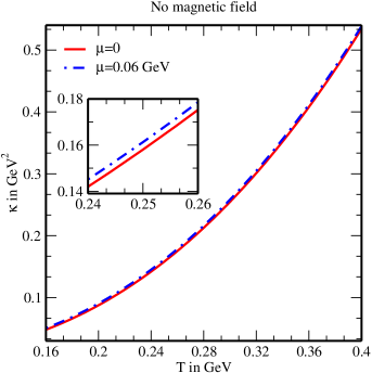
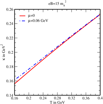
a	b

Figure 4: Variations of the thermal conductivity with temperature in the (a) absence and (b) presence of strong magnetic field.

Figure 4 shows the variations of the thermal conductivity with the temperature in the absence and in the presence of strong magnetic field and chemical potential. The presence of strong magnetic field makes $\kappa$ increased as compared to the zero magnetic field case and it shows slow increasing trend with temperature (figure 4b), contrary to its rapid increasing trend in the isotropic medium in the absence of magnetic field (figure 4a). This behavior of $\kappa$ with temperature can be understood qualitatively from the fact that the temperature is the weak energy scale in the SMF limit ($|q_{f}B|\gg T^{2}$), so its effect on $\kappa$ is meager, whereas at zero magnetic field the temperature is the strong energy scale, so its effect on $\kappa$ is abundant. The existence of finite chemical potential rises the value of $\kappa$ and this rise is more pronounced in the presence of strong magnetic field. This difference in the behavior of thermal conductivity in the absence and presence of strong magnetic field and chemical potential is attributed to the differences in the behaviors of distribution functions and the dispersion relations in the absence and presence of magnetic field and chemical potential.

6.3 Knudsen number

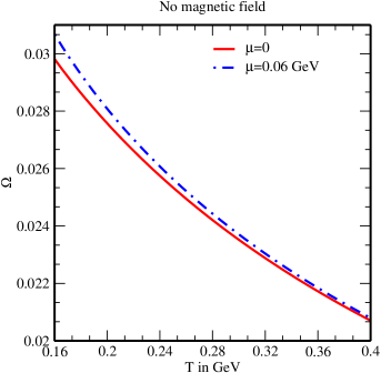
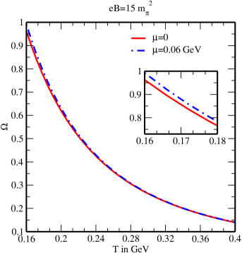
a	b

Figure 5: Variations of the Knudsen number with temperature in the (a) absence and (b) presence of strong magnetic field.

From figure 5 we have found that, in the presence of strong magnetic field, the Knudsen number ($\Omega$) becomes larger than its value in the isotropic medium with no magnetic field. We have also noticed that, in the additional presence of chemical potential, the Knudsen number becomes further increased and approaches 1 near $T_{c}=0.16$ GeV (figure 5b), i.e. the mean free path gets closer to the size of the system, unlike the isotropic case in the absence of magnetic field where although $\Omega$ gets risen at finite chemical potential, but it remains much lower than unity (figure 5a). Thus, the medium moves slightly away from the local equilibrium at finite chemical potential in an ambience of strong magnetic field.

6.4 Wiedemann-Franz law

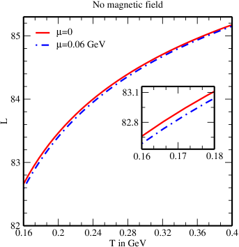
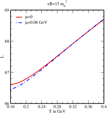
a	b

Figure 6: Variations of the Lorenz number with temperature in the (a) absence and (b) presence of strong magnetic field.

In figure 6, we have examined the validity of the Wiedemann-Franz law for a hot QCD matter in the presence of both strong magnetic field and finite chemical potential and also compared with the same in the absence of magnetic field. Figure 6a depicts the variation of the Lorenz number ($L$) with the temperature for isotropic medium in the absence of magnetic field and figure 6b depicts the same in the presence of strong magnetic field. We have noticed a decrease in the magnitude of $L$ due to the strong magnetic field as compared to the zero magnetic field case. In both the cases, finite chemical potential further reduces the magnitude of the Lorenz number, but it remains larger than unity. Thus for a hot QCD matter, thermal conductivity is much larger than its electrical conductivity at any fixed temperature; however, this difference between the thermal and electrical conducting characteristics becomes increased in the presence of a strong magnetic field and the additional presence of chemical potential further increases this difference, which also corroborate the observations on $\sigma_{\rm el}$ in figure 3 and $\kappa$ in figure 4.

We have also observed that, in all scenarios, i.e. in the absence as well as in the presence of strong magnetic field and chemical potential, with the increase of temperature, the Lorenz number does not remain constant, rather it increases. Thus, for a QCD matter, the dominance of thermal conductivity over electrical conductivity is more pronounced at higher temperatures and it explains that, the QCD matter is not a good conductor of electricity, but a very good conductor of heat, unlike some metals which are good conductors of both electricity and heat. In this perspective the QCD matter is very different from the metals. Therefore, in all abovementioned scenarios, the Wiedemann-Franz law gets violated for a hot QCD matter.

7 Conclusions

In this work, we have studied how the strong magnetic field affects the charge and thermal transport properties of the hot QCD matter at finite chemical potential and observed the deviations from their isotropic counterparts in the isotropic medium in the absence of magnetic field. In calculating the electrical and thermal conductivities we have followed the kinetic theory approach in the relaxation time approximation, where the interactions are incorporated through the effective masses of particles at finite temperature, strong magnetic field and finite chemical potential in quasiparticle model. After revisiting the calculations of electrical and thermal conductivities for the isotropic dense medium, we determined these conductivities in the presence of strong magnetic field. We have observed that the values of electrical and thermal conductivities get increased in the presence of strong magnetic field in comparison to those in the isotropic medium at zero magnetic field, and the additional presence of chemical potential further increases their values. In applications of the aforesaid conductivities, we have investigated the local equilibrium property through the Knudsen number and the relative behavior between thermal conductivity and electrical conductivity through the Lorenz number in Wiedemann-Franz law in the presence of strong magnetic field and finite chemical potential. We have observed that the Knudsen number in the presence of strong magnetic field and finite chemical potential gets increased in comparison to the isotropic one at zero magnetic field and approaches 1 around $T_{c}=0.16$ GeV, but at higher temperatures, it becomes less than 1. Thus around $T_{c}$, the mean free path gets closer to the characteristic length scale of the system and the medium may move slightly away from the local equilibrium state, whereas at higher temperatures, the medium returns back to its equilibrium state. In the Wiedemann-Franz law, the Lorenz number ($\kappa/(\sigma_{\rm el}T)$) in the absence and also in the presence of strong magnetic field and chemical potential does not remain constant, rather it increases with the rise of temperature. So, this behavior of the Lorenz number indicates the violation of the Wiedemann-Franz law for a hot and dense QCD matter in the presence of strong magnetic field.

Our observations on electrical and thermal conductivities are important from the phenomenological point of view: for large electrical conductivity, the lifetime of the strong magnetic field produced by the peripheral heavy ion collision is expected to be increased [66, 67, 68]. The emergence of chiral magnetic effect in the initial stage of the heavy ion collision is associated with the generation of current along the direction of magnetic field, which thus depends on the magnitude of the electrical conductivity [13, 69]. It was discussed that the dilepton production rate is directly proportional to the electrical conductivity of the quark-gluon plasma [70]. Thus, the enhancement of electrical conductivity due to the strong magnetic field may imply large production rate of dilepton in experiments at ultrarelativistic heavy ion collisions. In addition, it was suggested that the anisotropy of the electrical conductivity helps in the production of the elliptic flow ($v_{2}$) of the photon [71]. Our result also exhibits anisotropy due to the strong magnetic field, so it may significantly affect $v_{2}$ of the photon. Since the thermal conductivity is linked to the local equilibrium of the medium through the mean free path, its magnitude in a strong magnetic field can be used as an indicator to know how close the medium produced in peripheral heavy ion collision is to the equilibrium state in the presence of the strong magnetic field. The exploration of electrical and thermal conductivities of the hot and dense QCD matter in the strong magnetic field regime is also helpful to understand the conductive properties in other areas where strong magnetic fields might exist, such as the cores of the dense magnetars and the beginning of the universe, in addition to the ultrarelativistic heavy ion collisions.

8 Acknowledgment

One of us (B. K. P.) is thankful to the Council of Scientific and Industrial Research (Grant No. 03(1407)/17/EMR-II) for the financial assistance.

References

- [1] I. Arsene et al. (BRAHMS Collaboration), Nucl. Phys. A 757, 1 (2005); K. Adcox et al. (PHENIX Collaboration), ibid. A 757, 184 (2005); B. B. Back et al. (PHOBOS Collaboration), ibid. A 757, 28 (2005); J. Adams et al. (STAR Collaboration), ibid. A 757, 102 (2005).
- [2] F. Carminati et al. (ALICE Collaboration), J. Phys. G: Nucl. Part. Phys. 30, 1517 (2004); B. Alessandro (ALICE Collaboration), J. Phys. G: Nucl. Part. Phys. 32, 1295 (2006).
- [3] P. Senger, Cent. Eur. J. Phys. 10, 1289 (2012).
- [4] V. Skokov, A. Illarionov, and V. Toneev, Int. J. Mod. Phys. A 24, 5925 (2009).
- [5] P. Braun-Munzinger and J. Stachel, J. Phys. G 28, 1971 (2002).
- [6] J. Cleymans, J. Phys. G 35, 044017 (2008).
- [7] A. Andronic et al., Nucl. Phys. A 837, 65 (2010).
- [8] K. Fukushima and Y. Hidaka, Phys. Rev. Lett. 117, 102301 (2016).
- [9] A. Bandyopadhyay, B. Karmakar, N. Haque and M. G. Mustafa, Phys. Rev. D 100, 034031 (2019).
- [10] S. Rath and B. K. Patra, JHEP 1712, 098 (2017).
- [11] S. Rath and B. K. Patra, Eur. Phys. J. A 55, 220 (2019).
- [12] B. Karmakar, R. Ghosh, A. Bandyopadhyay, N. Haque and M. G. Mustafa, Phys. Rev. D 99, 094002 (2019).
- [13] K. Fukushima, D. E. Kharzeev and H. J. Warringa, Phys. Rev. D 78, 074033 (2008).
- [14] D. E. Kharzeev, L. D. McLerran and H. J. Warringa, Nucl. Phys. A 803, 227 (2008).
- [15] K. Tuchin, Phys. Rev. C 88, 024910 (2013).
- [16] K. A. Mamo, JHEP 1308, 083 (2013).
- [17] K. Fukushima and Y. Hidaka, JHEP 2004, 162 (2020).
- [18] K. Tuchin, Adv. High Energy Phys. 2013, 490495 (2013).
- [19] S. Rath and B. K. Patra, Phys. Rev. D 100, 016009 (2019).
- [20] Y. Hirono, M. Hongo and T. Hirano, Phys. Rev. C 90, 021903 (2014).
- [21] P. V. Buividovich, M. N. Chernodub, D. E. Kharzeev, T. Kalaydzhyan, E. V. Luschevskaya and M. I. Polikarpov, Phys. Rev. Lett. 105, 132001 (2010).
- [22] Seung-il Nam, Phys. Rev. D 86, 033014 (2012).
- [23] D. E. Kharzeev, Prog. Part. Nucl. Phys. 75, 133 (2014).
- [24] D. Satow, Phys. Rev. D 90, 034018 (2014).
- [25] S. Pu, S. Y. Wu and D. L. Yang, Phys. Rev. D 91, 025011 (2015).
- [26] K. Hattori and D. Satow, Phys. Rev. D 94, 114032 (2016).
- [27] M. Kurian and V. Chandra, Phys. Rev. D 96, 114026 (2017).
- [28] M. Kurian, S. Mitra, S. Ghosh and V. Chandra, Eur. Phys. J. C 79, 134 (2019).
- [29] J. Crossno et al., Science 351, 1058 (2016).
- [30] A. Harutyunyan, D. H. Rischke and A. Sedrakian, Phys. Rev. D 95, 114021 (2017).
- [31] S. Mitra and V. Chandra, Phys. Rev. D 96, 094003 (2017).
- [32] D. Husmann, M. Lebrat, S. Häusler, J.-P. Brantut, L. Corman and T. Esslinger, Proc. Natl. Acad. Sci. 115, 8563 (2018).
- [33] X. Han, B. Liu and J. Hu, Phys. Rev. A 100, 043604 (2019).
- [34] R. Rath, S. Tripathy, B. Chatterjee, R. Sahoo, S. K. Tiwari and A. Nath, Eur. Phys. J. A 55, 125 (2019).
- [35] L. Thakur, P. K. Srivastava, G. P. Kadam, M. George and H. Mishra, Phys. Rev. D 95, 096009 (2017).
- [36] A. Muronga, Phys. Rev. C 76, 014910 (2007).
- [37] A. Puglisi, S. Plumari and V. Greco, Phys. Rev. D 90, 114009 (2014).
- [38] S. Yasui and S. Ozaki, Phys. Rev. D 96, 114027 (2017).
- [39] S. Mitra and V. Chandra, Phys. Rev. D 94, 034025 (2016).
- [40] M. Greif, I. Bouras, C. Greiner and Z. Xu, Phys. Rev. D 90, 094014 (2014).
- [41] B. Feng, Phys. Rev. D 96, 036009 (2017).
- [42] S. Gupta, Phys. Lett. B 597, 57 (2004).
- [43] G. Aarts, C. Allton, A. Amato, P. Giudice, S. Hands and J.-I. Skullerud, JHEP 1502, 186 (2015).
- [44] H.-T. Ding, O. Kaczmarek and F. Meyer, Phys. Rev. D 94, 034504 (2016).
- [45] C. Crecignani and G. M. Kremer, “The Relativistic Boltzmann Equation: Theory and Applications” (Boston, Birkhiiuser, 2002).
- [46] A. Hosoya and K. Kajantie, Nucl. Phys. B 250, 666 (1985).
- [47] V. P. Gusynin and A. V. Smilga, Phys. Lett. B 450, 267 (1999).
- [48] V. P. Gusynin, V. A. Miransky and I. A. Shovkovy, Nucl. Phys. B 462, 249 (1996).
- [49] F. Bruckmann, G. Endrődi, M. Giordano, S. D. Katz, T. G. Kovács, F. Pittler and J. Wellnhofer, Phys. Rev. D 96, 074506 (2017).
- [50] K. Hattori, S. Li, D. Satow and H.-U. Yee, Phys. Rev. D 95, 076008 (2017).
- [51] M. Greif, F. Reining, I. Bouras, G. S. Denicol, Z. Xu and C. Greiner, Phys. Rev. E 87, 033019 (2013).
- [52] K. Fukushima, Phys. Lett. B 591, 277 (2004).
- [53] S. K. Ghosh, T. K. Mukherjee, M. G. Mustafa and R. Ray, Phys. Rev. D 73, 114007 (2006).
- [54] H. Abuki and K. Fukushima, Phys. Lett. B 676, 57 (2009).
- [55] N. Su and K. Tywoniuk, Phys. Rev. Lett. 114, 161601 (2015).
- [56] W. Florkowski, R. Ryblewski, N. Su and K. Tywoniuk, Phys. Rev. C 94, 044904 (2016).
- [57] V. M. Bannur, JHEP 0709, 046 (2007).
- [58] E. Braaten and R. D. Pisarski, Phys. Rev. D 45, R1827 (1992).
- [59] A. Peshier, B. Kämpfer and G. Soff, Phys. Rev. D 66, 094003 (2002).
- [60] M. A. Andreichikov, V. D. Orlovsky and Yu. A. Simonov, Phys. Rev. Lett. 110, 162002 (2013).
- [61] E. J. Ferrer, V. de la Incera and X. J. Wen, Phys. Rev. D 91, 054006 (2015).
- [62] A. Ayala et al., Phys. Rev. D 98, 031501 (2018).
- [63] S. Rath and B. K. Patra, arXiv:2001.11788 [hep-ph].
- [64] J. Schwinger, Phys. Rev. 82, 664 (1951).
- [65] Wu-yang Tsai, Phys. Rev. D 10, 2699 (1974).
- [66] K. Tuchin, Phys. Rev. C 88, 024911 (2013).
- [67] L. McLerran and V. Skokov, Nucl. Phys. A 929, 184 (2014).
- [68] X.-G. Huang, Rep. Prog. Phys. 79, 076302 (2016).
- [69] J. Zhao and F. Wang, Prog. Part. Nucl. Phys. 107, 200 (2019).
- [70] G. D. Moore and J.-M. Robert, arXiv:hep-ph/0607172.
- [71] Y. Yin, Phys. Rev. C 90, 044903 (2014).