Regular Model Checking Revisited

Abstract

In this contribution we revisit regular model checking, a powerful framework — pioneered by Bengt Jonsson et al. — that has been successfully applied for the verification of infinite-state systems, especially parameterized systems (concurrent systems with an arbitrary number of processes). We provide a reformulation of regular model checking with length-preserving transducers in terms of existential second-order theory over automatic structures. We argue that this is a natural formulation that enables us to tap into powerful synthesis techniques that have been extensively studied in the software verification community. More precisely, in this formulation the first-order part represents the verification conditions for the desired correctness property (for which we have complete solvers), whereas the existentially quantified second-order variables represent the relations to be synthesized. We show that many interesting correctness properties can be formulated in this way, examples being safety, liveness, bisimilarity, and games. More importantly, we show that this new formulation allows new interesting benchmarks (and old regular model checking benchmarks that were previously believed to be difficult), especially in the domain of parameterized system verification, to be solved.

1 Introduction

Verification of infinite-state systems has been an important area of research in the past few decades. This is one of the (many) areas to which Bengt Jonsson has made significant research contributions. In the late 1990s and early 2000s, an important stride advancing the verification of infinite-state systems was made when Jonsson et al. spearheaded the development of an elegant, simple, but powerful framework for modelling and verifying infinite-state systems, which they dubbed regular model checking, e.g., [1, 25, 12, 2, 3].

Regular model checking, broadly construed, is the idea of reasoning about infinite-state systems using regular languages as symbolic representations. This means that configurations of the infinite systems are encoded as finite words over some finite alphabet $\Sigma$, while other important infinite sets (e.g. of initial and final configurations) will be represented as regular languages over $\Sigma$. The transition relation $\Delta\subseteq\Sigma^{*}\times\Sigma^{*}$ of the system is, then, represented as a finite-state transducer of some sort.

Example 1

As a simple illustration, we have a unidirectional token passing protocol with $n$ processes $p_{1},\ldots,p_{n}$ arranged in a linear array. Here $n$ is a parameter, regardless of whose value (so long as it is a positive integer) the correctness property has to hold. This is also one reason why such systems are referred to as parameterized systems. Multiple tokens might exist at any given time, but at most one is held by a process. At each point in time, a process holding a token can pass it to the process to its right. If a process holding a token receives a token from its left neighbor, then it discards one of the two tokens. Each configuration of the system can be encoded as a word $w_{1}\cdots w_{n}$ over $\Sigma=\{\top,\bot\}$, where $w_{i}=\top$ (resp. $w_{i}=\bot$) denotes that process $p_{i}$ holds (resp. does not hold) a token. The set of all configurations is, therefore, $\Sigma^{*}$, i.e., a regular language. Various correctness properties can be mentioned for this system. An example of a safety property is that if the system starts with a configuration in $\top\bot^{*}$ (i.e. with only one token), then it will never visit a configuration in $\Sigma^{*}\top\Sigma^{*}\top\Sigma^{*}$ (i.e. with at least two tokens). An example of a liveness property is that it always terminates with configurations in the regular set $\bot^{*}(\bot+\top)$. ∎

This basic idea of regular model checking was already present in the work of Pnueli et al. [27] and Boigelot and Wolper [47]. However, a lot of the major development of regular model checking — the term which Jonsson et al. coined in [12] — was spearheaded by Jonsson et al.. These include fundamental contributions to acceleration techniques (including the first [25, 12]) for reachability sets and reachability relations, which could successfully verify interesting examples from parameterized systems. His works have made the works of subsequent researchers in regular model checking (including the authors of the present paper) possible. A lot of the initial work in regular model checking focussed on developing scalable algorithms (mostly via acceleration and widening) for verifying safety, while unfortunately going beyond safety (e.g. to liveness) posed a significant challenge; see [3, 45]. It is now 20 years since the publication of Jonsson’s seminal paper [12] on regular model checking. The area of computer-aided verification has undergone some paradigm shifts including the rise of SAT-solvers and SMT-solvers (e.g. see the textbooks [13, 28]), as well as synthesis algorithms [5]. In the meantime, regular model checking was also affected by this in some fashion. In 2013 Neider and Jansen [37] proposed an automata synthesis algorithm for verifying safety in regular model checking using SAT-solvers to guide the search of an inductive invariant. This new way of looking at regular model checking has inspired a new class of regular model checking algorithms, which could solve old regular model checking benchmarks that could not be solved automatically by any known automatic techniques (e.g. liveness, even for probabilistic distributed protocols [34, 30]), as well as new correctness properties (e.g. safety games [38] and probabilistic bisimulation with applications to proving anonymity [24]). Despite these recent successes, these techniques are rather ad-hoc, and often difficult to adapt to new correctness properties.

Contributions.

We provide a new and clean reformulation of regular model checking inspired by deductive verification. More precisely, we show how to express RMC as satisfaction of existential second-order logic (ESO) over automatic structures. Among others, this new framework puts virtually all interesting correctness properties (e.g. safety, liveness, safety games, bisimulation, etc.) in regular model checking under one broad umbrella. We provide new automata synthesis algorithms for solving any regular model checking problem that is expressible in this framework.

In deductive verification, we encode correctness properties of a program as formulas in some (first-order) logic, commonly called verification conditions, and then check the conditions using a theorem prover. This approach provides a clean separation of concerns between generating and checking “correctness proofs,” and underlies several verification methodologies and systems, for instance in deductive verification (with systems like Dafny [29] or KeY [4]) or termination checkers (e.g., AProVE [21] or T2 [14]). For practical reasons, the most attractive case is of course the one where all verification conditions can be kept within decidable theories. We propose to use first-order logic over universal automatic structures [9, 10, 8, 15] for the decidable theories expressing the verification conditions. Furthermore, we show that the correctness properties can be shown as satisfactions of ESO formulas over automatic structures, where the second-order variables express the existence of proofs such that the verification conditions are satisfied. Finally, we show that restricting to regular proofs (i.e. proofs that can be expressed by finite automata) is sufficient in practice, and allows us to have powerful verification algorithms that unify the recent successful automata synthesis algorithms [37, 34, 30, 24] for safety, liveness, reachability games, and other interesting correctness properties.

Organization.

Section 2 contains preliminaries. We provide our reformulation of regular model checking in terms of existential second-order logic (ESO) over automatic structures in Section 3. We provide a synthesis algorithm for solving formulas in ESO over automatic structures in Section 4. We conclude in Section 5 with research challenges.

2 Preliminaries

2.1 Automata

We assume basic familiarity with finite automata (e.g. see [41]). We use $\Sigma$ to denote a finite alphabet. In this paper, we exclusively deal with automata over finite words, but the framework and techniques extend to other classes of structures (e.g. trees) and finite automata (e.g. finite tree automata). An automaton over $\Sigma$ is a tuple $\mathcal{A}=(Q,\Delta,q_{0},F)$, where $Q$ is a finite set of states, $\Delta\subseteq Q\times Q$ is the transition relation, $q_{0}\in Q$ is the initial state, and $F\subseteq Q$ is the set of final states. In this way, our automata are by default assumed to be non-deterministic. The notion of runs of $\mathcal{A}$ on an input word $w\in\Sigma^{*}$ is standard (i.e., a function $\pi:\{0,\ldots,|w|\}\to Q$ so that $\pi(0)=q_{0}$, $\pi(|w|)\in F$, and the transition relation $\Delta$ is respected. We use $\mathcal{L}(\mathcal{A})$ to denote the language (i.e. subset of $\Sigma^{*}$) accepted by $\mathcal{A}$.

2.2 Regular Model Checking

Regular Model Checking (RMC) is a generic symbolic framework for modelling and verifying infinite-state systems pioneered and advanced by Jonsson et al. [25, 12, 3]. The basic principle behind the framework is to use finite automata to represent an infinite-state system, and witnesses for a correctness property. For example, an infinite set of states can be represented as a regular language over $\Sigma^{*}$. How do we represent a transition relation $\to\ \subseteq\Sigma^{*}\times\Sigma^{*}$? In the basic setting (as described in the seminal papers [25, 12] of Jonsson), we can use length-preserving transducers for representing $\to$. A length-preserving transducer $\mathcal{A}$ is simply an automaton over the alphabet $\Sigma\times\Sigma$. Given an input tuple $t=(u_{1}\cdots u_{n},v_{1}\cdots v_{n})\in\Sigma^{n}\times\Sigma^{n}$, an acceptance of $t$ by $\mathcal{A}$ is defined to be the acceptance of the “product” word $(u_{1},v_{1})\cdots(u_{n},v_{n})\in(\Sigma\times\Sigma)^{n}$ by the automaton $\mathcal{A}$. In this way, a transition relation $\to$ can now be represented by an automaton.

In this paper, we will deal mostly with systems whose transition relations can be represented by length-preserving transducers. This is not a problem in practice because this is already applicable for a lot of applications, including reasoning about distributed algorithms (arguably the most important class of applications of RMC), where the number of processes is typically fixed at runtime. That said, we will show how to easily extend the definition to non-length-preserving relations (called automatic relations [9, 10, 8, 15]) since they are needed in our decidable logic. This is done by the standard trick of padding the shorter strings with a special padding symbol. More precisely, given two words $v=v_{1}\cdots v_{n}$ and $w=w_{1}\cdots w_{m}$, we define the convolution $v\otimes w$ to be the word $u=(u_{1},u_{1}^{\prime})\cdots(u_{k},u_{k}^{\prime})\in(\Sigma_{\bot}\times\Sigma_{\bot})^{*}$ (where $\Sigma_{\bot}:=\Sigma\cup\{\bot\}$ and $\bot\notin\Sigma$) such that $k=\max(n,m)$, $u_{i}=v_{i}$ for all $i\leq|v|$ (for $i>|v|$, $u_{i}:=\bot$), and $u_{i}^{\prime}=w_{i}$ for all $i\leq|w|$ (for all $i>|w|$, $u_{i}^{\prime}=\bot$). For example, $ab\otimes abba$ is the word $(a,a)(b,b)(\bot,b)(\bot,a)$. Whether $(v,w)$ is accepted by $\mathcal{A}$ now is synonymous with acceptance of $v\otimes w$ by $\mathcal{A}$. In this way, transition relations that relate words of different lengths can still be represented using finite automata.

2.3 Weakly-Finite Systems

In this paper, we will restrict ourselves to transition systems whose domain is a regular subset of $\Sigma^{*}$, and whose transition relations can be described by length-preserving transducers. That is, since $\Sigma$ is finite, from any given configuration $w\in\Sigma^{*}$ of the system there is a finite number of configurations that are reachable from $w$ (in fact, there is at most $|\Sigma|^{|w|}$ reachable configurations). Such transition systems (which can be infinite, but where the number of reachable configurations from any given configuration is finite) are typically referred to as weakly-finite systems [19]. As we previously mentioned, this restriction is not a big problem in practice since many practical examples (including those from distributed algorithms) can be captured. The restriction is, however, useful when developing a clean framework that is unencumbered by a lot of extra assumptions, and at the same time captures a a lot of interesting correctness properties.

2.4 Existential Second-Order Logic

In this paper, we will use Existential Second-Order Logic (ESO) to reformulate RMC. Second-order Logic (e.g. see [31]) is an extension of first-order logic by quantifications over relations. Let $\sigma$ be a vocabulary consisting of relations (i.e. relational vocabulary). A relational variable will be denoted by capital letters $R,X,Y$, etc. Each relational variable $R$ has an arity $\text{{ar}}(R)\in\mathbb{Z}_{>0}$. ESO over $\sigma$ is simply the fragment of second-order logic over $\sigma$ consisting of formulas of the form

$$\psi=\exists R_{1},\ldots,R_{n}.\,\varphi$$

where $\varphi$ is a first-order logic over the vocabulary $\sigma^{\prime}=\sigma\cup\{R_{i}\}_{i=1}^{n}$, where $R_{i}$ is a relation symbol of arity $\text{{ar}}(R_{i})$. Given a structure $\mathfrak{S}$ over $\sigma$ and an ESO formula $\psi$ (as above), checking whether $\mathfrak{S}\models\psi$ amounts to finding relations $R_{1},\ldots,R_{n}$ over the domain of $\mathfrak{S}$ such that $\varphi$ is satisfied (with the standard definition of first-order logic); in other words, extending $\mathfrak{S}$ to a structure $\mathfrak{S}^{\prime}$ over $\sigma^{\prime}$ such that $\mathfrak{S}^{\prime}\models\varphi$.

3 RMC as ESO Satisfaction over Automatic Structures

As we previously described, our new reformulation of RMC is inspired by deductive verification, which provides a separation between generating and checking correctness proofs. The verification conditions should be describable in decidable logical theories. As a concrete example, suppose we want to prove a safety property for a program $P$. Then, a correctness proof would be a finitely-representable inductive invariant $\mathit{Inv}$ that contains all initial states of $P$, and is disjoint from the set of all bad states of $P$. The termination of a program can similarly be proven by finding a well-founded relation $\mathit{Rank}$ that subsumes the transition relation of a program. In both cases, a correctness proof corresponds to a solution for existentially quantified second-order variables that encode the desired correctness property; in the spirit of Section 2.4, the correctness of a proof can be verified by evaluating just the first-order part $\varphi$ of a formula. The generation of the candidate proofs will then be taken care of separately, which we will talk about in the next section. Suffice to say for now that the counterexample guided inductive synthesis (CEGIS) framework [5] would be appropriate for the proof generation. In this section, we provide a reformulation of RMC in the aforementioned framework for software verification.

3.1 Automatic Structures

What is the right decidable theory to capture regular model checking? We venture that the answer is the first-order theory of an automatic structure [9, 10, 8, 15]. An automatic structure over the vocabulary consisting of relations $R_{1},\ldots,R_{n}$ with arities $r_{1},\ldots,r_{n}$ is a structure $\mathfrak{S}$ whose universe is the set $\Sigma^{*}$ of all strings over some finite alphabet $\Sigma$, and where each relation $R_{i}\subseteq(\Sigma^{*})^{r_{i}}$ is regular, i.e., the set $\{w_{1}\otimes\cdots\otimes w_{r_{i}}:(w_{1},\ldots,w_{r})\in R_{i}\}$ is regular. The following well-known closure and algorithmic property is what makes the theory of automatic structures appealing.

Theorem 3.1

There is an algorithm which, given a first-order formula $\varphi(\bar{x})$ and an automatic structure $\mathfrak{S}$ over the vocabulary $\sigma$, computes a finite automaton for $[\![\varphi]\!]$ consisting of tuples $\bar{w}$ of words, such that $\mathfrak{S}\models\varphi(\bar{w})$.

The algorithm is a standard automata construction (e.g. see [42] for details), which is indeed similar to the standard automata construction from the weak second-order theory of one successor [22]. [In fact, first-order logic over automatic structures can be encoded (and vice versa) to weak second-order theory of one successor via the so-called finite set interpretations [18], which would allow us to use tools like MONA to check first-order formulas over automatic structures.]

Automatic structures are extremely powerful. We can encode the linear integer arithmetic theory $\langle{\mathbb{N}};+\rangle$ as an automatic structure [15]. In fact, we can even add the predicate $x|_{2}y$ (where $a|_{2}b$ iff $a$ divides $b$ and $a=2^{n}$ for some natural number $n$) to $\langle{\mathbb{N}};+\rangle$, while still preserving decidability. This essentially implies that ESO over automatic structures is undecidable; in fact, this is the case even when formulas are restricted to monadic predicates.

We are now ready to describe our framework for RMC in ESO over automatic structures:

1. Specification:
   Express the verification problem as a formula

   $$\psi:=\exists R_{1},\ldots,R_{n}.\,\varphi$$

   in ESO over automatic structures.

2. Specification Checking:
   Search for regular witnesses for $R_{1},\ldots,R_{n}$ that satisfy $\varphi$.

Note that while the specification (Item (i)) would provide a complete and faithful encoding of the verification problem, our method for checking the specification (Item (ii)) restricts to regular proofs. It is expected that this is an incomplete proof rule, i.e., for $\psi$ to be satisfied, it is not sufficient in general to restrict to regular relations. Therefore, two important questions arise. Firstly, how expressive is the framework of regular proofs? Numerous results suggest that the answer is that it is very expressive. On the practical side, many benchmarks (especially from parameterized systems) have indicated this to be the case, e.g., see [37, 17, 34, 30, 38, 3, 45, 39, 24, 33]. On the theoretical side, this framework is in fact complete for important properties like safety and liveness for many classes of infinite-state systems that can be captured by regular model checking, including pushdown systems, reversal-bounded counter systems, two-dimensional vector addition systems, communication-free Petri nets, and tree-rewrite systems (for the extension to trees), among others, e.g., see [42, 43, 7, 32, 23, 35]. In addition, the restriction to regular proofs is also attractive since it gives rise to a simple method to enumerate all regular proofs that check $\varphi$. This naive method would not work in practice, but smart enumeration techniques of regular proofs (e.g., using automata learning and CEGIS) are available, which we will discuss in Section 4.

3.2 Safety

We start with the most straightforward example: safety. We assume that our transition system is represented by a length-preserving system with domain $\mathit{Dom}\subseteq\Sigma^{*}$ and a transition relation $\Delta\subseteq\mathit{Dom}\times\mathit{Dom}$ given by a length-preserving transducer. Furthermore, we assume that the system contains two regular languages $\mathit{Init},\mathit{Bad}\subseteq\mathit{Dom}$, representing the set of initial and bad states. As we mentioned earlier in this section, safety amounts to checking the existence of an invariant $\mathit{Inv}\subseteq\mathit{Dom}$ that contains $\mathit{Init}$ but is disjoint from $\mathit{Bad}$. That is, the safety property holds iff there exists a set $\mathit{Inv}\subseteq\mathit{Dom}$ such that:

• $\mathit{Init}\subseteq\mathit{Inv}$

• $\mathit{Inv}\cap\mathit{Bad}=\emptyset$

• $\mathit{Inv}$ is inductive, i.e., for every configuration $s\in\mathit{Inv}$, if $(s,s^{\prime})\in\Delta$, then $s^{\prime}\in\mathit{Inv}$.

The above formulation immediately leads to a first-order formula $\varphi$ over the vocabulary of $\langle\Delta,\mathit{Init},\mathit{Bad},\mathit{Inv}\rangle$. Therefore, the desired ESO formula over the original vocabulary (i.e. $\langle\Delta,\mathit{Init},\mathit{Bad}\rangle$) is

$$\exists\mathit{Inv}.\,\varphi,$$

where $\varphi$ is a conjunction of the three properties above.

Example 2

Fix $\Sigma=\{0,1\}$. Consider the transition relation $\Delta\subseteq\Sigma^{*}\times\Sigma^{*}$ generated by the regular expression $((0,0)+(1,1))^{*}(1,0)(0,1)((0,0)+(1,1))^{*}$. Intuitively, $\Delta$ nondeterministically picks a substring 10 in an input word $w$ and rewrites it to 01. Let $\mathit{Init}=0\Sigma^{*}1$ and $\mathit{Bad}=1^{*}0^{*}$. Observe that there is a regular proof $\mathit{Inv}$ for this safety property: $\mathit{Inv}=\mathit{Init}$. Note that this is despite the fact that $post^{*}(\mathit{Init})$ in general is not a regular set.

3.3 Liveness

A second class of properties are liveness properties, for instance checking whether a program is guaranteed to terminate, guaranteed to answer requests eventually, or guaranteed to visit certain states infinitely often. In the context of RMC, liveness has been studied a lot less than safety, and methods sucessful for proving safety usually do not lend themselves to an easy generalisation to liveness.

For simplicity, the special case of program termination is consider, which can be generalized to full liveness. As before, we assume that a transition system is defined by a domain $\mathit{Dom}\subseteq\Sigma^{*}$, a transition relation $\Delta\subseteq\mathit{Dom}\times\mathit{Dom}$, and a set $\mathit{Init}\subseteq\mathit{Dom}$ of initial states. Proving termination amounts to showing that no infinite runs starting from a state in $\mathit{Init}$ exist; to this end, we can search for a pair $\langle\mathit{Inv},\mathit{Rank}\rangle$ consisting of an inductive invariant and a well-founded ranking relation:

• $\mathit{Init}\subseteq\mathit{Inv}$;

• $\mathit{Inv}$ is inductive (as in Section 3.2);

• the relation $\mathit{Rank}$ covers the reachable transitions: $\Delta\cap(\mathit{Inv}\times\mathit{Inv})\subseteq\mathit{Rank}$;

• $\mathit{Rank}$ is transitive: $(s,s^{\prime})\in\mathit{Rank}$ and $(s^{\prime},s^{\prime\prime})\in\mathit{Rank}$ imply $(s,s^{\prime\prime})\in\mathit{Rank}$;

• $\mathit{Rank}$ is irreflexive: $(s,s)\not\in\mathit{Rank}$ for every $s\in\mathit{Dom}$.

The last two conditions ensure that $\mathit{Rank}$ is a strict partial order, and therefore is even well-founded on fixed-length subsets $\mathit{Dom}\cap\Sigma^{n}$ of the domain. All five conditions can easily be expressed by a first-order formula $\varphi$ over the relations $\langle\Delta,\mathit{Init},\mathit{Inv},\mathit{Rank}\rangle$. Now, for length-preserving relations $R$, expressing in first-order logic that a transitive relation is well-founded is simple: it is not the case that there are words $x,y$ such that $(x,y)\in R$ and $(y,y)\in R$. This “lasso” shape is owing to the fact that in every finite system every infinite path always leads to one state that is visited infinitely often. In summary, termination of a system is therefore captured by the following ESO formula:

$$\exists\mathit{Inv},\mathit{Rank}.\,\varphi~{}$$

where $\varphi$ is the first-order part that encodes the aforementioned verification conditions.

Example 3

We consider here the same example as Example 2, but we instead want to prove termination. It is quite easy to see that every configuration will always lead to a configuration of the form $0^{*}1^{*}$, which is a dead end. Termination of the system can be proven using the trivial inductive invariant $\mathit{Inv}=\mathit{Dom}$, and a lexicographic ranking relation $\mathit{Rank}$, represented as a transducer with two states and shown in Fig. 1. Using the algorithms proposed in Section 4, this ranking relation can be computed fully automatically in a few milliseconds.

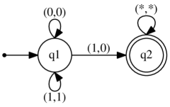
Figure 1: Lexicographic ranking relation for Example 3

3.4 Winning Strategies for Two-Player Games on Infinite Graphs

We only need to slightly modify the ESO formula for program termination, given in the previous section, to reason about the existence of winning strategies in a reachability game. Instead of a single transition relation $\Delta$, for a two-player game we assume that two relations $\Delta_{1},\Delta_{2}\subseteq\mathit{Dom}\times\mathit{Dom}$ are given, encoding the possible moves of Player 1 and Player 2, respectively. A reachability game starts in any configuration in the set $\mathit{Init}\subseteq\mathit{Dom}$. The players move in alternation, with Player 2 winning if the game eventually reaches a configuration in $\mathit{Final}\subseteq\mathit{Dom}$, whereas Player 1 wins if the game never enters $\mathit{Final}$. The first move in a game is always done by Player 1.

As in the previous section, we formulate the existence of a winning strategy for Player 2 (for any initial configuration in $\mathit{Init}$) in terms of a pair $\langle\mathit{Inv},\mathit{Rank}\rangle$ of relations. The set $\mathit{Inv}$ now represents the possible configurations that Player 1 visits during games, whereas the ranking relation $\mathit{Rank}$ expresses progress made by Player 2 towards the region $\mathit{Final}$.

• $\mathit{Init}\subseteq\mathit{Inv}$;

• $\mathit{Rank}$ is transitive and irreflexive (as in Section 3.3);

• Player 2 can force the game to progress: for every $s\in\mathit{Inv}\setminus\mathit{Final}$, and every move $(s,s^{\prime})\in\Delta_{1}$ of Player 1 with $s^{\prime}\not\in\mathit{Final}$, there is a move $(s^{\prime},s^{\prime\prime})\in\Delta_{2}$ of Player 2 such that $s^{\prime\prime}\in\mathit{Inv}$ and $(s,s^{\prime\prime})\in\mathit{Rank}$.

It is again easy to see that all conditions can be expressed by a first-order formula over the relations $\langle\Delta_{1},\Delta_{2},\mathit{Init},\mathit{Final},\mathit{Inv},\mathit{Rank}\rangle$, and the existence of a winning strategy as an ESO formula:

$$\exists\mathit{Inv},\mathit{Rank}.\,\varphi~{}.$$

A similar encoding has been used in previous work of the authors to reason about almost-sure termination of parameterised probabilistic systems [34, 30]. In this setting, the two players characterise non-determinism (demonic choice, e.g., the scheduler) and probabilistic choice (angelic choice, e.g., randomisation).

Example 4

We consider a classical take-away game [20] with two players. In the beginning of the game, there are $n$ chips on the table. In alternating moves, with Player 1 starting, each player can take 1, 2, or 3 chips from the table. The first player who has no more chips to take loses. It can be observed that Player 2 has a winning strategy whenever the initial number $n$ is a multiple of $4$.

Configurations of this game can be modelled as words $(p_{1}+p_{2})1^{*}0^{*}$, in which the first letter ($p_{1}$ or $p_{2}$) indicates the next player to make a move, and the number of $1$s represents the number of chips left. To prove that Player 2 can win whenever $n=4k$, we choose $\mathit{Init}=p_{1}(1111)^{*}0^{*}$ as the initial states, and $\mathit{Final}=p_{1}0^{*}$, i.e., we check whether Player 2 can move first to a configuration in which no chips are left. The transitions of the two players are described by the regular expressions

$$\Delta_{1} ~{}=~{}(p_{1},p_{2})\,(1,1)^{*}\,\big{(}(1,0)+(11,00)+(111,000)\big{)}\,(0,0)^{*}$$

$$\Delta_{2} ~{}=~{}(p_{2},p_{1})\,(1,1)^{*}\,\big{(}(1,0)+(11,00)+(111,000)\big{)}\,(0,0)^{*}$$

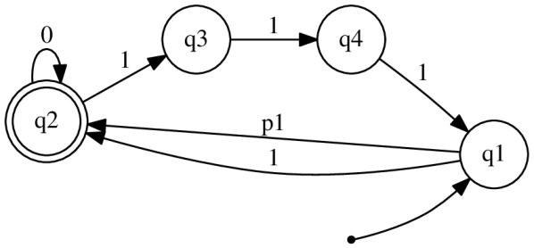
Figure 2: Set $\mathit{Inv}$ of reachable configurations of the take-away game in Example 4

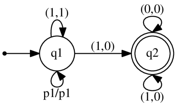
Figure 3: Relation $\mathit{Rank}$ in Example 4

The witnesses proving that Player 2 indeed has a winning strategy are shown in Fig. 3 and Fig. 3, respectively. The ranking relation $\mathit{Rank}$ in Fig. 3 is similar to the one proving termination in Example 3, and expresses that the number of $1$s is monotonically decreasing. The invariant $\mathit{Inv}$ in Fig. 3 expresses that Player 2 should move in such a way that the number of chips on the table remains divisible by $4$; $\mathit{Rank}$ and $\mathit{Inv}$ in combination encode the strategy that Player 2 should follow to win. The witness relations were found by the tool SLRP, presented in [34], in around 3 seconds on an Intel Core i5 computer with 3.2 GHz.

3.5 Isomorphism and Bisimulation

We now describe how we can compare the behaviour of two given systems described by length-preserving transducers. There are many natural notions of “similarity”, but we target isomorphism, bisimulation, and probabilistic bisimulation (or variants thereof). All of these are important properties since they show indistinguishability of two systems, which are applicable to proving anonymity, e.g., in the case of the Dining Cryptographer Protocol [16]. Isomorphism can also be used to detect symmetries in systems, which can be used to speed up regular model checking [33]. Here, we only describe how to express isomorphism of two systems. Encoding bisimulation and probabilistic bisimulation for parameterized systems is a bit trickier since we will need infinitely many action labels (i.e. to distinguish the action of the $i$th process), but this can also be encoded in our framework; see the first-order proof rules over automatic structures in the recent paper [24].

We are given two systems $\mathfrak{S}_{1}$, $\mathfrak{S}_{2}$, whose domains are $Dom_{1},Dom_{2}\subseteq\Sigma^{*}$ and whose transition relations $R_{1}$ and $R_{2}$ are described by transducers. We would like to show that $\mathfrak{S}_{1}$ and $\mathfrak{S}_{2}$ are the same up to isomorphism. The desired ESO formula is of the form

$$\exists F.\,\varphi$$

where $\varphi$ says that $F\subseteq Dom_{1}\times Dom_{2}$ describes the desired isomorphism between $\mathfrak{S}_{1}$ and $\mathfrak{S}_{2}$. To this end, we will first need to say that $F$ is a bijective function. This can easily be described in first-order logic over the vocabulary $\langle Dom_{1},Dom_{2},R_{1},R_{2}\rangle$. For example, $F$ is a function can be described as

$$\forall x,y,z.\,(F(x,y)\wedge F(x,z)\to y=z).$$

Note that $y=z$ can be described by a simple transducer, so this is a valid first-order formula over automatic structures. We then need to add some more conjuncts in $\varphi$ saying that $F$ is a homomorphism and its reverse is also a homomorphism. This is also easily described in first-order logic, e.g.,

$$\forall x,x^{\prime},y,y^{\prime}.\,(R_{1}(x,y)\wedge F(x,x^{\prime})\wedge F(y,y^{\prime})\to R_{2}(x^{\prime},y^{\prime}))$$

says that $F$ is a homomorphism.

Example 5

We describe the Dining Cryptographer example [16], and how to prove this by reasoning about isomorphism. [There is a cleaner way to do this using probabilistic bisimulation [24].] In this protocol there are $n$ cryptographers sitting at a round table. The cryptographers knew that the dinner was paid by NSA, or exactly one of the cryptographers at the table. The protocol aims to determine which one of these without revealing the identity of the cryptographer who pays. The $i$th cryptographer is in state $c_{i}=0$ (resp. $c_{i}=1$) if he did not pay for the dinner. Any two neighbouring cryptographers keep a private fair coin (that is only visible to themselves). There is a transition to toss any of the coins (in this case, probability is replaced by non-determinism). Let us use $p_{i}$ to denote the value of the coin that is shared by the $i$th and $i+1\pmod{n}$st cryptographers. If the $i$th cryptographer paid, it will announce $p_{i-1}\oplus p_{i}$ (here $\oplus$ is the XOR operator); otherwise, it will announce the negation of this. We call the value announced by the $i$th cryptographer $a_{i}$. At the end, we take the XOR of $a_{1},\ldots,a_{n}$, which is 0 iff none of the cryptographers paid.

This example can easily be encoded by a length-preserving transducer $R$. For example, the domain is a word of the form

$$(c_{1}p_{1}a_{1})\ldots(c_{n}p_{n}a_{n})$$

where $c_{i}\in\{0,1\}$ and $p_{i},a_{i}\in\{?,0,1\}$. Here, the symbol ’?’ is used to denote that the value of $p_{i}$ is not yet determined. In the case of $a_{i}$, the symbol ’?’ means that it is not yet announced. Although it is a bit cumbersome, it is possible to describe the dynamics of the system by a transducer. The desired property to prove then is whether there is an isomorphism between $0100^{m}$ and $0010^{m}$ for every $m\in{\mathbb{N}}$, i.e., that the first cryptographer, who did not pay, cannot distinguish if it were the second or the third cryptographer who paid. There is a transducer $R^{\prime}$ describing the isomorphism that maps $0100^{m}$ to $0010^{m}$, which is done by inverting the value of $p_{2}$.

4 How to Satisfy Existential Second-Order Quantifiers

We have given several examples for the Specification step in Section 3.1, but the question remains how one can solve the Specification Checking step and automatically compute witnesses $R_{1},\ldots,R_{n}$ for the existential quantifiers in a formula $\exists R_{1},\ldots,R_{n}.\,\varphi$ (where the matrix $\varphi$ is first-order, as introduced in Section 2.4). We present two solutions for this problem, two approaches to automata learning whose respective applicability depends on the shape of the matrix $\varphi$. Both methods have in previous work proven to be useful for analysing complex parameterised systems. On the one hand, it has been shown that automata learning is competitive with tailor-made algorithms, for instance with Abstract Regular Model Checking (ARMC) [11], for safety proofs [44, 17]; on the other hand, automata learning is general and can help to automate the verification of properties for which no bespoke approaches exist, for instance liveness properties or properties of games.

4.1 Active Automata Learning

The more efficient, though also more restricted approach is to use classical automata learning, for instance Angluin’s $L^{*}$ algorithm [6], or one of its variants (e.g., [40, 26]), to compute witnesses for $R_{1},\ldots,R_{n}$. In all those algorithms, a learner attempts to reconstruct a regular language $\cal L$ known to the teacher by repeatedly asking two kinds of queries: membership, i.e., whether a word $w$ should be in $\cal L$; and equivalence, i.e., whether $\cal L$ coincides with some candidate language $\cal H$ constructed by the learner. When equivalence fails, the teacher provides a positive or negative counterexample, which is a word in the symmetric difference between $\cal L$ and $\cal H$.

This leads to the question how membership and equivalence can be implemented in the ESO setting, in order to let a learner search for $R_{1},\ldots,R_{n}$. In general, it is clearly not possible to answer membership queries about $R_{1},\ldots,R_{n}$, since there can be many choices of relations satisfying $\varphi$, some of which might contain a word, while others do not; in other words, the relations are in general not uniquely determined by $\varphi$. We need to make additional assumptions.

As the simplest case, active automata learning can be used if two properties are satisfied: (i) the relations $R_{1},\ldots,R_{n}$ are uniquely defined by $\varphi$ and the structure $\mathfrak{S}$; and (ii) for any $k\in{\mathbb{N}}$, the sub-relations $R_{i}^{k}=\{w\in R_{i}\mid|w|\leq k\}$ can be effectively computed from $\varphi$ and $\mathfrak{S}$. Given those two assumptions, automata learning can be used to approximate the genuine solution $R_{1},\ldots,R_{n}$ up to any length bound $k$, resulting in a candidate solution $R_{1}^{\cal H},\ldots,R_{n}^{\cal H}$. It can also be verified whether $R_{1}^{\cal H},\ldots,R_{n}^{\cal H}$ coincide with the genuine solution by evaluating $\varphi$, i.e., by checking whether $\mathfrak{S},R_{1}^{\cal H},\ldots,R_{n}^{\cal H}\models\varphi$. If this check succeeds, learning has been successful; if it fails, the bound $k$ can be increased and a better approximation computed. Whenever the unique solution $R_{1},\ldots,R_{n}$ exists and is regular, this algorithm is guaranteed to terminate and produce a correct answer.

In the setting of weakly-finite systems, assumption (ii) is usually satisfied, since only finitely many configurations are reachable for any $k\in{\mathbb{N}}$. In particular, for the examples in Section 3, the sub-relations $R_{1}^{k},\ldots,R_{n}^{k}$ can be computed using standard methods such as symbolic model checking [36]. Assumption (i) is less realistic, because witnesses to be computed in verification are often not uniquely defined. For instance, a safe system (Section 3.2) will normally have many inductive invariants, each of which is sufficient to demonstrate safety.

What can be done when assumption (i) does not hold, and the relations $R_{1},\ldots,R_{n}$ are not unique? Depending on the shape of $\varphi$, a simple trick can be applicable, namely the learning algorithm can be generalised to search for a unique smallest or unique largest solution (in the set-theoretic sense) of $\varphi$, provided those solutions exist. This is the case in particular when $\varphi$ can be rephrased as a fixed-point equation

$$\langle R_{1},\ldots,R_{n}\rangle=F(R_{1},\ldots,R_{n})$$

for some monotonic function $F$; for instance, if $\varphi$ can be written as a set of Horn clauses. We still require property (ii), however, and need to be able to compute sub-relations $R_{i}^{k}=\{w\in R_{i}\mid|w|\leq k\}$ of the smallest or largest solution to answer membership queries.

In order to check whether a solution candidate $R_{1}^{\cal H},\ldots,R_{n}^{\cal H}$ is correct (for equivalence queries), we can as before evaluate $\varphi$, and terminate the search if $\varphi$ is satisfied. In general, however, there is no way to verify that $R_{1}^{\cal H},\ldots,R_{n}^{\cal H}$ is indeed the smallest solution of $\varphi$, which affects termination and completeness in a somewhat subtle way. If the smallest solution of $\varphi$ exists and is regular, then termination of the overall search is guaranteed, and the produced solution will indeed satisfy $\varphi$; but what is found is not necessarily the smallest solution of $\varphi$.

This method has been implemented in particular for proving safety [44, 17] and probabilistic bisimulations [24] of length-preserving systems, cases in which $\varphi$ is naturally monotonic, and where active learning methods are able to compute witnesses with hundreds (sometimes thousands) of states within minutes.

4.2 SAT-Based Automata Learning

$L^{*}$-style learning is not applicable if the matrix of an ESO formula $\exists R_{1},\ldots,R_{n}.\,\varphi$ does not have a smallest or largest solution, or if the sub-relations $R_{1}^{k},\ldots,R_{n}^{k}$ (for some $k\in{\mathbb{N}}$) cannot be computed because a system is not weakly finite. An example of such non-monotonic formulas are the formulas characterising winning strategies of reachability games presented in Section 3.4; indeed, multiple minimal but incomparable strategies can exist to win a game, so that in general there is no smallest solution. A more general learning strategy to solve ESO formulas in the non-monotonic case is SAT-based learning, i.e., using a Boolean encoding of finite-state automata to systematically search for solutions of $\varphi$ [37, 34, 46]. SAT-based learning is a more general solution than active automata learning for constructing ESO proofs, although experiments show that it is also a lot slower for simpler analysis tasks like safety proofs [17].

We outline how a SAT solver can be used to construct deterministic finite-state automata (DFAs), following the encoding used in [34]. The encoding assumes that a finite alphabet $\Sigma$ and the number $n$ of states of the automaton are fixed. The states of the automaton are assumed to be $q_{1},\ldots,q_{n}$, and without loss of generality $q_{1}$ is the unique initial state. The Boolean decision variables of the encoding are (i) variables $\{z_{i}\}$ that determine which of the states are accepting; and (ii) variables $\{x_{i,a,j}\}$ that determine, for any letter $a\in\Sigma$ and states $q_{i},q_{j}$, whether the automaton has a transition from $q_{i}$ to $q_{j}$ with label $a$.

A number of Boolean constraints are then asserted to ensure that only well-formed DFAs are considered: determinism; reachability of every automaton state from the initial state; reachability of an accepting state from every state; and symmetry-breaking constraints.

Next, the formula $\varphi$ can be translated to Boolean constraints over the decision variables. This translation can be done eagerly for all conjuncts of $\varphi$ that can be represented succinctly:

• a positive atom $x\in R$ in which the length of $x$ is bounded can be translated to constraints that assert the existence of a run accepting $x$;

• a negative atom $x\not\in R$ can similarly be encoded as a run ending in a non-accepting state, thanks to the determinism of the automaton;

• for automata representing binary relations $R(x,y)$, several universally quantified formulas can be encoded as a polynomial-size Boolean constraint as well, including:

  Reflexivity: $$\forall x.\,R(x,x)$$

  Irreflexivity: $$\forall x.\,\neg R(x,x)$$

  Functional consistency: $$\forall x,y,z.\,(R(x,y)\wedge R(x,z)\to y=z)$$

  Transitivity: $$\forall x,y,z.\,(R(x,y)\wedge R(y,z)\to R(x,z))$$

Other conjuncts in $\varphi$ can be encoded lazily with the help of a refinement loop, resembling the classical CEGAR approach. The SAT solver is first queried to produce a candidate automaton $\cal H$ that satisfies a partial encoding of $\varphi$. It is then checked whether the candidate $\cal H$ indeed satisfies $\varphi$; if this is the case, SAT-based learning has been successful and terminates; otherwise, a blocking constraint is asserted that rules out the candidate $\cal H$ in subsequent queries.

It should be noted that this approach can in principle be implemented for any formula $\varphi$, since it is always possible to generate a naïve blocking constraint that blocks exactly the observed assignment of the variables $\{z_{i},x_{i,a,j}\}$, i.e., that exactly matches the automaton $\cal H$. It is well-known in Satisfiability Modulo Theories, however, that good blocking constraints are those which eliminate as many similar candidate solutions as possible, and need to be designed carefully and specifically for a theory (or, in our case, based on the shape of $\varphi$).

Several implementations of SAT-based learning have been described in the literature, for instance for computing inductive invariants [37], synthesising state machines satisfying given properties [46], computing symmetries of parameterized systems [33], and for solving various kinds of games [34]. Experiments show that the automata that can be computed using SAT-based learning tend to be several order of magnitudes smaller than with active automata learning methods (typically, at most 10–20 states), but that SAT-based learning can solve a more general class of synthesis problems as well.

4.3 Stratification of ESO Formulas

The two approaches to compute regular languages can sometimes be combined. For instance, in [34] active automata learning is used to approximate the reachable configurations of a two-player game (in the sense of computing an inductive invariant), whereas SAT-based learning is used to compute winning strategies; the results of the two procedures in combination represent a solution of an ESO formula $\exists A,\mathit{Rank}.\,\varphi$ with two second-order quantifiers.

More generally, since the active automata learning approach in Section 4.1 is able to compute smallest or greatest solutions of formulas, a combined approach is possible when the matrix $\varphi$ of an ESO formula $\exists R_{1},\ldots,R_{n}.\,\varphi$ can be stratified. Suppose $\varphi$ can be decomposed into $\varphi_{1}[R_{1}]\wedge\varphi_{2}[R_{1},\ldots,R_{n}]$ in such a way that (i) $\varphi_{1}$ has a unique smallest solution in $R_{1}$, and (ii) $\varphi_{2}$ contains $R_{1}$ only in literals $x\in R_{1}$ in negative positions, i.e., underneath an odd number of negations. In this situation, one can clearly proceed by first computing a smallest relation $R_{1}$ satisfying $\varphi_{1}$, using the methods in Section 4.1, and then solve the remaining formula $\exists R_{2},\ldots,R_{n}.\,\varphi_{2}$ given this fixed solution for $R_{1}$. The case where $\varphi_{1}$ has a greatest solution, and $\varphi_{2}$ contains $R_{1}$ only positively can be handled similarly.

We believe that this combined form of automata learning is promising, and in [34] it turned out to be the most efficient method to solve reachability games as introduced in Section 3.4. Further research is needed, however, to evaluate the approach for other verification problems.

5 Conclusions

In this paper, we have proposed existential second-order logic (ESO) over automatic structures as an umbrella covering a large number of regular model checking tasks, continuing a research programme that was initiated by Bengt Jonsson 20 years ago. We have shown that many important correctness properties can be represented elegantly in ESO, and developed unified algorithms that can be applied to any correctness property captured using ESO. Experiments showing the practicality of this approach have been presented in several recent publications, including computation of inductive invariants [44, 37, 17], of symmetries and simulation relations of parameterised systems [33], of winning strategies of games [34, 30], and of probabilistic bisimulations [24].

Several challenges remain. One bottleneck that has been identified in several of the studies is the size of alphabets necessary to model systems, to which the algorithms presented in Section 4 are very sensitive. This indicates that some analysis tasks require more compact or more expressive automata representations, for instance symbolic automata, and generalised learning methods; or abstraction to reduce the size of alphabets. Another less-than-satisfactory point is the handling of well-foundedness in the ESO framework. When restricting the class of considered systems to weakly finite systems, as done here, well-foundedness of relations can be replaced by acyclicity, which can be expressed easily in ESO (as shown in Section 3.3). It is not obvious, however, in which way ESO should be extended to also handle systems that are not weakly finite, without sacrificing the elegance of the approach.

Acknowledgment.

First and foremost, we thank Bengt Jonsson for a source of inspiration for our research for many years, as well as for being the best colleague and friend one could wish for. We also thank our numerous collaborators in our work on regular model checking that led to this work, including Parosh Abdulla, Yu-Fang Chen, Lukas Holik, Chih-Duo Hong, Ondrej Lengal, Leonid Libkin, Rupak Majumdar, and Tomas Vojnar. This research was sponsored in part by the ERC Starting Grant 759969 (AV-SMP), Max-Planck Fellowship, the Swedish Research Council (VR) under grant 2018-04727, and by the Swedish Foundation for Strategic Research (SSF) under the project WebSec (Ref. RIT17-0011).

References

- [1] P. A. Abdulla, A. Bouajjani, B. Jonsson, and M. Nilsson. Handling global conditions in parameterized system verification. In Computer Aided Verification, 11th International Conference, CAV ’99, Trento, Italy, July 6-10, 1999, Proceedings, pages 134–145, 1999.
- [2] P. A. Abdulla, B. Jonsson, P. Mahata, and J. d’Orso. Regular tree model checking. In CAV, pages 555–568, 2002.
- [3] P. A. Abdulla, B. Jonsson, M. Nilsson, and M. Saksena. A survey of regular model checking. In CONCUR, pages 35–48, 2004.
- [4] W. Ahrendt, B. Beckert, R. Bubel, R. Hähnle, P. H. Schmitt, and M. Ulbrich, editors. Deductive Software Verification - The KeY Book - From Theory to Practice, volume 10001 of Lecture Notes in Computer Science. Springer, 2016.
- [5] R. Alur, R. Bodík, G. Juniwal, M. M. K. Martin, M. Raghothaman, S. A. Seshia, R. Singh, A. Solar-Lezama, E. Torlak, and A. Udupa. Syntax-guided synthesis. In Formal Methods in Computer-Aided Design, FMCAD 2013, Portland, OR, USA, October 20-23, 2013, pages 1–8, 2013.
- [6] D. Angluin. Learning regular sets from queries and counterexamples. Inf. Comput., 75(2):87–106, Nov. 1987.
- [7] S. Bardin, A. Finkel, J. Leroux, and P. Schnoebelen. Flat acceleration in symbolic model checking. In ATVA, pages 474–488, 2005.
- [8] M. Benedikt, L. Libkin, T. Schwentick, and L. Segoufin. Definable relations and first-order query languages over strings. J. ACM, 50(5):694–751, 2003.
- [9] A. Blumensath and E. Grädel. Automatic structures. In Logic in Computer Science, 2000. Proceedings. 15th Annual IEEE Symposium on, pages 51–62. IEEE, 2000.
- [10] A. Blumensath and E. Grädel. Finite presentations of infinite structures: Automata and interpretations. Theory of Computing Systems, 37(6):641–674, 2004.
- [11] A. Bouajjani, P. Habermehl, and T. Vojnar. Abstract regular model checking. In CAV’04, pages 372–386.
- [12] A. Bouajjani, B. Jonsson, M. Nilsson, and T. Touili. Regular model checking. In Computer Aided Verification, 12th International Conference, CAV 2000, Chicago, IL, USA, July 15-19, 2000, Proceedings, pages 403–418, 2000.
- [13] A. R. Bradley and Z. Manna. The Calculus of Computation: Decision Procedures with Applications to Verification. Springer, 1998.
- [14] M. Brockschmidt, B. Cook, S. Ishtiaq, H. Khlaaf, and N. Piterman. T2: temporal property verification. In M. Chechik and J. Raskin, editors, Tools and Algorithms for the Construction and Analysis of Systems - 22nd International Conference, TACAS 2016, Held as Part of the European Joint Conferences on Theory and Practice of Software, ETAPS 2016, Eindhoven, The Netherlands, April 2-8, 2016, Proceedings, volume 9636 of Lecture Notes in Computer Science, pages 387–393. Springer, 2016.
- [15] V. Bruyere, G. Hansel, C. Michaux, and R. Villemaire. Logic and -recognizable sets of integers. Bull. Belg. Math. Soc., 1:191–238, 1994.
- [16] D. Chaum. The dining cryptographers problem: Unconditional sender and recipient untraceability. Journal of cryptology, 1(1):65–75, 1988.
- [17] Y. Chen, C. Hong, A. W. Lin, and P. Rümmer. Learning to prove safety over parameterised concurrent systems. In 2017 Formal Methods in Computer Aided Design, FMCAD 2017, Vienna, Austria, October 2-6, 2017, pages 76–83, 2017.
- [18] T. Colcombet and C. Löding. Transforming structures by set interpretations. Logical Methods in Computer Science, 3(2), 2007.
- [19] J. Esparza, A. Gaiser, and S. Kiefer. Proving termination of probabilistic programs using patterns. In Computer Aided Verification - 24th International Conference, CAV 2012, Berkeley, CA, USA, July 7-13, 2012 Proceedings, pages 123–138, 2012.
- [20] T. S. Ferguson. Game Theory. Online Book, second edition edition, 2014.
- [21] J. Giesl, R. Thiemann, P. Schneider-Kamp, and S. Falke. Automated termination proofs with AProVE. In V. van Oostrom, editor, Rewriting Techniques and Applications, 15th International Conference, RTA 2004, Aachen, Germany, June 3-5, 2004, Proceedings, volume 3091 of Lecture Notes in Computer Science, pages 210–220. Springer, 2004.
- [22] E. Grädel, W. Thomas, and T. Wilke, editors. Automata, Logics, and Infinite Games: A Guide to Current Research [outcome of a Dagstuhl seminar, February 2001], volume 2500 of Lecture Notes in Computer Science. Springer, 2002.
- [23] M. Hague, A. W. Lin, and C. L. Ong. Detecting redundant CSS rules in HTML5 applications: a tree rewriting approach. In Proceedings of the 2015 ACM SIGPLAN International Conference on Object-Oriented Programming, Systems, Languages, and Applications, OOPSLA 2015, part of SPLASH 2015, Pittsburgh, PA, USA, October 25-30, 2015, pages 1–19, 2015.
- [24] C. Hong, A. W. Lin, R. Majumdar, and P. Rümmer. Probabilistic bisimulation for parameterized systems - (with applications to verifying anonymous protocols). In Computer Aided Verification - 31st International Conference, CAV 2019, New York City, NY, USA, July 15-18, 2019, Proceedings, Part I, pages 455–474, 2019.
- [25] B. Jonsson and M. Nilsson. Transitive closures of regular relations for verifying infinite-state systems. In Tools and Algorithms for Construction and Analysis of Systems, 6th International Conference, TACAS 2000, Held as Part of the European Joint Conferences on the Theory and Practice of Software, ETAPS 2000, Berlin, Germany, March 25 - April 2, 2000, Proceedings, pages 220–234, 2000.
- [26] M. J. Kearns and U. V. Vazirani. An Introduction to Computational Learning Theory. MIT press, 1994.
- [27] Y. Kesten, O. Maler, M. Marcus, A. Pnueli, and E. Shahar. Symbolic model checking with rich assertional languages. In Computer Aided Verification, 9th International Conference, CAV ’97, Haifa, Israel, June 22-25, 1997, Proceedings, pages 424–435, 1997.
- [28] D. Kroening and O. Strichman. Decision Procedures: An Algorithmic Point of View. Springer Publishing Company, Incorporated, 1 edition, 2008.
- [29] K. R. M. Leino. Dafny: An automatic program verifier for functional correctness. In E. M. Clarke and A. Voronkov, editors, Logic for Programming, Artificial Intelligence, and Reasoning - 16th International Conference, LPAR-16, Dakar, Senegal, April 25-May 1, 2010, Revised Selected Papers, volume 6355 of Lecture Notes in Computer Science, pages 348–370. Springer, 2010.
- [30] O. Lengál, A. W. Lin, R. Majumdar, and P. Rümmer. Fair termination for parameterized probabilistic concurrent systems. In TACAS, pages 499–517, 2017.
- [31] L. Libkin. Elements of Finite Model Theory. Springer, 2004.
- [32] A. W. Lin. Accelerating tree-automatic relations. In IARCS Annual Conference on Foundations of Software Technology and Theoretical Computer Science, FSTTCS 2012, December 15-17, 2012, Hyderabad, India, pages 313–324, 2012.
- [33] A. W. Lin, T. K. Nguyen, P. Rümmer, and J. Sun. Regular symmetry patterns. In Verification, Model Checking, and Abstract Interpretation - 17th International Conference, VMCAI 2016, St. Petersburg, FL, USA, January 17-19, 2016. Proceedings, pages 455–475, 2016.
- [34] A. W. Lin and P. Rümmer. Liveness of randomised parameterised systems under arbitrary schedulers. In CAV’16 (2), volume 9779 of LNCS, pages 112–133. Springer, 2016.
- [35] C. Löding and A. Spelten. Transition graphs of rewriting systems over unranked trees. In Mathematical Foundations of Computer Science 2007, 32nd International Symposium, MFCS 2007, Ceský Krumlov, Czech Republic, August 26-31, 2007, Proceedings, pages 67–77, 2007.
- [36] K. L. McMillan. Symbolic model checking. Kluwer, 1993.
- [37] D. Neider and N. Jansen. Regular model checking using solver technologies and automata learning. In NASA Formal Methods, 5th International Symposium, NFM 2013, Moffett Field, CA, USA, May 14-16, 2013. Proceedings, pages 16–31, 2013.
- [38] D. Neider and U. Topcu. An automaton learning approach to solving safety games over infinite graphs. In TACAS, pages 204–221, 2016.
- [39] M. Nilsson. Regular Model Checking. PhD thesis, Uppsala Universitet, 2005.
- [40] R. L. Rivest and R. E. Schapire. Inference of finite automata using homing sequences. Inf. Comput., 103(2):299–347, 1993.
- [41] M. Sipser. Introduction to the Theory of Computation. PWS Publishing Company, 1997.
- [42] A. W. To. Model Checking Infinite-State Systems: Generic and Specific Approaches. PhD thesis, School of Informatics, University of Edinburgh, 2010.
- [43] A. W. To and L. Libkin. Algorithmic metatheorems for decidable LTL model checking over infinite systems. In Foundations of Software Science and Computational Structures, 13th International Conference, FOSSACS 2010, Held as Part of the Joint European Conferences on Theory and Practice of Software, ETAPS 2010, Paphos, Cyprus, March 20-28, 2010. Proceedings, pages 221–236, 2010.
- [44] A. Vardhan, K. Sen, M. Viswanathan, and G. Agha. Learning to verify safety properties. In ICFME’04, pages 274–289.
- [45] T. Vojnar. Cut-offs and automata in formal verification of infinite-state systems, 2007. Habilitation Thesis, Faculty of Information Technology, Brno University of Technology.
- [46] N. Walkinshaw, R. Taylor, and J. Derrick. Inferring extended finite state machine models from software executions. Empirical Software Engineering, 21(3):811–853, 2016.
- [47] P. Wolper and B. Boigelot. Verifying systems with infinite but regular state spaces. In Computer Aided Verification, 10th International Conference, CAV ’98, Vancouver, BC, Canada, June 28 - July 2, 1998, Proceedings, pages 88–97, 1998.