Efficient Second-Order TreeCRF for Neural Dependency Parsing

Abstract

In the deep learning (DL) era, parsing models are extremely simplified with little hurt on performance, thanks to the remarkable capability of multi-layer BiLSTMs in context representation. As the most popular graph-based dependency parser due to its high efficiency and performance, the biaffine parser directly scores single dependencies under the arc-factorization assumption, and adopts a very simple local token-wise cross-entropy training loss. This paper for the first time presents a second-order TreeCRF extension to the biaffine parser. For a long time, the complexity and inefficiency of the inside-outside algorithm hinder the popularity of TreeCRF. To address this issue, we propose an effective way to batchify the inside and Viterbi algorithms for direct large matrix operation on GPUs, and to avoid the complex outside algorithm via efficient back-propagation. Experiments and analysis on 27 datasets from 13 languages clearly show that techniques developed before the DL era, such as structural learning (global TreeCRF loss) and high-order modeling are still useful, and can further boost parsing performance over the state-of-the-art biaffine parser, especially for partially annotated training data. We release our code at https://github.com/yzhangcs/crfpar.

1 Introduction

As a fundamental task in NLP, dependency parsing has attracted a lot of research interest due to its simplicity and multilingual applicability in capturing both syntactic and semantic information Nivre et al. (2016). Given an input sentence $\boldsymbol{x}=w_{0}w_{1}\ldots w_{n}$, a dependency tree, as depicted in Figure 1, is defined as $\boldsymbol{y}=\{(i,j,l),0\leq i\leq n,1\leq j\leq n,l\in\mathcal{L}\}$, where $(i,j,l)$ is a dependency from the head word $w_{i}$ to the modifier word $w_{j}$ with the relation label $l\in\mathcal{L}$. Between two mainstream approaches, this work focuses on the graph-based paradigm (vs. transition-based).

[column sep=.16cm] $₀ & I₁ & saw₂ & Sarah₃ & with₄ &a₅ & telescope₆

[edge style=black]32nsubj [edge style=black]34dobj [edge style=black]57pobj [edge style=black]76det [edge style=draw=rgb,255:red,76; green,114; blue,176, thick, label style=draw=rgb,255:red,76; green,114; blue,176, text=rgb,255:red,76; green,114; blue,176, semithick]13root [edge style=draw=rgb,255:red,76; green,114; blue,176, thick, label style=draw=rgb,255:red,76; green,114; blue,176, text=rgb,255:red,76; green,114; blue,176, semithick]35prep

Figure 1: An example full dependency tree. In the case of partial annotation, only some (not all) dependencies are annotated, for example, the two thick (blue) arcs.

Before the deep learning (DL) era, graph-based parsing relies on many hand-crafted features and differs from its neural counterpart in two major aspects. First, structural learning, i.e., explicit awareness of tree structure constraints during training, is indispensable. Most non-neural graph-based parsers adopt the max-margin training algorithm, which first predicts a highest-scoring tree with the current model, and then updates feature weights so that the correct tree has a higher score than the predicted tree.

Second, high-order modeling brings significant accuracy gains. The basic first-order model factors the score of a tree into independent scores of single dependencies McDonald et al. (2005a). Second-order models were soon propose to incorporate scores of dependency pairs, such as adjacent-siblings McDonald and Pereira (2006) and grand-parent-child Carreras (2007); Koo and Collins (2010), showing significant accuracy improvement yet with the cost of lower efficiency and more complex decoding algorithms.

In contrast, neural graph-based dependency parsing exhibits an opposite development trend. Pei et al. (2015) propose to use feed-forward neural networks for automatically learning combinations of dozens of atomic features similar to Chen and Manning (2014), and for computing subtree scores. They show that incorporating second-order scores of adjacent-sibling subtrees significantly improved performance. Then, both Wang and Chang (2016) and Kiperwasser and Goldberg (2016) propose to utilize BiLSTM as an encoder and use minimal feature sets for scoring single dependencies in a first-order parser. These three representative works all employ global max-margin training. Dozat and Manning (2017) propose a strong and efficient biaffine parser and obtain state-of-the-art accuracy on a variety of datasets and languages. The biaffine parser is also first-order and employs simpler and more efficient non-structural training via local head selection for each token Zhang et al. (2017).

Observing such contrasting development, we try to make a connection between pre-DL and DL techniques for graph-based parsing. Specifically, the first question to be addressed in this work is: can previously useful techniques such as structural learning and high-order modeling further improve the state-of-the-art biaffine parser, and if so, in which aspects are they helpful?

For structural learning, we focus on the more complex and less popular TreeCRF instead of max-margin training. The reason is two-fold. First, estimating probability distribution is the core issue in modern data-driven NLP methods Le and Zuidema (2014). The probability of a tree, i.e., $p(\boldsymbol{y}\mid\boldsymbol{x})$, is potentially more useful than an unbounded score $s(\boldsymbol{x},\boldsymbol{y})$ for high-level NLP tasks when utilizing parsing outputs. Second, as a theoretically sound way to measure model confidence of subtrees, marginal probabilities can support Minimum Bayes Risk (MBR) decoding Smith and Smith (2007), and are also proven to be crucial for the important research line of token-level active learning based on partial trees Li et al. (2016).

One probable reason for the less popularity of TreeCRF, despite its usefulness, is due to the complexity and inefficiency of the inside-outside algorithm, especially the outside algorithm. As far as we know, all existing works compute the inside and outside algorithms on CPUs. The inefficiency issue becomes more severe in the DL era, due to the unmatched speed of CPU and GPU computation. This leads to the second question: can we batchify the inside-outside algorithm and perform computation directly on GPUs? In that case, we can employ efficient TreeCRF as a built-in component in DL toolkits such as PyTorch for wider applications Cai et al. (2017); Le and Zuidema (2014).

Overall, targeted at the above two questions, this work makes the following contributions.

• We for the first time propose second-order TreeCRF for neural dependency parsing. We also propose an efficient and effective triaffine operation for scoring second-order subtrees.

• We propose to batchify the inside algorithm via direct large tensor computation on GPUs, leading to very efficient TreeCRF loss computation. We show that the complex outside algorithm is no longer needed for the computation of gradients and marginal probabilities, and can be replaced by the equally efficient back-propagation process.

• We conduct experiments on 27 datasets from 13 languages. The results and analysis show that both structural learning and high-order modeling are still beneficial to the state-of-the-art biaffine parser in many ways in the DL era.

2 The Basic Biaffine Parser

We re-implement the state-of-the-art biaffine parser Dozat and Manning (2017) with two modifications, i.e., using CharLSTM word representation vectors instead of POS tag embeddings, and the first-order Eisner algorithm Eisner (2000) for projective decoding instead of the non-projective MST algorithm.

Scoring architecture.

Figure 2 shows the scoring architecture, consisting of four components.

Input vectors.

The $i$th input vector is composed of two parts: the word embedding and the CharLSTM word representation vector of $w_{i}$.

$$\mathbf{e}_{i}=\mathrm{emb}({w_{i}})\oplus\mathrm{CharLSTM}(w_{i})$$ (1)

where $\mathrm{CharLSTM}(w_{i})$ is obtained by feeding $w_{i}$ into a BiLSTM and then concatenating the two last hidden vectors Lample et al. (2016). We find that replacing POS tag embeddings with $\mathrm{CharLSTM}(w_{i})$ leads to consistent improvement, and also simplifies the multilingual experiments by avoiding POS tag generation (especially n-fold jackknifing on training data).

BiLSTM encoder.

To encode the sentential contexts, the parser applies three BiLSTM layers over $\mathbf{e}_{0}\dots\mathbf{e}_{n}$. The output vector of the top-layer BiLSTM for the $i$th word is denoted as $\mathbf{h}_{i}$.

MLP feature extraction.

Two shared MLPs are applied to $\mathbf{h}_{i}$, obtaining two lower-dimensional vectors that detain only syntax-related features:

$$\mathbf{r}_{i}^{h};\mathbf{r}_{i}^{m}=\mathrm{MLP}^{h/m}\left(\mathbf{h}_{i}\right)$$ (2)

where $\mathbf{r}_{i}^{h}$ and $\mathbf{r}_{i}^{m}$ are the representation vector of $w_{i}$ as a head word and a modifier word respectively.

Biaffine scorer.

Dozat and Manning (2017) for the first time propose to compute the score of a dependency $i\rightarrow j$ via biaffine attention:

$$s(i,j)=\left[\begin{array}[]{c}\mathbf{r}_{j}^{m}\\ 1\end{array}\right]^{\mathrm{T}}\mathbf{W}^{\textit{biaffine}}\mathbf{r}_{i}^{h}$$ (3)

where $\mathbf{W}^{\textit{biaffine}}\in\mathbb{R}^{d\times d}$. The computation is extremely efficient on GPUs.

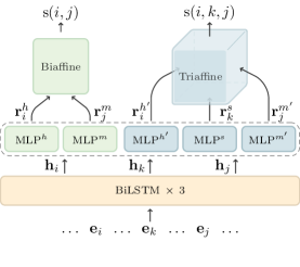
Figure 2: Scoring architecture with second-order extension.

Local token-wise training loss.

The biaffine parser adopts a simple non-structural training loss, trying to independently maximize the local probability of the correct head word for each word. For a gold-standard head-modifier pair ($w_{i}$, $w_{j}$) in a training instance, the cross-entropy loss is

$$\mathit{L}(i,j)=-\log{\frac{e^{s(i,j)}}{\sum_{0\leq k\leq n}e^{s(k,j)}}}$$ (4)

In other words, the model is trained based on simple head selection, without considering the tree structure at all, and losses of all words in a mini-batch are accumulated.

Decoding.

Having scores of all dependencies, we adopt the first-order Eisner algorithm with time complexity of $O(n^{3})$ to find the optimal tree.

$${\boldsymbol{y}}^{*}=\arg\max_{\boldsymbol{y}}\left[s(\boldsymbol{x},\boldsymbol{y})\equiv\sum_{i\rightarrow j\in\boldsymbol{y}}{s(i,j)}\right]$$ (5)

Handling dependency labels.

The biaffine parser treats skeletal tree searching and labeling as two independent (training phase) and cascaded (parsing phase) tasks. This work follows the same strategy for simplicity. Please refer to Dozat and Manning (2017) for details.

3 Second-order TreeCRF

This work substantially extends the biaffine parser in two closely related aspects: using probabilistic TreeCRF for structural training and explicitly incorporating high-order subtree scores. Specifically, we further incorporate adjacent-sibling subtree scores into the basic first-order model:

$$s(\boldsymbol{x},\boldsymbol{y})=\sum_{i\rightarrow j\in\boldsymbol{y}}s(i,j)+\sum_{i\rightarrow\{k,j\}\in\boldsymbol{y}}s(i,k,j)$$ (6)

where $k$ and $j$ are two adjacent modifiers of $i$ and satisfy either $i<k<j$ or $j<k<i$.

As a probabilistic model, TreeCRF computes the conditional probability of a tree as

$$\begin{split}&p(\boldsymbol{y}\mid\boldsymbol{x})=\frac{e^{s(\boldsymbol{x},\boldsymbol{y})}}{Z(\boldsymbol{x})\equiv\sum_{\boldsymbol{y^{\prime}}\in\mathcal{Y}(\boldsymbol{x})}{e^{s(\boldsymbol{x},\boldsymbol{y^{\prime}})}}}\end{split}$$ (7)

where $\mathcal{Y}(\boldsymbol{x})$ is the set of all legal (projective) trees for $\boldsymbol{x}$, and $Z(\boldsymbol{x})$ is commonly referred to as the normalization (or partition) term.

During training, TreeCRF employs the following structural training loss to maximize the conditional probability of the gold-standard tree $\boldsymbol{y}$ given $\boldsymbol{x}$.

$$\begin{split}\mathit{L}(\boldsymbol{x},\boldsymbol{y})&=-\log p(\boldsymbol{y}\mid\boldsymbol{x})\\ &=-s(\boldsymbol{x},\boldsymbol{y})+\log Z(\boldsymbol{x})\end{split}$$ (8)

Figure 3: Diagrams of the second-order inside algorithm based on bottom-up dynamic programming.

3.1 Scoring Second-order Subtrees

To avoid major modification to the original scoring architecture, we take a straightforward extension to obtain scores of adjacent-sibling subtrees. First, we employ three extra MLPs to perform similar feature extraction.

$$\mathbf{r}_{i}^{h^{\prime}};\mathbf{r}_{i}^{s};\mathbf{r}_{i}^{m^{\prime}}=\mathrm{MLP}^{h^{\prime}/s/m^{\prime}}\left(\mathbf{h}_{i}\right)$$ (9)

where $\mathbf{r}_{i}^{h^{\prime}};\mathbf{r}_{i}^{s};\mathbf{r}_{i}^{m^{\prime}}$ are the representation vectors of $w_{i}$ as head, sibling, and modifier respectively.

Then, we propose a natural extension to the biaffine equation, and employ triaffine for score computation over three vectors.

$$s(i,k,j)=\left[\begin{array}[]{c}\mathbf{r}_{k}^{s}\\ 1\end{array}\right]^{\mathrm{T}}{\mathbf{r}_{i}^{h^{\prime}}}^{\mathrm{T}}\mathbf{W}^{\textit{triaffine}}\left[\begin{array}[]{c}\mathbf{r}_{j}^{m^{\prime}}\\ 1\end{array}\right]$$ (10)

where $\mathbf{W}^{\textit{triaffine}}\in\mathbb{R}^{d^{\prime}\times d^{\prime}\times d^{\prime}}$ is a three-way tensor. The triaffine computation can be quite efficiently performed with the $\mathrm{einsum}$ function on PyTorch.

3.2 Computing TreeCRF Loss Efficiently

The key to TreeCRF loss is how to efficiently compute $\log Z(\boldsymbol{x})$, as shown in Equation 8. This problem has been well solved long before the DL era for non-neural dependency parsing. Straightforwardly, we can directly extend the viterbi decoding algorithm by replacing max product with sum product, and naturally obtain $\log Z(\boldsymbol{x})$ in the same polynomial time complexity. However, it is not enough to solely perform the inside algorithm for non-neural parsing, due to the inapplicability of the automatic differentiation mechanism. In order to obtain marginal probabilities and then feature weight gradients, we have to realize the more sophisticated outside algorithm, which is usually at least twice slower than the inside algorithm. This may be the major reason for the less popularity of TreeCRF (vs. max-margin training) before the DL era.

1:  define: $I,S,C\in\mathbb{R}^{n\times n\times B}$ $\rhd$ $B$ is #sents in a batch

2:  initialize: $C_{i,i}=\log e^{0}=0,0\leq i\leq n$

3:  for $w=1$ to $n$ do $\rhd$ span width

4:     Batchify: $0\leq i$; $j=i+w\leq n$

5:     $I_{i,j}=\log\left(\begin{array}[]{l}e^{C_{i,i}+C_{j,i+1}}~{}+\\ \sum\limits_{i<r<j}e^{I_{i,r}+S_{r,j}+s(i,r,j)}\\ \end{array}\right)$ + s(i, j)

6:     $S_{i,j}=\log\sum\limits_{i\leq r<j}e^{C_{i,r}+C_{j,r+1}}$

7:     $C_{i,j}=\log\sum\limits_{i<r\leq j}e^{I_{i,r}+C_{r,j}}$

8:  end for$\rhd$ refer to Figure 3

9:  return  $C_{0,n}\equiv\log Z$

Algorithm 1 Second-order Inside Algorithm.

As far as we know, all previous works on neural TreeCRF parsing explicitly implement the inside-outside algorithm for gradient computation Zhang et al. (2019); Jiang et al. (2018). To improve efficiency, computation is transferred from GPUs to CPUs with Cython programming.

This work shows that the inside algorithm can be effectively batchified to fully utilize the power of GPUs. Figure 3 and Algorithm 1 together illustrate the batchified version of the second-order inside algorithm, which is a direct extension of the second-order Eisner algorithm in McDonald and Pereira (2006) by replacing max product with sum product. We omit the generations of incomplete, complete, and sibling spans in the opposite direction from $j$ to $i$ for brevity.

Basically, we first pack the scores of same-width spans at different positions ($i,j$) for all $B$ sentences in the data batch into large tensors. Then we can do computation and aggregation simultaneously on GPUs via efficient large tensor operation.

Similarly, we also batchify the decoding algorithm. Due to space limitation, we omit the details.

It is noteworthy that the techniques described here are also applicable to other grammar formulations such as CKY-style constituency parsing Finkel et al. (2008); Drozdov et al. (2019).

3.3 Outside via Back-propagation

Eisner (2016) proposes a theoretical proof on the equivalence between the back-propagation mechanism and the outside algorithm in the case of constituency (phrase-structure) parsing. This work empirically verifies this equivalence for dependency parsing.

Moreover, we also find that marginal probabilities $p(i\rightarrow j\mid\boldsymbol{x})$ directly correspond to gradients after back-propagation with $\log Z(\boldsymbol{x})$ as the loss:

$$\begin{split}\frac{\partial\log Z}{\partial\mathrm{s}(i,j)}&=\sum_{\boldsymbol{y}:(i,j)\in\boldsymbol{{y}}}p(\boldsymbol{y}\mid\boldsymbol{x})=p(i\rightarrow j\mid\boldsymbol{x})\end{split}$$ (11)

which can be easily proved. For TreeCRF parsers, we perform MBR decoding Smith and Smith (2007) by replacing scores with marginal probabilities in the decoding algorithm, leading to a slight but consistent accuracy increase.

3.4 Handling Partial Annotation

As an attractive research direction, studies show that it is more effective to construct or even collect partially labeled data Nivre et al. (2014); Hwa (1999); Pereira and Schabes (1992), where a sentence may correspond to a partial tree $|{\boldsymbol{y}^{p}}|<n$ in the case of dependency parsing. Partial annotation can be very powerful when combined with active learning, because annotation cost can be greatly reduced if annotators only need to annotate sub-structures that are difficult for models. Li et al. (2016) present a detailed survey on this topic. Moreover, Peng et al. (2019) recently released a partially labeled multi-domain Chinese dependency treebank based on this idea.

Then, the question is how to train models on partially labeled data. Li et al. (2016) propose to extend TreeCRF for this purpose and obtain promising results in the case of non-neural dependency parsing. This work applies their approach to the neural biaffine parser. We are particularly concerned at the influence of structural learning and high-order modeling on the utilization of partially labeled training data.

For the basic biaffine parser based on first-order local training, it seems the only choice is omitting losses of unannotated words. In contrast, tree constraints allow annotated dependencies to influence the probability distributions of unannotated words, and high-order modeling further helps by promoting inter-token interaction. Therefore, both structural learning and high-order modeling are intuitively very beneficial.

Under partial annotation, we follow Li et al. (2016) and define the training loss as:

$$\begin{split}\mathit{L}(\boldsymbol{x},{\boldsymbol{y}^{p}})&=-\log\sum\limits_{\boldsymbol{y}\in\mathcal{Y}(\boldsymbol{x});\boldsymbol{y}\supseteq{\boldsymbol{y}^{p}}}p(\boldsymbol{y}\mid\boldsymbol{x})\\ &=-\log\frac{Z(\boldsymbol{x},{\boldsymbol{y}^{p}})\equiv\sum\limits_{\boldsymbol{y}\in\mathcal{Y}(\boldsymbol{x});\boldsymbol{y}\supseteq\boldsymbol{y}^{p}}e^{s(\boldsymbol{x},\boldsymbol{y})}}{Z(\boldsymbol{x})}\end{split}$$ (12)

where $Z(\boldsymbol{x},{\boldsymbol{y}^{p}})$ only considers all legal trees that are compatible with the given partial tree and can also be efficiently computed like $Z(\boldsymbol{x})$.

4 Experiments

Data.

We conduct experiments and analysis on 27 datasets from 13 languages, including two widely used datasets: the English Penn Treebank (PTB) data with Stanford dependencies Chen and Manning (2014), and the Chinese data at the CoNLL09 shared task Hajič et al. (2009).

We also adopt the Chinese dataset released at the NLPCC19 cross-domain dependency parsing shared task Peng et al. (2019), containing one source domain and three target domains. For simplicity, we directly merge the train/dev/test data of the four domains into larger ones respectively. One characteristic of the data is that most sentences are partially annotated based on active learning.

Finally, we conduct experiments on Universal Dependencies (UD) v2.2 and v2.3 following Ji et al. (2019) and Zhang et al. (2019) respectively. We adopt the 300d multilingual pretrained word embeddings used in Zeman et al. (2018) and take the CharLSTM representations as input. For UD2.2, to compare with Ji et al. (2019), we follow the raw text setting of the CoNLL18 shared task Zeman et al. (2018), and directly use their sentence segmentation and tokenization results. For UD2.3, we also report the results of using gold-standard POS tags to compare with Zhang et al. (2019).

Evaluation metrics.

We use unlabeled and labeled attachment score (UAS/LAS) as the main metrics. Punctuations are omitted for PTB. For the partially labeled NLPCC19 data, we adopt the official evaluation script, which simply omits the words without gold-standard heads to accommodate partial annotation. We adopt Dan Bikel’s randomized parsing evaluation comparator for significance test.

Parameter settings.

We directly adopt most parameter settings of Dozat and Manning (2017), including dropout and initialization strategies. For CharLSTM, the dimension of input char embeddings is 50, and the dimension of output vector is 100, following Lample et al. (2016). For the second-order model, we set the dimensions of $\mathbf{r}^{h^{\prime}/s/m^{\prime}}_{i}$ to 100, and find little accuracy improvement when increasing to 300. We trained each model for at most 1,000 iterations, and stop training if the peak performance on the dev data does not increase in 100 consecutive epochs.

Models.

Loc uses local cross-entropy training loss and employs the Eisner algorithm for finding the optimal projective tree. Crf and Crf2o denote the first-order and second-order TreeCRF model respectively. $\textsc{Loc}_{\textsc{mst}}$ denotes the basic local model that directly produces non-projective tree based on the MST decoding algorithm of Dozat and Manning (2017).

4.1 Efficiency Comparison

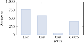
Figure 4: Parsing speed comparison on PTB-test.

Figure 4 compares the parsing speed of different models on PTB-test. For a fair comparison, we run all models on the same machine with Intel Xeon CPU (E5-2650v4, 2.20GHz) and GeForce GTX 1080 Ti GPU. “Crf (cpu)” refers to the model that explicitly performs the inside-outside algorithm using Cython on CPUs. Multi-threading is employed since sentences are mutually independent. However, we find that using more than 4 threads does not further improve the speed.

We can see that the efficiency of TreeCRF is greatly improved by batchifying the inside algorithm and implicitly realizing the outside algorithm by back-propagation on GPUs. For the first-order Crf model, our implementation can parse about 500 sentences per second, over 10 times faster than the multi-thread “Crf (cpu)”. For the second-order Crf2o, our parser achieves the speed of 400 sentences per second, which is able to meet the requirements of a real-time system. More discussions on efficiency are presented in Appendix A.

	Dev		Test
	UAS	LAS	UAS	LAS
PTB
Biaffine17	-	-	95.74	94.08
F&K19	-	-	-	91.59
Li19	95.76	93.97	95.93	94.19
Ji19	95.88	93.94	95.97	94.31
Zhang19	-	-	-	93.96
Loc	95.82	93.99	96.08	94.47
Crf w/o MBR	95.74	93.96	96.04	94.34
Crf	95.76	93.99	96.02	94.33
Crf2o w/o MBR	95.92	94.16	96.14	94.49
Crf2o	95.90	94.12	96.11	94.46
CoNLL09
Biaffine17	-	-	88.90	85.38
Li19	88.68	85.47	88.77	85.58
Loc	89.07	86.10	89.15	85.98
Crf w/o MBR	89.04	86.04	89.14	86.06
Crf	89.12	86.12	89.28	86.18†
Crf2o w/o MBR	89.29	86.24	89.49	86.39
Crf2o	89.44	86.37	89.63‡	86.52‡
NLPCC19
Loc	77.01	71.14	76.92	71.04
Crf w/o MBR	77.40	71.65	77.17	71.58
Crf	77.34	71.62	77.53‡	71.89‡
Crf2o w/o MBR	77.58	71.92	77.89	72.25
Crf2o	78.08	72.32	78.02‡	72.33‡

Table 1: Main results. We perform significance test against Loc on the test data, where “$\dagger$” means $\mathrm{p}<0.05$ and “$\ddagger$” means $\mathrm{p}<0.005$. Biaffine17: Dozat and Manning (2017); F&K19: Falenska and Kuhn (2019); Li19: Li et al. (2019); Ji19: Ji et al. (2019); Zhang19: Zhang et al. (2019).

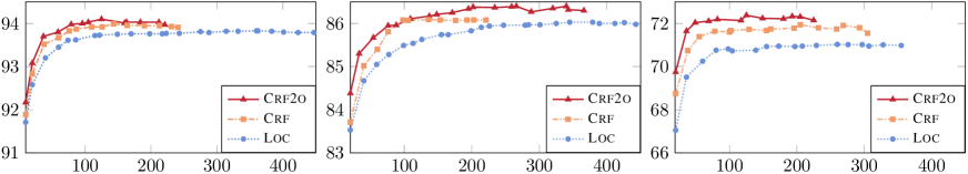
Figure 5: Convergence curves (LAS vs. training epochs) on dev data of PTB, CoNLL09, and NLPCC19.

4.2 Main Results

Table 1 lists the main results on the dev and test data. The trends on dev and test are mostly consistent. For a fair comparison with previous works, we only consider those without using extra resources such as ELMo Peters et al. (2018) and BERT Devlin et al. (2019). We can see that our baseline Loc achieves the best performance on both PTB and CoNLL09.

On PTB, both Crf and Crf2o fail to improve the parsing accuracy further, probably because the performance is already very high. However, as shown by further analysis in Section 4.3, the positive effect is actually introduced by structural learning and high-order modeling.

On CoNLL09, Crf significantly outperforms Loc, and Crf2o can further improve the performance.

On the partially annotated NLPCC19 data, Crf outperforms Loc by a very large margin, indicating the usefulness of structural learning in the scenario of partial annotation. Crf2o further improves the parsing performance by explicitly modeling second-order subtree features. These results confirm our intuitions discussed in Section 3.4. Please note that the parsing accuracy looks very low because the partially annotated tokens are usually difficult for models.

4.3 Analysis

	SIB			UCM	LCM
	P	R	F
PTB
Loc	91.16	90.80	90.98	61.59	50.66
Crf	91.24	90.92	91.08	61.92	50.33
Crf2o	91.56	91.11	91.33	63.08	50.99
CoNLL09
Loc	79.20	79.02	79.11	40.10	28.91
Crf	79.17	79.55	79.36	40.61	29.38
Crf2o	81.00	80.63	80.82	42.53	30.09

Table 2: Sub- and full-tree performance on test data.

Impact of MBR decoding.

For Crf and Crf2o, we by default to perform MBR decoding, which employs the Eisner algorithm over marginal probabilities Smith and Smith (2007) to find the best tree.

$$\begin{split}&{\boldsymbol{y}}^{*}=\arg\max_{\boldsymbol{y}}\left[\sum_{i\rightarrow j\in\boldsymbol{y}}{p(i\rightarrow j|\boldsymbol{x})}\right]\end{split}$$ (13)

Table 1 reports the results of directly finding 1-best trees according to dependency scores. Except for PTB, probably due to the high accuracy already, MBR decoding brings small yet consistent improvements for both Crf and Crf2o.

Convergence behavior.

Figure 5 compares the convergence curves. For clarity, we plot one data point corresponding to the peak LAS every 20 epochs. We can clearly see that both structural learning and high-order modeling consistently improve the model. Crf2o achieves steadily higher accuracy and converges much faster than the basic Loc.

Performance at sub- and full-tree levels.

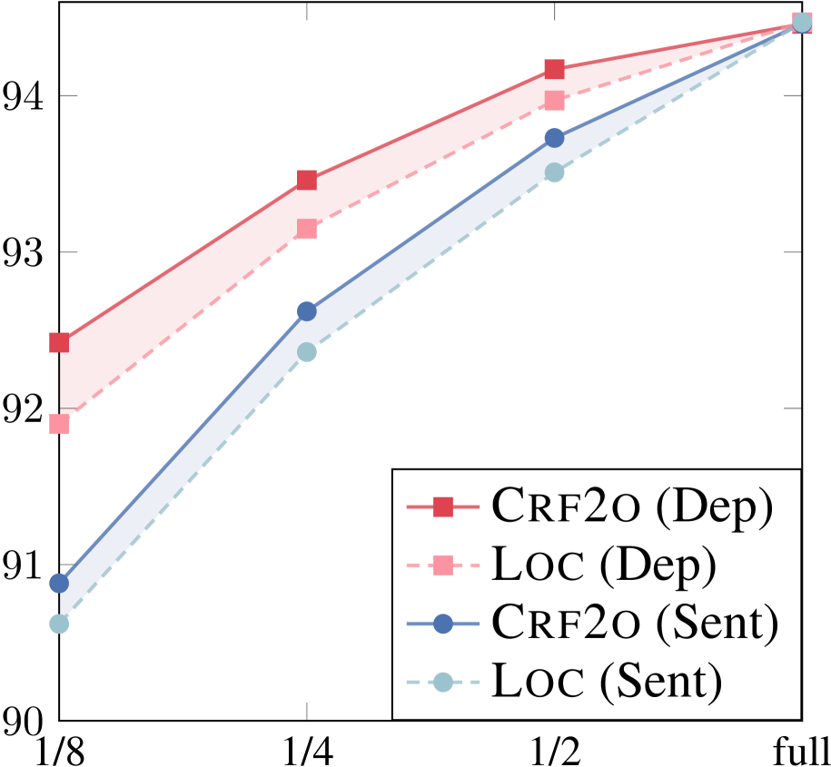
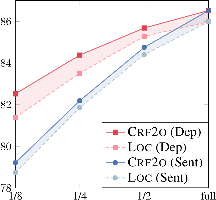
Figure 6: LAS on PTB (left) and CoNLL09-test (right) regarding the amount of training data (dependencies vs. sentences).

	bg	ca	cs	de	en	es	fr	it	nl	no	ro	ru	Avg.
UD2.2
$\textsc{Loc}_{\textsc{mst}}$	90.44	91.11	91.04	80.21	86.86	90.67	87.99	91.19	88.24	90.35	86.24	93.01	88.95
Loc	90.45	91.14	90.97	80.02	86.83	90.56	87.76	91.14	87.72	90.74	86.20	93.01	88.88
Crf	90.73	91.25	91.01	80.56†	86.92	90.81†	88.16	91.64†	88.10	90.85	86.50	93.17†	89.14‡
Crf2o	90.77	91.29	91.54†	80.46	87.32†	90.86†	87.96	91.91‡	88.62‡	91.02†	86.90‡	93.33‡	89.33‡
using raw text
Ji19	88.28	89.90	89.85	77.09	81.16	88.93	83.73	88.91	84.82	86.33	84.44	86.62	85.83
Crf2o	89.72	91.27	90.94	78.26	82.88	90.79	86.33	91.02	87.92	90.17	85.71	92.49	88.13
UD2.3
$\textsc{Loc}_{\textsc{mst}}$	90.56	91.03	91.98	81.59	86.83	90.64	88.23	91.67	88.20	90.63	86.51	93.03	89.23
Loc	90.57	91.10	91.85	81.68	86.54	90.47	88.40	91.53	88.18	90.65	86.31	92.91	89.19
Crf	90.52	91.19	92.02	81.43	86.88†	90.76†	88.75	91.76	88.08	90.79	86.54	93.16‡	89.32‡
Crf2o	90.76	91.12	92.15‡	81.94	86.93†	90.81‡	88.83†	92.34‡	88.21†	90.78	86.62	93.22‡	89.48‡
using gold POS tags
Zhang19	90.15	91.39	91.10	83.39	88.52	90.84	88.59	92.49	88.37	92.82	84.89	93.11	89.85
Crf2o	91.32	92.57	92.66	84.56	88.98	91.88	89.83	92.94	89.85	93.26	87.39	93.86	90.76

Table 3: LAS on UD2.2 and UD2.3 test datasets. Again, $\dagger$ and $\ddagger$ means significance level at $p<0.05$ and $p<0.005$ respectively against the Loc parser.

Beyond the dependency-wise accuracy (UAS/LAS), we would like to evaluate the models regarding performance at sub-tree and full-tree levels. Table 2 shows the results. We skip the partially labeled NLPCC19 data. UCM means unlabeled complete matching rate, i.e., the percent of sentences obtaining whole correct skeletal trees, while LCM further requires that all labels are also correct.

For SIB, we evaluate the model regarding unlabeled adjacent-sibling subtrees (system outputs vs. gold-standard references). According to Equation 6, $(i,k,j)$ is an adjacent-sibling subtree, if and only if $w_{k}$ and $w_{j}$ are both children of $w_{i}$ at the same side, and there are no other children of $w_{i}$ between them. Given two trees, we can collect all adjacent-sibling subtrees and compose two sets of triples. Then we evaluate the P/R/F values. Please note that it is impossible to evaluate SIB for partially annotated references.

We can clearly see that by modeling adjacent-sibling subtree scores, the SIB performance obtains larger improvement than both Crf and Loc, and this further contributes to the large improvement on full-tree matching rates (UCM/LCM).

Capability to learn from partial trees.

To better understand why Crf2o performs very well on partially annotated NLPCC19, we design more comparative experiments by retaining either a proportion of random training sentences (full trees) or a proportion of random dependencies for each sentence (partial trees). Figure 6 shows the results.

We can see that the performance gap is quite steady when we gradually reduce the number of training sentences. In contrast, the gap clearly becomes larger when each training sentence has less annotated dependencies. This shows that Crf2o is superior to the basic Loc in utilizing partial annotated data for model training.

4.4 Results on Universal Dependencies

Table 3 compares different models on UD datasets, which contain a lot of non-projective trees. We adopt the pseudo-projective approach Nivre and Nilsson (2005) for handling the ubiquitous non-projective trees of most languages. Basically, the idea is to transform non-projective trees into projective ones using more complex labels for post-processing recovery.

We can see that for the basic local parsers, the direct non-projective $\textsc{Loc}_{\textsc{mst}}$ and the pseudo-projective Loc achieve very similar performance.

More importantly, both Crf and Crf2o produce consistent improvements over the baseline in many languages. On both UD2.2 and UD2.3, Our proposed Crf2o model achieves the highest accuracy for 10 languages among 12, and obtains significant improvement in more than 7 languages. Overall, the averaged improvement is 0.45 and 0.29 on UD2.2 and UD2.3 respectively, which is also significant at $p<0.005$.

On average, our Crf2o parser outperforms Ji et al. (2019) by 2.30 on UD2.2 raw texts following CoNLL-2018 shared task setting, and Zhang et al. (2019) by 0.91 on UD2.3 data with gold POS tags. It is noteworthy that the German (de) result is kindly provided by Tao Ji after rerunning their parser with predicted XPOS tags, since their reported result in Ji et al. (2019) accidentally used gold-standard sentence segmentation, tokenization, and XPOS tags. Our Crf2o parser achieves an average LAS of 87.64 using their XPOS tags.

5 Related Works

Batchification has been widely used in linear-chain CRF, but is rather complicated for tree structures. Eisner (2016) presents a theoretical proof on the equivalence of outside and back-propagation for constituent tree parsing, and also briefly discusses other formalisms such as dependency grammar. Unfortunately, we were unaware of Eisner’s great work until we were surveying the literature for paper writing. As an empirical study, we believe this work is valuable and makes it practical to deploy TreeCRF models in real-life systems.

Falenska and Kuhn (2019) present a nice analytical work on dependency parsing, similar to Gaddy et al. (2018) on constituency parsing. By extending the first-order graph-based parser of Kiperwasser and Goldberg (2016) into second-order, they try to find out how much structural context is implicitly captured by the BiLSTM encoder. They concatenate three BiLSTM output vectors ($i,k,j$) for scoring adjacent-sibling subtrees, and adopt max-margin loss and the second-order Eisner decoding algorithm McDonald and Pereira (2006). Based on their negative results and analysis, they draw the conclusion that high-order modeling is redundant because BiLSTM can implicitly and effectively encode enough structural context. They also present a nice survey on the relationship between RNNs and syntax. In this work, we use a much stronger basic parser and observe more significant UAS/LAS improvement than theirs. Particularly, we present an in-depth analysis showing that explicitly high-order modeling certainly helps the parsing model and thus is complementary to the BiLSTM encoder.

Ji et al. (2019) employ graph neural networks to incorporate high-order structural information into the biaffine parser implicitly. They add a three-layer graph attention network (GAT) component Veličković et al. (2018) between the MLP and Biaffine layers. The first GAT layer takes $\mathbf{r}_{i}^{h}$ and $\mathbf{r}_{i}^{m}$ from MLPs as inputs and produces new representation $\mathbf{r}_{i}^{h1}$ and $\mathbf{r}_{i}^{m1}$ by aggregating neighboring nodes. Similarly, the second GAT layer operates on $\mathbf{r}_{i}^{h1}$ and $\mathbf{r}_{i}^{m1}$, and produces $\mathbf{r}_{i}^{h2}$ and $\mathbf{r}_{i}^{m2}$. In this way, a node gradually collects multi-hop high-order information as global evidence for scoring single dependencies. They follow the original local head-selection training loss. In contrast, this work adopts global TreeCRF loss and explicitly incorporates high-order scores into the biaffine parser.

Zhang et al. (2019) investigate the usefulness of structural training for the first-order biaffine parser. They compare the performance of local head-selection loss, global max-margin loss, and TreeCRF loss on multilingual datasets. They show that TreeCRF loss is overall slightly superior to max-margin loss, and LAS improvement from structural learning is modest but significant for some languages. They also show that structural learning (especially TreeCRF) substantially improves sentence-level complete matching rate, which is consistent with our findings. Moreover, they explicitly compute the inside and outside algorithms on CPUs via Cython programming. In contrast, this work proposes an efficient second-order TreeCRF extension to the biaffine parser, and presents much more in-depth analysis to show the effect of both structural learning and high-order modeling.

6 Conclusions

This paper for the first time presents second-order TreeCRF for neural dependency parsing using triaffine for explicitly scoring second-order subtrees. We propose to batchify the inside algorithm to accommodate GPUs. We also empirically verify that the complex outside algorithm can be implicitly performed via efficient back-propagation, which naturally produces gradients and marginal probabilities. We conduct experiments and detailed analysis on 27 datasets from 13 languages, and find that structural learning and high-order modeling can further enhance the state-of-the-art biaffine parser in various aspects: 1) better convergence behavior; 2) higher performance on sub- and full-tree levels; 3) better utilization of partially annotated data.

Appendix A More on Efficiency

Training speed.

During training, we greedily find the 1-best head for each word without tree constraints. Therefore, the processing speed is faster than the evaluation phase. Specifically, for Loc, Crf and Crf2o, the average one-iteration training time is about 1min, 2.5min and 3.5min on PTB. In other words, the parser consumes about 700/300/200 sentences per second.

MST decoding.

As Dozat et al. (2017) pointed out, they adopted an ad-hoc approximate algorithm which does not guarantee to produce the highest-scoring tree, rather than the ChuLiu/Edmonds algorithm for MST decoding. The time complexity of the ChuLiu/Edmonds algorithm is $O(n^{2})$ under the optimized implementation of Tarjan (1977). Please see the discussion of McDonald et al. (2005b) for details.

For $\textsc{Loc}_{\textsc{mst}}$, we directly borrow the MST decoding approach in the original parser of Dozat and Manning (2017). $\textsc{Loc}_{\textsc{mst}}$ achieves 94.43 LAS on PTB-test (inferior to 94.47 of Loc, see Table 1), and its parsing speed is over 1000 sentences per second.

Faster decoding strategy.

Inspired by the idea of ChuLiu/Edmonds algorithm, we can further improve the efficiency of the CRF parsing models by avoiding the Eisner decoding for some sentences. The idea is that if by greedily assigning a local max-scoring head word to each word, we can already obtain a legal projective tree, then we omit the decoding process for the sentence. We can judge whether an output is a legal tree (single root and no cycles) using the Tarjan algorithm in $O(n)$ time complexity. Further, we can judge whether a tree is a projective tree also in a straightforward way very efficiently. In fact, we find that more than 99% sentences directly obtain legal projective trees on PTB-test by such greedy assignment on marginal probabilities first. We only need to run the decoding algorithm for the left sentences.

References

- Cai et al. (2017) Jiong Cai, Yong Jiang, and Kewei Tu. 2017. CRF autoencoder for unsupervised dependency parsing. In Proceedings of EMNLP, pages 1638–1643.
- Carreras (2007) Xavier Carreras. 2007. Experiments with a higher-order projective dependency parser. In Proceedings of EMNLP, pages 957–961.
- Chen and Manning (2014) Danqi Chen and Christopher Manning. 2014. A fast and accurate dependency parser using neural networks. In Proceedings of EMNLP, pages 740–750.
- Devlin et al. (2019) Jacob Devlin, Ming-Wei Chang, Kenton Lee, and Kristina Toutanova. 2019. BERT: Pre-training of deep bidirectional transformers for language understanding. In Proceedings of NAACL, pages 4171–4186.
- Dozat and Manning (2017) Timothy Dozat and Christopher D. Manning. 2017. Deep biaffine attention for neural dependency parsing. In Proceedings of ICLR.
- Dozat et al. (2017) Timothy Dozat, Peng Qi, and Christopher D. Manning. 2017. Stanford’s graph-based neural dependency parser at the CoNLL 2017 shared task. In Proceedings of CoNLL, pages 20–30.
- Drozdov et al. (2019) Andrew Drozdov, Patrick Verga, Mohit Yadav, Mohit Iyyer, and Andrew McCallum. 2019. Unsupervised latent tree induction with deep inside-outside recursive auto-encoders. In Proceedings of NAACL, pages 1129–1141.
- Eisner (2000) Jason Eisner. 2000. Bilexical grammars and their cubic-time parsing algorithms. In Advances in Probabilistic and Other Parsing Technologies.
- Eisner (2016) Jason Eisner. 2016. Inside-outside and forward-backward algorithms are just backprop (tutorial paper). In Proceedings of WS, pages 1–17.
- Falenska and Kuhn (2019) Agnieszka Falenska and Jonas Kuhn. 2019. The (non-)utility of structural features in BiLSTM-based dependency parsers. In Proceedings of ACL, pages 117–128.
- Finkel et al. (2008) Jenny Rose Finkel, Alex Kleeman, and Christopher D. Manning. 2008. Efficient, feature-based, conditional random field parsing. In Proceedings of ACL, pages 959–967.
- Gaddy et al. (2018) David Gaddy, Mitchell Stern, and Dan Klein. 2018. What’s going on in neural constituency parsers? an analysis. In Proceedings of NAACL, pages 999–1010.
- Hajič et al. (2009) Jan Hajič, Massimiliano Ciaramita, Richard Johansson, Daisuke Kawahara, Maria Antònia Martí, Lluís Màrquez, Adam Meyers, Joakim Nivre, Sebastian Padó, Jan Štěpánek, Pavel Straňák, Mihai Surdeanu, Nianwen Xue, and Yi Zhang. 2009. The CoNLL-2009 shared task: Syntactic and semantic dependencies in multiple languages. In Proceedings of CoNLL, pages 1–18.
- Hwa (1999) Rebecca Hwa. 1999. Supervised grammar induction using training data with limited constituent information. In Proceedings of ACL, pages 73–79.
- Ji et al. (2019) Tao Ji, Yuanbin Wu, and Man Lan. 2019. Graph-based dependency parsing with graph neural networks. In Proceedings of ACL, pages 2475–2485.
- Jiang et al. (2018) Xinzhou Jiang, Zhenghua Li, Bo Zhang, Min Zhang, Sheng Li, and Luo Si. 2018. Supervised treebank conversion: Data and approaches. In Proceedings of ACL, pages 2706–2716.
- Kiperwasser and Goldberg (2016) Eliyahu Kiperwasser and Yoav Goldberg. 2016. Simple and accurate dependency parsing using bidirectional LSTM feature representations. Transactions of ACL, pages 313–327.
- Koo and Collins (2010) Terry Koo and Michael Collins. 2010. Efficient third-order dependency parsers. In Proceedings of ACL, pages 1–11.
- Lample et al. (2016) Guillaume Lample, Miguel Ballesteros, Sandeep Subramanian, Kazuya Kawakami, and Chris Dyer. 2016. Neural architectures for named entity recognition. In Proceedings of NAACL, pages 2475–2485.
- Le and Zuidema (2014) Phong Le and Willem Zuidema. 2014. The inside-outside recursive neural network model for dependency parsing. In Proceedings of EMNLP, pages 729–739.
- Li et al. (2019) Ying Li, Zhenghua Li, Min Zhang, Rui Wang, Sheng Li, and Luo Si. 2019. Self-attentive biaffine dependency parsing. In Proceedings of IJCAI, pages 5067–5073.
- Li et al. (2016) Zhenghua Li, Min Zhang, Yue Zhang, Zhanyi Liu, Wenliang Chen, Hua Wu, and Haifeng Wang. 2016. Active learning for dependency parsing with partial annotation. In Proceedings of ACL, pages 344–354.
- Ma and Zhao (2012) Xuezhe Ma and Hai Zhao. 2012. Fourth-order dependency parsing. In Proceedings of COLING, pages 785–796.
- McDonald et al. (2005a) Ryan McDonald, Koby Crammer, and Fernando Pereira. 2005a. Online large-margin training of dependency parsers. In Proceedings of ACL, pages 91–98.
- McDonald and Pereira (2006) Ryan McDonald and Fernando Pereira. 2006. Online learning of approximate dependency parsing algorithms. In Proceedings of EACL, pages 81–88.
- McDonald et al. (2005b) Ryan McDonald, Fernando Pereira, Kiril Ribarov, and Jan Hajič. 2005b. Non-projective dependency parsing using spanning tree algorithms. In Proceedings of EMNLP, pages 523–530.
- Nivre et al. (2014) Joakim Nivre, Yoav Goldberg, and Ryan McDonald. 2014. Squibs: Constrained arc-eager dependency parsing. CL, pages 249–257.
- Nivre et al. (2016) Joakim Nivre, Marie-Catherine de Marneffe, Filip Ginter, Yoav Goldberg, Jan Hajic, Christopher D. Manning, Ryan McDonald, Slav Petrov, Sampo Pyysalo, Natalia Silveira, Reut Tsarfaty, and Daniel Zeman. 2016. Universal dependencies v1: A multilingual treebank collection. In Proceedings of LREC, pages 1659–1666.
- Nivre and Nilsson (2005) Joakim Nivre and Jens Nilsson. 2005. Pseudo-projective dependency parsing. In Proceedings of ACL, pages 99–106.
- Pei et al. (2015) Wenzhe Pei, Tao Ge, and Baobao Chang. 2015. An effective neural network model for graph-based dependency parsing. In Proceedings of ACL-IJCNLP, pages 313–322.
- Peng et al. (2019) Xue Peng, Zhenghua Li, Min Zhang, Rui Wang, Yue Zhang, and Luo Si. 2019. Overview of the nlpcc 2019 shared task: cross-domain dependency parsing. In Proceedings of NLPCC, pages 760–771.
- Pereira and Schabes (1992) Fernando Pereira and Yves Schabes. 1992. Inside-outside reestimation from partially bracketed corpora. In Proceedings of ACL, pages 128–135.
- Peters et al. (2018) Matthew Peters, Mark Neumann, Mohit Iyyer, Matt Gardner, Christopher Clark, Kenton Lee, and Luke Zettlemoyer. 2018. Deep contextualized word representations. In Proceedings of NAACL, pages 2227–2237.
- Smith and Smith (2007) David A. Smith and Noah A. Smith. 2007. Probabilistic models of nonprojective dependency trees. In Proceedings of EMNLP, pages 132–140.
- Tarjan (1977) Robert Endre Tarjan. 1977. Finding optimum branchings. Networks, pages 25–35.
- Veličković et al. (2018) Petar Veličković, Guillem Cucurull, Arantxa Casanova, Adriana Romero, Pietro Liò, and Yoshua Bengio. 2018. Graph attention networks. In Proceedings of ICLR.
- Wang and Chang (2016) Wenhui Wang and Baobao Chang. 2016. Graph-based dependency parsing with bidirectional LSTM. In Proceedings of ACL, pages 2475–2485.
- Wang et al. (2019) Xinyu Wang, Jingxian Huang, and Kewei Tu. 2019. Second-order semantic dependency parsing with end-to-end neural networks. In Proceedings of ACL, pages 4609–4618.
- Zeman et al. (2018) Daniel Zeman, Jan Hajič, Martin Popel, Martin Potthast, Milan Straka, Filip Ginter, Joakim Nivre, and Slav Petrov. 2018. CoNLL 2018 shared task: Multilingual parsing from raw text to universal dependencies. In Proceedings of CoNLL, pages 1–21.
- Zhang et al. (2017) Xingxing Zhang, Jianpeng Cheng, and Mirella Lapata. 2017. Dependency parsing as head selection. In Proceedings of EACL, pages 665–676.
- Zhang et al. (2019) Zhisong Zhang, Xuezhe Ma, and Eduard Hovy. 2019. An empirical investigation of structured output modeling for graph-based neural dependency parsing. In Proceedings of ACL, pages 5592–5598.