Optimization in First-Passage Resetting

Abstract

We investigate classic diffusion with the added feature that a diffusing particle is reset to its starting point each time the particle reaches a specified threshold. In an infinite domain, this process is non-stationary and its probability distribution exhibits rich features. In a finite domain, we define a non-trivial optimization in which a cost is incurred whenever the particle is reset and a reward is obtained while the particle stays near the reset point. We derive the condition to optimize the net gain in this system, namely, the reward minus the cost.

Diffusion is a fundamental process underlying a wide variety of stochastic phenomena that has broad applications to physics, chemistry, finance, and social sciences Chandrasekhar (1943); Van Kampen (1992); Chicheportiche and Bouchaud (2014); Rogers (2010). A fruitful recent development is the notion of resetting, in which a diffusing particle is reset to its starting point at a specified rate Evans and Majumdar (2011a, b); Evans et al. (2020). Resetting alters the diffusive motion in fundamental ways and has sparked much research on its rich consequences (see, e.g., Boyer and Solis-Salas (2014); Christou and Schadschneider (2015); Rotbart et al. (2015); Majumdar et al. (2015); Reuveni (2016); Pal and Reuveni (2017); Belan (2018); Bodrova et al. (2019)). Resetting also has natural applications to search processes, where the search begins anew if the target is not found within a certain time Kuśmierz and Gudowska-Nowak (2015); Campos and Méndez (2015); Bhat et al. (2016); Eule and Metzger (2016). For such diffusive searches, resetting leads to a dramatic effect: an infinite search time to find a target becomes finite, with the search time minimized at a critical reset rate.

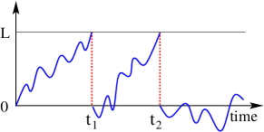
Figure 1: First-passage resetting on the semi-infinite line. Whenever a diffusing particle, which starts at the origin, reaches $L$, it is instantaneously reset to the origin. Successive first-passage times are denoted by $t_{1},t_{2},\ldots$.

In this work, we investigate first-passage resetting in which resetting occurs whenever a diffusing particle reaches a threshold location (Fig. 1). Hence the time of the reset event is determined by the state of the system itself rather than being imposed externally Evans and Majumdar (2011a, b); Evans et al. (2020). First-passage resetting typifies regenerative processes that are reset at renewals Ross (2014), which has natural applications to reliability theory Gnedenko et al. (2014). This mechanism was first envisaged by Feller Feller (1954) who proved existence and uniqueness theorems. Similar ideas were pursued in Sherman (1958), and they first appear in the physics literature in Falcao and Evans (2017). Specifically, Falcao and Evans (2017) examines two Brownian particles biased toward each other that reset to their initial positions upon encounter. This corresponds to a drift toward the origin in our semi-infinite geometry of Fig. 1. This negative drift leads to a stationary state, but the absence of drift leads to a variety of new phenomena, as discussed below. Moreover, we introduce a path decomposition that provides the spatial probability distribution in a geometric way.

When the diffusing particle is confined to the finite interval $[0,L]$, we define an optimization problem in which there is a cost for each resetting event and an increasing reward as the particle approaches the resetting point $x=L$. This scenario is inspired by a power-management problem Ajjarapu et al. (1994); Zhihong Feng et al. (2000), where the power delivered corresponds to the coordinate $x$ and a blackout corresponds to resetting. A closely related optimization arises in finance Miller and Orr (1966). In both examples, one seeks to operate almost to full capacity while avoiding saturation: in our optimization framework, the goal is to maximize the net gain—the difference between the reward and the cost.

Semi-Infinite Geometry: We first treat diffusion on the semi-infinite line with first-passage resetting (Fig. 1). The particle starts at $(x,t)=(0,0)$ and diffuses in the range $x<L$. When $L$ is reached, the particle is instantaneously reset to the origin. Define $F_{n}(L,t)$ as the probability that the particle resets for the $n^{\text{t}h}$ time at time $t$. For $n=1$, this quantity is the first-passage probability for a diffusing particle to reach $L$ Redner (2001)

$$F_{1}(L,t)=\frac{L}{\sqrt{4\pi Dt^{3}}}\,e^{-L^{2}/4Dt}\,.$$

For the particle to reset for the $n^{\text{th}}$ time at time $t$, it must reset for the $(n-1)^{\text{th}}$ time at time $t^{\prime}<t$, and reset one more time at time $t$. Because the process is renewed at each reset, $F_{n}(L,t)$ is given by the renewal equation

$$F_{n}(L,t)=\int_{0}^{t}dt^{\prime}\,F_{n-1}(L,t^{\prime})\,F_{1}(L,t-t^{\prime}),\quad n>1\,.$$ (1)

The convolution structure of Eq. (1) lends itself to a Laplace transform analysis because the corresponding equation in the Laplace domain is simply $\widetilde{F}_{n}(L,s)=\widetilde{F}_{n-1}(L,s)\widetilde{F}_{1}(L,s)$ from which $\widetilde{F}_{n}(L,s)=\widetilde{F}_{1}(L,s)^{n}$.

Using the Laplace transform of the first-passage probability $\widetilde{F}_{1}(L,s)=e^{-y_{\scriptscriptstyle L}}$, we thus obtain $\widetilde{F}_{n}(L,s)=e^{-ny_{\scriptscriptstyle L}}$, where we introduce $y=x\sqrt{s/D}$ and $y_{\scriptscriptstyle L}=L\sqrt{s/D}$ for notational simplicity. Notice that $\widetilde{F}_{n}(L,s)$ has the same form as $\widetilde{F}_{1}(L,s)$ with $L\to nL$. That is, the time for a diffusing particle to reset $n$ times is the same as the time for a freely diffusing particle to first reach $nL$.

In contrast to fixed-rate resetting, the spatial probability distribution in the semi-infinite geometry is non-stationary. This distribution is formally determined by

$$P(x,t)=G(x,L,t)+\sum_{n\geq 1}\int_{0}^{t}\!dt^{\prime}\,F_{n}(L,t^{\prime})\,G(x,L,t\!-\!t^{\prime}),$$ (2a)

with $$G(x,L,t)=\big{[}e^{-x^{2}/4Dt}-e^{-(x-2L)^{2}/4Dt}\big{]}/\sqrt{4\pi Dt} (x,t) x=L (x,t) L G(x,L,t) L n^{\rm th} t^{\prime}<t x t-t^{\prime} L n$$, the probability for a particle to be at when it starts at the origin in the presence of an absorbing boundary at  Feller (2008); Redner (2001); Bray et al. (2013). Equation (2a) states that for the particle to be at , it either (i) must never hit , in which case its probability distribution is just , or (ii), the particle first hits  for the time at , after which the particle restarts at the origin and then propagates to in the remaining time without hitting  again. The latter set of trajectories must be summed over all . An equivalent way of writing Eq. (2a) is

$$P(x,t)=G(x,L,t)+\int_{0}^{t}dt^{\prime}\,F_{1}(L,t^{\prime})P(x,t-t^{\prime})\,.$$ (2b)

The first term accounts for the particle never reaching $x=L$, while the second term accounts for the particle reaching $x=L$ at time $t^{\prime}$, after which the process starts anew from $(x,t)=(0,t^{\prime})$ for the remaining time $t-t^{\prime}$. Analogously to the Fokker-Planck equations, we refer to Eqs. (2a) and (2b) as the forward and backward renewal equations, respectively.

To solve for $P(x,t)$ we again treat the problem in the Laplace domain. While we can find the solution from the Laplace transform of Eq. (2a), the solution is simpler and more direct from the Laplace transform of (2b):

$$\widetilde{P}(y,s) =\frac{\widetilde{G}(y,y_{\scriptscriptstyle L},s)}{1-\widetilde{F}_{1}(y_{\scriptscriptstyle L},s)}=\frac{1}{\sqrt{4Ds}}\,\frac{\left[e^{-|y|}-e^{-|y-2y_{\scriptscriptstyle L}|}\right]}{1-e^{-y_{\scriptscriptstyle L}}}\,.$$ (3)

We now need to separately consider the cases $0\leq y\leq y_{\scriptscriptstyle L}$ and $y<0$. In the former case, we expand the denominator in a Taylor series to give

$$\widetilde{P}(y,s) =\frac{1}{\sqrt{4Ds}}\,\left[e^{-y}-e^{-(2y_{\scriptscriptstyle L}-y)}\right]\,\sum_{n\geq 0}e^{-ny_{\scriptscriptstyle L}}$$

$$=\frac{1}{\sqrt{4Ds}}\,\sum_{n\geq 0}\left[e^{-(y+ny_{\scriptscriptstyle L})}-e^{-[(n+2)y_{\scriptscriptstyle L}-y]}\right]\,,$$ (4a)

from which

$$P(x,t) \!=\!\frac{1}{\sqrt{4\pi Dt}}\,\sum_{n\geq 0}\left[e^{-(x\!+\!nL)^{2}/4Dt}\!-\!e^{-[x-(n\!+\!2)L]^{2}/4Dt}\right].$$ (4b)

The long-time limit of $P(x,t)$ is particularly simple. By expanding the Laplace transform for small $s$ and then inverting this transform, we find

$$P(x,t)\simeq\frac{1}{\sqrt{\pi Dt}}\,\frac{L-x}{L}\qquad 0\leq x\leq L\,.$$

This linear form arises from the balance of the diffusive flux exiting at $x=L$ that is re-injected at $x=0$.

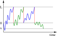
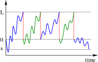
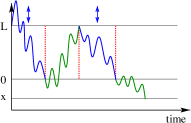
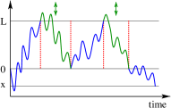
Figure 2: Schematic of diffusion with first-passage resetting. Shown are paths from $(0,0)$ to $(x,t)$ with: (a) an odd number or (b) an even number of reset events. We transform either the odd-numbered or the even-numbered pieces of the original path through the reflection $x(t)\rightarrow L-x(t)$ to yield free diffusion from either: (c) $(L,0)$ to $(x,t)$, or (d) $(0,0)$ to $(x,t)$. Summing over all numbers of reset events gives Eq. (5b).

For $y<0$, $\widetilde{P}(y,s)$ in Eq. (3) is factorizable:

$$\widetilde{P}(y,s) =\frac{1}{\sqrt{4Ds}}\!\left[\frac{e^{y}\!-\!e^{y-2y_{\scriptscriptstyle L}}}{1-e^{-y_{\scriptscriptstyle L}}}\right]=\frac{1}{\sqrt{4Ds}}\!\left[e^{y}\!+\!e^{(y-y_{\scriptscriptstyle L})}\right],$$ (5a)

and this latter form can be readily inverted to give

$$P(x,t)=\frac{1}{\sqrt{4\pi Dt}}\,\left[e^{-x^{2}/4Dt}+e^{-(x-L)^{2}/4Dt}\right]\quad x<0\,.$$ (5b)

Strikingly, this closed form represents the superposition of free diffusion paths to $(x,t)$ starting from $(0,0)$ and from $(L,0)$. This property may be derived by decomposing trajectories with resetting into a series of first-passage segments between each reset and then reflecting and translating them to obtain either a free diffusion path that starts at $(L,0)$ or at $(0,0)$ and propagates to $(x,t)$ as indicated in Fig. 2. We emphasize that this decomposition applies for any symmetric stochastic process.

A basic characteristic of regenerative processes is the number of reset events up to time $t$. The probability $Q_{n}$ for $n$ reset events is given by

$$Q_{n} =\text{Prob}(\geq n\ \text{resets})-\text{Prob}(\geq n\!+\!1\ \text{resets})$$

$$=\int_{0}^{t}\!dt^{\prime}\,\big{[}F_{n}(L,t^{\prime})-F_{n+1}(L,t^{\prime})\big{]}\,.$$

From our previous result that $F_{n}(L,t)=F_{1}(nL,t)$, we immediately have

$$Q_{n}=\mathrm{erf}\left(\frac{(n+1)L}{\sqrt{4Dt}}\right)-\mathrm{erf}\left(\frac{nL}{\sqrt{4Dt}}\right),$$ (6)

where $\mathrm{erf}$ is the Gauss error function.

We can compute $\mathcal{N}(t)\equiv\langle n\rangle$, the average number of reset events from (6), but it is quicker to express $\mathcal{N}(t)$ in terms of a backward renewal equation:

$$\mathcal{N}(t)=\int_{0}^{t}dt^{\prime}\,F_{1}(L,t^{\prime})\big{(}1+\mathcal{N}(t-t^{\prime})\big{)}\,.$$ (7)

Equation (7) accounts for the particle first hitting $L$ at any time $t^{\prime}<t$, then the process is renewed over the time range $t-t^{\prime}$, so there will be on average $1+\mathcal{N}(t-t^{\prime})$ resets. Taking the Laplace transform of (7) then leads to

$$\widetilde{\mathcal{N}}(s) =\frac{\widetilde{F}_{1}(L,s)}{s\,\big{[}1-\widetilde{F}_{1}(L,s)\big{]}}=\frac{e^{-y_{\scriptscriptstyle L}}}{s(1-e^{-y_{\scriptscriptstyle L}})},$$ (8)

from which we extract the long-time behavior of the average number of reset events by taking the $s\rightarrow 0$ limit. We thus find $\mathcal{N}(t)\simeq\sqrt{4Dt/\pi L^{2}}$.

Optimization in the Finite Interval: Let us now view the coordinate $x$ as the operating point of a mechanical system or a power grid with $x\in[0,L]$, and a control mechanism that acts upon $x$ in the form of a drift. It is desirable that the system operates close to the maximum operating point; that is, $x(t)$ near $L$. We therefore assign a reward that is proportional to $x(t)/L$. On the other hand, when $x$ reaches $L$ the system breaks down. Each breakdown incurs a cost $C$, after which the system is reset to the origin. The goal is to determine the optimal operation of this system, for which the objective function

$$\mathcal{F}=\,\lim_{T\rightarrow\infty}\,\frac{1}{T}\left[\frac{1}{L}\int_{0}^{T}x(t)\,dt-C\mathcal{N}(T)\right]$$ (9)

is maximized, with $\mathcal{N}(T)$ the number of breakdowns within a time $T$.

As a simple model, we posit that the coordinate $x$ changes in time according to diffusion, due to demand fluctuations, with superimposed drift. From a practical viewpoint, the drift should drive the system away from the breakdown point; that is, the control mechanism forestalls breakdowns. However, optimization arises for either sense of the drift. Mathematically, we need to solve the probability distribution of the particle which obeys the convection diffusion equation

$$\partial_{t}c+v\partial_{x}c=D\partial_{xx}c+\delta(x)(-D\partial_{x}c+vc)\rvert_{x=L}\,,$$ (10)

subject to the initial and boundary conditions

$$\begin{cases}{}\left(D\partial_{x}c-vc\right)\rvert_{x=0}=\delta(t)\,,\\ c(L,t)\,=\,c(x,0)=0\,.\end{cases}$$

Here, $c\equiv c(x,t)$ is the probability density, the subscripts denote partial differentiation, $D$ is the diffusion coefficient, and $v$ is the drift velocity. The delta-function term in (10) corresponds to the reinjection of the outgoing flux at $x=L$ to $x=0$, and the initial condition corresponds to starting the system at $(x,t)=(0,0)$.

This problem can be readily solved in the Laplace domain. As a preliminary, we first need to solve the simpler subproblem with no flux reinjection so that the delta-function term in (10) is absent. In this case, the concentration is De Bruyne et al. (2021)

$$\widetilde{c}_{0}(x,s) =\frac{2\,e^{vx/2D}\sinh\left[w(L-x)\right]}{\mathcal{M}}\,,$$ (11a)

where the subscript 0 denotes the concentration without flux reinjection, $${\text{Pe}}\equiv vL/2D w=\sqrt{v^{2}+4Ds}/2D \mathcal{M}=2Dw\cosh(Lw)+v\sinh(Lw) \widetilde{c}_{0} x=L$$ is the Péclet number, , and . From , the Laplace transform of the first-passage probability to is

$$\widetilde{F}_{1}(L,s) =\left(-D\partial_{x}\widetilde{c}_{0}+v\widetilde{c}_{0}\right)\rvert_{x=L}=\frac{2\,D\,w\,e^{{\text{Pe}}}}{\mathcal{M}}\,.$$ (11b)

With reinjection of the outgoing flux, the concentration obeys the renewal equations (2). In the Laplace domain and using $\widetilde{c}_{0}$ above, we find

$$\widetilde{c}(x,s)=\frac{\widetilde{c}_{0}(x,s)}{1-\widetilde{F}_{1}(L,s)}=\frac{2\,e^{vx/2D}\sinh[w(L-x)]}{\mathcal{M}-2D\,w\,e^{{\text{Pe}}}}\,.$$ (12)

where we substitute in Eqs. (11) to obtain the final result.

On a finite interval, diffusion with first-passage resetting is ergodic and admits a steady state Grigorescu and Kang (2002); Leung and Li (2008); Ben-Ari and Pinsky (2009). In the $s\to 0$ limit, the coefficient of the term proportional to $\frac{1}{s}$ in $\widetilde{c}(x,s)$ gives the steady-state concentration in the time domain, which is

$$c(x) \simeq\frac{1}{L}\times\frac{1\,-\,e^{-2{\text{Pe}}(L-x)/L}}{1\,-\,{\text{Pe}}^{-1}\,e^{-{\text{Pe}}}\,\sinh\left({\text{Pe}}\right)}\,,$$ (13)

from which the normalized first moment is

$$\frac{\langle x\rangle}{L}=\frac{1}{L}\int_{0}^{L}\!\!x\,c(x)\,dx=\frac{\left(2{\text{Pe}}^{2}-2{\text{Pe}}+1\right)\,e^{2{\text{Pe}}}-1}{2{\text{Pe}}\left[(2{\text{Pe}}-1)\,e^{2{\text{Pe}}}+1\right]}\,.$$ (14)

The average number of reset events $\mathcal{N}$ satisfies the backward renewal equation (7) and using $\widetilde{F}_{1}$ from (11b) we find

$$\widetilde{\mathcal{N}}(s) =\frac{2D\,w\,e^{{\text{Pe}}}}{s\,\left[\mathcal{M}-2Dw\,e^{{\text{Pe}}}\right]}\,.$$ (15a)

We now extract the long-time behavior for the average number of times that $$x=L s\rightarrow 0 \widetilde{\mathcal{N}}(s)$$ is reached by taking the limit of to give

$$\mathcal{N}(T) \simeq\frac{4{\text{Pe}}^{2}}{2{\text{Pe}}-1+e^{-2{\text{Pe}}}}\,\,\frac{T}{L^{2}/D}\,.$$ (15b)

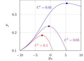
Figure 3: The objective function of Eq. (9) versus Péclet number Pe for different normalized cost values $C^{\prime}\equiv C/(L^{2}/D)$. Indicated on each curve is the optimal operating point.

Substituting these expressions for $\langle x\rangle/L$ and $\mathcal{N}$ into (9) immediately gives the objective function; representative plots are shown in Fig. 3. The salient feature is that there is an optimal operating Péclet number for each cost value. When the cost per breakdown is small, it is advantageous to run the system at positive Péclet number. Although there are many breakdowns, they are cheap, and there is a greater reward in pushing the system to the limit. Conversely, when the breakdown cost is high, the optimal operating point is at a negative Péclet number. Although there is little gain in operating the system at such a low level, the breakdown cost is so high that low-level operation is optimal.

When a mechanical system breaks down, there is downtime when repairs are effected before the system can be restarted. Such a delay, akin to the refractory period considered in Rotbart et al. (2015); Reuveni et al. (2014); Reuveni (2016); Evans and Majumdar (2011a), can be incorporated into our modeling by including a random delay after each resetting event. Thus when the particle reaches $x=L$ and is returned to $x=0$, it waits there a random time $\tau$ that is drawn from the exponential distribution $\sigma^{-1}e^{-\tau/\sigma}$ before moving again. Our formalism developed for instantaneous resetting can be naturally extended to resetting with delay—which might also be viewed as a so-called “sticky” Brownian motion Gallavotti and McKean (1972); Harrison and Lemoine (1981); Bou-Rabee and Holmes-Cerfon (2020) combined with resetting. The details are cumbersome, however, and we merely quote the main results. Upon including delay, the calculational steps that led to (14) now give De Bruyne et al. (2021)

$$\frac{\langle x\rangle}{L}=\frac{\left[(2{\text{Pe}}-2){\text{Pe}}+1\right]e^{2{\text{Pe}}}-1}{2\left[{\text{Pe}}(4\overline{\tau}\,{\text{Pe}}^{2}+2{\text{Pe}}-1)e^{2{\text{Pe}}}+{\text{Pe}}\right]}\,,$$ (16)

where $\overline{\tau}=D\sigma/L^{2}$ is a dimensionless measure of the delay time. Similarly, following the calculation that led to (15b), the average number of breakdowns is

$$\mathcal{N}=\frac{4{\text{Pe}}^{2}}{2{\text{Pe}}-1+4\overline{\tau}\,{\text{Pe}}^{2}+e^{-2{\text{Pe}}}}\,\frac{T}{L^{2}/D}\,.$$ (17)

This leads to an objective function whose qualitative features are similar to the no-delay case. The primary difference is that the optimal Péclet number and the corresponding optimal objective function $\mathcal{F}$ both decrease as the delay time is increased. Indeed, delay reduces the number of breakdowns but also induces the coordinate to remain closer to the origin. In the limit where the delay is extremely long, the optimal Péclet number will be small and will almost not depend on the cost per breakdown, as the particle almost never hits the resetting boundary.

In summary, triggering the reset of a diffusing particle by a first-passage event leads to rich features. On the infinite line, the probability distribution is exactly calculable and can be understood in terms of a subtle path decomposition. In a finite domain $[0,L]$, there exists an optimal bias velocity that maintains the system at maximum performance—close to the peak operating point of $x=L$ while minimizing the number of breakdowns.

The formalism developed here can be extended to systems with multiple degrees of freedom, such as a power grid, where the breakdown in one coordinate induces a breakdown in another coordinate. Another promising direction is to incorporate the possibility of partial versus complete repair Rausand and Høyland (2003). After partial repair, the operating range of the system is reduced, so that the next breakdown is more likely to occur sooner. On the other hand, there will be a smaller penalty associated with partial repair. This perspective may allow one to optimize both the frequency and magnitude of repair costs.

More generally, first-passage resetting may lead to intriguing statistical features in problems in control theory and management science (where fluctuations of inventory or cash fund levels are typically modeled by random walks or Brownian motion, and there generally exists a maximal capacity that one seeks to use optimally Harrison et al. (1983); Buckholtz et al. (1983)) or in biology (where allele frequencies in population genetics models evolve according to diffusion, with “killing” when a frequency reaches a limit level Tavaré (1979); Goel and Richter-Dyn (2016)).