Langevin Simulations of the Half-Filled Cubic Holstein Model

Abstract

Over the past several years, reliable Quantum Monte Carlo results for the charge density wave transition temperature $T_{\rm cdw}$ of the half-filled two dimensional Holstein model in square and honeycomb lattices have become available for the first time. Exploiting the further development of numerical methodology, here we present results in three dimensions, which are made possible through the use of Langevin evolution of the quantum phonon degrees of freedom. In addition to determining $T_{\rm cdw}$ from the scaling of the charge correlations, we also examine the nature of charge order at general wave vectors for different temperatures, couplings, and phonon frequencies, and the behavior of the spectral function and specific heat.

Introduction. Substantial effort has been devoted to developing and using Quantum Monte Carlo (QMC) techniques to study the physics of interacting electrons. Auxiliary field methods formulated in real space, like Determinant Quantum Monte Carlo (DQMC) Blankenbecler et al. (1981); White et al. (1989); Sorella et al. (1989), can determine correlations on clusters of several hundreds of sites. However, unbiased approaches to studying electron correlations, such as DQMC, can be severely limited by the sign problem Loh et al. (1990); Iglovikov et al. (2015), unless additional constraints are imposed Zhang et al. (1997). The Dynamic Cluster Approximation Maier et al. (2005) and Cluster Dynamical Mean Field Theory Capone and Kotliar (2007); Gull et al. (2007) generalize single site Dynamical Mean Field theory Metzner and Vollhardt (1989); Jarrell (1992); Georges and Kotliar (1992); Georges et al. (1996); Jarrell et al. (2001); Kyung et al. (2006) to finer momentum grids and generally have a more benign sign problem than DQMC, allowing them to access lower temperatures and/or more complex (e.g. multi-band) models. Diagrammatic QMC is another relatively new technology which is currently being developed Kozik et al. (2010, 2013). Despite the numerical challenges, QMC applied to models with electron-electron interactions, like the Hubbard model, has resulted in considerable qualitative insight into phenomena such as the Mott transition, magnetic order, and, to a somewhat lesser extent, exotic superconductivity (SC) Scalapino (1994) which arise from electron-electron interactions in real materials Dagotto (2005).

Analogous strong correlation effects can arise in solids due to electron-phonon coupling, including SC and charge density wave (CDW) formation; this is the type of interaction we examine in this paper. A simple model where such effects can be studied is the Holstein Hamiltonian Holstein (1959). Early QMC work in two dimensions near half-filling  Scalettar et al. (1989a); Noack et al. (1991); Vekić et al. (1992); Niyaz et al. (1993); Marsiglio (1990); Hohenadler et al. (2004) examined CDW formation and its competition with SC. A second generation of simulations has considerably improved the quantitative accuracy of results looking at both finite temperature Weber and Hohenadler (2018); Chen et al. (2018); Cohen-Stead et al. (2019) and quantum critical point Chen et al. (2019); Zhang et al. (2019) physics in two spatial dimensions on square and honeycomb lattices. Much of this progress has been possible thanks to newer QMC methods such as continuous time Weber and Hohenadler (2018) and self-learning Monte Carlo Xu et al. (2017); Chen et al. (2018). However, despite these improvements in effective update schemes, the cubic scaling with lattice size $N$ of real space QMC methods employed in existing work has precluded similar studies in three dimensions.

We report here QMC simulations of the half-filled Holstein model on cubic lattices as large as $N=14^{3}$ sites. These studies are made possible by employing a linear-scaling QMC method based on a Langevin evolution of the phonon degrees of freedom Batrouni and Scalettar (2019a, b); Karakuzu et al. (2018); Beyl et al. (2018). The large linear sizes that are accessible allow us to perform the finite size scaling needed to extract the CDW transition temperature $T_{\rm cdw}$ and also obtain the momentum dependence of the charge structure factor $S({\bf k})$ to reasonable resolution. We supplement the extraction of $T_{\rm cdw}$ from $S_{\rm cdw}\equiv S(\pi,\pi,\pi)$ with calculation of the specific heat and spectral function, and show that, while they provide a less precise determination of $T_{\rm cdw}$, their features are consistent with those obtained from $S_{\rm cdw}$.

Model and Methods. The Holstein Hamiltonian,

$$\mathcal{\hat{H}}= -t\sum_{\langle\mathbf{i},\mathbf{j}\rangle,\sigma}\big{(}\hat{c}^{\dagger}_{\mathbf{i}\sigma}\hat{c}^{\phantom{\dagger}}_{\mathbf{j}\sigma}+{\rm h.c.}\big{)}-\mu\sum_{\mathbf{i},\sigma}\hat{n}_{\mathbf{i},\sigma}$$

$$+\frac{1}{2}\sum_{\mathbf{i}}\hat{P}^{2}_{\mathbf{i}}+\frac{\omega_{\,0}^{2}}{2}\sum_{\mathbf{i}}\hat{X}^{2}_{\mathbf{i}}+\lambda\sum_{\mathbf{i},\sigma}\hat{n}_{\mathbf{i},\sigma}\hat{X}_{\mathbf{i}}\,\,,$$ (1)

describes the coupling of electrons, with creation and destruction operators $\hat{c}^{\dagger}_{\mathbf{i}\sigma},\hat{c}^{\phantom{\dagger}}_{\mathbf{i}\sigma}$, to dispersionless phonon degrees of freedom $\hat{P}_{\mathbf{i}},\hat{X}_{\mathbf{i}}$, with the phonon mass normalized to $M=1$. The parameter $t$ multiplies a near-neighbor hopping (kinetic energy) term. We set $t=1$ as our unit of energy, resulting in an electronic bandwidth for the cubic lattice equal to $W=12$. The coupling between the phonon displacement and electron density on site $\mathbf{i}$ is controlled by $\lambda$ while the chemical potential, $\mu$, tunes the filling. In this study we focus on half-filling, obtained by setting $\mu=-\lambda^{2}/\omega_{0}^{2}$, and report results in terms of a dimensionless electron-phonon coupling constant $\lambda_{D}=\lambda^{2}/(\omega_{0}^{2}W)$. Despite its simplifications, the Holstein model captures many qualitative features of electron-phonon physics, including polaronic effects in the dilute limit Romero et al. (1999); Ku et al. (2002); Marchand and Berciu (2013), SC and CDW formation, and their competition Scalettar et al. (1989b); Aubry et al. (1989); Zheng and Zhu (1997); Grzybowski and Micnas (2007); Esterlis et al. (2018); Weber and Hohenadler (2018); Chen et al. (2019); Zhang et al. (2019).

The fermionic degrees of freedom appear only quadratically in the Holstein model, Eq. (Langevin Simulations of the Half-Filled Cubic Holstein Model). Consequently, the fermions can be “integrated out” resulting in the product of two identical matrix determinants which are nontrivial functions of the space and imaginary time dependent phonon field. The product of the two identical determinants is positive; thus there is no sign problem. Most prior numerical studies of the Holstein model employed DQMC, which explicitly calculates changes in the determinant as the phonon field is updated. At fixed temperature, DQMC scales cubically in the number of sites $N$, and hence as $L^{9}$, where $L$ is the linear system size in 3D. This limits DQMC simulations in three dimensions to relatively small $L$.

Instead, we use a method based on Langevin updates which exhibits linear near scaling in $N$. Such methods were first formulated for lattice gauge theories Batrouni et al. (1985); Davies et al. (1986); Batrouni (1987). Attempts to simulate the Hubbard Hamiltonian with Langevin updates were limited to relatively weak coupling and high temperature by the ill-conditioned nature of the matrices, due to rapid fluctuations of the sampled Hubbard-Stratonvich fields in the imaginary time direction Scalettar et al. (1986). However, in the Holstein model the sampled phonon fields have an associated kinetic energy cost that moderates these fluctuations, giving rise to better conditioned matrices.

Here we briefly discuss the key steps in the algorithm and leave the details to Refs. Batrouni and Scalettar (2019a, b). The partition function for the Holstein model is first expressed as a path integral in the phonon coordinates, $x({\bf i},\tau)$, by discretizing the inverse temperature $\beta=L_{\tau}\Delta\tau$. After performing the trace over the fermion coordinates, the phonon action ${\cal S}$ includes a term ${\rm ln}\,({\rm det}{\cal M})$ where ${\cal M}$ is a matrix of dimension $NL_{\tau}$. The phonon field is then evolved in a fictitious Langevin time $t$ with $x({\bf i},\tau,t)$ moving under a force $\partial{\cal S}/\partial{x({\bf i},\tau,t)}$ and a stochastic noise term. The part of the derivative of ${\cal S}$ which involves ${\rm ln}\,({\rm det}{\cal M})$ is evaluated with a stochastic estimator. It is necessary to compute ${\cal M}^{-1}$ acting on vectors of length $NL_{\tau}$, which is done using the conjugate gradient (CG) method. An essential refinement of the algorithm is the application of Fourier Acceleration Batrouni et al. (1985); Davies et al. (1986); Batrouni (1987) to reduce critical slowing down resulting from the slow phonon dynamics in imaginary time.

Elements of the fermionic Green function are also obtained with a stochastic estimator. Once evaluated, one can measure all physical observables. We focus here on the charge structure factor,

$$S({\bf k}) \equiv\sum_{\bf r}c({\bf r})\,e^{i{\bf k}\cdot{\bf r}},$$

$$c({\bf r}) =\langle\,n_{\bf j+r}n_{\bf j}\,\rangle,$$ (2)

($n_{\bf j}=n_{{\bf j}\uparrow}+n_{{\bf j}\downarrow}$), and the specific heat $C=d\langle E\rangle/dT$. We also obtain the momentum integrated spectral function $A(\omega)$, the analog of the density of states in the presence of interactions, by analytic continuation of the Green function via the maximum entropy method Gubernatis et al. (1991); Jarrell and Gubernatis (1996).

Correlation Length and Charge Structure Factor. At half-filling on a bipartite lattice the formation of a CDW phase is the fundamental ordering tendency of the Holstein model. At intermediate temperatures we observe the formation of local pairs due to the effective on-site attraction $U_{\rm eff}=-\lambda^{2}/\omega_{0}^{2}$, between up and down electrons. At lower $T$, the positions of the pairs become correlated, since the lowering of energy by virtual hopping is maximized by $-4t^{2}/U_{\rm eff}$ if each pair is surrounded by empty sites. A clear signature of this low temperature physics is seen in the heat capacity $C(T)$ as the temperature is lowered, which has a sharp peak at $T\sim 0.28$ corresponding to the CDW phase transition, as shown in Fig. 1.

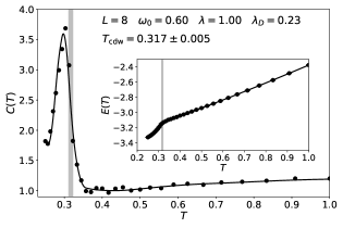
Figure 1: Specific heat $C(T)$ as a function of temperature $T$. The low temperature peak corresponds to the onset of charge ordering. Here $\lambda_{D}=0.23,\omega_{0}=0.60$ and the lattice size is $N=8^{3}$.

It is also possible to detect the formation of this low temperature CDW phase by studying the density-density correlation function, and its Fourier transform, the charge structure factor, $S({\bf k})$. In Fig. 2 we show $S({\bf k})$, Eq. (2), versus ${\bf k}$ for different $T=\beta^{-1}$ and $\lambda_{D}=0.33\ (\omega_{0}=0.5,\ \lambda=1.0)$. We see that, as $T$ is lowered, the peak height at ${\bf k}=(\pi,\pi,\pi)$ increases by two orders of magnitude. The value of $\beta$ for which the height increases most rapidly provides a rough value for the transition temperature, which can be more precisely determined via finite size scaling (Fig. 4).

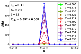
Figure 2: Charge structure factor as a function of momentum for different inverse temperature $\beta$ at fixed $\lambda_{D}=0.33$ and $\omega_{0}=0.5$. As $T$ decreases, a peak develops at ${\bf k}=(\pi,\pi,\pi)$. The most rapid growth is for $T\sim 0.37$-$0.40$. Finite size scaling analysis of the crossings of $S_{\rm cdw}$ in Fig. 4, precisely identifies $T_{c}\sim 0.392\pm 0.008$.

In real space, the density-density correlation function exhibits a pattern which oscillates in sign on the two sublattices, consistent with dominant ordering at ${\bf k}=(\pi,\pi,\pi)$ seen in Fig. 2. Above $T_{c}$, the correlations die off exponentially, with a correlation length $\xi$ which grows as $T\rightarrow T_{c}$. (See Supplemental Materials.) In finite size simulations, $\xi$ will be bounded by the system size $L$, but one can nevertheless estimate it via Sandvik (2010),

$$\xi=\frac{L}{2\pi}\sqrt{\frac{S(q_{1})/S(q_{2})-1}{4-S(q_{1})/S(q_{2})}}\,\,,$$ (3)

where $q_{1}=(\pi,\pi,\pi-\frac{2\pi}{L})$ and $q_{2}=(\pi,\pi,\pi-\frac{4\pi}{L})$ are the two closest wave vectors to the ordering vector ${\bf k}=(\pi,\pi,\pi)$.

Figure 3 shows the ratio $\xi/L$ as a function of temperature for three lattice sizes $L=8,10,12$. $\xi/L$ exhibits a characteristic peak, which sharpens with increasing lattice size. In the following section, we will present data indicating $T_{\rm cdw}=0.31$ which is consistent with the peak in finite lattice sizes approaching $T_{c}$ from above in our data as well.

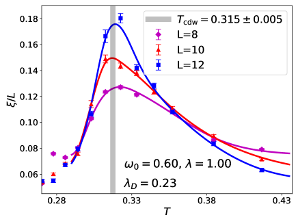
Figure 3: Correlation length obtained from Eq. (3) with $\omega_{0}=0.6,\lambda=1.0\,\,(\lambda_{D}=0.23)$. Shaded gray bar shows the value of $T_{c}$ obtained from a finite-size scaling analysis of the CDW structure factor (Fig. 4).

CDW Transition. Having seen the essential qualitative effects of the electron-phonon coupling, we now perform finite size scaling to locate the transition precisely. The three panels of Fig. 4 exhibit the steps in this process. The upper left panel (a) exhibits raw data for $S_{\rm cdw}$ versus inverse temperature $\beta$. At high $T$ (small $\beta$) the values of $S_{\rm cdw}$ for different system sizes coincide with each other, because the charge correlations are short ranged and the additional large distance values in the sum over ${\bf r}$ in Eq. (2), present as $L$ increases, make no contribution. However, as $T$ decreases ($\beta$ increases) the correlation length reaches the lattice size, and values of $S_{\rm cdw}$ now become sensitive to the cut-off $L$. As a consequence, a crude estimate of $T_{\rm cdw}$ can already be made as the temperature at which the curves begin to separate, i.e. $T_{\rm cdw}\sim 0.31\;(\beta_{c}\sim 3.2)$.

A much more accurate determination of $T_{\rm cdw}$ is provided by making a crossing plot (Fig. 4c) of $S_{\rm cdw}L^{2\beta/\nu-D}$ versus $\beta$. Curves for different lattice sizes $L$ should cross at $\beta_{c}=1/T_{\rm cdw}$. In this analysis we make use of the expected universality class of the transition, the 3D Ising model, to provide values for the exponents $\beta=0.326$ and $\nu=0.63$. We conclude $T_{\rm cdw}=0.315\pm 0.005$. Finally, Fig. 4(c) gives the full scaling collapse, using $T_{\rm cdw}$ from panel (b) and again employing 3D Ising exponents.

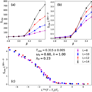
Figure 4: Finite size scaling analysis of the CDW structure factor. Panel (a) contains the raw (unscaled) data. $S_{\rm cdw}$ is independent of $L$ for small $\beta$ where the correlation length is short. At large $\beta$, $S_{\rm cdw}$ grows with $L$. Panel (b) scales $S_{\rm cdw}$ only. The result is a crossing plot which yields the critical inverse temperature $\beta_{c}\,t=3.15\pm 0.05$. The main panel (c) shows a full scaling plot where the data collapse in a range of inverse temperatures near the critical point. Holstein model parameters are $\omega_{0}=0.60,\lambda=1.0$ so that $\lambda_{D}=0.23$.

Combining plots like those of Fig. 4 for different values of $\lambda$ and $\omega_{0}$ allows us to obtain the finite temperature phase diagram of the 3D Holstein model, Fig. 5, which is the central result of this paper. We see that $T_{c}$ is increased by roughly a factor of two in going from various 2D geometries (square Weber and Hohenadler (2018), Lieb fen , and honeycomb Chen et al. (2019); Zhang et al. (2019)) to 3D. This increase is quite similar to that of going from 2D square ($T_{c}\sim 2.27$) to 3D cubic ($T_{c}\sim 4.51$) for the CDW transition of classical lattice gas (Ising) model.

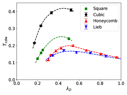
Figure 5: Phase diagram of the 3D Holstein model on a cubic lattice as a function of $\lambda_{D}$, with $\lambda=1$ held fixed. For comparison, critical temperatures on three 2D lattice geometries, square, honeycomb, and Lieb are also given.

Spectral Function. The preceding results are all obtained with imaginary time-independent Green functions. More generally, one can consider,

$$G({\bf k},\tau)\equiv\langle c({\bf k},\tau)c^{\dagger}({\bf k},0)\rangle=\int d\omega A({\bf k},\omega)\,\frac{e^{-\omega\tau}}{e^{\beta\omega}+1}$$ (4)

to determine the spectral function $A({\bf k},\omega)$. This involves inverting the integral relation in Eq. (4) using analytic continuation Gubernatis et al. (1991); Jarrell and Gubernatis (1996). This is the first use of our Langevin approach for dynamical behavior. Figure 6 shows $A(\omega)$ for several different temperatures at fixed $\omega_{0}=0.7,\lambda_{D}=0.17$. At high temperatures ($\beta=3$ and $4$) the main effect of the electron-phonon interaction is to increase the spectral function somewhat in the region close to the band edges $\omega=\pm 6t$. The renormalized bandwidth is remarkably unchanged from that of free electrons on a cubic lattice, $W=12t$. When $T$ reaches the CDW ordering temperature, $\beta\sim 5$ (see Fig. 5) $A(\omega=0)$ develops a pronounced dip. This suppression continues to increase until, at $\beta=8$, $A(\omega=0)$ vanishes. This sequence, in which a dip first signals entry into the CDW phase, is consistent with the trends reported in Cohen-Stead et al. (2019).

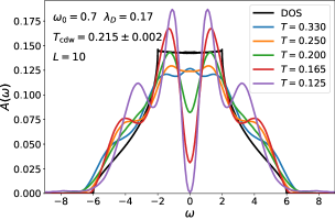
Figure 6: Momentum integrated spectral function $A(\omega)$. Here $\omega_{0}=0.7,\lambda_{D}=0.17$, and the lattice size $N=10^{3}$. A suppression of $A(\omega=0)$ coincides with reaching $\beta_{c}\sim 5$. (See Fig. 5.) A full gap develops at a somewhat lower temperature. Also shown, for comparison, is the density of states of non-interacting electrons ($\lambda_{D}=0$) hopping on a cubic lattice.

Conclusions. We have used a new Langevin QMC method to study the Holstein Hamiltonian on a three-dimensional cubic lattice. This new approach allows us to access much larger lattice sizes, enabling us to perform a reliable finite size scaling analysis to determine the CDW transition temperature. Using this method, we obtained results that, in momentum space, were sufficient to resolve the width of the charge structure factor peak and the smearing of the Fermi surface by electron-phonon interactions. The specific heat and spectral function provide useful alternate means to examine the low temperature properties. Their behavior is consistent with that seen by direct observation of charge correlations.

While a single band model of interacting electrons does seem to provide a reasonably accurate representation of cuprate physics Scalapino (1994) (although not that of the iron-pnictides), realistic CDW materials generally have much richer band structures. Since, at a formal level, additional sites and additional orbitals are equivalent in real-space QMC simulations, an ability to simulate larger spatial lattices also opens the door to the study of more complex CDW systems. Of course, the accurate description of these materials requires not only several electronic bands, but also a refinement of the description of the phonons and electron-phonon coupling, which are also treated at a very simple level in the Holstein Hamiltonian. Initial steps to include phonon dispersion have recently been made Costa et al. (2018). However, refinements to the electron-phonon coupling such as a momentum dependent $\lambda({\bf q})$ remain a challenge to simulations because of the phase separation that results in the absence of electron-electron repulsion Xiao et al. (2019).

Acknowledgements: The work of B.C-S. and R.T.S was supported by the grant DE‐SC0014671 funded by the U.S. Department of Energy, Office of Science. K.B. acknowledges support from the center of Materials Theory as a part of the Computational Materials Science (CMS) program, funded by the U.S. Department of Energy, Office of Science. G.G.B. is partially supported by the French government, through the UCAJEDI Investments in the Future project managed by the National Research Agency (ANR) with the reference number ANR-15-IDEX-01. C.C. and Z.Y.M. acknowledge the supports from MOST China through the National Key Research and Development Program (Grant No. 2016YFA0300502) and Research Grants Council of Hong Kong SAR China through 17303019 and thank the Center for Quantum Simulation Sciences in the Institute of Physics, Chinese Academy of Sciences, the Computational Initiative at the Faculty of Science at the University of Hong Kong, the Platform for Data-Driven Computational Materials Discovery at the Songshan Lake Materials Laboratory, Guangdong, China and the National Supercomputer Centers in Tianjin and Guangzhou for their technical support and generous allocation of CPU time.

References

- Blankenbecler et al. (1981) R. Blankenbecler, D. J. Scalapino, and R. L. Sugar, Phys. Rev. D 24, 2278 (1981).
- White et al. (1989) S. R. White, D. J. Scalapino, R. L. Sugar, E. Y. Loh, J. E. Gubernatis, and R. T. Scalettar, Phys. Rev. B 40, 506 (1989).
- Sorella et al. (1989) S. Sorella, S. Baroni, R. Car, and M. Parinello, Europhys. Lett. 8, 663 (1989).
- Loh et al. (1990) E. Y. Loh, J. E. Gubernatis, R. T. Scalettar, S. R. White, D. J. Scalapino, and R. L. Sugar, Phys. Rev. B 41, 9301 (1990).
- Iglovikov et al. (2015) V. I. Iglovikov, E. Khatami, and R. T. Scalettar, Phys. Rev. B 92, 045110 (2015).
- Zhang et al. (1997) S. Zhang, J. Carlson, and J. Gubernatis, Phys. Rev. B 55, 7464 (1997).
- Maier et al. (2005) T. Maier, M. Jarrell, T. Pruschke, and M. Hettler, Rev. Mod. Phys. 77, 1027 (2005).
- Capone and Kotliar (2007) M. Capone and G. Kotliar, J. Mag. and Mag. Mat. 310, 529 (2007).
- Gull et al. (2007) E. Gull, M. Ferrero, O. Parcollet, A. Georges, and A. Millis, Phys. Rev. B 82, 155101 (2007).
- Metzner and Vollhardt (1989) M. Metzner and D. Vollhardt, Phys. Rev. Lett. 62, 324 (1989).
- Jarrell (1992) M. Jarrell, Phys. Rev. Lett. 69, 168 (1992).
- Georges and Kotliar (1992) A. Georges and G. Kotliar, Phys. Rev. B 45, 6479 (1992).
- Georges et al. (1996) A. Georges, G. Kotliar, W. Krauth, and M. Rozenberg, Rev. Mod. Phys. 68, 13 (1996).
- Jarrell et al. (2001) M. Jarrell, T. Maier, C. Huscroft, and S. Moukouri, Phys. Rev. B 64, 195130 (2001).
- Kyung et al. (2006) B. Kyung, G. Kotliar, and A.-M. Tremblay, Phys. Rev. B 73, 205106 (2006).
- Kozik et al. (2010) E. Kozik, K. V. Houcke, E. Gull, L. Pollet, N. Prokofév, B. Svistunov, and M. Troyer, Europhys. Lett. 90, 10004 (2010).
- Kozik et al. (2013) E. Kozik, E. Burovski, V. Scarola, and M. Troyer, Phys. Rev. B 87, 205102 (2013).
- Scalapino (1994) D. Scalapino, Proceedings of the International School of Physics, edited by R. A. Broglia and J. R. Schrieffer, North-Holland, New York; and references cited therein (1994).
- Dagotto (2005) E. Dagotto, Science 309, 257 (2005).
- Holstein (1959) T. Holstein, Annals of Physics 8, 325 (1959).
- Scalettar et al. (1989a) R. T. Scalettar, N. E. Bickers, and D. J. Scalapino, Phys. Rev. B 40, 197 (1989a).
- Noack et al. (1991) R. Noack, D. Scalapino, and R. Scalettar, Phys. Rev. Lett. 66, 778 (1991).
- Vekić et al. (1992) M. Vekić, R. Noack, and S. White, Phys. Rev. B 46, 271 (1992).
- Niyaz et al. (1993) P. Niyaz, J. Gubernatis, R. Scalettar, and C. Fong, Phys. Rev. B 48, 16011 (1993).
- Marsiglio (1990) F. Marsiglio, Phys. Rev. B 42, 2416 (1990).
- Hohenadler et al. (2004) M. Hohenadler, H. G. Evertz, and W. von der Linden, Phys. Rev. B 69, 024301 (2004).
- Weber and Hohenadler (2018) M. Weber and M. Hohenadler, Phys. Rev. B 98, 085405 (2018).
- Chen et al. (2018) C. Chen, X. Y. Xu, J. Liu, G. Batrouni, R. Scalettar, and Z. Y. Meng, Phys. Rev. B 98, 041102 (2018).
- Cohen-Stead et al. (2019) B. Cohen-Stead, N. Costa, E. Khatami, and R. Scalettar, Phys. Rev. B 100, 045125 (2019).
- Chen et al. (2019) C. Chen, X. Xu, Z. Meng, and M. Hohenadler, Phys. Rev. Lett. 122, 077601 (2019).
- Zhang et al. (2019) Y. Zhang, W. Chiu, N. Costa, G. Batrouni, and R. Scalettar, Phys. Rev. Lett. 122, 077602 (2019).
- Xu et al. (2017) X. Y. Xu, Y. Qi, J. Liu, L. Fu, and Z. Y. Meng, Phys. Rev. B 96, 041119 (2017).
- Batrouni and Scalettar (2019a) G. G. Batrouni and R. T. Scalettar, Phys. Rev. B 99, 035114 (2019a).
- Batrouni and Scalettar (2019b) G. G. Batrouni and R. T. Scalettar, Comm. Comp. Phys. 1290, 012004 (2019b).
- Karakuzu et al. (2018) S. Karakuzu, K. Seki, and S. Sorella, Phys. Rev. B 98, 201108 (2018).
- Beyl et al. (2018) S. Beyl, F. Goth, and F. F. Assaad, Phys. Rev. B 97, 085144 (2018).
- Romero et al. (1999) A. Romero, D. Brown, and K. Lindenberg, Phys. Rev. B 60, 14080 (1999).
- Ku et al. (2002) L. Ku, S. Trugman, and J. Bonca, Phys. Rev. B 65, 174306 (2002).
- Marchand and Berciu (2013) D. J. J. Marchand and M. Berciu, Phys. Rev. B 88, 060301 (2013).
- Scalettar et al. (1989b) R. Scalettar, D. Scalapino, and N. Bickers, Phys. Rev. B 40, 197 (1989b).
- Aubry et al. (1989) S. Aubry, P. Quemerais, and J. Raimbault, Charge density wave and superconductivity in the Holstein model, Tech. Rep. (Laboratoire Leon Brillouin (LLB)-Centre d’Etudes Nucleaires de Saclay, 1989).
- Zheng and Zhu (1997) H. Zheng and S. Y. Zhu, Phys. Rev. B 55, 3803 (1997).
- Grzybowski and Micnas (2007) P. Grzybowski and R. Micnas, Acta Physica Polonica A 111, 455 (2007).
- Esterlis et al. (2018) I. Esterlis, B. Nosarzewski, E. W. Huang, B. Moritz, T. P. Devereaux, D. J. Scalapino, and S. A. Kivelson, Phys. Rev. B 97, 140501 (2018).
- Batrouni et al. (1985) G. Batrouni, G. Katz, A. Kronfeld, G. Lepage, B. Svetitsky, and K. Wilson, Phys. Rev. D 32, 2736 (1985).
- Davies et al. (1986) C. Davies, G. Batrouni, A. K. G. Katz, P. Lepage, P. Rossi, B. Svetitsky, and K. Wilson, J. Stat. Phys. 43, 1073 (1986).
- Batrouni (1987) G. G. Batrouni, Nucl. Phys. A461, 351c (1987).
- Scalettar et al. (1986) R. Scalettar, D. Scalapino, and R. Sugar, Phys. Rev. B 34, 7911 (1986).
- Gubernatis et al. (1991) J. Gubernatis, M. Jarrell, R. Silver, and D. S. Sivia, Phys. Rev. B 44, 6011 (1991).
- Jarrell and Gubernatis (1996) M. Jarrell and J. Gubernatis, Phys. Rep. 269, 133 (1996).
- Sandvik (2010) A. Sandvik, AIP Conference Proceedings 1297, 135 (2010).
- (52) C. Feng, H.M. Guo, and R.T. Scalettar, work in progress.
- Costa et al. (2018) N. Costa, T. Blommel, W. Chiu, G. Batrouni, and R. Scalettar, Phys. Rev. Lett. 120, 187003 (2018).
- Xiao et al. (2019) B. Xiao, F. Hébert, G. Batrouni, and R. Scalettar, Phys. Rev. B 99, 205145 (2019).