Acousto-optic modulation in lithium niobate on sapphire

Abstract

We demonstrate acousto-optic phase modulators in X-cut lithium niobate films on sapphire, detailing the dependence of the piezoelectric and optomechanical coupling coefficients on the crystal orientation. This new platform supports highly confined, strongly piezoelectric mechanical waves without suspensions, making it a promising candidate for broadband and efficient integrated acousto-optic devices, circuits, and systems.

The demonstration of low-loss nanophotonic waveguides Wang et al. (2014) in high-quality, single-crystal films of lithium niobate (LN) Levy et al. (1998) has led to a surge in the development of electro-optic and nonlinear optical devices. Because of their small mode area, these waveguides exhibit large nonlinear interactions and require less energy to parametrically drive, underlying recent progress in LN frequency combs Yu et al. (2019), second-harmonic generation Rao et al. (2016a); Chang et al. (2016), and high-speed electro-optic modulators Rao et al. (2016b); Wang et al. (2018).

In addition to the large $\chi^{\left(2\right)}$ nonlinearity and electro-optic effect that make LN an attractive material for optics, LN is a low-loss mechanical material with strong piezoelectric coupling, properties that are necessary for making broadband and efficient acousto-optic modulators (AOMs). In parallel to the development of nanophotonics in thin film LN, strongly piezoelectric, low-loss resonators Olsson III et al. (2014); Pop et al. (2017) and delay-lines Manzaneque et al. (2019) have been demonstrated and wavelength-scale waveguides efficiently transduced Dahmani et al. (2019) in suspended films. Using these piezoelectric devices, suspended LN AOMs have realized low-power microwave-to-optical conversion in pursuit of quantum optical interconnects Shao et al. (2019); Jiang et al. (2020).

While suspended devices are at the forefront of low-power acousto-optics, suspensions add fabrication constraints that inhibit the development of complex photonic and phononic circuits and systems. Another approach to co-localize optical and mechanical waves is to employ the Rayleigh-like surface acoustic wave (SAW) which is confined to the surface in any material platform. These SAWs can modulate a variety of optical structures including resonators Tadesse and Li (2014); waveguides as recently used to demonstrate non-magnetic isolation Kittlaus et al. (2020); Mach-Zehnders for intensity modulators van der Poel et al. (2007); Van Der Slot, Porcel, and Boller (2019); Cai et al. (2019) and acousto-optic gryoscopes Mahmoud et al. (2018a, b); and arrayed waveguide gratings Crespo-Poveda et al. (2015, 2016) with Refs. Mahmoud et al. (2018a, b); Cai et al. (2019) using LN-on-insulator. But LN-on-insulator has a fundamental drawback. Analogous to the advantage of high confinement in electro-optics and nonlinear optics, high mechanical confinement is necessary for broadband electromechanical transduction as well as for efficient optomechanical modulation. In LN-on-insulator, however, as the mechanical wavelength approaches the thickness of the LN film, the mechanical wave leaks out of the LN and into the silica which supports slower mechanical waves. This can be addressed by replacing the insulator substrate with a material with higher sound velocities enabling high-confinement mechanical waves in the thin-film device layer.

Here we explore integrated acousto-optic modulation in X-cut, thin-film LN bonded to sapphire with a focus on verifying the piezoelectric and acousto-optic properties of our film. This new platform enables high-confinement optical waveguides from the near-infrared to the visible and, in addition to Rayleigh-like SAWs, supports guided horizontal shear (SH) waves that exhibit large electromechanical coupling coefficients $k_{\textrm{eff}}^{2}$ at GHz-frequencies. Compared to related efforts in other platforms making use of aluminum nitride, silicon, or gallium arsenide, this platform enables strong confinement of the mechanical waves without suspensions, setting the stage for complex phononic circuitry and systems. We demonstrate a surface wave acousto-optic phase modulator (discussed in Section I) utilizing the Rayleigh and SH modes near $700$ and $800\text{\,}\mathrm{MHz}$, respectively, and characterize them in the telecom C-band. By comparing simulations and measurements of the piezoelectric coupling coefficient $k_{\textrm{eff}}$ (Section II.1) and the optomechanical coupling coefficient $g$ (Section II.2), we show the degree to which these bonded films retain their piezoelectric and acousto-optic properties. The acousto-optic portion of the study is similar to recent work by Khan et al. which extracted the dominant elasto-optic coefficients for waveguides patterned in sputtered arsenic trisulfide films Khan et al. (2019). Furthermore, we show that at GHz frequencies as the wavelength approaches the LN film thickness, the piezoelectric coupling of the SH wave quickly increases with $k_{\textrm{eff}}^{2}$ exceeding $10\%$ just above $2\text{\,}\mathrm{GHz}$.

I Modeling SAW phase modulators

The surface wave phase modulator shown in Figure 1a is a simple acousto-optic device with two parts : a piezoelectric transducer to generate mechanical waves and an optical ridge waveguide modulated by these waves. Surface waves are generated by an interdigitated transducer (IDT) with phase fronts parallel to an optical ridge waveguide. These surface waves modulate the effective index of refraction $n_{\textrm{eff}}$ of the waveguide and therefore the phase of light transmitted through the device.

The piezoelectric transducer is characterized by two numbers, the effective piezoelectric coupling coefficient $k_{\textrm{eff}}$ and the transmission coefficient $t_{\textrm{b}\upmu}$ from microwaves incident on the IDT to phonons in a specific mechanical mode and direction Hashimoto and Hashimoto (2000); Hashimoto (2009); Dahmani et al. (2019). For our purposes, the most important characteristic of the ridge waveguide is the optomechanical coupling coefficient $g$ which has units of $\left(\textrm{W}\cdot\textrm{m}\right)^{-1/2}$ and is defined in Appendix A. Of these figures, $k_{\textrm{eff}}$ and $g$ are proportional to the piezoelectric and photoelastic tensors Andrushchak et al. (2009), respectively, and so can be used to characterize the quality of the bonded film and platform. For this reason, they are the focus of our study. But in order to extract $g$ from optical measurements of the modulation index $h_{\textrm{ao}}$, we also need to determine $t_{\textrm{b}\upmu}$.

First we consider numerical analyses of the transducer in Figure 1b, focusing on $k_{\textrm{eff}}$ before considering $t_{\textrm{b}\upmu}$. A large $k_{\textrm{eff}}$ is essential for making small, broadband transducers Dahmani et al. (2019). The coupling can be estimated efficiently from quantities computed on a unit cell of an IDT, specifically, the series and parallel resonance frequencies, $\Omega_{\textrm{s}}$ and $\Omega_{\textrm{p}}$. We simulate a thin, three-dimensional cross-section of a finger pair with Floquet boundary conditions along the direction of propagation $\hat{y}$ (see Figure 2b). We assume continuity along $\hat{z}$. In a lossless simulation, the series and parallel resonances correspond to short and open boundary conditions across the electrodes. To first order in $(\Omega_{\textrm{p}}-\Omega_{\textrm{s}})/\Omega_{\textrm{p}}$ Dahmani et al. (2019),

$$k_{\textrm{eff}}^{2}=\frac{\pi^{2}}{8}\left(\frac{\Omega_{\textrm{p}}^{2}}{\Omega_{\textrm{s}}^{2}}-1\right).$$ (1)

A $225\text{\,}\mathrm{n}\mathrm{m}$-thick LN slab on sapphire supports a Rayleigh-like mode and a leaky horizontal shear (SH) mode with a wavelength of $8\text{\,}\mathrm{\SIUnitSymbolMicro m}$ and frequencies near $750\text{\,}\mathrm{M}\mathrm{H}\mathrm{z}$. The coupling $k_{\textrm{eff}}^{2}$ for these modes depends on the orientation of the electrodes with respect to the extraordinary axis as plotted in Figure 2a.

The level of confinement of the acoustic wave depends strongly on its wavelength $\Lambda$ and therefore its frequency. At $\Lambda=$8\text{\,}\mathrm{\SIUnitSymbolMicro m}$$ for the SH mode, three quarters of the mechanical energy is in the sapphire substrate and so $k_{\textrm{eff}}^{2}$ only reaches 1.2%. At shorter wavelengths, more energy is confined to the LN film and the coupling increases. We show in Section II.1 that $k_{\textrm{eff}}^{2}$ of the SH waves exceeds 10% for $2\text{\,}\mathrm{\SIUnitSymbolMicro m}$-pitch IDTs where 32% of the energy is in the LN (with 39% in the sapphire and 29% in the electrodes). By comparison, the $k_{\textrm{eff}}^{2}$ in suspended LN films reaches 30% Pop et al. (2017). Furthermore at $8\text{\,}\mathrm{\SIUnitSymbolMicro m}$, the SH band (blue in Figure 2c) is phase-matched to waves in the sapphire (hatched) and so the wave leaks into the substrate at a rate of $10~{}\textrm{dB}/\textrm{mm}$. Above $2.7\text{\,}\mathrm{GHz}$, the SH wave is no longer leaky. Smaller $\Lambda$ will be pursued in future work to achieve higher confinement and lower acoustic radiation loss.

In order to determine the coupling coefficient $g$ from measurements of the modulation index (Section II.2), we need the efficiency of the IDT $t_{\textrm{b}\upmu}$. This coefficient can be expressed as the product of two factors Dahmani et al. (2019)

$$\left|t_{\textrm{b}\upmu}\right|^{2}=\left(1-|S_{11}|^{2}\right)\frac{|a_{i}|^{2}}{2GV^{2}}.$$ (2)

The first factor comes from impedance mismatch and captures the fraction of incident microwave power that gets reflected. It can be determined experimentally from measurements of $S_{11}$, the one-port S-parameter of the IDT. It can also be calculated from the admittance of solutions of the inhomogeneous piezoelectric equations of the full IDT and reflector bounded by perfectly matched absorbing layers (Figure 2d). The second factor in Equation 2 is the fraction of power radiated into the $i$th mode which is computed by decomposing the radiation into a basis of waves in the slab Auld (1990). The amplitude $a_{i}$ is normalized such that $\left|a_{i}\right|^{2}$ is the power in mode $i$. The product $2GV^{2}$ in the denominator is the total power dissipated when a voltage $V$ is applied accross the IDT. Details on these methods are presented by Dahmani et al. Dahmani et al. (2019).

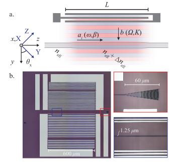
Figure 1: SAW Phase Modulator. a. Aluminum IDTs generate surface waves in the LN film on sapphire which travel normal to an optical ridge waveguide. These surfaces waves modulate the effective index of the optical modes in the waveguide. b. Pictures of the fabricated device showing the IDTs, ridge waveguide, and focusing grating couplers.

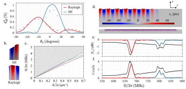
Figure 2: Piezoelectric response. a. We compute the piezoelectric coupling coefficient $k_{\textrm{eff}}^{2}$ from the X-point solutions for a unit cell of the IDT (b.). The Rayleigh wave (red) and SH wave (blue) exhibit $k_{\textrm{eff}}^{2}$ on the order of $1\%$. Measurements of $k_{\textrm{eff}}^{2}$ (points) are overlaid on the simulated curves. c. Bands for the slab (no electrodes) with $\theta_{\textrm{x}}=0^{\circ}$ show the Rayleigh mode (red) is guided, i.e. below the sound cone in sapphire (hatched), for all frequencies. At $2.7\text{\,}\mathrm{GHz}$, the SH mode (blue) emerges from the sound cone, but even below this frequency, the radiation-limited propagation length is long enough to use the mode for modulation. d. The conductance is computed for a thin cross-section of the transducer. The $S_{11}$, e., and conductance $G$, f., are plotted for measurements (black) and simulations (red-blue gradient colored by mode).

The surface waves generated by the IDT strain and deform the optical waveguides. This changes the effective index $n_{\textrm{eff}}$ of the fundamental TE-like optical mode as captured by the optomechanical coupling coefficient $g$. The coupling coefficient is computed from the optical and piezoelectric eigenmodes of an extruded cross-section of the waveguide solved for by FEM in COMSOL COM to capture the full vectorial nature of the fields. The optical mode propagates into the plane in Figure 4a and the piezoelectric mode across the plane in Figure 4b. The electric field of the TE-like optical mode is antisymmetric with respect to the $xz$ symmetry plane. At each $\theta_{\textrm{x}}$, these solutions are used to evaluate $g$ by the perturbative overlap integral (detailed in Appendix A)

$$g=-\frac{\omega}{\mathcal{P}_{1}}\int\textrm{d}A\mathbf{E}^{*}_{1}\delta_{u}\varepsilon\cdot\mathbf{u}_{0}\mathbf{E}_{0}.$$ (3)

$\mathbf{E}_{j}$ and $\mathbf{u}_{k}$ are the electromagnetic and displacement field distributions for the guided mode solutions, $\omega$ is the optical frequency, $\mathcal{P}_{j}$ is the time-averaged optical power, and $\delta_{u}\varepsilon$ is the modification of the structure’s dielectric constant distribution due to motion, which includes both the shifts in the boundaries and the contribution of the photoelastic tensor.

Despite the nontrivial dependence of $g$ on waveguide orientation as plotted in Figure 4, a simple picture describes the interaction at the peaks. Consider the Rayleigh and fundamental TE modes. The $S_{yy}$ component of the strain — the dominant component of the Rayleigh waves at the surface — modulates the $\varepsilon_{yy}$ component of the permittivity via the $p_{yyyy}$ component of the photoelastic tensor. Modulating $\varepsilon_{yy}$ modulates the TE mode which has a $y$-oriented electric field. In Figure 4c, the coupling coefficient peaks at $\theta_{\textrm{x}}=-45^{\circ}$ where $p_{yyyy}$ reaches a maximum of $0.30$ for X-cut LN. Similarly, interactions with the SH mode are dominated by $p_{yyyz}$ which has local extrema of $0.127$ and $-0.135$ at $\theta_{\textrm{x}}=-18^{\circ}$ and $32^{\circ}$, respectively.

II Fabrication and characterization

We start our process with $5\times$10\text{\,}\mathrm{mm}$$ chips of $525\text{\,}\mathrm{nm}$-thick LN-on-sapphire. The LN is X-cut and the c-axis of the sapphire is normal to the wafer. The a-axis of the sapphire and the Z-axis of the LN are in-plane and parallel. Ridge waveguides and grating couplers are patterned into a hydrogen silsesquioxane (HSQ) mask and transferred to the sample by a $300\text{\,}\mathrm{nm}$ argon ion etch leaving a $225\text{\,}\mathrm{nm}$ thick LN slab on the sapphire substrate. The remaining mask is stripped with hydrofluoric acid before the chip is cleaned with piranha. The $200\text{\,}\mathrm{nm}$ thick aluminum electrodes are patterned by lift-off on the $225\text{\,}\mathrm{nm}$ LN slab. The IDT is $600\text{\,}\mathrm{\SIUnitSymbolMicro m}$ wide and has $30$ aluminum finger-pairs. The ridge waveguide is $1.25\text{\,}\mathrm{\SIUnitSymbolMicro m}$ wide and supports a TE-like and a TM-like optical mode.

Below we describe how $k_{\textrm{eff}}$ and $g$ are extracted from measurements of the IDTs’ linear response and the modulators’ modulation index.

II.1 Piezoelectric coupling coefficient in LN-on-sapphire

In order to characterize the piezoelectric quality of the film, we measure the coupling coefficient $k_{\textrm{eff}}^{2}$ and compare it to simulations. The coupling coefficient is extracted from measurements of the one-port microwave response $S_{11}$ of the IDT for a range of crystal orientations $\theta_{\textrm{x}}$ varying from $-90^{\circ}$ to $90^{\circ}$.

We measure the S-parameter of each device on a calibrated probe station (GGB 40-A nickel probes) with an R&S ZNB20 vector network analyzer (Figure 2e) to determine the admittance $Y\left(\omega\right)$. The coupling can be computed directly from the measured conductance $G(\omega)~{}\equiv~{}\textrm{Re}Y(\omega)$ Dahmani et al. (2019)

$$k_{\textrm{eff}}^{2}=\frac{\pi\int\textrm{d}\omega G\left(\omega\right)}{4C_{0}\Omega_{0}^{2}}$$ (4)

where $C_{0}$ is the static capacitance computed by fit to the susceptance $-\textrm{Im}Y(\omega)$ near DC, $\Omega_{0}$ is the center frequency of the response, and the integral is evaluated about $\Omega_{0}$. In addition to the mechanical signature (red-blue curve in Figure 2f), $G(\omega)$ is offset by a slowly increasing background which comes from ohmic loss and inductance of the IDT. This effect is not captured in the cross-section modeled in Section I which assumes the fields are uniform along the fingers. We fit the background to a parabola and remove it from $G$ before computing $k_{\textrm{eff}}^{2}$ by Equation 4. This gives us the points in Figure 2a.

We find excellent agreement between the shape of the simulated and measured $k_{\textrm{eff}}^{2}(\theta_{\textrm{x}})$ as shown in Figure 2a. The magnitude of the Rayleigh response matches with simulation, but the SH response falls 20% below the simulated response at its peak near $0^{\circ}$. A reduction of around $10\%$ in the piezoelectric tensor component $d_{\textrm{YZY}}$ from $69$ to $62\text{\,}\mathrm{pC}\text{\,}{\mathrm{N}}^{-1}$ would lead to this reduction in $k_{\textrm{eff}}^{2}$.

An important advantage of the LN-on-sapphire platform is that horizontal shear (SH) waves are strongly piezoelectric at high frequency. To demonstrate this, we repeat the above procedure for $2\text{\,}\mathrm{\SIUnitSymbolMicro m}$-pitch IDTs on $200\text{\,}\mathrm{nm}$-thick LN-on-sapphire. A typical conductance curve is shown in Figure 3a for $\theta_{\textrm{x}}=0^{\circ}$. For these $15$-finger-pair, $50\text{\,}\mathrm{\SIUnitSymbolMicro m}$-wide transducers, the proximity of the Rayleigh and SH waves makes it difficult to independently filter their contributions to $G$. Instead we integrate the conductance for the blue shaded region (between $1$ and $2.65\text{\,}\mathrm{GHz}$) and report the sum of $k_{\textrm{eff}}^{2}$ for both modes (Figure 3b). Simulations show that the Rayleigh mode remains weakly coupled, and so the increase in $k_{\textrm{eff}}^{2}$ is primarily due to the SH mode. The results of measurements of IDTs at a variety of angles are plotted in Figure 3, showing that $k_{\textrm{eff}}^{2}$ for the SH mode exceeds $10\%$.

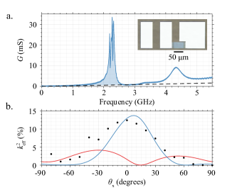
Figure 3: High $k_{\textrm{eff}}^{2}$ mechanics. At higher frequencies, the coupling coefficient of the SH mode exceeds $10\%$. a. The conductance of $2\text{\,}\mathrm{\SIUnitSymbolMicro m}$-pitch IDTs can be integrated near the Rayleigh and SH response just above $2\text{\,}\mathrm{GHz}$ to calculate the sum of $k_{\textrm{eff}}^{2}$ for the two modes. A linear background (dashed) is removed from $G$. An example device is inset. b. Measurements of the summed $k_{\textrm{eff}}^{2}$ (black dots) are plotted against simulations of the coupling of Rayleigh (red) and SH (blue) mode.

II.2 Optomechanics in LN-on-sapphire

We investigate the optomechanical properties of the bonded LN film — in particular, the photoelastic coefficients — by measuring the optomechanical coupling coefficient $g$ of a nanophotonic ridge waveguide and comparing it to simulations. As with $k_{\textrm{eff}}^{2}$, $g$ varies with crystal orientation because LN is strongly anisotropic.

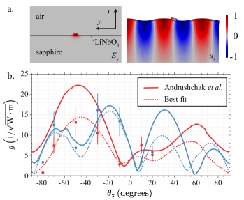
Figure 4: Optomechanical response. a. The effective index of the TE optical mode (left) is modulated by the Rayleigh wave (right). b. Angular dependence of the simulated (solid, photoelastic tensor from Ref. Andrushchak et al. (2009)) and measured (dots) optomechanical coupling coefficient. Simulations of $g$ with best fit photoelastic coefficients are plotted (dashed). Red and blue are Rayleigh and SH modes as before.

We determine $g$ by sending light through the device while driving the IDT with a microwave signal, and measuring the modulation index $h_{\textrm{oa}}$ of the transmitted light. The IDT transmission $t_{\textrm{b}\upmu}$ is used in this calibration to determine the mechanical power incident on the waveguide due to the microwave driving. We measure the modulation index with the apparatus diagrammed in Figure 5a which is used to detect the resulting phase modulation. We tune a C-band laser (Santec TSL-550) to the edge of a Teraxion fiber Bragg notch filter near $1551$ nm such that phase modulation by the device is converted to intensity modulation. This intensity modulated light is then amplified (FiberPrime EDFA-C-26G-S) and detected on a photodiode (Optilab PD-40-M). We drive the modulator and read out the photocurrent fluctuations on a vector network analyzer (VNA, R&S ZNB20). The modulation index $h_{\textrm{oa}}$ is calibrated by comparing the acousto-optic signal to phase modulation from an electro-optic modulator (EOM) cascaded with the device

$$h_{\textrm{oa}}=h_{\textrm{oe}}\left|\frac{S_{\textrm{oa}}}{S_{\textrm{oe}}}\right|.$$ (5)

Here $S_{\textrm{oa}}$ and $S_{\textrm{oe}}$ are S-parameters measured on the VNA for an acousto-optic device and the EOM, respectively, at the peak acousto-optic response. The EOM is calibrated independently using a tunable Fabry-Pérot filter (Micron Optics FFP-TF) to filter and measure the power of the pump and sidebands for a given RF drive power $P$.

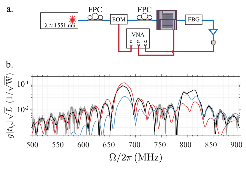
Figure 5: Acousto-optic measurements. a. Apparatus used to measure the modulation index. b. Measurements of the modulation efficiency $h_{\textrm{ao}}/2\sqrt{P}$ in gray are overlaid with predictions $gt_{\textrm{b}\upmu}\sqrt{L}$ from FEM simulations of the Rayleigh (red) and SH (blue) modes for $\theta_{\textrm{x}}=-30^{\circ}$. The black curve is filtered in the time-domain to eliminate contributions from reflections.

The modulation index $h_{\textrm{oa}}$ is not a direct measurement of the coupling coefficient. Instead the measured quantity plotted in Figure 5b

$$\frac{h_{\textrm{oa}}}{2\sqrt{P}}=g\left|t_{\textrm{b}\upmu}\right|\sqrt{L}$$ (6)

is the product of $g$, the square root of the efficiency of the IDT $\left|t_{\textrm{b}\upmu}\right|$, and the square root of the length of the interaction region $L$. The numerical values for $g|t_{\textrm{b}\upmu}|$ are overlaid on the measurements in Figure 5b for the Rayleigh (red) and SH (blue) mode.

For the measured coupling coefficients in Figure 4b, we extract the peaks of $h_{\textrm{oa}}$ for each mode and remove a factor of $|t_{\textrm{b}\upmu}|$ determined numerically. The accuracy of the resulting rates are susceptible to errors in $t_{\textrm{b}\upmu}$. In Dahmani et al. where the transmission coefficient was de-embedded directly from measurements, the simulated $t_{\textrm{b}\upmu}$ of 8.9% was larger than the measured 7.0% by $27\%$ Dahmani et al. (2019). If we overestimate $t_{\textrm{b}\upmu}$, we will underestimate $g$ and therefore the photoelastic coefficients. On the other hand, reflections, e.g. off the waveguide, can give rise to standing waves which can enhance the IDT’s efficiency. A fractional uncertainty of 27% like that in Dahmani et al. (plotted in Figure 4b) would not account for the deviation from theory using bulk material properties. We perform a regression on $g(\theta_{\textrm{x}})$ in Appendix B to estimate the photoelastic tensor had the deviation been only due to a discrepancy between bulk and our thin-film’s $p_{ij}$. We find that scaling $p_{33},p_{44},$ and $p_{41}$ by factors of 32%, 70%, and 35%, respectively, gives the best fit dashed curve in Figure 4b.

III Conclusion

Lithium niobate-on-sapphire has many bright prospects in optics and, specifically, in acousto-optics. In this platform, the piezoelectric LN film supports both Rayleigh and horizontal shear surface waves which can be generated with interdigital transducers and used to modulate optical waveguides patterned in LN. Here we measure the piezoelectric coupling coefficients of transducers and optomechanical coupling coefficients of ridge waveguides for a range of crystal orientations in X-cut LN, confirming the quality of these bonded films and demonstrating the potential of the material platform.

As the mechanical frequency reaches into the GHz regime, $k_{\textrm{eff}}^{2}$ of the horiztonal shear waves exceeds 10%, making it possible to make compact, broadband transducers. Future work in pursuit of low-power acousto-optic devices calls for the efficient, mode-selective transduction of wavelength-scale waveguides. Waveguide transducers like those recently developed for horizontal shear waves in suspended LN films can enable a new generation of ultra-low-power phononic devices and acousto-optic modulators Dahmani et al. (2019). As the array of electro-optic and nonlinear optical devices in thin-film LN grows, so too grow the prospects for integrating acousto-optic devices into complex phononic and photonic circuits and systems built on these rapidly developing platforms.

Appendix A Optomechanics of side-coupled waveguides

For intuition we adopt a quasi-static picture of the dynamics, treating the mechanical waves as stationary relative to light traveling along the waveguide. At time $t$, the mechanical wave deforms the waveguide uniformly along its length $z$. This deformation $\mathbf{u}\left(t,x,y\right)=\mathbf{u}_{0}\left(x,y\right)\cos\Omega t$ of the waveguide’s cross-section (radiation pressure) and the associated strain-induced change in the index (photoelastic effect) Andrushchak et al. (2009) vary the permittivity, which to first order in $\mathbf{u}$,

$$\Delta\varepsilon =\delta_{\mathbf{u}}\varepsilon\cdot\mathbf{u}\left(t,x,y\right)$$ (7a)

$$=\delta_{\partial\Omega}\left(\Delta\varepsilon\Pi_{\perp}-\varepsilon\Delta\varepsilon^{-1}\Pi_{\shortparallel}\varepsilon\right)\mathbf{u}\cdot\hat{n}-\varepsilon\frac{p\mathbf{S}}{\varepsilon_{0}}\varepsilon,$$ (7b)

shifts the wavevector of the guided optical wave $\Delta\beta\cos\Omega t.$ Here $\delta_{\partial\Omega}$ is a delta function zero everywhere except dielectric boundaries, $p$ is the photoelastic tensor, and $S$ is the strain. The projectors $\Pi_{\perp}$ and $\Pi_{\shortparallel}$ project out the field perpendicular and parallel to the normal $\hat{n}$, respectively. In this manner, the phase of light leaving the waveguide is acousto-optically modulated

$$a\left(t,z=L\right)=a\left(0,L\right)e^{i\Delta\beta L\cos\Omega t}.$$ (8)

The phase modulation index $h_{\textrm{oa}}\equiv\Delta\beta L$ is related to the optomechanical coupling $g$ familiar in stimulated Brillouin scattering. By adopting a power-orthogonal basis for the electric field $\mathbf{E}=\Sigma_{n}\mathbf{E}_{n}a_{n}e^{-i\left(\omega+n\Omega\right)t}$, the interaction can be expressed in terms of coupled-modes Yariv (1973); Wolff et al. (2015). For short lengths and low RF drive powers, the $n=+1$ mode evolves as

$$\left(\partial_{z}+v_{\textrm{g}}^{-1}\partial_{t}\right)a_{1}\left(t,z\right)=igba_{0}$$ (9)

where $b$ is the amplitude of the mechanics $\mathbf{u}=\mathbf{u}_{0}be^{-i\Omega t}$. The optomechanical coupling can be expressed in terms of the mode profiles

$$g=-\frac{\omega}{\mathcal{P}_{1}}\int\textrm{d}A\mathbf{E}^{*}_{1}\delta_{u}\varepsilon\cdot\mathbf{u}_{0}\mathbf{E}_{0}$$ (10)

where $\mathcal{P}_{i}$ is the time-averaged optical power into the waveguide for mode $i$. If we use a power-orthonormal basis for the optics such that $\left|a_{i}\right|^{2}$ is the power in mode $i$, $\mathcal{P}_{i}$ becomes $1$ for all $i$ and Eq. 10 takes on a more symmetric form for various mode pairs.

We have yet to choose a normalization for the displacement $\mathbf{u}_{0}$ and thereby units for both $g$ and $b$. For the devices described here, the devices in Sohn et al. Sohn, Kim, and Bahl (2018), and work on AO-modulated Mach-Zehnder interferometers Poveda et al. (2019); Cai et al. (2019); Khan et al. (2019), the mechanical wave propagates across the waveguide. In this configuration, the displacement of the waveguide scales as the square root of the mechanical power density, which is the power per unit length along the waveguide. A $1\text{\,}\mathrm{mW}$ wave generated by a $100\text{\,}\mathrm{\SIUnitSymbolMicro m}$-wide IDT will deform the waveguide the same as that of a $2\text{\,}\mathrm{mW}$ wave from a $200\text{\,}\mathrm{\SIUnitSymbolMicro m}$-wide IDT. We normalize the displacement field $\mathbf{u}_{0}$ such that $b^{2}$ is the mechanical power density with units of $$\mathrm{W}$/$\mathrm{m}$$. Therefore the coupling coefficient $g$ has units of $1/\sqrt{$\mathrm{W}$\cdot$\mathrm{m}\mathrm{e}\mathrm{t}\mathrm{e}\mathrm{r}$}$.

Finally, when $gb\ll L$, we can integrate Equation 9 and compare it to equation Equation 8 to find

$$\frac{h_{\textrm{oa}}}{2} =gbL$$ (11a)

$$=g\sqrt{P_{\textrm{m}}L}.$$ (11b)

Substituting in the efficiency of the IDT, $P_{\textrm{m}}=\left|t_{\textrm{b}\upmu}\right|^{2}P$ where $P$ is the RF power incident on the IDT, we arrive at Equation 6.

It may be surprising that the modulator’s efficiency $h_{\textrm{oa}}^{2}/4P$ — the sideband power ratio divided by the RF drive power, which is the square of the expression in Equation 6 — scales as $L$ and not $L^{2}$, but this scaling is essentially the same as in electro-optic modulation. A typical electro-optic modulator is nearly identical to the optomechanical modulator described here except that instead of applying a displacement $\mathbf{u}$ in Equation 7b to change the permittivity of a waveguide, a voltage is applied to a capacitor to shift the effective index $\Delta n_{\textrm{eff}}$ by the electro-optic effect. The phase shift of light transmitted through the waveguide $\Delta n_{\textrm{eff}}L$ is proportional to $L$, and therefore the power in the sidebands is proportional to $L^{2}$. But just as the total mechanical power $P_{\textrm{m}}$ scales as $L$, the energy in a capacitor along the waveguide scales as $L$. The result is that, like the optomechanical modulator described here, the efficiency of an electro-optic modulator scales as $L$.

Equation 10 is used to compute the $g$ plotted in Figure 4 of the main text. In our calculation we model the photoelastic effect in sapphire using coefficients measured in ruby Waxler and Farabaugh (1970) and, for the radiation pressure term, LN is treated as an isotropic medium with refractive index of $2.15$.

Finally, our device is at heart an electrically-driven analog of the optomechanical waveguides investigated in the field of guided-wave Brillouin scattering. In those systems Shin et al. (2013); Van Laer et al. (2015); Wiederhecker, Dainese, and Mayer Alegre (2019); Eggleton et al. (2019); Safavi-Naeini et al. (2019) the mechanical motion is typically driven optically, while here the mechanical motion is driven electrically. The optomechanical coupling coefficient $g$ used here (Equation 10) is, up to a few conversion factors, identical in nature to the Brillouin gain coefficient $\mathcal{G}_{\text{B}}$ and the refractive-index sensitivity to mechanical motion $\partial_{x}n_{\text{eff}}$. The explicit connection is as follows. The modulation index can be written as

$$\frac{h_{\textrm{oa}}}{2}=gbL=\frac{\Delta\beta L}{2}=k_{0}\partial_{x}n_{\text{eff}}Lx$$ (12)

with $k_{0}$ the free-space optical wavevector and $x$ a coordinate representing the mechanical motion. From previous work Van Laer et al. (2015); Van Laer, Baets, and Van Thourhout (2016) we have

$$\partial_{x}n_{\text{eff}}=c\sqrt{\frac{\mathcal{G}_{\text{B}}\omega_{\text{m}}^{2}m_{\text{eff}}}{2\omega_{0}Q_{\text{m}}}}$$ (13)

with $c$ the speed of light, $\omega_{0}$ the optical frequency, $Q_{\text{m}}$ the mechanical quality factor, $\omega_{\text{m}}$ the mechanical frequency, $m_{\text{eff}}=\int\textrm{d}A\rho|\mathbf{u}|^{2}$ the effective mechanical mode mass, and $\rho$ the mass density. This shows that the optomechanical coupling coefficient $g$ used here and the Brillouin gain coefficient are rigorously connected. We note that the optomechanical coupling coefficient $g\propto\sqrt{\mathcal{G}_{\text{B}}}$ scales as the square root of the Brillouin gain coefficient, since the latter takes into account both optical driving and optical read-out of the mechanics, whereas in this work only the read-out of the mechanics occurs optically.

Appendix B Regressing the photoelastic coefficients

Our measurements of $g$ in Figure 4 show rough agreement with the coupling predicted using values of the photoelastic tensor of bulk LN measured by Andrushchak et al. Andrushchak et al. (2009). We would like to go beyond this qualitative comparison and find the components $p_{ij}$ that best fit the data. There are $d=8$ distinct components of $p$ for LN, with the remaining components constrained by the symmetry of the crystal lattice. In order to avoid overfitting our $n=14$ measurements — 2 modes, Rayleigh and SH, measured at 7 angles $\theta_{\textrm{x}}$, each — we start with a regularized fit before reducing the regression to just three components of $p$.

In Appendix A, we outline how the photoelastic tensor $p$ is related to the coupling coefficient $g$. Since $g$ is proportional to $\delta\varepsilon_{u}$ and $\delta\varepsilon_{u}$ is linearly dependent on $p$, the coupling is a linear function of $p$ which can be expressed

$$g=\left|Ap+b\right|$$ (14)

In Equation 14, $g\in\mathbb{R}^{n}$, $p\in\mathbb{R}^{d}$, $A\in\mathbb{C}^{n\times d}$, and $b\in\mathbb{C}^{n}$. Both $A$ and $b$ are computed as described in the main text. They are complex because $u$, the mechanical field, is complex. The phase of $u$ can be chosen to make $g$ real but this in turn affects the phase of $t_{\textrm{b}\upmu}$. Although the phase of $gt_{\textrm{b}\upmu}$ does factor into the phase of $S_{\textrm{ao}}$, we restrict our measurements to the magnitude of $gt_{\textrm{b}\upmu}$.

We start by solving

$$\min_{p}\left\|\left|Ap+b\right|-g\right\|+\lambda\left\|p-p_{0}\right\|_{1}$$ (15)

where $\left\|\cdot\right\|_{1}$ is the L¹ norm. The second term in Equation 15 is used to regularize the fit. It penalizes deviation from $p_{0}$, the values measured for bulk LN by Andrushchak et al.. Using an L¹ norm encourages $p-p_{0}$ to be sparse. As $\lambda$ is increased, some components of $p-p_{0}$ fix to $0$. At first, the quality of the fit (the first term in the right-hand side of Equation 15) is relatively unaffected by the reduction of dimension $d$. Ultimately the regularization term begins to exert a pressure on the components of $p$ needed to fit the data and the fit diverges from the measured values. At this point we are left with just three components of $p$ which deviate from $p_{0}$ : $p_{33}$, $p_{44}$, and $p_{41}$ in Voigt notation.

	Andrushchak et al. Andrushchak et al. (2009)	Fit
$p_{11}$	$-0.021\pm 0.018$	—
$p_{12}$	$0.060\pm 0.019$	—
$p_{13}$	$0.172\pm 0.029$	—
$p_{31}$	$0.141\pm 0.017$	—
$p_{33}$	$0.118\pm 0.020$	0.038
$p_{14}$	$-0.052\pm 0.007$	—
$p_{41}$	$-0.109\pm 0.017$	-0.038
$p_{44}$	$0.121\pm 0.019$	0.085

Table 1: Photoelastic coefficients for bulk LN and the best fit from the $g$ measurements in Figure 4.

We repeat the regression setting $\lambda$ to 0 and removing all other components of $p$ from the fit to find the values in Table 1 giving us the dashed curves in Figure 4b.

References

- Wang et al. (2014) C. Wang, M. J. Burek, Z. Lin, H. A. Atikian, V. Venkataraman, I.-C. Huang, P. Stark, and M. Lončar, “Integrated high quality factor lithium niobate microdisk resonators,” Optics express 22, 30924–30933 (2014).
- Levy et al. (1998) M. Levy, R. Osgood Jr, R. Liu, L. Cross, G. Cargill III, A. Kumar, and H. Bakhru, “Fabrication of single-crystal lithium niobate films by crystal ion slicing,” Applied Physics Letters 73, 2293–2295 (1998).
- Yu et al. (2019) M. Yu, C. Wang, M. Zhang, and M. Loncar, “Chip-based lithium-niobate frequency combs,” IEEE Photonics Technology Letters (2019).
- Rao et al. (2016a) A. Rao, M. Malinowski, A. Honardoost, J. R. Talukder, P. Rabiei, P. Delfyett, and S. Fathpour, “Second-harmonic generation in periodically-poled thin film lithium niobate wafer-bonded on silicon,” Optics express 24, 29941–29947 (2016a).
- Chang et al. (2016) L. Chang, Y. Li, N. Volet, L. Wang, J. Peters, and J. E. Bowers, “Thin film wavelength converters for photonic integrated circuits,” Optica 3, 531–535 (2016).
- Rao et al. (2016b) A. Rao, A. Patil, P. Rabiei, A. Honardoost, R. DeSalvo, A. Paolella, and S. Fathpour, “High-performance and linear thin-film lithium niobate mach–zehnder modulators on silicon up to 50 ghz,” Optics letters 41, 5700–5703 (2016b).
- Wang et al. (2018) C. Wang, M. Zhang, B. Stern, M. Lipson, and M. Lončar, “Nanophotonic lithium niobate electro-optic modulators,” Optics express 26, 1547–1555 (2018).
- Olsson III et al. (2014) R. H. Olsson III, K. Hattar, S. J. Homeijer, M. Wiwi, M. Eichenfield, D. W. Branch, M. S. Baker, J. Nguyen, B. Clark, T. Bauer, and T. A. Friedmann, “A high electromechanical coupling coefficient sh0 lamb wave lithium niobate micromechanical resonator and a method for fabrication,” Sensors and Actuators A: Physical 209, 183–190 (2014).
- Pop et al. (2017) F. V. Pop, A. S. Kochhar, G. Vidal-Alvarez, and G. Piazza, “Laterally vibrating lithium niobate mems resonators with 30% electromechanical coupling coefficient,” in 2017 IEEE 30th International Conference on Micro Electro Mechanical Systems (MEMS) (IEEE, 2017) pp. 966–969.
- Manzaneque et al. (2019) T. Manzaneque, R. Lu, Y. Yang, and S. Gong, “Low-loss and wideband acoustic delay lines,” IEEE Transactions on Microwave Theory and Techniques 67, 1379–1391 (2019).
- Dahmani et al. (2019) Y. D. Dahmani, C. J. Sarabalis, W. Jiang, F. M. Mayor, and A. H. Safavi-Naeini, “Piezoelectric transduction of a wavelength-scale mechanical waveguide,” arXiv preprint arXiv:1907.13058 (2019).
- Shao et al. (2019) L. Shao, M. Yu, S. Maity, N. Sinclair, L. Zheng, C. Chia, A. Shams-Ansari, C. Wang, M. Zhang, K. Lai, and M. Lončar, “Microwave-to-optical conversion using lithium niobate thin-film acoustic resonators,” Optica 6, 1498–1505 (2019).
- Jiang et al. (2020) W. Jiang, C. J. Sarabalis, Y. D. Dahmani, R. N. Patel, F. M. Mayor, T. P. McKenna, R. Van Laer, and A. H. Safavi-Naeini, “Efficient bidirectional piezo-optomechanical transduction between microwave and optical frequency,” Nature Communications 11, 1–7 (2020).
- Tadesse and Li (2014) S. A. Tadesse and M. Li, “Sub-optical wavelength acoustic wave modulation of integrated photonic resonators at microwave frequencies,” Nature Communications 5, 5402 (2014).
- Kittlaus et al. (2020) E. A. Kittlaus, W. M. Jones, P. T. Rakich, N. T. Otterstrom, R. E. Muller, and M. Rais-Zadeh, “Electrically-driven acousto-optics and broadband non-reciprocity in silicon photonics,” arXiv preprint arXiv:2004.01270 (2020).
- van der Poel et al. (2007) M. van der Poel, M. Beck, M. B. Dühring, M. M. de Lima, L. H. Frandsen, C. Peucheret, O. Sigmund, U. Jahn, J. M. Hvam, and P. Santos, “Surface acoustic wave driven light modulation,” in Proceedings of 13th European Conference on Integrated Optics (Citeseer, 2007) p. FB3.
- Van Der Slot, Porcel, and Boller (2019) P. J. Van Der Slot, M. A. Porcel, and K.-J. Boller, “Surface acoustic waves for acousto-optic modulation in buried silicon nitride waveguides,” Optics express 27, 1433–1452 (2019).
- Cai et al. (2019) L. Cai, A. Mahmoud, M. Khan, M. Mahmoud, T. Mukherjee, J. Bain, and G. Piazza, “Acousto-optical modulation of thin film lithium niobate waveguide devices,” Photonics Research 7, 1003–1013 (2019).
- Mahmoud et al. (2018a) M. Mahmoud, A. Mahmoud, L. Cai, M. Khan, T. Mukherjee, J. Bain, and G. Piazza, “Novel on chip rotation detection based on the acousto-optic effect in surface acoustic wave gyroscopes,” Optics express 26, 25060–25075 (2018a).
- Mahmoud et al. (2018b) A. Mahmoud, M. Mahmoud, L. Cai, M. Khan, J. A. Bain, T. Mukherjee, and G. Piazza, “Acousto-optic gyroscope,” in 2018 IEEE Micro Electro Mechanical Systems (MEMS) (IEEE, 2018) pp. 241–244.
- Crespo-Poveda et al. (2015) A. Crespo-Poveda, A. Hernández-Mínguez, B. Gargallo, K. Biermann, A. Tahraoui, P. Santos, P. Muñoz, A. Cantarero, and M. de Lima, “Acoustically driven arrayed waveguide grating,” Optics express 23, 21213–21231 (2015).
- Crespo-Poveda et al. (2016) A. Crespo-Poveda, A. Hernández-Mínguez, K. Biermann, A. Tahraoui, B. Gargallo, P. Muñoz, P. V. Santos, A. Cantarero, and M. M. de Lima Jr, “Tunable arrayed waveguide grating driven by surface acoustic waves,” in Smart Photonic and Optoelectronic Integrated Circuits XVIII, Vol. 9751 (International Society for Optics and Photonics, 2016) p. 97510Y.
- Khan et al. (2019) M. Khan, A. Mahmoud, L. Cai, M. Mahmoud, T. Mukherjee, J. A. Bain, and G. Piazza, “Extraction of elasto-optic coefficient of thin film arsenic trisulfide using a mach-zehnder acousto-optic modulator on lithium niobate,” Journal of Lightwave Technology (2019).
- Hashimoto and Hashimoto (2000) K.-y. Hashimoto and K.-Y. Hashimoto, Surface acoustic wave devices in telecommunications (Springer, 2000).
- Hashimoto (2009) K.-y. Hashimoto, RF bulk acoustic wave filters for communications (Artech House, 2009).
- Andrushchak et al. (2009) A. Andrushchak, B. Mytsyk, H. Laba, O. Yurkevych, I. Solskii, A. Kityk, and B. Sahraoui, “Complete sets of elastic constants and photoelastic coefficients of pure and mgo-doped lithium niobate crystals at room temperature,” Journal of Applied Physics 106, 073510 (2009).
- Auld (1990) B. A. Auld, Acoustic fields and waves in solids, Volume II, 2nd ed. (Robert E. Krieger Publishing Company, Malabar, Florida, 1990).
- (28) COMSOL Multiphysics® v. 5.4, COMSOL AB, Stockholm, Sweden.
- Yariv (1973) A. Yariv, “Coupled-mode theory for guided-wave optics,” IEEE Journal of Quantum Electronics 9, 919–933 (1973).
- Wolff et al. (2015) C. Wolff, M. J. Steel, B. J. Eggleton, and C. G. Poulton, “Stimulated brillouin scattering in integrated photonic waveguides: Forces, scattering mechanisms, and coupled-mode analysis,” Physical Review A 92, 013836 (2015).
- Sohn, Kim, and Bahl (2018) D. B. Sohn, S. Kim, and G. Bahl, “Time-reversal symmetry breaking with acoustic pumping of nanophotonic circuits,” Nature Photonics 12, 91 (2018).
- Poveda et al. (2019) A. C. Poveda, D. D. Bühler, A. C. Sáez, P. V. Santos, and M. M. de Lima Jr, “Semiconductor optical waveguide devices modulated by surface acoustic waves,” Journal of Physics D: Applied Physics 52, 253001 (2019).
- Waxler and Farabaugh (1970) R. Waxler and E. Farabaugh, “Photoelastic constants of ruby,” J. Res. Nat. Bur. Stand. 74, 215–220 (1970).
- Shin et al. (2013) H. Shin, W. Qiu, R. Jarecki, J. Cox, R. Olsson, A. Starbuck, Z. Wang, and P. Rakich, “Tailorable stimulated Brillouin scattering in nanoscale silicon waveguides,” Nature Communications 4, 1944 (2013).
- Van Laer et al. (2015) R. Van Laer, B. Kuyken, D. Van Thourhout, and R. Baets, “Interaction between light and highly confined hypersound in a silicon photonic nanowire,” Nature Photonics 9, 199–203 (2015), arXiv:1407.4977 .
- Wiederhecker, Dainese, and Mayer Alegre (2019) G. S. Wiederhecker, P. Dainese, and T. P. Mayer Alegre, “Brillouin optomechanics in nanophotonic structures,” APL Photonics 4, 071101 (2019).
- Eggleton et al. (2019) B. J. Eggleton, C. G. Poulton, P. T. Rakich, M. J. Steel, and G. Bahl, “Brillouin integrated photonics,” Nature Photonics 13, 664–677 (2019).
- Safavi-Naeini et al. (2019) A. H. Safavi-Naeini, D. Van Thourhout, R. Baets, and R. Van Laer, “Controlling phonons and photons at the wavelength scale: integrated photonics meets integrated phononics,” Optica 6, 213 (2019).
- Van Laer, Baets, and Van Thourhout (2016) R. Van Laer, R. Baets, and D. Van Thourhout, “Unifying Brillouin scattering and cavity optomechanics,” Physical Review A 93, 15 (2016), arXiv:1503.03044 .