Sl-EDGE: Network Slicing at the Edge

Abstract.

Network slicing of multi-access edge computing (MEC) resources is expected to be a pivotal technology to the success of 5G networks and beyond. The key challenge that sets MEC slicing apart from traditional resource allocation problems is that edge nodes depend on tightly-intertwined and strictly-constrained networking, computation and storage resources. Therefore, instantiating MEC slices without incurring in resource over-provisioning is hardly addressable with existing slicing algorithms. The main innovation of this paper is Sl-EDGE, a unified MEC slicing framework that allows network operators to instantiate heterogeneous slice services (e.g., video streaming, caching, 5G network access) on edge devices. We first describe the architecture and operations of Sl-EDGE, and then show that the problem of optimally instantiating joint network-MEC slices is NP-hard. Thus, we propose near-optimal algorithms that leverage key similarities among edge nodes and resource virtualization to instantiate heterogeneous slices $7.5$x faster and within $0.25$ of the optimum. We first assess the performance of our algorithms through extensive numerical analysis, and show that Sl-EDGE instantiates slices 6x more efficiently then state-of-the-art MEC slicing algorithms. Furthermore, experimental results on a 24-radio testbed with 9 smartphones demonstrate that Sl-EDGE provides at once highly-efficient slicing of joint LTE connectivity, video streaming over WiFi, and ffmpeg video transcoding.

1. Introduction

It is now clear that advanced softwarization and virtualization paradigms such as network slicing will be the cornerstone of 5G networks (D’Oro et al., 2020) and the Internet of Things (Bizanis and Kuipers, 2016). Indeed, by sharing a common underlying physical infrastructure, network operators (NOs) can dynamically deploy multiple “slices” tailored for specific services (e.g., video streaming, augmented reality), as well as requirements (e.g., low latency, high throughput, low jitter) (ETSI, 2018a), avoiding the static—thus, inefficient—network deployments that have plagued traditional hardware-based cellular networks. To further decrease latency, increase throughput, and provide improved services to their subscribers, NOs have recently started integrating multi-access edge computing (MEC) technologies (Taleb et al., 2017), which are expected to become essential to reach the sub-1 ms latency requirements of 5G. MEC will be so quintessential that the European Telecommunications Standards Institute (ETSI) has identified MEC as “one of the key pillars for meeting the demanding Key Performance Indicators (KPIs) of 5G” and “[as playing] an essential role in the transformation of the telecommunications business” (ETSI, 2018b).

Despite the clear advantages of network slicing and MEC, the truth of the matter is that we cannot have one without the other. Indeed, slicing networking resources only, e.g., spectrum and resource blocks (RBs) cannot suffice to satisfy the stringent timing and performance requirements of 5G networks. Real-time wireless video streaming, for example, requires at the same time (i) networking resources (e.g., RBs) to broadcast the video, (ii) computational resources to process and transcode the video, as well as (iii) storage resources to locally cache the video. The key issue that sets MEC slicing apart from traditional slicing problems is that MEC resources are usually coupled, meaning that slicing one resource usually leads to a performance degradation in another type of resource.

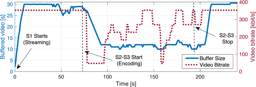
Figure 1. Effect of coupling on joint networking-MEC slicing.

We further verify this critical issue in Fig. 1, where we show an experiment (testbed described in Section 8) where we instantiate 1 slice for video streaming (S1) and 2 slices for video transcoding (S2 and S3). S1 starts at $t=0$, while S2 and S3 start at $t=75$. Fig. 1 clearly shows that as soon as S2 and S3 start, the performance of S1 plummets. This is because the computational resources allocated for S2 and S3 cause the video buffer (blue line) to drop from $\sim$30 seconds to $\sim$10 seconds, which in turn causes highly-jittered bitrate (red line). As soon as S2 and S3 end at $t=190$, buffer size and video bitrate sharply increase and stabilize. This demonstrates that slices that require both computation and networking resources (S1, video streaming) are inevitably impacted by slices running on the same node that only require computation (S2 and S3, video transcoding). Therefore, taking into account the coupling among slices is a compelling necessity to guarantee appropriate performances when designing edge slicing algorithms.

Extensive research efforts have already explored MEC algorithms for cellular networks and network slicing (Liu and Han, 2019; Van Huynh et al., 2019; Castellano et al., 2019; Ndikumana et al., 2019). The key limitation of prior work, however, is the assumption that network slicing and MEC are distinct problems. As we demonstrated in Fig. 1, this is hardly the case in practical scenarios. However, the already rich literature on network slicing—discussed in detail in Section 2—has not yet considered this fundamental aspect. This makes the joint MEC/slicing paradigm a substantially unexplored problem. We also point out that due to the massive scale envisioned for 5G and IoT applications, centralized algorithms become prohibitive. Thus, a core issue is not only to account for resource coupling, but also to devise new slicing algorithms that provide highly efficient and scalable slicing strategies.

Novel contributions. The paper’s key innovation is the design, analysis and experimental evaluation of the unified MEC slicing framework, called Sl-EDGE, that allows network operators to instantiate heterogeneous slice services (e.g., video streaming, caching, 5G network access) on edge devices. In a nutshell, we make the following novel contributions;

$\bullet$ We mathematically model and discuss coupling relationships among networking, storage and computation resources at each edge node (Section 4). We formulate the Edge Slicing Problem (ESP) as a Mixed Integer Linear Programming (MILP) problem, and we prove that it is NP-hard (Section 5);

$\bullet$ We propose three novel slicing algorithms to address (ESP), each having different optimality and computational complexity. Specifically, we present (i) a centralized optimal algorithm for small network instances (Section 5); (ii) an approximation algorithm that leverages virtualization concepts to reduce complexity with close-to-optimal performance (Section 6.1), and (iii) a low-complexity algorithm where slicing decisions are made at the edge nodes with minimal overhead (Section 6.2);

$\bullet$ We extensively evaluate the performance of the three slicing algorithms through simulation, and compare Sl-EDGE with DIRECT (Liu and Han, 2019), to the best of our knowledge the state-of-the-art slicing framework for MEC 5G applications (Section 7). Our results show that, by taking into account coupling among heterogeneous resources, Sl-EDGE (i) instantiates slices 6x more efficiently then the algorithm proposed in (Liu and Han, 2019), as well as satisfying resource availability constraints; (ii) can be implemented with a distributed approach while getting 0.25 close to the optimal solution;

$\bullet$ We prototype and demonstrate Sl-EDGE on a testbed composed by 24 software-defined radios. Experimental results demonstrate that Sl-EDGE instantiates heterogeneous slices providing LTE connectivity to smartphones, video streaming over WiFi, and ffmpeg video transcoding while achieving an instantaneous throughput of $37\>\mathrm{Mbit/s}$ over LTE links, $1.2\>\mathrm{Mbit/s}$ video streaming bitrate with an overall CPU utilization of $83\%$ (Section 8).

2. Related Work

Motivated by the ever increasing interests from both NOs and standardization entities (ETSI, 2019b, a, 2018b), network slicing and multi-access edge computing technologies have recently become “all the rage” in the wireless research community (Mancuso et al., 2019; D’Oro et al., 2019; Mandelli et al., 2019; Garcia-Aviles et al., 2018; Rost et al., 2017; Zhang et al., 2019; Foukas et al., 2017). Lately, we have seen a deluge of algorithms to efficiently slice portions of the network and instantiate service-specific slices. These solutions leverage optimization (Han et al., 2019; Halabian, 2019; Sun et al., 2019; Agarwal et al., 2018), game-theory (Caballero et al., 2017; Jiang et al., 2017; D’Oro et al., 2018) and machine learning (Van Huynh et al., 2019) tools.

Concurrently, MEC has demonstrated to be an effective methodology to significantly reduce latency. This paradigm has been successfully used to provide task offloading (Misra and Saha, 2019; Tran and Pompili, 2018; Liu et al., 2016; Wang et al., 2019), augmented reality (AR) (Al-Shuwaili and Simeone, 2017; Erol-Kantarci and Sukhmani, 2018; Tang and He, 2018), low-latency video streaming (He et al., 2019; Yang et al., 2018), and caching (Hoang et al., 2018; Zhang et al., 2018), among others. We refer the interested reader to the following surveys for a more detailed overview of network slicing and MEC (Afolabi et al., 2018; Kaloxylos, 2018; Taleb et al., 2017; Mao et al., 2017; Mach and Becvar, 2017).

These works are extremely effective when the two technologies are considered as independent entities operating on the same infrastructure. However, as shown in Fig. 1, they are prone to resource over-provisioning when both technologies coexist on the same edge nodes and share the same resources. Ndikumana et al. (Ndikumana et al., 2019) consider the allocation of heterogeneous resources for task offloading problems in MEC ecosystems, while in (Agarwal et al., 2018) Agarwal et al. consider the problem of jointly allocating CPUs and virtual network functions for network slicing applications. Similarly, in (Van Huynh et al., 2019) Van Huynh et al. account for slice networking, computation, and storage resources by designing a deep dueling neural network that determines which slices to be admitted, maximizes the network provider’s reward, and avoids resource over-provisioning. Although (Van Huynh et al., 2019) accounts for resource heterogeneity, the authors only focus on the slicing admission control problem, and do not consider how to partition the resources of each slice among the nodes of the network. A heterogeneous resource orchestration framework for edge computing ecosystems called Senate is presented by Castellano et al. in (Castellano et al., 2019). Senate leverages Distributed Orchestration Resource Assignment (DORA) and election algorithms to allow the instantiation of multiple virtual network functions on the same infrastructure. However, this work focuses on the wired portion of the edge network only.

The closest work to ours is (Liu and Han, 2019), where Liu and Han proposed a distributed slicing framework for MEC-enabled wireless networks called DIRECT. Despite being extremely successful in slicing networks with MEC resources residing in dedicated servers close to the base stations, DIRECT does not account for the case where both networking and MEC resources coexist on the same edge node.

This paper separates itself from prior work as it makes a substantial step forward toward the coexistence of network slicing and MEC technologies. Indeed, we consider the challenging case of edge nodes jointly providing wireless network access and MEC functionalities to mobile users. Furthermore, we model the intrinsic coupling among heterogeneous resources residing on edge nodes, and design Sl-EDGE, a slicing framework that leverages such a coupling to instantiate heterogeneous slices on the same physical infrastructure.

3. Sl-EDGE at a glance

Sl-EDGE is a slicing framework for MEC-enabled 5G systems. Its key advantage is that it provides a fast, flexible and efficient deployment of joint networking and MEC slices. The three-tiered architecture of Sl-EDGE is illustrated in Fig. 2.

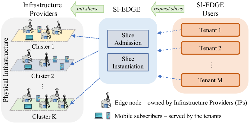
Figure 2. The three-tier architecture of Sl-EDGE.

The physical infrastructure consists of a set of MEC-enabled networking edge nodes (e.g., base stations, access points, IoT gateways)—referred to as MEC hosts (ETSI, 2018b)—controlled by one or more Infrastructure Providers (IPs). MEC hosts are located at the network edge and simultaneously provide networking, storage and computational services (e.g., Internet access, video content delivery, caching).

Sl-EDGE Users are both mobile and virtual NOs and Service Providers (SPs)—referred to as the tenants—willing to rent portions of the infrastructure to provide services to their subscribers. Tenants access Sl-EDGE to visualize relevant information such as position of MEC hosts, which areas they cover and a list of networking and MEC services that can be instantiated on each host (e.g., 5G/WiFi connectivity, caching, computation). Whenever tenants need to provide these services, they submit slice requests to obtain networking, storage or computation resources. The received slice requests are collected and processed by Sl-EDGE which (i) determines the set of requests to be accommodated by using centralized (Section 5) and distributed algorithms (Section 6); (ii) instantiates slices by allocating the available resources to each admitted slice, and (iii) notifies to the admitted tenants the list of the resources allocated to the slice.

4. System model

Let $\mathcal{D}$ be the set of deployed MEC-enabled networking devices, or edge nodes. Edge nodes provide both wireless connectivity and MEC services to a limited portion of the network. Therefore, they can be clustered into $K$ clusters located in different geographical areas (Ndikumana et al., 2019; Bouet and Conan, 2018; Gudipati et al., 2013). Let $\mathcal{K}=\{1,2,\dots,K\}$ be the set of these $K$ independent clusters, and let $\mathcal{D}_{k}$ be the set of edge nodes in cluster $k\in\mathcal{K}$. Each edge node $d\in\mathcal{D}_{k}$ is equipped with a set of networking, storage and computational capabilities, usually measured in terms of number of RBs (D’Oro et al., 2019), megabytes, and billion of instructions per second (GIPS) (Ndikumana et al., 2019), respectively. Let $z\in\mathcal{T}=\{\mathcal{N},\mathcal{S},\mathcal{C}\}$ represent the resource type, i.e., networking ($\mathcal{N}$), storage ($\mathcal{S}$), and computing ($\mathcal{C}$). Moreover, let $\boldsymbol{\rho}_{d}=(\rho_{d}^{z})_{z\in\mathcal{T}}\in\mathbb{R}_{\geq 0}^{3}$ be the set of resources available at each edge node $d$. An example of the physical infrastructure and its clustered structure is shown in Fig. 3.

Let $\mathcal{R}=\{\mathcal{R}^{\mathcal{N}},\mathcal{R}^{\mathcal{S}},\mathcal{R}^{\mathcal{C}}\}$ be the set of slice requests submitted to Sl-EDGE, with $\mathcal{R}^{\mathcal{N}},\mathcal{R}^{\mathcal{S}},\mathcal{R}^{\mathcal{C}}$ being the set for networking, storage, and computing slice requests, respectively. Each request $r\in\mathcal{R}^{z}$ of type $z$ is associated to a value $v_{r}^{z}>0$ used by the IP to assess the importance—or monetary value—of $r$. Also, we define the $K$-dimensional request demand array $\boldsymbol{\tau}_{r}=(\tau^{z}_{r,k})_{k\in\mathcal{K}}$, where $\tau^{z}_{r,k}\geq 0$ represents the amount of resources of type $z$ requested by $r$ in cluster $k$. Without loss of generality, we assume that $\sum_{k\in\mathcal{K}}\tau^{z}_{r,k}>0$ for all $r\in\mathcal{R}$.

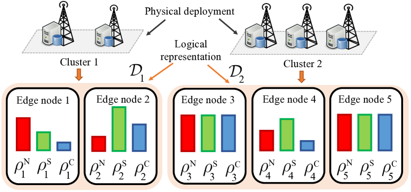
Figure 3. System model example with $K=2$ clusters with edge node sets $\mathcal{D}_{1}=\{1,2\}$ and $\mathcal{D}_{2}=\{3,4,5\}$, respectively.

4.1. Resource coupling and collateral functions

To successfully slice networking and MEC resources, it is paramount to understand the underlying dynamics between resources of different nature. To this purpose, let us consider two simple but extremely effective examples.

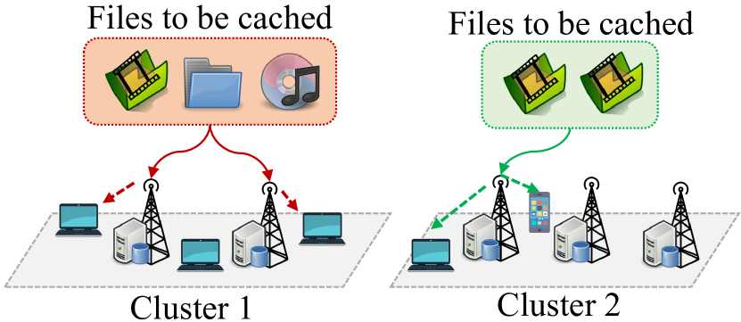
Figure 4. Content caching.

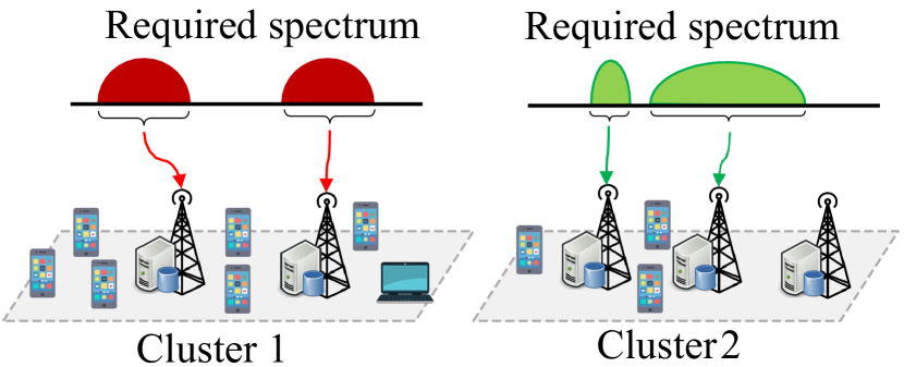
Figure 5. 5G networking.

4.1.1. Content Caching

a tenant instantiates a storage slice (Fig. 5) to provide caching services to its subscribers, i.e., $r\in\mathcal{R}^{\mathcal{S}}$, and specifies how many megabytes ($\tau_{r,k}^{\mathcal{S}}$) should be allocated in each cluster $k\in\mathcal{K}$. In this case, the content to be cached should be (i) first transmitted and then (ii) processed by storing edge nodes. Therefore, storage activities related to caching procedures not only utilize storage resources, but also require networking and computational resources.

4.1.2. 5G networking

in this example (Fig. 5) a tenant wants to provide cellular services to mobile subscribers. Hence, it submits a networking slice request $r$ of type $\mathcal{N}$ and specifies the clusters to be included in the slice and the amount of spectrum resources ($\tau_{r,k}^{\mathcal{N}}$) needed in each cluster. Edge nodes providing connectivity must (i) perform channel estimation and baseband signal processing procedures, and (ii) locally cache or buffer the data to transmit. Therefore, the allocation of resources of type $\mathcal{N}$ entails resources of type $\mathcal{C}$ and $\mathcal{S}$.

These two examples suggest that heterogeneous resources are tightly intertwined, thus motivating the need for new slicing algorithms that account for these intrinsic relationships. To incorporate coupling within the Sl-EDGE framework, we introduce the concept of collateral functions.

Let us consider the case where, to instantiate a slice of type $z\in\mathcal{T}$, $x$ resources must be allocated on edge node $d\in\mathcal{D}_{k},k\in\mathcal{K}$. For any resource type $t\in\mathcal{T}\setminus\{z\}$, we define the collateral function $\alpha_{d,k}^{z\rightarrow t}(x):\mathbb{R}\rightarrow\mathbb{R}$. This function (i) reflects coupling among heterogeneous resources, and (ii) determines how many resources of type $t$ should be allocated on edge node $d$ when allocating $x$ resources of type $z$. Of course, $\alpha_{d,k}^{z\rightarrow z}(x)=x$.

In this paper, we model resource coupling as an increasing linear function with respect to $x$. This way, the number of resources of type $z$ needed to instantiate $x$ resources of type $t$ on a given edge node $d$ can be evaluated as $\alpha_{d,k}^{t\rightarrow z}(x)=A_{d,k}^{t\rightarrow z}x$, with $A_{d,k}^{t\rightarrow z}$ being measured in units of type $z$ per unit of type $t$, e.g., GIPS per megabyte. However, the more general case where $\alpha_{d,k}^{t\rightarrow z}(x)$ is a non-linear function can be easily related to the linear case by using well-established and accurate piece-wise linearization techniques (Lin et al., 2013). For any $k\in\mathcal{K}$ and $d\in\mathcal{D}_{k}$, let $\mathbf{A}_{d,k}$ be the collateral matrix for edge node $d$. Such a matrix can be written as

(1) $$\mathbf{A}_{d,k}=\left(\begin{matrix}1&A_{d,k}^{\mathcal{S}\rightarrow\mathcal{N}}&A_{d,k}^{\mathcal{C}\rightarrow\mathcal{N}}\\ A_{d,k}^{\mathcal{N}\rightarrow\mathcal{S}}&1&A_{d,k}^{\mathcal{C}\rightarrow\mathcal{S}}\\ A_{d,k}^{\mathcal{N}\rightarrow\mathcal{C}}&A_{d,k}^{\mathcal{S}\rightarrow\mathcal{C}}&1\end{matrix}\right).$$

5. Edge slicing problem and its optimal solution

The key targets of Sl-EDGE are to (i) maximize profits generated by infrastructure slice rentals, and (ii) allow location-aware and dynamic instantiation of slices in multiple clusters, while (iii) avoiding over-provisioning of resources to avoid congestion and poor performance. We formalize the above three targets with the edge slicing optimization problem (ESP) introduced below.

(ESP) $$\underset{\mathbf{y},\boldsymbol{\sigma}}{\text{maximize}} \sum_{k\in\mathcal{K}}\sum_{z\in\mathcal{T}}\sum_{r\in\mathcal{R}^{z}}v^{z}_{r}y^{z}_{r}$$

(2) subject to $$\sum_{d\in\mathcal{D}_{k}}\sigma_{r,d}^{z}=\tau_{r,k}^{z}y_{r}^{z},\hskip 1.42271pt\forall z\in\mathcal{T},k\in\mathcal{K},r\in\mathcal{R}^{z}$$

(3) $$\sum_{r\in\mathcal{R}^{z}}\!\sum_{t\in\mathcal{T}}\!\!\alpha_{d,k}^{t\rightarrow z}(\sigma_{r,d}^{t})\!\leq\!\rho_{d,k}^{z},\hskip 1.42271pt\forall\!z\!\in\!\mathcal{T},k\!\in\!\mathcal{K},d\!\in\!\mathcal{D}_{k}$$

(4) $$y_{r}^{z}\in\{0,1\},\hskip 5.69046pt\forall z\in\mathcal{T},r\in\mathcal{R}^{z}$$

(5) $$\sigma_{r,d}^{z}\geq 0,\hskip 2.84544pt\forall z\in\mathcal{T},r\in\mathcal{R}^{z},k\in\mathcal{K},d\in\mathcal{D}_{k}$$

where $\mathbf{y}=(y_{r}^{z})_{z\in\mathcal{T},r\in\mathcal{R}^{z}}$ and $\boldsymbol{\sigma}=(\sigma_{r,d}^{z})_{z\in\mathcal{T},r\in\mathcal{R}^{z},d\in\mathcal{D}}$ respectively are the slice admission and resource slicing policies. Quantity $y_{r}^{z}$ is a binary variable such that $y_{r}^{z}=1$ if request $r$ is admitted, $y_{r}^{z}=0$ otherwise. Similarly, $\sigma_{r,d}^{z}$ represents the amount of resources of type $z$ that are assigned to $r$ on edge node $d$.

One can easily verify that Problem (ESP) meets the previously mentioned requirements, since it (i) aims at maximizing the total value of the admitted slice requests; (ii) guarantees that each admitted slice obtains the required amount of resources in each cluster (Constraint (2)), and (iii) prevents resource over-provisioning on each edge node (Constraint (3)).

Given the presence of both continuous and 0-1 variables, (ESP) belongs to the class of MILPs problems, well-known to be hard to solve. More precisely, in Theorem 1 we will prove that (ESP) is NP-hard even in the case of requests having the same value and edge nodes belonging to a single cluster.

Theorem 1 (NP-hardness).

Problem (ESP) is NP-hard.

Proof.

To prove this theorem, we reduce the Splittable Multiple Knapsack Problem (SMKP), which is NP-hard (Miyazaki et al., 2015), to an instance of (ESP). Let us assume that all edge nodes belong to the same cluster $k$ and all submitted slice requests are of the same type $z\in\mathcal{T}$. Furthermore, we assume that all requests have value $v_{r}^{z}=v_{s}^{z}=1$ for any $(r,s)\in\mathcal{R}\times\mathcal{R}$. Since all requests are of the same type $z$, $\alpha_{d,k}^{z\rightarrow z}(x)=x$ for any edge node $d\in\mathcal{D}$. Let us now consider the SMKP, whose statement is as follows: given a set of knapsacks (the edge nodes) with limited capacity ($\rho^{z}_{d,k}$) and a set of items (requests) with certain value ($v_{r}^{z}$) and size ($\tau^{z}_{r,k}$), assume that items can be split among the knapsacks while satisfying Constraint (2), is there an allocation policy that maximizes the total number of items added to the knapsacks without overfilling them? We observe that Problem (ESP) is a reduction of the SMKP. Since this reduction can be built in polynomial time, it follows that Problem (ESP) is NP-hard. ∎

Problem (ESP) can be solved by means of efficient and well-established exact Branch-and-Cut (B&C) algorithms. Even though the worst-case complexity of such algorithms is exponential, B&C leverages structural properties of the problem to confine the search space, thus reducing the time needed to compute an optimal solution. The B&C procedure—not reported here for the sake of space—can be found in (Elf et al., 2001). We now focus on how to overcome some of the limitations of B&C. Specifically, B&C suffers from high computational complexity, and requires a centralized entity with perfect knowledge, both of which are unacceptable in large-scale and dynamic networks.

6. Approximation Algorithms

We now design two approximation algorithms for (ESP) whose primary objective is to (i) reduce the computational complexity of the problem, and (ii) minimize the overhead traffic traversing the network. In Section 6.1 and Section 6.2, we present the algorithmic implementation of the two algorithms, and further discuss their optimality, complexity and overhead.

6.1. Decentralization through virtualization

One of the main sources of complexity in Problem (ESP) is the large number of optimization variables $\bf{y}$ and $\boldsymbol{\sigma}$. However, we notice that $R=\sum_{z\in\mathcal{T}}|\mathcal{R}^{z}|$, where $|\cdot|$ is the set cardinality operator. On the contrary, the number of $\boldsymbol{\sigma}$ variables is $\mathcal{O}(RD)$, with $D$ being the total number of edge nodes in the infrastructure. While $R$ is generally limited to a few tens of requests, the number $D$ of edge nodes deployed in the network might be very large. However, a big portion of these edge nodes are equipped with hardware and software components that are either similar or exactly the same. Thus, we can leverage similarities among edge nodes to reduce the complexity of Problem (ESP) while achieving close-to-optimal solutions and reduced control overhead.

Edge nodes with similar collateral functions will behave similarly. However, being similar in terms of $\alpha$ only does not suffice to determine whether or not two edge nodes are similar. In fact, nodes with similar $\alpha$ might have a different amount of available resources. For this reason, we leverage the concept of similarity functions (Huang, 2008).

Definition 0.

Let $\Delta(d^{\prime},d^{\prime\prime}):\mathcal{D}\times\mathcal{D}\rightarrow\mathbb{R}$ be a function to score the similarity between edge nodes $d^{\prime}$ and $d^{\prime\prime}$. Two edge nodes $d^{\prime},d^{\prime\prime}\in\mathcal{D}$ are said to be $\epsilon$-similar with respect to $f$ if $\Delta(d^{\prime},d^{\prime\prime})\leq\epsilon$, for any $\epsilon\in\mathbb{R}_{\geq 0}$. If $\Delta(d^{\prime},d^{\prime\prime})=0$, we say that $d^{\prime}$ and $d^{\prime\prime}$ are identical.

Through $\epsilon$-similarity, we can first determine which edge nodes inside the same cluster are similar, and then abstract their physical properties to generate a virtual edge node. For the sake of generality, in this paper we do not make any assumption on $\Delta(\cdot)$ (interested readers are referred to (Xu and Wunsch, 2005) for an exhaustive survey on the topic). However, the impact of $\Delta(\cdot)$ and $\epsilon$ on the overall system performance will be first discussed in Section 6.1.1, and then evaluated in Section 7.

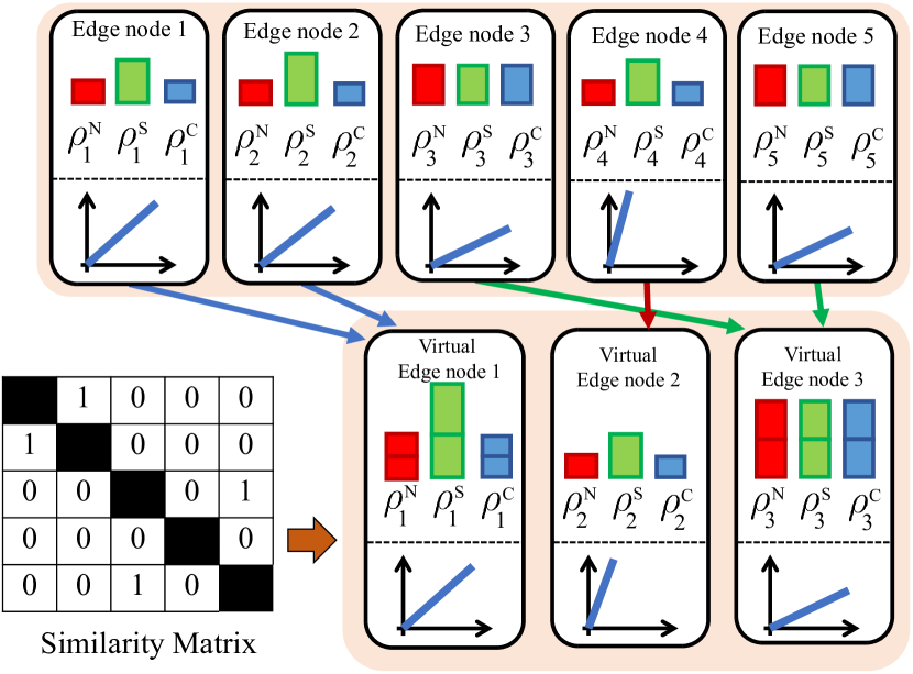
Figure 6. An example of the virtual edge node generation in Step 1. The similarity matrix determines which edge nodes can be aggregated. Similar edge nodes (i.e., $\{1,2\}$ and $\{3,5\}$) are aggregated into virtual ones. Edge node 4 is not aggregated as it has similar resources to $\{1,2\}$, but different collateral function.

Now we present V-ESP, an approximation algorithm that leverages virtualization concepts to compute a solution to Problem (ESP). The main steps of V-ESP are as follows:

$\bullet$ Step 1: (Virtual edge node generation): for each cluster $k$, we build the $|\mathcal{D}_{k}|\times|\mathcal{D}_{k}|$ similarity matrix $\mathcal{S}_{k}$. For any real $\epsilon\geq 0$, element $s_{d^{\prime},d^{\prime\prime}}\in\mathcal{S}_{k}$ indicates whether or not $d^{\prime}$ and $d^{\prime\prime}$ are $\epsilon$-similar. That is, $s_{d^{\prime},d^{\prime\prime}}=1$ if $\Delta(d^{\prime},d^{\prime\prime})\leq\epsilon$, $s_{d^{\prime},d^{\prime\prime}}=0$ otherwise. We partition the set $\mathcal{D}_{k}$ into $G_{k}\geq 1$ independent subsets that contain similar edge nodes only. Partitions are generated such that $\bigcup_{g=1}^{G_{k}}\mathcal{D}_{k,g}=\mathcal{D}_{k}$ and $\mathcal{D}_{k,j}\cap\mathcal{D}_{k,i}=\emptyset$ for any $i,j=1,2,\dots,G_{k}$.

Each non-singleton partition is converted into a virtual edge node. Specifically, for each non-singleton partition $\mathcal{D}_{k,g}$, we define a virtual edge node $\tilde{d}_{g}$ whose available resources are equal to the sum of the available resources of all edge nodes in the partition, i.e., $\rho^{z}_{\tilde{d}_{g},k}=\sum_{d\in\mathcal{D}_{k,g}}\rho^{z}_{d,k}$. The collateral function of the virtual edge node $d_{g}^{v}$ is constructed as $\alpha_{\tilde{d}_{g},k}^{t\rightarrow z}=f(\mathcal{D}_{k,g},t,z)$, where $f(\cdot)$ is a function that generates a virtualized collateral function for virtual edge node $\tilde{d}_{g}$ discussed in Section 6.1.1. We show an example of virtualization procedure in Fig. 6.

$\bullet$ Step 2: (Virtual Edge Nodes Advertisement): each cluster $k$ advertises Sl-EDGE the set $\mathcal{D}_{k}=(\tilde{d}_{g})_{g=1,\dots,G_{k}}$ of $G_{k}$ virtualized edge nodes, as well as their virtual collateral functions ($\alpha_{\tilde{d}_{g},k}^{t\rightarrow z}$) and available resources ($\rho^{z}_{\tilde{d}_{g},k}$).

$\bullet$ Step 3: (Solve virtualized ESP): Sl-EDGE solves Problem (ESP) with virtualized edge nodes through B&C. Slice admission and resource slicing policies $(\bf{\tilde{y}}^{*},\boldsymbol{\tilde{\sigma}}^{*})$ are computed and each cluster receives the $2$-tuple $(\bf{\tilde{y}}^{*},\boldsymbol{\tilde{\sigma}}^{*}_{k})$, with $\boldsymbol{\tilde{\sigma}}^{*}_{k}=(\tilde{\sigma}^{z*}_{r,\tilde{d}_{g}})_{z\in\mathcal{T},r\in\mathcal{R},g=1,\dots,G_{k}}$ being the resource allocation policy over the virtualized edge nodes of cluster $k$.

$\bullet$ Step 4: (Virtualized edge node resource allocation): upon receiving $(\bf{\tilde{y}}^{*},\boldsymbol{\tilde{\sigma}}^{*}_{k})$, cluster $k$ solves $G_{k}$ Linear Programming (LP) problems in parallel, one for each virtual edge node $g$. These LPs are formulated as follows:

(6) find $$\hskip 8.5359pt\boldsymbol{\sigma}_{k,g}$$

(7) subject to $$\hskip 8.5359pt\sum_{d\in\mathcal{D}_{k,g}}\sigma_{r,d}^{z}=\tilde{\sigma}^{z*}_{r,\tilde{d}_{g}},\hskip 2.84544pt\forall r\in\mathcal{R}$$

$$\hskip 2.84544pt\mbox{Constraints}~{}\eqref{eq:c2},~{}\eqref{eq:c4}$$

which can be optimally solved by computing any feasible resource allocation policy that satisfies all constraints.

$\bullet$ Step 5: (Slicing Policies Construction): let $\boldsymbol{\sigma}^{*}_{k,g}=(\boldsymbol{\sigma}^{*}_{k,d})_{d\in\mathcal{D}_{k,g}}$ be the optimal solution of the $g$-th instance of (6). The resource slicing policy $\boldsymbol{\sigma}^{*}_{k}$ for cluster $k$ is constructed by stacking all $G_{k}$ individual solutions computed by individual clusters, i.e., $\boldsymbol{\sigma}^{*}_{k}=(\boldsymbol{\sigma}^{*}_{k,g})_{g=1,\dots,G_{k}}$. The final slice admission and resource slicing policies are $(\bf{\tilde{y}}^{*},\boldsymbol{\sigma}^{*})$ with $\boldsymbol{\sigma}^{*}=(\boldsymbol{\sigma}^{*}_{k})_{k\in\mathcal{K}}$.

Through V-ESP, each cluster exposes $G_{k}\leq|\mathcal{D}_{k}|$ virtual edge nodes only, rather than $|\mathcal{D}_{k}|$ (Steps 1-2). Thus, virtualization reduces the number of edge nodes and thus the number of variables in (ESP). Moreover, since virtualization leaves the structure of the slicing problem unchanged, we efficiently solve Step 3 through the same B&C techniques used for (ESP). In addition, while Steps 3-5 are executed whenever a new slicing policy is required (e.g., tenants submit new slice requests or the slice rental period expires), Steps 1-2 are executed only when the structure of the physical infrastructure changes (e.g., edge nodes are turned on/off or are subject to hardware modifications). This way, we can further reduce the overhead. In short, V-ESP splits the computational burden among the NO (Step 3) and the edge nodes (Steps 1-2 and 4), which jointly provides the high efficiency typical of centralized approaches while enjoying reduced complexity of decentralized algorithms.

6.1.1. Design Aspects of Virtualization

Step 1 relies on $\epsilon$-similarity to aggregate edge nodes and reduce the search space. Intuitively, the higher the value of $\epsilon$, the smaller the set of virtual edge nodes generated in Step 1, the faster Sl-EDGE computes solutions in Step 3. However, large $\epsilon$ values might group together edge nodes with different available resources and collateral functions. In this case, (i) Step 1 might produce virtual edge nodes that poorly reflect physical edge nodes features, and (ii) solutions computed at Step 3 might not be feasible when applied to Step 4. Thus, there is a trade-off between accuracy and computational speed, which will be the focus of Section 7.4.

Another aspect that influences the efficiency and feasibility of solutions generated by the V-ESP algorithm is the function $f(\cdot)$, which transforms collateral functions of similar edge nodes into an aggregated collateral function. Recall that $f(\cdot)$, which can be represented as a collateral matrix (1), must mimic the actual behavior of physical edge nodes belonging to the same partition $g$. To avoid overestimating the capabilities of virtual edge nodes, and producing unfeasible solutions, the generic element of the virtual collateral matrix (1) for virtual edge node $\tilde{d}_{g}$ is set to $A_{\tilde{d}_{g},k}^{z\rightarrow t}=\max_{d\in\mathcal{D}_{k,g}}\{A_{d,k}^{z\rightarrow t}\},\forall z,t\in\mathcal{T}$. Although this model underestimates the capabilities of physical edge nodes and may admit less requests than the optimal algorithm, it always produces feasible solutions in Steps 3 and 4.

6.2. Distributed Edge Slicing

In this section we design a distributed edge slicing algorithm for Problem (ESP) such that clusters can locally compute slicing strategies. We point out that making (ESP) distributed is significantly challenging. In fact, both utility function and constraints are coupled with each other through the optimization variables $\boldsymbol{\sigma}$ and $\mathbf{y}$. This complicates the decomposition of the problem into multiple independent sub-problems.

In order to decouple the problem into multiple independent sub-problems, we introduce the auxiliary variables $\mathbf{y}_{k}=(y^{z}_{r,k})_{z\in\mathcal{T},r\in\mathcal{R}^{z}}$ such that $y^{z}_{r,k}=y^{z}_{r}$ for any request $r$ and cluster $k$. Thus, Problem (ESP) can be rewritten as

(D-ESP) $$\underset{\boldsymbol{\sigma},\mathbf{y}}{\text{maximize}} \hskip 5.69046pt\frac{1}{|\mathcal{K}|}\sum_{k\in\mathcal{K}}\sum_{z\in\mathcal{T}}\sum_{r\in\mathcal{R}^{z}}v_{r}^{z}y^{z}_{r,k}$$

(8) subject to $$\hskip 2.84544pt\sum_{d\in\mathcal{D}_{k}}\sigma_{r,d}^{z}=\tau_{r,k}^{z}y_{r,k}^{z},\hskip 2.84544pt\forall z\in\mathcal{T},k\in\mathcal{K},r\in\mathcal{R}^{z}$$

(9) $$\hskip 5.69046pty_{r,k}^{z}=y_{r,m}^{z},\hskip 5.69046pt\forall z\in\mathcal{T},(k,m)\in\mathcal{K}^{2},r\in\mathcal{R}^{z}$$

(10) $$\hskip 5.69046pty_{r,k}^{z}\in\{0,1\}\hskip 5.69046pt\forall z\in\mathcal{T},r\in\mathcal{R}^{z}$$

$$\hskip 5.69046pt\mbox{Constraints}~{}\eqref{eq:c2},~{}\eqref{eq:c4}\vspace{-0.7cm}$$

where $\mathbf{y}=(y_{r,k}^{z})_{z\in\mathcal{T},r\in\mathcal{R}^{z},z\in\mathcal{T}}$, while Constraint (9) guarantees that different clusters admit the same requests.

Problem (D-ESP) is with separable variables with respect to the $K$ clusters. That is, Problem (D-ESP) can be split into $K$ sub-problems, each of them involving only variables controlled by a single cluster. To effectively decompose Problem (D-ESP) we leverage the Alternating Direction Method of Multipliers (ADMM) (Boyd et al., 2011). The ADMM is a well-established optimization tool that enforces constraints through quadratic penalty terms and generates multiple sub-problems that can be iteratively solved in a distributed fashion.

The augmented Lagrangian for Problem (D-ESP) can be written as follows:

$$L(\boldsymbol{\sigma},\mathbf{y},\boldsymbol{\lambda},\rho) =\sum_{k\in\mathcal{K}}\sum_{z\in\mathcal{T}}\sum_{r\in\mathcal{R}^{z}}v_{r}^{z}y^{z}_{r,k}$$

$$-\sum_{z\in\mathcal{T}}\sum_{r\in\mathcal{R}^{z}}\sum_{k\in\mathcal{K}}\sum_{m\in\mathcal{K}}\lambda^{z}_{r,k,m}(y^{z}_{r,k}-y^{z}_{r,m})$$

(11) $$-\frac{\rho}{2}\sum_{z\in\mathcal{T}}\sum_{r\in\mathcal{R}^{z}}\sum_{k\in\mathcal{K}}\sum_{m\in\mathcal{K}}(y^{z}_{r,k}-y^{z}_{r,m})^{2}$$

where $\boldsymbol{\lambda}=(\lambda^{z}_{r,k,m})$ are the so-called dual variables, and $\rho>0$ is a step-size parameter used to regulate the convergence speed of the distributed algorithm (Boyd et al., 2011).

Let $k\in\mathcal{K}$, we define $\mathbf{y}_{-k}=(\mathbf{y}_{m})_{m\in\mathcal{K}\setminus\{k\}}$ which identifies the slice admission policies taken by all clusters except for cluster $k$. Similarly, we define $\boldsymbol{\sigma}_{-k}=(\boldsymbol{\sigma}_{m})_{m\in\mathcal{K}\setminus\{k\}}$. Problem (D-ESP) can be solved through the following ADMM-based iterative algorithm

(12) $$\{\mathbf{y}_{k},\boldsymbol{\sigma}_{k}\}(t\!+\!1) =\operatorname*{argmax}_{\mathbf{y}_{k},\boldsymbol{\sigma}_{k}}L(\boldsymbol{\sigma}_{k},\mathbf{y}_{k},\boldsymbol{\sigma}_{-k}(t),\mathbf{y}_{-k}(t),\boldsymbol{\lambda}(t),\rho)$$

(13) $$\lambda^{z}_{r,k,m}(t\!+\!1) =\lambda^{z}_{r,k,m}(t)+\rho(y^{z}_{r,k}(t+1)-y^{z}_{r,m}(t+1))$$

where each cluster sequentially updates $\mathbf{y}_{k}$ and $\boldsymbol{\sigma}_{k}$, while the dual variables $\boldsymbol{\lambda}$ are updated as soon as all clusters have updated their strategy according to (12). To update (12) each cluster solves the following quadratic problem

(DC-ESP) $$\underset{\boldsymbol{\sigma}_{k},\mathbf{y}_{k}}{\text{maximize}} \!\sum_{z\in\mathcal{T}}\!\sum_{r\in\mathcal{R}^{z}}\!\tilde{v}^{z}_{r,k}(\mathbf{y}_{-k}(t\!-\!1),\boldsymbol{\lambda}(t\!-\!1))y^{z}_{r,k}\!-\!2\rho(y^{z}_{r,k})^{2}$$

subject to $$\hskip 5.69046pt\mbox{Constraints}~{}\eqref{eq:c2},~{}\eqref{eq:c4},~{}\eqref{eq:desp:c1},~{}\eqref{eq:desp:c2},$$

where $\tilde{v}^{z}_{r,k}$ is the adjusted value of request $r$ defined as

$$\tilde{v}^{z}_{r,k}(\mathbf{y}_{-k}(t),\boldsymbol{\lambda}(t)) =v^{z}_{r,k}-\sum_{m\in\mathcal{K}\setminus\{{k}\}}\left(\lambda^{z}_{r,k,m}(t)-\lambda^{z}_{r,m,k}(t)\right)$$

(14) $$+\rho~{}\phi_{r,k}(\mathbf{y}_{-k}(t))$$

and $\phi_{r,k}(\mathbf{y}_{-k}(t))=\sum_{m\in\mathcal{K}\setminus\{{k}\}}y^{z}_{r,m}(t)$ is used by cluster $k$ to obtain the number of clusters that have accepted request $r$.

The advantages of Problem (DC-ESP) are that (i) clusters do not need to advertise the composition of the physical infrastructure to the IP or to other clusters, and (ii) it can be implemented in a distributed fashion. Indeed, at any iteration $t$, the only parameters needed by cluster $k$ to solve (12) are the dual variables $\boldsymbol{\lambda}(t-1)$ and the number $\phi_{r,k}(\mathbf{y}_{-k}(t))$ of clusters that admitted the request $r$ at the previous iteration.

It has been shown that ADMM usually enjoys linear convergence (Shi et al., 2014), but improper choices of $\rho$ might generate oscillations. To overcome this issue and achieve convergence, we implemented the approach proposed in (Boyd et al., 2011, Eq. (3.13)) where $\rho$ is updated at each iteration of the ADDM. The optimality and convergence properties of DC-ESP will be exstensively evaluated in Figs. 10 and 11.

7. Numerical Results

We now assess the performance of the three slicing algorithms described in Section 5 and Section 6 by (i) simulating a MEC-enabled 5G network, and by (ii) comparing the algorithms with the recently-published DIRECT framework (Liu and Han, 2019).

We consider a scenario where edge nodes provide mobile subscribers with 5G NR connectivity as well as storage and computation MEC services, such as caching and video decoding. We assume that (i) edge nodes share the same NR numerology—more precisely, networking resources are arranged over an OFDM-based resource grid with 50 RBs, and (ii) edge nodes are equipped with hardware components with up to 1 Terabyte of storage capabilities and a maximum of 200 GIPS. We fix the number of RBs for each edge node, while we randomly generate the amount of computation and storage resources at each simulation run. To simulate a realistic scenario with video transmission, storage and transcoding applications, collateral matrices in (1) are generated by randomly perturbing the following matrix $\mathbf{A}^{0}=[1,0.0382,0.1636;26.178,1,0.0063;0.49,0.15,1]$ at each run. To give an example, processing a data rate of $15.264$ Mbit/s (equivalent to LTE 16-QAM with 50 RBs) requires $24.4224$ GIPS (e.g., turbo-decoding) (Holma and Toskala, 2009), which results in $A_{d,k}^{\mathcal{N}\rightarrow\mathcal{C}}=0.49$ GIPS/RB. Similarly, a 1-second long compressed FullHD 30fps video approximately occupies $500$ kB and requires $80$ GIPS to decode, thus $A_{d,k}^{\mathcal{C}\rightarrow\mathcal{S}}=0.0062$ MB/GIPS. We assume that the physical infrastructure consists of $K=5$ MEC-enabled edge clusters, each containing the same number of edge nodes but equipped with different amount of available resources and collateral functions. We model $\Delta(\cdot)$ as the cosine similarity function (Huang, 2008) and, unless otherwise stated, the aggregation threshold is set to $\epsilon=0.1$. Slice requests and the demanded resources are randomly generated at each run.

In the following, we refer to the optimal B&C algorithm in Section 5 as O-ESP. Similarly, the two approximation algorithms proposed in Section 6.1 and Section 6.2 are referred to as V-ESP and DC-ESP respectively.

7.1. The impact of coupling on MEC-enabled 5G systems

DIRECT (Liu and Han, 2019) provides an efficient distributed slicing algorithm for networking and computing resources in MEC-enabled 5G networks. Although this approach does not account for the case where edge nodes provide both networking and MEC functionalities, it represents the closest work to ours.

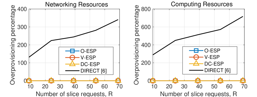
Figure 7. Over-provisioning of networking and computational resources of Sl-EDGE and DIRECT (Liu and Han, 2019).

Moreover, DIRECT does not explicitly slice storage resources. Thus, to perform a fair comparison, we consider the case where tenants do not request any storage resource. Let $D_{c}=75$ be the total number of edge nodes in the network. We let tenants randomly generate slice requests to obtain networking and computational resources. Results are shown in Fig. 7, where any positive value indicates resource over-provisioning.

Fig. 7 shows that Sl-EDGE never produces over-provisioning slices. Conversely, since DIRECT does not account for coupling among heterogeneous resources on the same edge node, it always incurs in over-provisioning, allocating up to 6x more resources than the available ones. These results conclude that already existing solutions, which perform well in 5G systems with networking and MEC functionalities decoupled at different points of the network, cannot be readily applied to scenarios where resources are simultaneously handled by edge nodes—which strongly motivates the need for approaches such as Sl-EDGE.

7.2. Maximizing the number of admitted slices

Let us now focus on the scenario where the IP owning the infrastructure aims at maximizing the number of slice requests admitted by Sl-EDGE—to maximize resource utilization, for instance. Although each slice request $r$ comes with an associated (monetary) value $v_{r}>0$, the above can be achieved by resetting the value of each request to $v_{r}=1$ in Problem (ESP).

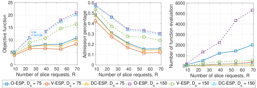
Figure 8. Sl-EDGE performance when maximizing the number of admitted slice requests.

Fig. 8 reports the performance of Sl-EDGE as a function of the total number $R$ of generated slice requests for different values of the number of edge nodes $D_{c}$. We notice that the number of admitted slices increase as the slice requests that are submitted to Sl-EDGE increase (left-side plot). However, Fig. 8 (center) clearly shows that the percentage of admitted slices rapidly decreases as $R$ increases (only $10$ requests are admitted by O-ESP when $D_{c}=75$ and $R=70$). This is due to the scarcity of resources at edge nodes, which prevents the admission of a large number of slices. Thus, IPs should either provide edge nodes with more resources, or increase the number of deployed edge nodes. Fig. 8 (left), indeed, shows that denser deployments of edge nodes (i.e., $D_{c}=150$) allows more slices to coexist on the same infrastructure.

Finally, the right-hand side plot of Fig. 8 shows the computational complexity of the three algorithms measured as the number of function evaluations needed to output a solution. As expected, the complexity of all algorithms increases as both $R$ and $D_{c}$ increase. Moreover, O-ESP, a fully centralized algorithm, has the highest computational complexity. V-ESP and DC-ESP, reduced-complexity versions of O-ESP, instead show lower complexity. However, V-ESP and DC-ESP admit approximately $10\%$ and $16\%$ less requests than O-ESP, respectively, due to their non-optimality.

7.3. Maximizing the profit of the IP

Let us now consider the case of slice admission and instantiation for profit maximization (Fig. 9). In this case, Sl-EDGE selects the slice requests to be admitted to maximize the total (monetary) value of the admitted slices. Similarly to Fig. 8, Fig. 9 (center) shows that increasing $R$ reduces the percentage of admitted slices.

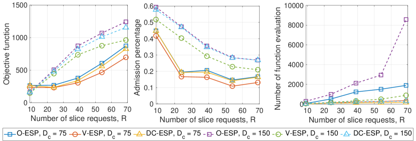
Figure 9. Sl-EDGE performance maximizing the profit of the IP.

Figure 10. Computational complexity of the proposed algorithms as a function of the similarity parameter $\epsilon$.

When compared to the problem described in Section 7.2, this profit maximization problem differs because (i) even if the number of edge nodes is small (i.e., $D_{c}=75$), profit maximization produces profits that rapidly increase with $R$, and (ii) the percentage of admitted requests steeply decreases as $R$ increases. Indeed, the higher the number of requests, the higher the probability that slices with high value are submitted by tenants. In this case, Sl-EDGE prioritizes more valuable requests at the expenses of others.

7.4. Impact of $\epsilon$ on the V-ESP algorithm

Finally, we investigate the impact of different choices on the performance of the V-ESP algorithm. Recall that $\epsilon$ regulates the number of edge nodes that are aggregated into virtual edge nodes (Section 6.1). The higher the value of $\epsilon$, the higher the percentage of edge nodes that are aggregated, and the smaller the number of virtual edge nodes generated by Sl-EDGE.

Fig. 10 shows the computational complexity of V-ESP as a function of $\epsilon$ for different number $D_{c}$ of deployed edge nodes. As expected, $\epsilon$ does not impact neither O-ESP nor DC-ESP, however the impact on V-ESP is substantial. Indeed, larger values of $\epsilon$ reduce the number of physical edge nodes in the network, which are instead substituted by virtual edge nodes (one per aggregated group). This reduction eventually results in decreased computational complexity. Surprisingly, Fig. 10 also shows that V-ESP enjoys an even lower computational complexity than that of the distributed DC-ESP when $\epsilon\approx 1$. Recall that V-ESP centrally determines an efficient slicing strategy over virtualized edge nodes, and these strategies are successively enforced by each cluster. This means that V-ESP can compute an efficient slicing policy as rapidly as DC-ESP while avoiding any coordination among different clusters. Overall, Fig. 10 shows that V-ESP (green dashed line) computes a solution 7.5x faster than O-ESP (purple dashed line) when $\epsilon$ is high.

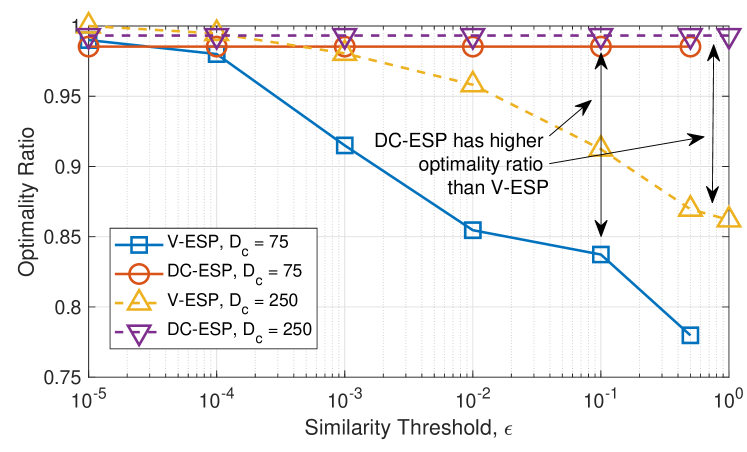
Figure 11. Optimality ratio of the algorithms proposed in Section 6 as a function of the similarity parameter $\epsilon$.

However, Fig. 11 shows that reduced computation complexity comes at the expense of efficiency.

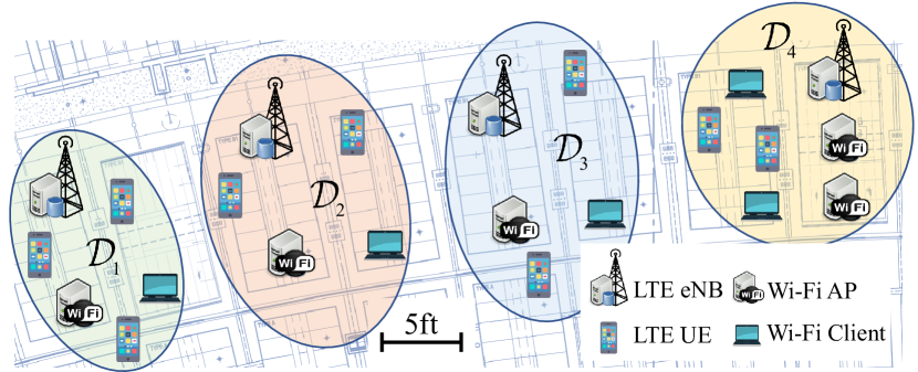
Figure 12. Sl-EDGE testbed configuration.

Indeed, the optimality ratio (i.e., the distance of the output of any approximation algorithm from the optimal solution of the problem) decreases as $\epsilon$ increases up to a maximum of 25% loss with respect to the optimal. Although the optimality ratio for $\epsilon=0.1$ is high (i.e., $92\%$ and $84\%$ for $D_{c}=75$ and $D_{c}=250$, respectively), clearly a trade-off between computational complexity and efficacy should be considered.

8. Sl-EDGE prototype

We prototyped Sl-EDGE on Arena, a large-scale 64-antennas SDR testbed (Bertizzolo et al., 2019). A server rack composed of 12 Dell PowerEdge R340 servers is used to control the testbed SDRs, and to perform baseband signal processing as well as generic computation and storage operations. The servers connect to a radio rack formed of 24 Ettus Research SDRs (16 USRPs N210 and 8 USRPs X310) through $10\>\mathrm{Gbit/s}$ optical fiber cables to enable low-latency and reactive communication with the radios. These are connected to 64 omnidirectional antennas through $100\>\mathrm{ft}$ coaxial cables. Antennas are hung off the ceiling of a $2240\>\mathrm{ft^{2}}$ office space and operate in the 2.4-2.5 and 4.9-5.9 GHz frequency bands. The USRPs in the radio rack achieve symbol-level synchronization through four OctoClock clock distributors.

We leveraged 14 USRPs of the above-mentioned testbed (10 USRPs N210 and 4 USRPs X310) to prototype Sl-EDGE. In our testbed, an edge node consists of one USRP and one server, the former provides networking capabilities, while the latter provides storage and computing resources. The testbed configuration adopted to prototype and evaluate Sl-EDGE performance is shown in Fig. 12.

Since there are no open-source experimental 5G implementations yet, we used the LTE-compliant srsLTE software (Gomez-Miguelez et al., 2016) to implement LTE networking slices. Since LTE and NR resource block grids are similar, we are confident that our findings remain valid for 5G scenarios. Specifically, srsLTE offers a standard-compliant implementation of the LTE protocol stack, including Evolved Packet Core and LTE base station (eNB) applications. We leveraged srsLTE to instantiate 4 eNBs on USRPs X310, while we employed 9 COTS cellular phones (Samsung Galaxy S5) as users. Each user downloads a data file from one of the rack servers, which are used as caching nodes with storage capabilities.

We consider three tenants demanding an equal number of LTE network slices (i.e., $\mbox{LS}_{1}$, $\mbox{LS}_{2}$ and $\mbox{LS}_{3}$) at times $t_{0}=0\>\mathrm{s}$, $t_{1}=40\>\mathrm{s}$, and $t_{2}=80\>\mathrm{s}$. Each tenant controls a single slice only and serves a set of UEs located in different clusters as shown in Table 1 (right).

Table 1. Per-cluster admitted RBs in $\mbox{LS}_{1}$, and UE association.

	$t_{0}\!=\![0,40]\mathrm{s}$	$t_{1}\!=\![40,80]\mathrm{s}$	$t_{2}\!=\![80,160]\mathrm{s}$		$\mbox{LS}_{1}$	$\mbox{LS}_{2}$	$\mbox{LS}_{3}$
$\mathcal{D}_{1}$	24	0	0		$\mbox{UE}_{1}$	$\mbox{UE}_{2}$	$\mbox{UE}_{7}$
$\mathcal{D}_{2}$	0	0	0		-	$\mbox{UE}_{3}$	$\mbox{UE}_{8}$
$\mathcal{D}_{3}$	24	24	0		$\mbox{UE}_{4}$	$\mbox{UE}_{5}$	$\mbox{UE}_{9}$
$\mathcal{D}_{4}$	42	24	0		$\mbox{UE}_{6}$	-	-

To test Sl-EDGE abilities in handling slices involving both networking and computation capabilities, we also implemented a video streaming slice where edge nodes stream a video file stored on an Apache instance through the dash.js reference player (DASH Industry Forum, 2019) running on the Chrome web browser. DASH allows real-time adaptation of the video bitrate, according to the client requests and the available resources (Stockhammer, 2011). Each streaming video was sent to the receiving server of the rack through USRPs N210 acting as SDR-based WiFi transceivers (WiFi Access Points (APs) and Clients in Fig. 12), using the GNU Radio-based IEEE 802.11a/g/p implementation (Bloessl et al., 2018). In the meanwhile, the edge node performed transcoding of video chunks using ffmpeg (FFmpeg Developers, 2019). We point out that each SDR can play multiple roles in the cluster (e.g., USRPs X310 can act as WiFi transceiver/LTE eNB), and the actual role is determined at run-time based on the slice types allocated to each tenant.

A demonstration of the operations of Sl-EDGE in the scenario of Fig. 12 is shown in Figs. 13, 14 and 15. Overall, the prototype of Sl-EDGE allocates and supports 11 heterogeneous slices simultaneously: 3 for cellular connectivity, 3 for video streaming over WiFi, and 5 for computation with the ffmpeg transcoding. Bitrate results for the LTE slices and individual UEs are reported in Fig. 13, where we show that Sl-EDGE provides an overall instantaneous throughput of $37~{}\mathrm{Mbit/s}$.

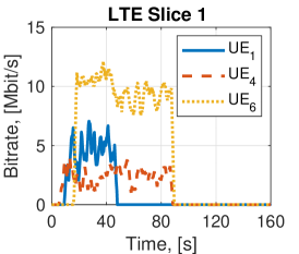
(a)

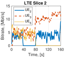
(b)

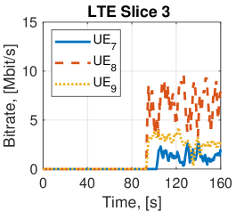
(c)

Figure 13. Instantiation of LTE network slices.

It is worth to point out that the throughput of each LTE slice, and thus each UE, varies according to the amount of resources allocated to the tenants. An example is shown in Table 1 (left), where we report the output of Sl-EDGE O-ESP algorithm (i.e., the amount of RBs allocated to LTE Slice 1 ($\mbox{LS}_{1}$)) in each cluster. Such an allocation impacts the throughput of UEs attached to slice $\mbox{LS}_{1}$. As an example, in Fig. 13 we notice that $\mathrm{UE}_{6}\in\mathcal{D}_{4}$ is allocated 42 RBs at $t_{0}$, 24 RBs in $t_{1}$, and 0 RBs in $t_{2}$ and approximately achieves a throughput of $12\mathrm{Mbit/s}$, $8\mathrm{Mbit/s}$ and $0\mathrm{Mbit/s}$, respectively.

The video streaming application from Fig. 14 involves 5 tenants that share 3 non-overlapping channels, allocated in any cluster $\mathcal{D}_{i},i\in\{1,2,3,4\}$. To avoid co-channel interference, Sl-EDGE only admits 3 flows at any given time. As Fig. 14 shows, during the first 70 seconds of the experiment only the slices for tenants 1, 2 and 3 are admitted, while tenant 4 needs to wait for tenant 3 to stop the video streaming before being granted a slice. Similarly, the slice for tenant 5 starts at time $t=140\>\mathrm{s}$, when the flow of tenant 1 stops. Meanwhile, the tenants submit requests for computation slices to transcode the videos with ffmpeg, which compete with srsLTE and GNU Radio slices necessary for LTE connectivity and video streaming in the 3 LTE eNBs and 5 WiFi APs of the 4 clusters. Moreover. in each server one of the 6 cores is reserved to the operating system exclusively and is never allocated to tenants. Fig. 15 shows that Sl-EDGE limits the total CPU utilization to 83%, which demonstrates that Sl-EDGE avoids over-provisioning of available resources.

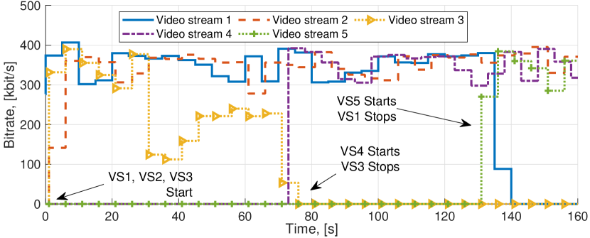
Figure 14. Dynamic instantiation of video streaming slices.

Figure 15. CPU utilization for networking and transcoding services.

9. Conclusions

In this paper, we have presented Sl-EDGE, a unified MEC slicing framework that instantiates heterogeneous slice services (e.g., video streaming, caching, 5G network access) on edge devices. We have first shown that the problem of optimally instantiating joint network-MEC slices is NP-hard. Then, we have proposed distributed algorithms that leverage similarities among edge nodes and resource virtualization to instantiate heterogeneous slices faster and within a short distance from the optimum. We have assessed the performance of our algorithms through extensive numerical analysis and on a 64-antenna testbed with 24 software-defined radios. Results have shown that Sl-EDGE instantiates slices 6x more efficiently then state-of-the-art MEC slicing algorithms, and that Sl-EDGE provides at once highly-efficient slicing of joint LTE connectivity, video streaming over WiFi, and ffmpeg video transcoding.

- (1)
- Afolabi et al. (2018) I. Afolabi, T. Taleb, K. Samdanis, A. Ksentini, and H. Flinck. 2018. Network slicing and softwarization: A survey on principles, enabling technologies, and solutions. IEEE Communications Surveys & Tutorials 20, 3 (Mar. 2018), 2429–2453.
- Agarwal et al. (2018) S. Agarwal, F. Malandrino, C.-F. Chiasserini, and S. De. 2018. Joint VNF placement and CPU allocation in 5G. In Proc. of IEEE INFOCOM. Honolulu, HI, USA.
- Al-Shuwaili and Simeone (2017) A. Al-Shuwaili and O. Simeone. 2017. Energy-efficient resource allocation for mobile edge computing-based augmented reality applications. IEEE Wireless Communications Letters 6, 3 (June 2017), 398–401.
- Bertizzolo et al. (2019) L. Bertizzolo, L. Bonati, E. Demirors, and T. Melodia. 2019. Arena: A 64-antenna SDR-based Ceiling Grid Testbed for Sub-6 GHz Radio Spectrum Research. In Proc. of ACM WiNTECH. Los Cabos, Mexico.
- Bizanis and Kuipers (2016) Nikos Bizanis and Fernando A Kuipers. 2016. SDN and virtualization solutions for the Internet of Things: A survey. IEEE Access 4 (2016), 5591–5606.
- Bloessl et al. (2018) B. Bloessl, M. Segata, C. Sommer, and F. Dressler. 2018. Performance Assessment of IEEE 802.11p with an Open Source SDR-based Prototype. IEEE Trans. on Mobile Computing 17, 5 (May 2018), 1162–1175.
- Bouet and Conan (2018) M. Bouet and V. Conan. 2018. Mobile edge computing resources optimization: A geo-clustering approach. IEEE Trans. on Network and Service Management 15, 2 (June 2018), 787–796.
- Boyd et al. (2011) S. Boyd, N. Parikh, E. Chu, B. Peleato, and J. Eckstein. 2011. Distributed optimization and statistical learning via the alternating direction method of multipliers. Now Foundations and Trends.
- Caballero et al. (2017) P. Caballero, A. Banchs, G. de Veciana, and X. Costa-Pérez. 2017. Network slicing games: Enabling customization in multi-tenant networks. In Proc. of IEEE INFOCOM. Atlanta, GA, USA.
- Castellano et al. (2019) G. Castellano, F. Esposito, and F. Risso. 2019. A Distributed Orchestration Algorithm for Edge Computing Resources with Guarantees. In Proc. of IEEE INFOCOM. Paris, France.
- DASH Industry Forum (2019) DASH Industry Forum. 2019. dash.js. https://tinyurl.com/ojd2bba.
- D’Oro et al. (2020) S. D’Oro, F. Restuccia, and T. Melodia. 2020. Toward Operator-to-Waveform 5G Radio Access Network Slicing. IEEE Communications Magazine 58, 4 (April 2020), 18–23. https://doi.org/10.1109/MCOM.001.1900316
- D’Oro et al. (2018) S. D’Oro, F. Restuccia, T. Melodia, and S. Palazzo. 2018. Low-complexity distributed radio access network slicing: Algorithms and experimental results. IEEE/ACM Trans. on Networking 26, 6 (Dec. 2018), 2815–2828.
- D’Oro et al. (2019) Salvatore D’Oro, F. Restuccia, A. Talamonti, and T. Melodia. 2019. The Slice Is Served: Enforcing Radio Access Network Slicing in Virtualized 5G Systems. In Proc. of IEEE INFOCOM 2019. Paris, France.
- Elf et al. (2001) Matthias Elf, C. Gutwenger, M. Jünger, and G. Rinaldi. 2001. Branch-and-Cut Algorithms for Combinatorial Optimization and Their Implementation in ABACUS. Springer Berlin Heidelberg, 157–222.
- Erol-Kantarci and Sukhmani (2018) M. Erol-Kantarci and S. Sukhmani. 2018. Caching and computing at the edge for mobile augmented reality and virtual reality (AR/VR) in 5G. In Ad Hoc Networks. Springer, 169–177.
- ETSI (2018a) ETSI. 2018a. 5G End to End Key Performance Indicators (KPI). https://tinyurl.com/ETSIStandard.
- ETSI (2018b) ETSI. 2018b. MEC in 5G networks. https://www.etsi.org/images/files/ETSIWhitePapers/etsi_wp28_mec_in_5G_FINAL.pdf.
- ETSI (2019a) ETSI. 2019a. MEC Deployments in 4G and Evolution Towards 5G. https://www.etsi.org/images/files/ETSIWhitePapers/etsi_wp24_MEC_deployment_in_4G_5G_FINAL.pdf.
- ETSI (2019b) ETSI. 2019b. MEC support for network slicing. https://portal.etsi.org/webapp/WorkProgram/Report_WorkItem.asp?WKI_ID=53580.
- FFmpeg Developers (2019) FFmpeg Developers. 2019. ffmpeg tool. http://ffmpeg.org/.
- Foukas et al. (2017) X. Foukas, M. K. Marina, and K. Kontovasilis. 2017. Orion: RAN slicing for a flexible and cost-effective multi-service mobile network architecture. In Proc. of ACM MobiCom. Snowbird, Utah, USA.
- Garcia-Aviles et al. (2018) G. Garcia-Aviles, M. Gramaglia, P. Serrano, and A. Banchs. 2018. POSENS: a practical open source solution for end-to-end network slicing. IEEE Wireless Communications 25, 5 (Oct. 2018), 30–37.
- Gomez-Miguelez et al. (2016) I. Gomez-Miguelez, A. Garcia-Saavedra, P.D. Sutton, P. Serrano, C. Cano, and D.J. Leith. 2016. srsLTE: An Open-source Platform for LTE Evolution and Experimentation. In Proc. of ACM WiNTECH. New York City, NY, USA.
- Gudipati et al. (2013) A. Gudipati, D. Perry, L. E. Li, and S. Katti. 2013. SoftRAN: Software defined radio access network. In Proc. of ACM HotSDN. Hong Kong, China.
- Halabian (2019) H. Halabian. 2019. Distributed resource allocation optimization in 5G virtualized networks. IEEE JSAC 37, 3 (Mar. 2019), 627–642.
- Han et al. (2019) B. Han, V. Sciancalepore, D. Feng, X. Costa-Perez, and H. D. Schotten. 2019. A Utility-Driven Multi-Queue Admission Control Solution for Network Slicing. In Proc. of IEEE INFOCOM. Paris, France.
- He et al. (2019) S. He, J. Ren, J. Wang, Y. Huang, Y. Zhang, W. Zhuang, and S. Shen. 2019. Cloud-Edge Coordinated Processing: Low-Latency Multicasting Transmission. IEEE JSAC 37, 5 (May 2019), 1144–1158.
- Hoang et al. (2018) D. T. Hoang, D. Niyato, D. N. Nguyen, E. Dutkiewicz, P. Wang, and Z. Han. 2018. A Dynamic Edge Caching Framework for Mobile 5G Networks. IEEE Wireless Communications 25, 5 (Oct. 2018), 95–103.
- Holma and Toskala (2009) H. Holma and A. Toskala. 2009. LTE for UMTS: OFDMA and SC-FDMA Based Radio Access. Wiley.
- Huang (2008) A. Huang. 2008. Similarity measures for text document clustering. In Proc. of the NZCSRSC. Christchurch, New Zealand.
- Jiang et al. (2017) M. Jiang, M. Condoluci, and T. Mahmoodi. 2017. Network slicing in 5G: An auction-based model. In Proc. of IEEE ICC. Paris, France.
- Kaloxylos (2018) A. Kaloxylos. 2018. A survey and an analysis of network slicing in 5G networks. IEEE Communications Standards Magazine 2, 1 (Mar. 2018), 60–65.
- Lin et al. (2013) M.-H. Lin, J. G. Carlsson, D. Ge, J. Shi, and J.-F. Tsai. 2013. A review of piecewise linearization methods. Hindawi Mathematical Problems in Engineering (2013).
- Liu et al. (2016) J. Liu, Y. Mao, J. Zhang, and K. B. Letaief. 2016. Delay-optimal computation task scheduling for mobile-edge computing systems. In Proc. of IEEE ISIT. Barcelona, Spain.
- Liu and Han (2019) Q. Liu and T. Han. 2019. DIRECT: Distributed Cross-Domain Resource Orchestration in Cellular Edge Computing. In Proc. of ACM MobiHoc. Catania, Italy.
- Mach and Becvar (2017) P. Mach and Z. Becvar. 2017. Mobile edge computing: A survey on architecture and computation offloading. IEEE Communications Surveys & Tutorials 19, 3 (Mar. 2017), 1628–1656.
- Mancuso et al. (2019) V. Mancuso, P. Castagno, M. Sereno, and M. A. Marsan. 2019. Slicing Cell Resources: The Case of HTC and MTC Coexistence. In Proc. of IEEE INFOCOM 2019. Paris, France.
- Mandelli et al. (2019) S. Mandelli, M. Andrews, S. Borst, and S. Klein. 2019. Satisfying Network Slicing Constraints via 5G MAC Scheduling. In Proc. of IEEE INFOCOM 2019. Paris, France.
- Mao et al. (2017) Y. Mao, C. You, J. Zhang, K. Huang, and K. B. Letaief. 2017. A survey on mobile edge computing: The communication perspective. IEEE Communications Surveys & Tutorials 19, 4 (Aug. 2017).
- Misra and Saha (2019) S. Misra and N. Saha. 2019. Detour: Dynamic Task Offloading in Software-Defined Fog for IoT Applications. IEEE JSAC 37, 5 (May 2019), 1159–1166.
- Miyazaki et al. (2015) S. Miyazaki, N. Morimoto, and Y. Okabe. 2015. Approximability of Two Variants of Multiple Knapsack Problems. In Proc. of Springer Intl. Conference on Algorithms and Complexity. Cham, Switzerland.
- Ndikumana et al. (2019) A. Ndikumana, N. H. Tran, T. M. Ho, Z. Han, W. Saad, D. Niyato, and C. S. Hong. 2019. Joint communication, computation, caching, and control in big data multi-access edge computing. IEEE Trans. on Mobile Computing (Mar. 2019).
- Rost et al. (2017) P. Rost, C. Mannweiler, D. S. Michalopoulos, C. Sartori, V. Sciancalepore, N. Sastry, O. Holland, S. Tayade, B. Han, D. Bega, D. Aziz, and H. Bakker. 2017. Network slicing to enable scalability and flexibility in 5G mobile networks. IEEE Communications Magazine 55, 5 (May 2017), 72–79.
- Shi et al. (2014) W. Shi, Q. Ling, K. Yuan, G. Wu, and W. Yin. 2014. On the linear convergence of the ADMM in decentralized consensus optimization. IEEE Trans. on Signal Processing 62, 7 (Apr. 2014), 1750–1761.
- Stockhammer (2011) T. Stockhammer. 2011. Dynamic Adaptive Streaming over HTTP: Standards and Design Principles. In Proc. of ACM MMSys. San Jose, CA, USA.
- Sun et al. (2019) Y. Sun, M. Peng, S. Mao, and S. Yan. 2019. Hierarchical radio resource allocation for network slicing in fog radio access networks. IEEE Trans. on Vehicular Technology 68, 4 (Apr. 2019), 3866–3881.
- Taleb et al. (2017) T. Taleb, K. Samdanis, B. Mada, H. Flinck, S. Dutta, and D. Sabella. 2017. On multi-access edge computing: A survey of the emerging 5G network edge cloud architecture and orchestration. IEEE Communications Surveys & Tutorials 19, 3 (May 2017), 1657–1681.
- Tang and He (2018) L. Tang and S. He. 2018. Multi-user computation offloading in mobile edge computing: A behavioral perspective. IEEE Network 32, 1 (Jan. 2018), 48–53.
- Tran and Pompili (2018) T. X. Tran and D. Pompili. 2018. Joint task offloading and resource allocation for multi-server mobile-edge computing networks. IEEE Trans. on Vehicular Technology 68, 1 (Jan. 2018), 856–868.
- Van Huynh et al. (2019) N. Van Huynh, D. Thai Hoang, D. N. Nguyen, and E. Dutkiewicz. 2019. Optimal and Fast Real-Time Resource Slicing With Deep Dueling Neural Networks. IEEE JSAC 37, 6 (June 2019), 1455–1470.
- Wang et al. (2019) J. Wang, J. Hu, G. Min, W. Zhan, Q. Ni, and N. Georgalas. 2019. Computation Offloading in Multi-Access Edge Computing Using a Deep Sequential Model Based on Reinforcement Learning. IEEE Communications Magazine 57, 5 (May 2019), 64–69.
- Xu and Wunsch (2005) R. Xu and D. C. Wunsch. 2005. Survey of clustering algorithms. IEEE Trans. on Neural Networks 16, 3 (May 2005), 645–678.
- Yang et al. (2018) S.-R. Yang, Y.-J. Tseng, C.-C. Huang, and W.-C. Lin. 2018. Multi-Access Edge Computing Enhanced Video Streaming: Proof-of-Concept Implementation and Prediction/QoE Models. IEEE Trans. on Vehicular Technology 68, 2 (Feb. 2018), 1888–1902.
- Zhang et al. (2018) K. Zhang, S. Leng, Y. He, S. Maharjan, and Y. Zhang. 2018. Cooperative content caching in 5G networks with mobile edge computing. IEEE Wireless Communications 25, 3 (June 2018), 80–87.
- Zhang et al. (2019) Q. Zhang, F. Liu, and C. Zeng. 2019. Adaptive interference-aware VNF placement for service-customized 5G network slices. In Proc. of IEEE INFOCOM 2019. Paris, France.