Space-Time Medium Functions as a Perfect Antenna-Mixer-Amplifier Transceiver

Abstract

We show that a space-time-varying medium can function as a front-end transceiver, i.e., an antenna-mixer-amplifier. Such a unique functionality is endowed by space-time surface waves associated with complex space-time wave vectors in a subluminal space-time medium. The proposed structure introduces pure frequency up- and down-conversions and with very weak undesired time harmonics. In contrast to other recently proposed space-time mixers, a large frequency up-/down conversion ratio, associated with gain is achievable. Furthermore, as the structure does not operate based on progressive energy transition between the space-time modulation and the incident wave, it possesses a subwavelength thickness (metasurface). Such a multi-functional, highly efficient and compact medium is expected to find various applications in modern wireless telecommunication systems.

I Introduction

Reception and transmission of electromagnetic waves is the essence of wireless telecommunications vannucci1995wireless ; saunders2007antennas . Such a task requires various functions, such as power amplification, frequency conversion, and wave radiation. These functions have been conventionally performed by electronic components and electromagnetic structures, such as transistor-based amplifiers, semiconductor-based diode mixers, and resonance-based antennas. The ever increasing demand for versatile wireless telecommunication systems has led to a substantial need in multi-functional components and compact integrated circuits. In general, each natural medium may introduce a single function, e.g., a resonator may operate as an antenna at a specific frequency. To contrast this conventional approach, a single medium exhibiting several functions concurrently could lead to a disruptive evolution in telecommunication technology.

Recently, space-time-modulated media have attracted a surge of scientific interest thanks to their capability in multifunctional operations, e.g., mixer-duplexer-antenna Taravati_LWA_2017 , unidirectional beam splitters Taravati_Kishk_PRB_2018 , nonreciprocal filters alvarez2019coupling ; wu2019isolating , and signal coding metagratings taravati_PRApp_2019 . In addition, a large number of versatile and high efficiency electromagnetic systems have been recently reported based on the unique properties of space-time modulation, including space-time metasurfaces for advanced wave engineering and extraordinary control over electromagnetic waves Fan_APL_2016 ; Fan_mats_2017 ; Salary_2018 ; salary2019dynamically ; Taravati_Kishk_TAP_2019 ; zang2019nonreciprocal_metas ; inampudi2019rigorous ; elnaggar2019generalized ; wang2018photonic ; Grbic2019serrodyne ; Taravati_Kishk_MicMag_2019 ; ptitcyn2019time ; sedehtopological ; du2019simulation ; wang2019multifunctional ; taravati2019full ; li2020time ; sedeh2020topological , nonreciprocal platforms Taravati_thesis ; wentz1966nonreciprocal ; Taravati_PRB_2017 ; Taravati_PRB_SB_2017 ; Taravati_PRAp_2018 ; oudich2019space ; chegnizadeh2020non , frequency converters Taravati_PRB_Mixer_2018 ; Grbic2019serrodyne , and time-modulated antennas shanks1961new ; Alu_PNAS_2016 ; ramaccia2018nonreciprocity ; taravati2018space ; salary2019nonreciprocal ; zang2019nonreciprocal . Such strong capability of space-time-modulated media is due to their unique interactions with the incident field Taravati_PRB_2017 ; li2019nonreciprocal ; correas2018magnetic ; liu2018huygens ; du2019simulation ; elnaggar2019modelling ; taravati2019_mix_ant .

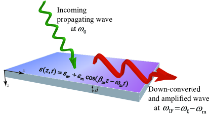
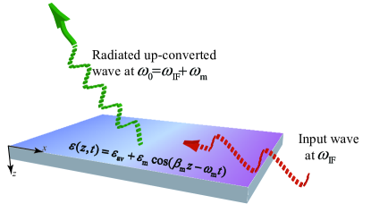
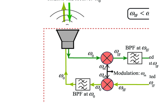
Figure 1: Functionality of the antenna-mixer-amplifier space-time surface wave medium. (a) Down-link (reception) state, where a strong transition between a space-wave at $\omega_{0}$ to a space-time surface wave at $\omega_{\text{IF}}=\omega_{0}-\omega_{\text{m}}$ occurs. (b) Up-link (transmission) state, where a transition between a space-time surface wave at $\omega_{\text{IF}}$ to a space-wave at $\omega_{\text{0}}=\omega_{\text{IF}}+\omega_{\text{m}}$ occurs. (c) Circuital representation of the combined antenna-mixer-amplifier space-wave medium in (a) and (b).

This paper reveals that a space-time medium can function as a full transceiver front-end, that is, an antenna-mixer-amplifier-filter system. Specific related contributions of this study are as follows.

• We show that the space-time medium operates as an antenna per se. Such an interesting functionality of the space-time medium is endowed by space-time surface waves. Other recently proposed space-time antenna systems are formed by integration of the space-time-modulated medium with an antenna Taravati_APS_2015 ; Alu_PNAS_2016 ; Taravati_LWA_2017 , and hence suffer from a number of drawbacks, i.e., requiring long structures, low efficiency and narrow-band operation.

• The proposed antenna-mixer-amplifier introduces large frequency up- and -down conversion ratios. This is very practical, because in real-scenario wireless telecommunication systems, a large frequency conversion is required, i.e., a frequency conversion from a microwave/millimeter-wave frequency to an intermediate frequency in receivers. In contrast, recently proposed space-time frequency converters suffer from very low frequency conversion ratios (up-/down-converted frequency is very closed to the input frequency) Taravati_APS_2015 ; Alu_PNAS_2016 ; Taravati_LWA_2017 ; Grbic2019serrodyne .

• Recently proposed space-time systems operate based on a progressive coupling between the incident wave and the space-time modulation Fan_NPH_2009 ; Fan_PRL_109_2012 ; Taravati_LWA_2017 ; Chamanara_PRB_2017 ; Taravati_PRB_Mixer_2018 , and hence a thick (compared to the wavelength) slab is required. In contrast, the proposed antenna-mixer-amplifier does not work based on progressive coupling between the incident wave and the space-time modulation and hence is formed by a thin (sub-wavelength) slab. As a result, the proposed structure is classified among metasurface categories and is compatible with the compactness requirements of modern wireless telecommunication systems.

• The proposed medium inherently operates as a band-pass filter, i.e., a pure frequency down- and up-conversions occurs so that the undesired time harmonics are highly suppressed. Such a property is governed by the subluminal operation of space-time modulation.

• In contrast to conventional mixers that introduce a significant conversion loss, here a conversion gain may be achieved in the down-link or up-link. In addition, the radiation from the antenna-mixer-amplifier is very directive.

The paper is organized as follows. Section II presents the operation principle of the antenna-mixer-amplifier. Then, Sec. III investigates the theoretical aspects of the work, and provides an analysis of the wave propagation in the antenna-mixer-amplifier space-time medium. Next, Sec. IV presents the design procedure of the structure, and gives an approximate closed-form solution to calculate the thickness and receive/transmit power gain of the structure. Section V gives the time and frequency domain numerical simulation results for the designed antenna-mixer-amplifier. Finally, Sec. VI concludes the paper.

II Operation Principle

Consider the antenna-mixer-amplifier slab in Fig. 1, with the thickness of $d$ and a spatiotemporally-periodic electric permittivity as

$$\epsilon(z,t)=\epsilon_{\text{av}}+\epsilon_{\text{m}}\cos(\beta_{\text{m}}z-\omega_{\text{m}}t),$$ (1)

with $\epsilon_{\text{av}}$ being the average electric permittivity of the background medium, and $\epsilon_{\text{m}}$ representing the modulation amplitude. In Eq. (1), $\omega_{\text{m}}$ denotes the temporal frequency of the modulation, and $\beta_{\text{m}}$ is the spatial frequency of the modulation represented by

$$\beta_{\text{m}}=\dfrac{\omega_{\text{m}}}{v_{\text{m}}}=\dfrac{\omega_{\text{m}}}{\varGamma v_{\text{b}}},$$ (2)

where $v_{\text{m}}$ and $v_{\text{b}}$ are the phase velocity of the modulation and the background medium, respectively, and $\varGamma=v_{\text{m}}/v_{\text{b}}$ is the space-time velocity ratio Taravati_PRB_2017 .

The slab in Fig. 1 is obliquely illuminated by a $y$-polarized incident electric filed under an angle of incidence of $\theta_{\text{i}}$, as

$$\mathbf{E}_{\text{i}}(x,z,t)=\mathbf{\hat{y}}E_{\text{i}}e^{i\left(k_{x}x+k_{z}z-\omega_{0}t\right)},$$ (3)

where $E_{\text{i}}$ is the amplitude of the incident wave, and $\omega_{0}$ and $k_{\text{0}}=\sqrt{k_{x}^{2}+k_{z}^{2}}=\sqrt{(k_{0}\sin(\theta_{\text{i}}))^{2}+(k_{0}\cos(\theta_{\text{i}}))^{2}}$ are respectively temporal and spatial frequencies of the incident wave. Here, $k_{0}=\omega_{0}/c$, with $c$ being the velocity of light in vacuum.

In the receiving state (down-link) in Fig. 1, strong transition between a space-wave, with temporal frequency $\omega_{0}$, to a space-time surface wave, with temporal frequency $\omega_{\text{IF}}=\omega_{0}-\omega_{\text{m}}$, occurs. In the transmission state (up-link) in Fig. 1 a transition between a space-time surface wave at $\omega_{\text{IF}}$ to a space-wave at $\omega_{\text{0}}=\omega_{\text{IF}}+\omega_{\text{m}}$ occurs.

Figure 1 shows an equivalent circuit representation of the antenna-mixer-amplifier in Figs. 1 and 1. Thanks to the unique properties of space-time-modulated media, that will be described later in this study, such a medium introduces the functionality of a highly directive antenna, a pure frequency up-converter, a pure frequency down-converter, up-link and down-link filters, and a down-link amplifier. Such a rich functionality has not been experienced in other media unless several components and media are integrated, as shown in Fig. 1. However, here we show that a single medium can offer such versatile and useful operation.

As the slab is periodic in both space and time, the spatial and temporal frequencies of the space-time harmonics inside the structure are governed by the momentum conservation law, i.e.,

$$\gamma_{z,n}=\beta_{z,0}+n\beta_{\text{m}}+i\alpha_{z,n},$$ (4a)

and the energy conservation law, i.e.,

$$\omega_{n}=\omega_{0}+n\omega_{\text{m}}.$$ (4b)

The scattering angles of the space-time harmonics in regions 1 and 3 (reflection to the top and transmission to the bottom of the medium, respectively) may be determined by the Helmholtz relations, i.e., $k_{0}^{2}\sin^{2}(\theta_{\text{i}})+k_{0,n}^{2}\cos^{2}(\theta_{\text{r}n})=k_{0,n}^{2}$ and $k_{0}^{2}\sin^{2}(\theta_{\text{i}})+k_{0,n}^{2}\cos^{2}(\theta_{\text{t}n})=k_{0,n}^{2}$, with $\theta_{\text{r}n}$ and $\theta_{\text{t}n}$ being the reflection and transmission angles of the $n^{\text{th}}$ space-time harmonics, reading taravati_PRApp_2019

$$\theta_{\text{r}n}=\theta_{\text{t},n}=\sin^{-1}\left(\frac{\sin(\theta_{\text{i}})}{1+n\omega_{\text{m}}/\omega_{0}}\right),$$ (5)

where $k_{0n}=\omega_{n}/c=(\omega_{0}+n\omega_{\text{m}})/c$. Therefore, given the common tangential wavenumber, $k_{x}=k_{0}\sin(\theta_{\text{i}})$ in all the regions, the reflection and transmission angles for the $n^{\text{th}}$ space-time harmonic are equal. Equation (5) shows that the harmonics in the $n$-interval $[\omega_{0}(\sin\theta_{\text{i}}-1)/\omega_{\text{m}},+\infty]$ are scattered at different angles ranging from $0$ to $\pi/2$ through $\theta_{\text{i}}$ for $n=0$. However, the space-time harmonics outside of this interval represent imaginary $k_{z,n}$ and hence propagate as space-time surface waves along the two boundaries of the slab at $z=0$ and $z=d$.

The scattering angles of the space-time harmonics inside the space-time-modulated medium read

$$\theta_{n}=\tan^{-1}\left(\frac{k_{x}}{\beta_{z,n}}\right)=\tan^{-1}\left(\frac{k_{0}\sin(\theta_{\text{i}})}{\beta_{z,0}+n\beta_{\text{m}}}\right).$$ (6)

Figure 2 shows the structure of the antenna-mixer-amplifier space-time medium. We aim to design the structure such that the first lower space-time harmonic, $n=-1$, outside the medium scatters along the boundary of the medium, i.e., $\theta_{\text{r},-1}=\theta_{\text{t},-1}=90^{\circ}$. Hence, using Eq. (5), the incident angle reads

$$\theta_{\text{i}}=\sin^{-1}\left(1-\frac{\omega_{\text{m}}}{\omega_{0}}\right).$$ (7)

In addition, to achieving a strong transition to the $n=-1$ harmonic, the scattered $n=-1$ harmonic inside the medium should propagate in parallel to the two space-time surface waves on the two boundaries of the medium at $z=0$ and $z=d$, i.e., $\theta_{n=-1}=90^{\circ}$. Thus, using Eq. (6), we achieve

$$\beta_{z,-1}=0.$$ (8)

As a result, the $z$ component of the Wave vector inside the medium is purely imaginary, i.e., $\gamma_{z,-1}=i\alpha_{z,-1}$, whereas the incident field wavenumber $k_{z}$ is purely real.

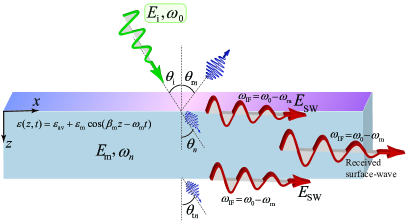
Figure 2: Operation principle of the antenna-mixer-amplifier space-time medium. Transition of the incident space-wave to space-time surface waves at the two boundaries of the medium ($\theta_{\text{r},-1}=\theta_{\text{t},-1}=90^{\circ}$) as well as inside it ($\theta_{-1}=90^{\circ}$)).

The space-time-modulated medium presents transition from the fundamental harmonic $n=0$ to a large (theoretically infinite, $-\infty<n<\infty$) number of space-time harmonics. Such a transition is very strong for the luminal space-time modulation, where the space-time modulation velocity is close to the background phase velocity, i.e., $v_{\text{m}}=v_{\text{b}}$ Taravati_PRB_2017 ; Taravati_PRAp_2018 .

To prevent generation of strong undesired time harmonics, here the space-time-modulated medium operates in the subluminal regime, where $0<v_{\text{m}}<v_{\text{b}}$, i.e.,

$$0<\varGamma_{\text{subluminal}}<\sqrt{\frac{\epsilon_{\text{r}}}{\epsilon_{\text{av}}+\epsilon_{\text{m}}}}.$$ (9)

As a result, a pure and precise transition between the fundamental ($n=0$) harmonic and the desired (here $n=-1$) space-time surface wave harmonic can occur.

III Theoretical investigation

III.1 Analytical solution

Considering the TE_y incident field in Eq. (3), the incident magnetic field reads

$$\begin{split}\mathbf{H}_{\text{i}}(x,z,t)&=\frac{1}{\eta_{1}}\left[\mathbf{\hat{k}}_{\text{i}}\times\mathbf{E}_{\text{i}}^{\text{F}}(x,z,t)\right]\\ &=\left[-\mathbf{\hat{x}}\cos(\theta_{\text{i}})+\mathbf{\hat{z}}\sin(\theta_{\text{i}})\right]\dfrac{E_{0}}{\eta_{1}}e^{i\left(k_{x}x+k_{z}z-\omega_{0}t\right)},\end{split}$$ (10)

where $\eta_{1}=\sqrt{\mu_{0}/\epsilon_{0}}$ is the characteristic impedance of free space. Since the space-time-modulated medium is periodic in space and time, the electric and magnetic fields in the slab may be decomposed to space-time Bloch-Floquet harmonics, as

$$\mathbf{E}_{\text{m}}(x,z,t)=\mathbf{\hat{y}}\sum_{n}\textbf{E}_{n}e^{i\gamma_{z,n}z}e^{i\left(k_{x}x-\omega_{n}t\right)},$$ (11a)

and

$$\begin{split}\mathbf{H}_{\text{m}}(x,z,t)=\dfrac{1}{k}\sum_{n}\textbf{H}_{n}\left[-\mathbf{\hat{x}}\beta_{z,n}+\mathbf{\hat{z}}k_{x}\right]e^{i\gamma_{z,n}z}e^{i\left(k_{x}x-\omega_{n}t\right)}.\end{split}$$ (11b)

The unknown coefficients in Eqs. (11a) and (11b), $\gamma_{z,n}=\beta_{z,n}+i\alpha_{z,n}$, $E_{n}$ and $H_{n}$ shall be found through the following procedure. We first construct and solve the corresponding wave equation. Next, we fix the source frequency $\omega_{0}$ and then find the corresponding discrete $\gamma_{z,n}$ solutions, which form the dispersion diagram of the space-time medium. We next apply the spatial boundary conditions at the edges of the slab, i.e. at $z=0$ and $z=d$, for all the $(\omega_{0},\gamma_{z,n})$ states in the dispersion diagram. This provides the unknown field coefficients $E_{n}$ and $H_{n}$ inside the slab, as well as the scattered (reflected and transmitted) fields outside the slab, i.e., $E_{\text{R}}$ and $E_{\text{T}}$.

The homogeneous wave equation reads

$$\nabla^{2}\mathbf{E}_{\text{m}}(x,z,t)-\frac{1}{{{c^{2}}}}\frac{{{\partial^{2}}\left[\epsilon(z,t)\mathbf{E}_{\text{m}}(x,z,t)\right]}}{{\partial{t^{2}}}}=0.$$ (12)

Inserting (11a) and (1) into (12), and using the Fourier series expansion for the permittivity, results in

$$E_{n}\left[\frac{k_{x}^{2}+(\beta_{z,n}+i\alpha_{z,n})^{2}}{\left[(\omega_{0}+n\omega_{\text{m}})/c\right]^{2}}\right]-\sum\limits_{k=-\infty}^{\infty}\tilde{\epsilon}_{k}E_{n-k}=0.$$ (13)

where $\tilde{\epsilon}_{k}$ are the Fourier series coefficients of the permittivity. Equation (13) may be cast to the matrix form as

$$[K]\cdot[E_{n}]=0,$$ (14)

where $[K]$ is the $(2N+1)\times(2N+1)$ matrix with elements

$$\begin{split}K_{nn}&=\left[\frac{k_{x}^{2}+(\beta_{z,n}+i\alpha_{z,n})^{2}}{\left[(\omega_{0}+n\omega_{\text{m}})/c\right]^{2}}\right]-\epsilon_{0},\\ K_{nk}&=-\tilde{\epsilon}_{n-k},\quad\text{for }n\neq k,\end{split}$$ (15)

where $2N+1$ is the number of truncated harmonics. Then, the dispersion relation reads

$$\text{det}\left\{[K]\right\}=0,$$ (16)

Once the dispersion diagram is formed, for a given incident temporal frequency $\omega_{0}$, the corresponding wave number, i.e., $\gamma_{z,n}$, inside the slab can be computed. Next, the unknown field amplitudes $E_{n}$ in the slab are found by solving (14) after determining the $E_{0}$ satisfying boundary conditions. Figure 3 shows a qualitative 3D dispersion diagram of a subluminal space-time modulated medium, composed of an infinite periodic set of double-cones with apexes at $\beta_{z,0}=-n\beta_{\text{m}}$ and $k_{x}=0$ and the slope $\varGamma$. As the slope $\varGamma$ increases and goes towards unity, the cones get closer to each other and start touching other cones(harmonics). As a result, stronger transition between harmonics occurs and yields transitions of the power from the fundamental harmonic to a large number of harmonics. However, this is not what we aim at. As we are interested in a pure transition to a desired harmonic ($n=-1$), we require a subluminal space-time modulation defined in Eq. (9).

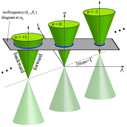
Figure 3: 3D-dispersion diagram of the space-time medium, formed by an infinite number of double cones each of which representing a space-time harmonic.

Figure 4 plots the analytical isofrequency dispersion diagram, computed using (16), for the subluminal regime where $\varGamma=0.2$. We have chosen a specific $\theta_{\text{i}}$, where the $n=-1$ harmonic is excited at a point corresponding to $\beta_{z,-1}=0$ (i.e., $\beta_{z,0}/\beta_{\text{m}}=+1$). As a consequence, the $n=-1$ harmonic scatters along the $x$-direction, i.e., $\theta_{\text{r},-1}=90^{\circ}$. Although the real part of the $z$ component of the wavevector of the $n=-1$ harmonic is zero ($\beta_{z,-1}=0$), its imaginary part is greater than zero, and hence $\gamma_{z,-1}=i\alpha_{z,-1}$.

Figure 4 shows that the transition between the forward $n=0$ and $n=-1$ harmonics (highlighted with magenta arrows) occurs for both reception (down-link) and transmission (up-link). This may as well be verified by Eq. (6) as follows. For the down-link, the incident wave ($n=0$) with the incident angle of $\theta_{\text{i}}^{\text{RX}}$ and wavenumber of $\beta_{z,0}^{\text{RX}}=\beta_{\text{m}}$ makes a transition to the down-converted harmonic ($n=-1$), which is attributed to $\theta_{\text{-1}}^{\text{RX}}=90^{\circ}$, $\beta_{z,-1}^{\text{RX}}=0$ and $\gamma_{z,-1}^{\text{RX}}=i\alpha_{z,-1}^{\text{RX}}$. However, for the up-link (transmission state), the incident wave ($n=0$) with the incident angle of $\theta_{\text{i}}^{\text{TX}}=90^{\circ}$ and wavenumber of $\beta_{z,0}^{\text{TX}}=0$ makes a transition to the up-converted harmonic ($n=+1$) with $\theta_{\text{+1}}^{\text{TX}}=\theta_{\text{0}}^{\text{RX}}=\theta_{\text{i}}^{\text{RX}}$, which is attributed to $\beta_{z,+1}^{\text{TX}}=\beta_{\text{m}}$ and $\gamma_{z,+1}^{\text{TX}}=\beta_{\text{m}}$.

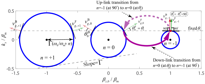
Figure 4: Analytical isofrequency dispersion diagram for $\varGamma=0.2$ and $\epsilon_{\text{m}}=\rightarrow 0$, showing down-link (reception) and up-link (transmission) electromagnetic transitions between the fundamental propagating harmonic ($n=0$) and the space-time surface wave harmonic ($n=-1$). Excitation of the medium at $\theta_{\text{i}}$ leads to excitation of the $n=-1$ at $90^{\circ}$.

IV Design Procedure

IV.1 Complex Dispersion Diagrams

Figure 5 plots the analytical isofrequency dispersion diagram ($\beta_{z,n}(k_{x})$ at $\omega/\omega_{\text{m}}=1.363$) of the sinusoidally space-time surface wave medium with the electric permittivity in (1) for the subluminal regime, i.e., $\varGamma=0.55$ for $\epsilon_{\text{m}}\rightarrow 0$. It may be seen from this figure that forward $n=0$ and $n=-1$ harmonics are excited very close to each other, where $n=0$ is excited at an angle of scattering of $\theta_{0}=\theta_{\text{i}}=15^{\circ}$. However, the $n=-1$ harmonic is intentionally excited at the angle of scattering of $\theta_{-1}=90^{\circ}$.

Figure 5 plots the same isofrequency $\beta_{z,n}(k_{x})$ diagram as Figure 5 except for a greater modulation amplitude of $\epsilon_{\text{m}}=0.45$. As a result of non-equilibrium in the electric and magnetic permitivitties of the medium, several electromagnetic badgaps appear at the intersections between space-time harmonics Taravati_PRAp_2018 . As a consequence, strong coupling between some of the harmonics has occurred, e.g. between the $n=0$ and $n=-1$ harmonics.

Figure 5 plots the complex isofrequency dispersion diagram $\gamma_{z,n}(k_{x})$ for the medium in Fig. 5. This diagram is formed by two different curves, i.e., the real $\beta_{z,n}(k_{x})$ and the imaginary $\alpha_{z,n}(k_{x})$ parts of the wavenumber. For the sake of clarification, we have included only a few number of harmonics. This figure shows that at the excited angle of incidence $\theta_{\text{i}}=15^{\circ}$, the $n=0$ harmonic introduces a pure real wavenumber, i.e., $\gamma_{z,0}=\beta_{z,0}$, whereas the $n=-1$ harmonic acquires a pure imaginary wavenumber, that is, $\gamma_{z,-1}=i\alpha_{z,-1}$. As a result, a perfect space-time transition from a pure propagating wave to a pure space-time surface wave is ensured.

Figure 5 plots the complex dispersion diagram, i.e., $\gamma_{z,n}(\omega_{0})$ for the medium in Fig. 5 and 5. This figure shows the strong transition between $n=0$ and $n=-1$ harmonics from the $k_{x}=0.218$ (corresponding to $\theta_{\text{i}}=15^{\circ}$) cut.

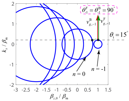
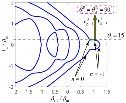
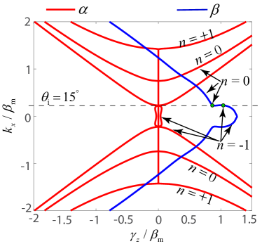
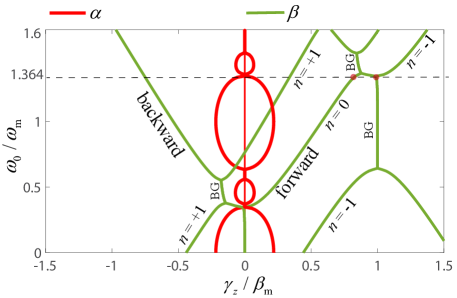
Figure 5: Analytical dispersion diagram of the sinusoidally space-time surface wave medium with the electric permittivity in (1) for subluminal regime, i.e., $\varGamma=0.55$. (a) Isofrequency diagram, i.e., $\beta_{z,n}(k_{x})$ at $\omega/\omega_{\text{m}}=1.363$, and for $\epsilon_{\text{m}}\rightarrow 0$. (b) Same as (a) except for greater modulation amplitude $\epsilon_{\text{m}}=0.45$. (c) Isofrequency diagram of the medium in (b), which includes the real and imaginary parts of the $\gamma_{z,n}$, i.e., $\beta_{z,n}$ and $\alpha_{z,n}$, for $n=0$ and $n=-1$. (d) Dispersion diagram, i.e., $\gamma_{z,n}(\omega_{0})$ for the medium in (a) and (b) for the $k_{x}=0.218$ (corresponding to $\theta_{\text{i}}=15^{\circ}$) cut.

IV.2 Approximate closed-form solution

To best investigate the efficiency of the antenna-mixer-amplifier, we present an approximate closed-form solution. Such an approximate closed-form solution clearly shows the effect of modulation parameters on the efficiency of the proposed antenna-mixer-amplifier medium.

IV.2.1 Reception state (down-link)

Equations (S7) and (S9) in the supplemental material form a matrix differential equation. For the down-link, the initial conditions of $E_{0}(0)=E_{\text{i}}$ and $E_{-1}(0)=0$ gives

$$E_{0}(z)=E_{\text{i}}\cos\left(\dfrac{\epsilon_{\text{m}}k_{0}k_{-1}}{4\sqrt{\gamma_{z,-1}\gamma_{z,0}}}z\right),$$ (17)

$$E_{-1}(z)=iE_{\text{i}}\dfrac{k_{-1}}{k_{0}}\sqrt{\dfrac{\gamma_{z,0}}{\gamma_{z,-1}}}\sin\left(\dfrac{\epsilon_{\text{m}}k_{0}k_{-1}}{4\sqrt{\gamma_{z,-1}\gamma_{z,0}}}z\right),$$ (18)

where $k_{-1}=\omega_{-1}/c^{2}$. The optimal transition from the incident field to the space-time surface wave occurs at $z=d$, where

$$\frac{d}{dz}E_{-1}(z)|_{z=d}=0,$$ (19)

yielding $|\epsilon_{\text{m}}k_{0}k_{-1}d/(4\sqrt{\gamma_{z,-1}\gamma_{z,0}})|=\pi/2$ which corresponds to

$$d=2\pi\left|\dfrac{\sqrt{\gamma_{z,-1}\gamma_{z,0}}}{\epsilon_{\text{m}}k_{0}k_{-1}}\right|.$$ (20)

The down-link transition power ratio reads

$$\text{G}_{\text{d}}=\dfrac{|E_{-1}(z=d)|^{2}}{|E_{\text{i}}|^{2}}=\left|\dfrac{k_{-1}^{2}\gamma_{z,0}}{k_{0}^{2}\gamma_{z,-1}}\right|=\dfrac{\omega_{-1}^{2}\beta_{\text{m}}}{\omega_{0}^{2}\alpha_{z,-1}},$$ (21)

Therefore, for a set of modulation parameters, i.e., $\omega_{\text{m}}$, $\alpha_{z,-1}$ and $\varGamma$, a down-link power gain may be achieved. For the particular case, with the dispersion diagram in Figs. 5 and 5, since $\alpha_{z,-1}<<\beta_{\text{m}}$ (i.e., $\alpha_{z,-1}/\beta_{\text{m}}=0.03$ and $\omega_{-1}^{2}/\omega_{0}^{2}=0.071$), the down-link power gain reads $\text{G}_{\text{d}}=3.75$ dB. This power gain emerges from the coupling of the space-time modulation power to the incident wave Cullen_NAT_1958 ; tien1958traveling ; Taravati_Kishk_PRB_2018 ; li2019nonreciprocal .

The total down-link electric field inside the slab reads

$$\begin{split}&E(x,z,t)=\\ &E_{\text{i}}\cos\left(\dfrac{\epsilon_{\text{m}}k_{0}k_{-1}}{4\sqrt{i\alpha_{z,-1}\beta_{z,0}}}z\right)e^{-i\left(k_{x}x+\beta_{z,0}z-\omega_{0}t\right)}+\\ &iE_{\text{i}}\dfrac{k_{-1}}{k_{0}}\sqrt{\dfrac{\beta_{z,0}}{i\alpha_{z,-1}}}\sin\left(\dfrac{\epsilon_{\text{m}}k_{0}k_{-1}}{4\sqrt{i\alpha_{z,-1}\beta_{z,0}}}z\right)e^{-i\left(k_{x}x+i\alpha_{z,-1}z-\omega_{-1}t\right)},\end{split}$$ (22)

IV.2.2 Transmission state (up-link)

For the up-link, the matrix differential equations (S7) and (S9) with the initial conditions of $E_{-1}(0)=E_{\text{i}}$ and $E_{0}(0)=0$ yields

$$E_{-1}(z)=E_{\text{i}}\cos\left(\dfrac{\epsilon_{\text{m}}k_{0}k_{-1}}{4\sqrt{\gamma_{z,-1}\gamma_{z,0}}}z\right),$$ (23)

$$E_{0}(z)=iE_{\text{i}}\dfrac{k_{0}}{k_{-1}}\sqrt{\dfrac{\gamma_{z,-1}}{\gamma_{z,0}}}\sin\left(\dfrac{\epsilon_{\text{m}}k_{0}k_{-1}}{4\sqrt{\gamma_{z,-1}\gamma_{z,0}}}z\right).$$ (24)

The up-link transition power ratio reads

$$\text{G}_{\text{u}}=\dfrac{|E_{0}(z=d)|^{2}}{|E_{\text{i}}|^{2}}=\left|\dfrac{k_{0}^{2}\gamma_{z,-1}}{k_{-1}^{2}\gamma_{z,0}}\right|=\dfrac{\omega_{0}^{2}\alpha_{z,-1}}{\omega_{-1}^{2}\beta_{\text{m}}},$$ (25)

which is the inverse of the down-link transition power ratio. This shows that the proposed antenna-mixer-amplifier introduces a power amplification only in one direction (here down-link), as shown in Fig. 1. The total up-link electric field inside the slab reads

$$\begin{split}&E(x,z,t)=\\ &iE_{\text{i}}\dfrac{k_{0}}{k_{-1}}\sqrt{\dfrac{i\alpha_{z,-1}}{\beta_{z,0}}}\sin\left(\dfrac{\epsilon_{\text{m}}k_{0}k_{-1}}{4\sqrt{i\alpha_{z,-1}\beta_{z,0}}}z\right)e^{-i\left(k_{x}x+\beta_{z,0}z-\omega_{0}t\right)}+\\ &E_{\text{i}}\cos\left(\dfrac{\epsilon_{\text{m}}k_{0}k_{-1}}{4\sqrt{i\alpha_{z,-1}\beta_{z,0}}}z\right)e^{-i\left(k_{x}x+i\alpha_{z,-1}z-\omega_{-1}t\right)}.\end{split}$$ (26)

V Results

This section investigates the functionality and efficiency of the antenna-mixer-amplifier space-time slab using FDTD numerical simulation. We consider oblique incidence to the slab and compare the numerical results with the analytical solution provided in Secs. III.1 and IV.2. Figure 6 depicts the structure of the antenna-mixer-amplifier space-time surface wave medium. A substrate integrated waveguide (SIW) is integrated with the space-time slab to efficiently launch and receive space-time surface waves. The slab assumes $\omega_{\text{m}}=2\pi\times 2.2$ GHz, $\epsilon_{\text{m}}=0.45$, $\varGamma=0.55$, and $d=0.8\lambda_{0}$. A plane wave with temporal frequency $\omega_{0}=2\pi\times 3$ GHz is propagating in the $+z$-direction under an angle of incidence of $\theta_{\text{i}}=15^{\circ}$, and impinges on the slab.

Figure 6 shows the time domain numerical simulation result for the receiving state (down-link). It may be seen from this figure that a pure transition from the incident space-wave at $\omega_{0}$ to the space-time surface wave, propagating along the $x$-direction, at frequency $\omega_{\text{IF}}=\omega_{\text{0}}-\omega_{\text{m}}=2\pi\times 0.8$ GHz occurs. Furthermore, it may be seen from Fig. 6 that the amplitude of the received wave is stronger than the amplitude of the incident wave. Figure 6 plots the frequency domain numerical simulation result. This plot clearly shows a pure and strong transition (frequency-conversion) from the incident wave to the down-converted space-time surface wave. The 3.5 dB power conversion gain is in agreement with the analytical result in Eq. (21). In addition, the amplitudes of the undesired harmonics are more than $33$ dB lower than the amplitude of the down-converted harmonic at $\omega_{\text{IF}}$.

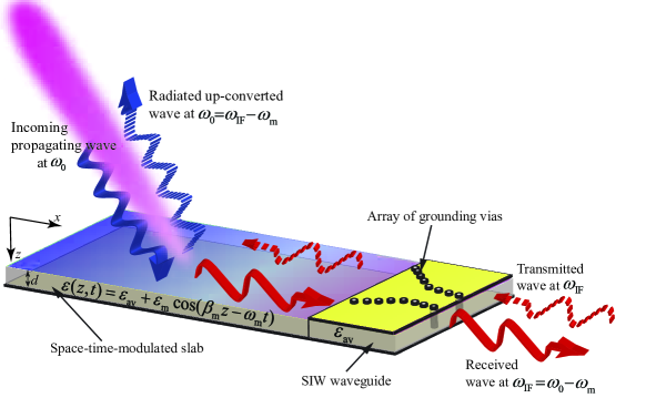
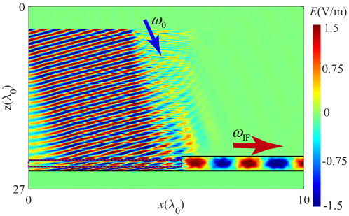
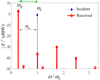
Figure 6: FDTD simulation results of the antenna-mixer-amplifier space-time surface wave medium with $\omega_{0}/\omega_{\text{m}}=1.363$, $\epsilon_{\text{m}}=0.45$, $d=0.8\lambda_{0}$, and $\theta_{\text{i}}=15^{\circ}$. (a) Architecture of the medium. (b) Time- and (c) frequency-domain responses for the down-link transition.

Figure 7 shows the time domain FDTD numerical simulation result for the transmission state (up-link). Here, a transition (up-conversion) from the space-time surface wave at $\omega_{\text{IF}}$ to the space-wave at $\omega_{\text{0}}=\omega_{\text{IF}}+\omega_{\text{m}}$ occurs.

Figure 7 plots the frequency domain numerical simulation result for the transmission state (up-link). This plot clearly shows a pure and strong transition (frequency-conversion) from the incident wave to the down-converted space-time surface wave. The 3.52 dB power conversion loss is in agreement with the analytical result in Eq. (25). In addition, the amplitude of the undesired harmonics are more than $27$ dB lower than the amplitude of the down-converted harmonic at $\omega_{\text{0}}$.

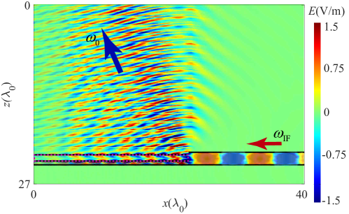
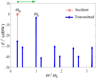
Figure 7: FDTD simulation results of the antenna-mixer-amplifier space-time surface wave medium with $\omega_{0}/\omega_{\text{m}}=1.363$, $\epsilon_{\text{m}}=0.45$, $d=0.8\lambda_{0}$, and $\theta_{\text{i}}==15^{\circ}$. (a) and (b) Time-domain and frequency-domain responses for the up-link transition.

VI Conclusions

We showed that a space-time-varying medium operates as an antenna-mixer-amplifier. Such a unique functionality is achieved by taking advantages of space-time surface waves associated with complex space-time wave vectors in a subluminal space-time medium. The proposed structure is endowed with pure frequency up- and down-conversions and very weak undesired time harmonics. In contrast to the recently proposed space-time mixers, a large frequency ratio between the incident wave frequency and the up-/down-converted wave frequency, with a down- or up-conversion gain, is achievable. Furthermore, as the structure does not operate based on progressive energy transition between the space-time modulation and the incident wave, it possesses a subwavelength thickness (metasurface). Such a multi-functional, highly efficient and compact medium represents a new class of integrated electronic-electromagnetic component, and is expected to find various applications in modern wireless telecommunication systems.

SUPPLEMENTAL MATERIAL

The antenna-mixer-amplifier space-time medium is placed between $z=0$ and $z=d$, and represented by the space-time-varying permittivity of

$$\epsilon_{\text{eq}}(z,t)=\epsilon_{\text{av}}+\epsilon_{\text{m}}\cos(\beta_{\text{m}}z-\omega_{\text{m}}t),$$ (S1)

and $\mu=\mu_{0}$. The electric field inside the slab is defined based on the superposition of the $m=0$ and $m=-1$ space-time harmonics fields, i.e.,

$$E_{\text{S}}(x,z,t)=E_{0}(z)e^{-i\left(k_{x}x+\gamma_{z,0}z-\omega_{0}t\right)}+E_{-1}(z)e^{-i\left(k_{x}x+\gamma_{z,-1}z-\omega_{-1}t\right)},$$ (S2)

where $\omega_{-1}=\omega_{0}-\omega_{\text{m}}$. The corresponding homogeneous wave equation reads

$$\frac{\partial^{2}\textbf{E}}{\partial x^{2}}+\frac{\partial^{2}\textbf{E}}{\partial z^{2}}=\frac{1}{c^{2}}\frac{\partial^{2}[\epsilon_{\text{eq}}(t,z)\textbf{E}]}{\partial t^{2}}.$$ (S3)

Inserting the electric field in (S2) into the wave equation in (S3) results in

$$\begin{split}&\left(\frac{\partial^{2}}{\partial x^{2}}+\frac{\partial^{2}}{\partial z^{2}}\right)\left[E_{0}(z)e^{-i\left(k_{x}x+\gamma_{z,0}z-\omega_{0}t\right)}+E_{-1}(z)e^{-i\left(k_{x}x+\gamma_{z,-1}z-\omega_{-1}t\right)}\right]\\ &\qquad=\frac{1}{c^{2}}\frac{\partial^{2}}{\partial t^{2}}\left(\bigg{[}\epsilon_{\text{av}}+\frac{\epsilon_{\text{m}}}{2}e^{i(\beta_{\text{m}}z-\omega_{\text{m}}t)}+\frac{\epsilon_{\text{m}}}{2}e^{-i(\beta_{\text{m}}z-\omega_{\text{m}}t)}\right]\\ &\qquad\qquad\times\left(E_{0}(z)e^{-i\left(k_{x}x+\gamma_{z,0}z-\omega_{0}t\right)}+E_{-1}(z)e^{-i\left(k_{x}x+\gamma_{z,-1}z-\omega_{-1}t\right)}\right)\bigg{)},\end{split}$$ (S4)

and applying the space and time derivatives, while using a slowly varying envelope approximation (i.e., $\partial^{2}E_{-1}(z)/\partial z^{2}=0$ and $\partial^{2}E_{0}(z)/\partial z^{2}=0$), yields

$$\begin{split}&\left[(k_{x}^{2}+\gamma_{z,0}^{2})E_{0}(z)-2i\gamma_{z,0}\frac{\partial E_{0}(z)}{\partial z}\right]e^{-i\left(k_{x}x+\gamma_{z,0}z-\omega_{0}t\right)}\\ &\qquad+\left[(k_{x}^{2}+\gamma_{z,-1}^{2})E_{-1}(z)-2i\gamma_{z,-1}\frac{\partial E_{-1}(z)}{\partial z}\right]e^{-i\left(k_{x}x+\gamma_{z,-1}z-\omega_{-1}t\right)}\\ &\qquad\qquad=\frac{1}{c^{2}}\left(\bigg{[}\omega_{0}^{2}\epsilon_{\text{av}}+\frac{\epsilon_{\text{m}}}{2}(\omega_{0}-\omega_{\text{m}})^{2}e^{i(\beta_{\text{m}}z-\omega_{\text{m}}t)}+\frac{\epsilon_{\text{m}}}{2}(\omega_{0}+\omega_{\text{m}})^{2}e^{-i(\beta_{\text{m}}z-\omega_{\text{m}}t)}\right]E_{0}(z)e^{-i\left(k_{x}x+\gamma_{z,0}z-\omega_{0}t\right)}\\ &\qquad\qquad+\left[\omega_{-1}^{2}\epsilon_{\text{av}}+\frac{\epsilon_{\text{m}}}{2}(\omega_{0}-2\omega_{\text{m}})^{2}e^{i(\beta_{\text{m}}z-\omega_{\text{m}}t)}+\frac{\epsilon_{\text{m}}}{2}\omega_{0}^{2}e^{-i(\beta_{\text{m}}z-\omega_{\text{m}}t)}\right]E_{-1}(z)e^{-i\left(k_{x}x+\gamma_{z,-1}z-\omega_{-1}t\right)}\bigg{)}.\end{split}$$ (S5)

We then multiply both sides of Eq. (S5) with $e^{i\left(k_{x}x+\gamma_{z,0}z-\omega_{0}t\right)}$, which gives

$$\begin{split}&\left[(k_{x}^{2}+\gamma_{z,0}^{2})E_{0}(z)-2i\gamma_{z,0}\frac{\partial E_{0}(z)}{\partial z}\right]\\ &+\left[(k_{x}^{2}+\gamma_{z,-1}^{2})E_{-1}(z)-2i\gamma_{z,-1}\frac{\partial E_{-1}(z)}{\partial z}\right]e^{i\left(\beta_{\text{m}}-\omega_{\text{m}}t\right)}\\ &\qquad\qquad=\frac{1}{c^{2}}\left(\bigg{[}\omega_{0}^{2}\epsilon_{\text{av}}+\frac{\epsilon_{\text{m}}}{2}(\omega_{0}-\omega_{\text{m}})^{2}e^{i(\beta_{\text{m}}z-\omega_{\text{m}}t)}+\frac{\epsilon_{\text{m}}}{2}(\omega_{0}+\omega_{\text{m}})^{2}e^{-i(\beta_{\text{m}}z-\omega_{\text{m}}t)}\right]E_{0}(z)\\ &\qquad\qquad\qquad+\left[\omega_{-1}^{2}\epsilon_{\text{av}}+\frac{\epsilon_{\text{m}}}{2}(\omega_{0}-2\omega_{\text{m}})^{2}e^{i(\beta_{\text{m}}z-\omega_{\text{m}}t)}+\frac{\epsilon_{\text{m}}}{2}\omega_{0}^{2}e^{-i(\beta_{\text{m}}z-\omega_{\text{m}}t)}\right]E_{-1}(z)e^{i\left(\beta_{\text{m}}-\omega_{\text{m}}t\right)}\bigg{)},\end{split}$$ (S6)

and next, applying $\int_{0}^{\frac{2\pi}{\omega_{\text{m}}}}dt$ to both sides of (S6) yields

$$\frac{dE_{0}(z)}{dz}=i\dfrac{\epsilon_{\text{m}}k_{0}^{2}}{4\gamma_{z,0}}E_{-1}(z).$$ (S7)

Following the same procedure, we next multiply both sides of (S6) with $e^{-i\left(\beta_{\text{m}}z-\omega_{\text{m}}t\right)}$, and applying $\int_{0}^{\frac{2\pi}{\omega_{\text{m}}}}dt$ in both sides of the resultant, which reduces to

$$\left[(k_{x}^{2}+\gamma_{z,-1}^{2})E_{-1}(z)-2i\gamma_{z,-1}\frac{dE_{-1}(z)}{dz}\right]=\frac{\omega_{-1}^{2}}{c^{2}}\left(\frac{\epsilon_{\text{m}}}{2}E_{0}(z)+\epsilon_{\text{av}}E_{-1}(z)\right),$$ (S8)

$$\frac{dE_{-1}(z)}{dz}=i\dfrac{\epsilon_{\text{m}}k_{-1}^{2}}{4\gamma_{z,-1}}E_{0}(z),$$ (S9)

where $k_{-1}=\omega_{-1}/c^{2}$. Solving the coupled equations (S7) and (S9) together, we achieve the field coefficients $E_{0}(z)$ and $E_{-1}(z)$ as given in Eqs.(17) and (18) for the reception state and in Eqs.(23) and (24) for the transmission state.

References

- (1) G. Vannucci, “Wireless telecommunication system,” 1995, US Patent 5,459,727.
- (2) S. R. Saunders and A. Aragón-Zavala, Antennas and propagation for wireless communication systems. John Wiley & Sons, 2007.
- (3) S. Taravati and C. Caloz, “Mixer-duplexer-antenna leaky-wave system based on periodic space-time modulation,” IEEE Trans. Antennas Propagat., vol. 65, no. 2, pp. 442 – 452, Feb. 2017.
- (4) S. Taravati and A. A. Kishk, “Dynamic modulation yields one-way beam splitting,” Phys. Rev. B, vol. 99, no. 7, p. 075101, Jan. 2019.
- (5) A. Alvarez-Melcon, X. Wu, J. Zang, X. Liu, and J. S. Gomez-Diaz, “Coupling matrix representation of nonreciprocal filters based on time-modulated resonators,” IEEE Trans. Microw. Theory Techn., vol. 67, no. 12, pp. 4751–4763, 2019.
- (6) X. Wu, X. Liu, M. D. Hickle, D. Peroulis, J. S. Gómez-Díaz, and A. Á. Melcón, “Isolating bandpass filters using time-modulated resonators,” IEEE Trans. Microw. Theory Techn., vol. 67, no. 6, pp. 2331–2345, 2019.
- (7) S. Taravati and G. V. Eleftheriades, “Generalized space-time periodic diffraction gratings: Theory and applications,” Phys. Rev. Appl., vol. 12, no. 2, p. 024026, 2019.
- (8) Y. Shi and S. Fan, “Dynamic non-reciprocal meta-surfaces with arbitrary phase reconfigurability based on photonic transition in meta-atoms,” Appl. Phys. Lett., vol. 108, p. 021110, Jan. 2016.
- (9) Y. Shi, S. Han, and S. Fan, “Optical circulation and isolation based on indirect photonic transitions of guided resonance modes,” ACS Photonics, vol. 4, no. 7, pp. 1639–1645, Jun. 2017.
- (10) M. M. Salary, S. Jafar-Zanjani, and H. Mosallaei, “Electrically tunable harmonics in time-modulated metasurfaces for wavefront engineering,” New J. Phys., vol. 20, no. 12, p. 123023, 2018.
- (11) M. M. Salary, S. Farazi, and H. Mosallaei, “A dynamically modulated all-dielectric metasurface doublet for directional harmonic generation and manipulation in transmission,” Adv. Opt. Mater., p. 1900843, 2019.
- (12) S. Taravati and A. A. Kishk, “Advanced wave engineering via obliquely illuminated space-time-modulated slab,” IEEE Trans. Antennas Propagat., vol. 67, no. 1, pp. 270–281, 2019.
- (13) J. W. Zang, D. Correas-Serrano, J. T. S. Do, X. Liu, A. Alvarez-Melcon, and J. S. Gomez-Diaz, “Nonreciprocal wavefront engineering with time-modulated gradient metasurfaces,” Phys. Rev. Appl., vol. 11, no. 5, p. 054054, 2019.
- (14) S. Inampudi, M. M. Salary, S. Jafar-Zanjani, and H. Mosallaei, “Rigorous space-time coupled-wave analysis for patterned surfaces with temporal permittivity modulation,” Opt. Mater. Express, vol. 9, no. 1, pp. 162–182, 2019.
- (15) S. Y. Elnaggar and G. N. Milford, “Generalized space-time periodic circuits for arbitrary structures,” arXiv preprint arXiv:1901.08698, 2019.
- (16) N. Wang, Z.-Q. Zhang, and C. Chan, “Photonic floquet media with a complex time-periodic permittivity,” Phys. Rev. B, vol. 98, no. 8, p. 085142, 2018.
- (17) Z. Wu and A. Grbic, “Serrodyne frequency translation using time-modulated metasurfaces,” IEEE Trans. Antennas Propagat., 2019.
- (18) S. Taravati and A. A. Kishk, “Space-time modulation: Principles and applications,” IEEE Microw. Mag., vol. 21, no. 4, pp. 30–56, 2020.
- (19) G. A. Ptitcyn, M. S. Mirmoosa, and S. A. Tretyakov, “Time-modulated meta-atoms,” Phys. Rev. Res., vol. 1, no. 2, p. 023014, 2019.
- (20) H. B. Sedeh, M. M. Salary, and H. Mosallaei, “Topological space-time photonic transitions in angular-momentum-biased metasurfaces,” Advanced Optical Materials.
- (21) Z.-X. Du, A. Li, X. Y. Zhang, and D. F. Sievenpiper, “A simulation technique for radiation properties of time-varying media based on frequency-domain solvers,” IEEE Access, vol. 7, pp. 112 375–112 383, 2019.
- (22) X. Wang, A. Diaz-Rubio, H. Li, S. A. Tretyakov, and A. Alu, “Theory and design of multifunctional space-time metasurfaces,” Phys. Rev. Appl., vol. 13, no. 4, p. 044040, 2020.
- (23) S. Taravati and G. V. Eleftheriades, “Full-duplex nonreciprocal-beam-steering metasurfaces comprising time-modulated twin meta-atoms,” arXiv preprint arXiv:1911.04033, 2019.
- (24) A. Li, Y. Li, J. Long, E. Forati, Z. Du, and D. Sievenpiper, “Time-moduated nonreciprocal metasurface absorber for surface waves,” Optics Letters, vol. 45, no. 5, pp. 1212–1215, 2020.
- (25) H. B. Sedeh, M. M. Salary, and H. Mosallaei, “Topological space-time photonic transitions in angular-momentum-biased metasurfaces,” Adv. Opt. Mater., 2020.
- (26) S. Taravati, “Application of space-and time-modulated dispersion engineered metamaterials to signal processing and magnetless nonreciprocity,” Ph.D. dissertation, École Polytechnique de Montréal, 2017.
- (27) J. L. Wentz, “A nonreciprocal electrooptic device,” Proc. IEEE, vol. 54, no. 1, pp. 97–98, 1966.
- (28) S. Taravati, N. Chamanara, and C. Caloz, “Nonreciprocal electromagnetic scattering from a periodically space-time modulated slab and application to a quasisonic isolator,” Phys. Rev. B, vol. 96, no. 16, p. 165144, Oct. 2017.
- (29) S. Taravati, “Self-biased broadband magnet-free linear isolator based on one-way space-time coherency,” Phys. Rev. B, vol. 96, no. 23, p. 235150, Dec. 2017.
- (30) ——, “Giant linear nonreciprocity, zero reflection, and zero band gap in equilibrated space-time-varying media,” Phys. Rev. Appl., vol. 9, no. 6, p. 064012, Jun. 2018.
- (31) M. Oudich, Y. Deng, M. Tao, and Y. Jing, “Space-time phononic crystals with anomalous topological edge states,” Phys. Rev. Res., vol. 1, no. 3, p. 033069, 2019.
- (32) M. Chegnizadeh, M. Memarian, and K. Mehrany, “Non-reciprocity using quadrature-phase time-varying slab resonators,” J. Opt. Soc. Am. B, vol. 37, no. 1, pp. 88–97, 2020.
- (33) S. Taravati, “Aperiodic space-time modulation for pure frequency mixing,” Phys. Rev. B, vol. 97, no. 11, p. 115131, 2018.
- (34) H. Shanks, “A new technique for electronic scanning,” IEEE Trans. Antennas Propag., vol. 9, no. 2, pp. 162–166, 1961.
- (35) Y. Hadad, J. C. Soric, and A. Alù, “Breaking temporal symmetries for emission and absorption,” Proc. Natl. Acad. Sci., vol. 113, no. 13, pp. 3471–3475, 2016.
- (36) D. Ramaccia, D. L. Sounas, A. Alù, F. Bilotti, and A. Toscano, “Nonreciprocity in antenna radiation induced by space-time varying metamaterial cloaks,” IEEE Antennas Wirel. Propagat. Lett., vol. 17, no. 11, pp. 1968–1972, 2018.
- (37) S. Taravati and A. A. Kishk, “Space-time-varying surface-wave antenna,” in 2018 18th International Symposium on Antenna Technology and Applied Electromagnetics (ANTEM). IEEE, 2018.
- (38) M. M. Salary, S. Jafar-Zanjani, and H. Mosallaei, “Nonreciprocal optical links based on time-modulated nanoantenna arrays: Full-duplex communication,” Phys. Rev. B, vol. 99, no. 4, p. 045416, 2019.
- (39) J. Zang, X. Wang, A. Alvarez-Melcon, and J. S. Gomez-Diaz, “Nonreciprocal yagi–uda filtering antennas,” IEEE Antennas Wirel. Propagat. Lett., vol. 18, no. 12, pp. 2661–2665, 2019.
- (40) J. Li, C. Shen, X. Zhu, Y. Xie, and S. A. Cummer, “Nonreciprocal sound propagation in space-time modulated media,” Phys. Rev. B, vol. 99, no. 14, p. 144311, 2019.
- (41) D. C. Serrano, A. Alù, and J. S. Gomez-Diaz, “Magnetic-free nonreciprocal photonic platform based on time-modulated graphene capacitors,” Phys. Rev. B, vol. 98, no. 16, p. 165428, 2018.
- (42) M. Liu, D. A. Powell, Y. Zarate, and I. V. Shadrivov, “Huygens’ metadevices for parametric waves,” vol. 8, no. 3, p. 031077, 2018.
- (43) S. Y. Elnaggar and G. N. Milford, “Modelling space-time periodic structures with arbitrary unit cells using time periodic circuit theory,” arXiv preprint arXiv:1901.08698, 2019.
- (44) S. Taravati and G. V. Eleftheriades, “Mixer-antenna medium,” in 2019 13th International Congress on Artificial Materials for Novel Wave Phenomena (Metamaterials). IEEE, 2019.
- (45) S. Taravati and C. Caloz, “Space-time modulated nonreciprocal mixing, amplifying and scanning leaky-wave antenna system,” in IEEE AP-S Int. Antennas Propagat. (APS), Vancouver, Canada, 2015.
- (46) Z. Yu and S. Fan, “Complete optical isolation created by indirect interband photonic transitions,” Nat. Photonics, vol. 3, pp. 91 – 94, Jan. 2009.
- (47) H. Lira, Z. Yu, S. Fan, and M. Lipson, “Electrically driven nonreciprocity induced by interband photonic transition on a silicon chip,” Phys. Rev. Lett., vol. 109, p. 033901, Jul. 2012.
- (48) N. Chamanara, S. Taravati, Z.-L. Deck-Léger, and C. Caloz, “Optical isolation based on space-time engineered asymmetric photonic bandgaps,” Phys. Rev. B, vol. 96, no. 15, p. 155409, Oct. 2017.
- (49) A. L. Cullen, “A travelling-wave parametric amplifier,” Nature, vol. 181, p. 332, Feb. 1958.
- (50) P. Tien and H. Suhl, “A traveling-wave ferromagnetic amplifier,” Proc. IEEE, vol. 46, no. 4, pp. 700–706, 1958.