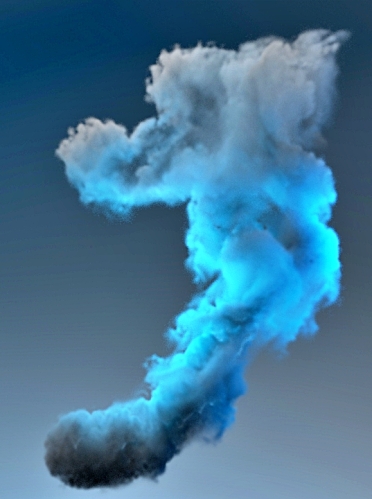
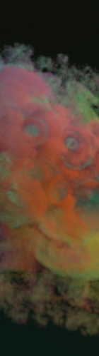
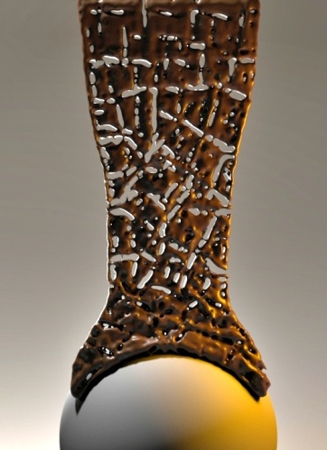
Figure 1. Our Lagrangian neural style transfer enables novel artistic manipulations, such as time-coherent stylization of smoke, multiple fluids and liquids.

Lagrangian Neural Style Transfer for Fluids

Abstract.

Artistically controlling the shape, motion and appearance of fluid simulations pose major challenges in visual effects production. In this paper, we present a neural style transfer approach from images to 3D fluids formulated in a Lagrangian viewpoint. Using particles for style transfer has unique benefits compared to grid-based techniques. Attributes are stored on the particles and hence are trivially transported by the particle motion. This intrinsically ensures temporal consistency of the optimized stylized structure and notably improves the resulting quality. Simultaneously, the expensive, recursive alignment of stylization velocity fields of grid approaches is unnecessary, reducing the computation time to less than an hour and rendering neural flow stylization practical in production settings. Moreover, the Lagrangian representation improves artistic control as it allows for multi-fluid stylization and consistent color transfer from images, and the generality of the method enables stylization of smoke and liquids likewise.

1. Introduction

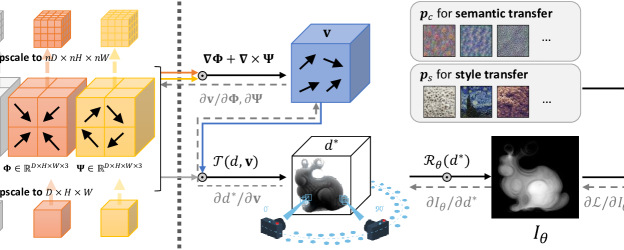
Figure 2. Overview of our LNST method. We optimize particle positions $\mathbf{x}^{\circ}$ and attributes $\lambda^{\circ}$ to stylize a given density field $d^{*}$. We transfer information from particles to the grid with the splatting operation $\mathcal{I}_{p2g}$, and jointly update loss functions and attributes. The black arrows show the direction of the feed-forward pass to the loss network $L$, and the gray arrows indicate backpropagation for computing gradients. For grid-based simulation inputs, we sample and re-simulate particles in a multi-scale manner (Algorithm (1)).

In visual effects production, physics-based simulations are not only used to realistically re-create natural phenomena, but also as a tool to convey stories and trigger emotions. Hence, artistically controlling the shape, motion and the appearance of simulations is essential for providing directability for physics. Specifically to fluids, the major challenge is the non-linearity of the underlying fluid motion equations, which makes optimizations towards a desired target difficult. Keyframe matching either through expensive fully-optimized simulations [Treuille et al., 2003; McNamara et al., 2004; Pan and Manocha, 2017] or simpler distance-based forces [Nielsen and Bridson, 2011; Raveendran et al., 2012] provide control over the shape of fluids. The fluid motion can be enhanced with turbulence synthesis approaches [Kim et al., 2008; Sato et al., 2018] or guided by coarse grid simulations [Nielsen and Bridson, 2011], while patch-based texture composition [Gagnon et al., 2019; Jamriška et al., 2015] enables manipulation over appearance by automatic transfer of input 2D image patterns.

The recently introduced Transport-based Neural Style Transfer (TNST) [Kim et al., 2019a] takes flow appearance and motion control to a new level: arbitrary styles and semantic structures given by 2D input images are automatically transferred to 3D smoke simulations. The achieved effects range from natural turbulent structures to complex artistic patterns and intricate motifs. The method extends traditional image-based Neural Style Transfer [Gatys et al., 2016] by reformulating it as a transport-based optimization. Thus, TNST is physically inspired, as it computes the density transport from a source input smoke to a desired target configuration, allowing control over the amount of dissipated smoke during the stylization process. However, TNST faces challenges when dealing with time coherency due to its grid-based discretization. The velocity field computed for the stylization is performed independently for each time step, and the individually computed velocities are recursively aligned for a given window size. Large window sizes are required, rendering the recursive computation expensive while still accumulating inaccuracies in the alignment that can manifest as discontinuities. Moreover, transport-based style transfer is only able to advect density values that are present in the original simulation, and therefore it does not inherently support color information or stylizations that undergo heavy structural changes.

Thus, in this work, we reformulate Neural Style Transfer in a Lagrangian setting (see Figure 2), demonstrating its superior properties compared to its Eulerian counterpart. In our Lagrangian formulation, we optimize per-particle attributes such as positions, densities and color. This intrinsically ensures better temporal consistency as shown for example in Figure 3, eliminating the need for the expensive recursive alignment of stylization velocity fields. The Lagrangian approach reduces the computational cost to enforce time coherency, increasing the speed of results from one day to a single hour. The Lagrangian Style transfer framework is completely oblivious to the underlying fluid solver type. Since the loss function is based on filter activations from pre-trained classification networks, we transfer the information back and forth from particles to the grids, where loss functions and attributes can be jointly updated. We propose regularization strategies that help to conserve the mass of the underlying simulations, avoiding oversampling of stylization particles. Our results demonstrate novel artistic manipulations, such as stylization of liquids, color stylization, stylization of multiple fluids, and time-varying stylization.

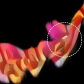
Figure 3. Neural color stylization [Christen et al., 2019] using the input Red Canna applied to a smoke scene with TNST (top) and LNST (bottom). The close-up views (dashed box, frames 60 and 66) reveal that LNST is more time-coherent than TNST (dashed circle).

2. Related Work

Lagrangian Fluids have become popular for simulating incompressible fluids and interactions with various materials. Since the introduction of SPH to computer graphics [Desbrun and Gascuel, 1996; Müller et al., 2003], various extensions have been presented that made it possible to efficiently simulate millions of particles on a single desktop computer. Accordingly, particle methods reached an unprecedented level of visual quality, where fine-scale surface effects and flow details are reliably captured. To enforce incompressibility, the original state equation based method [Monaghan, 2005; Becker and Teschner, 2007] has been replaced by pressure Poisson equation (PPE) solvers using either a single source term for density invariance [Solenthaler and Pajarola, 2009; Ihmsen et al., 2014] or two PPEs to additionally account for divergence-free velocities [Bender and Koschier, 2015]. Solvers closely related to PPE have been presented, such as Local Poisson SPH [He et al., 2012], Constraint Fluids [Servin et al., 2012] and Position-based Fluids [Macklin and Mueller, 2013]. Boundary handling is computed with particle-based approaches that sample boundary geometry (e.g. [Gissler et al., 2019]) or implicit methods that typically use a signed distance field (e.g. [Koschier and Bender, 2017]). Extensions include highly viscous fluids (e.g. [Peer et al., 2015]), and multiple phases and fluid mixing (e.g. [Ren et al., 2014]). An overview of recent developments in SPH can be found in the course notes of Koschier et al. [2019].

Hybrid Lagrangian-Eulerian Fluids combine the versatility of the particles representation to track transported quantities with the capacity of grids to enforce incompressibility. Among popular approaches, the Fluid Implicit Particle Method (FLIP) [Brackbill et al., 1988] was first employed in graphics to animate sand and water [Zhu and Bridson, 2005]. Due to its ability to accurately capture sub-grid details it has been widely adopted for liquid simulations, being extended to animation of turbulent water [Kim et al., 2006], coupled with SPH for modelling small scale splashes [Losasso et al., 2008], improved for efficiency [Ando et al., 2013; Ferstl et al., 2016], used in fluid control [Pan et al., 2013], and enhanced with better particle distribution [Ando and Tsuruno, 2011; Um et al., 2014]. The Material Point Method (MPM) [Stomakhin et al., 2013] was used to simulate a wide class of solid materials [Jiang et al., 2016]. Recent work on hybrid approaches extended the information tracked by the particles by affine [Jiang et al., 2015] and polynomial [Fu et al., 2017] transformations. For a thorough discussion of hybrid continuum models, we refer to Hu et al. [2019b].

Patch-based Appearance Transfer methods compute similarities between source and target datasets in local neighborhoods, modifying the appearance of the source by transferring best-matched features from the target dataset. Kwatra et al. [2005] employ local similarity measures in an energy-based optimization, enabling texture patches animated by flow fields. This approach was further extended to liquid surfaces [Kwatra et al., 2006; Bargteil et al., 2006], and improved by modifying the texture based on visually salient features of the liquid mesh [Narain et al., 2007]. Jamriška et al. [2015] improved previous work with better temporal coherency and matching precision for obtaining high-quality 2D textured fluids. Texturing liquid simulations was also implemented in a Lagrangian framework by using individually tracked surface patches [Yu et al., 2011; Gagnon et al., 2016; Gagnon et al., 2019]. Image and video-based approaches also take inspiration from fluid transport. Bousseau et al. [2007] proposed a bidirectional advection scheme to reduce patch distortions. Regenerative morphing and image melding techniques were combined with patch-based tracking to produce in-betweens for artist-stylized keyframes [Browning et al., 2014]. Recent advances in patch-based appearance transfer often rely on evaluating the underlying 3D geometric information; examples include improving template matching by a novel similarity measure [Talmi et al., 2017], patch matching for illumination effects [Fišer et al., 2016], extensions to texture mapping [Bi et al., 2017] and intricate texture motifs [Diamanti et al., 2015]. While these approaches were successful in 2D settings and for texturing liquids, they cannot inherently support 3D volumetric data.

Velocity Synthesis methods augment flow simulations with velocity fields, which manipulate or enhance volumetric data. Due to the inability of pressure-velocity formulations to properly conserve different energy scales of flow phenomena, sub-grid turbulence [Kim et al., 2008; Schechter and Bridson, 2008; Narain et al., 2008] was modelled for better energy conservation. These approaches were extended to model turbulence in the wake of solid boundaries [Pfaff et al., 2009], liquid surfaces [Kim et al., 2013] and example-based turbulence synthesis [Sato et al., 2018]. In order to merge fluids of different simulation instances [Thuerey, 2016] or separated by void regions [Sato et al., 2018], velocity fields where synthesized by solving an unconstrained energy minimization problem. Lastly, the Transport-based Neural Style Transfer (TNST) [Kim et al., 2019a] can also be seen as a velocity synthesis method: at each time-step, the method optimizes a velocity field that transports the smoke towards a desired stylization.

Machine Learning & Fluids was first introduced to graphics by Ladický et al. [2015]. They used Regression Forests to predict positions of fluid particles over time, resulting in a substantial performance gain compared to traditional Lagrangian solvers. CNN-based architectures were employed in Eulerian-based solvers to substitute the pressure projection step [Tompson et al., 2017; Yang et al., 2016] and to synthesize flow simulations from a set of reduced parameters [Kim et al., 2019b]. An LSTM architecture [Wiewel et al., 2019] predicted changes on pressure fields for multiple subsequent time-steps, speeding up the pressure projection step. Differentiable fluid solvers [Schenck and Fox, 2018; Hu et al., 2019a, 2020; Holl et al., 2020] have been introduced that can be automatically coupled with deep learning architectures and provide a natural interface for image-based applications. Patch-based [Chu and Thuerey, 2017] and GAN-based [Xie et al., 2018] fluid super-resolution enhance coarse simulations with rich turbulence details, while also being computationally inexpensive. While these approaches produce detailed, high-quality results, they do not support transfer of arbitrary smoke styles.

Differentiable Rendering and Stylization is used in Neural Style Transfer algorithms to transfer the style of a source image to a target image by matching features of a pre-trained classified network [Gatys et al., 2016]. However, stylizing 3D data requires a differentiable renderer to map the representation to image space. Loper and Black [2014] proposed the first fully differentiable renderer with automatically computed derivatives, while a novel differentiable volume sampling was implemented by Yan et al. [2016]. Raster-based differentiable rendering for meshes for stylization with approximate [Kato et al., 2018] and analytic [Liu et al., 2018] derivatives was proposed to approximate visibility changes and mesh filters, respectively. A cubic stylization algorithm [Liu and Jacobson, 2019] was implemented by minimizing a constrained energy formulation and employed to mesh stylization. Closer to our work, Kim et al. [2019a] defines an Eulerian framework for a transport-based neural style transfer of smoke. Their approach computes individually stylized velocity fields per-frame, and temporal coherence is enforced by aligning subsequent stylization velocity fields and performing smoothing. We compare the Eulerian approach with our method in the subsequent sections. For an overview on differentiable rendering and neural style transfer we refer to Yifan et al. [2019] and Jing et al. [2019], respectively.

3. Eulerian Transport-Based NST

We briefly review previous Eulerian-based TNST [Kim et al., 2019a] for completeness and to better compare against our novel Lagrangian approach. Transport-Based Neural Style Transfer (TNST) extends the original NST algorithm to transfer the style of a given image to a flow-based 3D smoke density. As opposed to NST where individual pixels of the target image are optimized, TNST optimizes a velocity field that modifies density values through indirect smoke transport. The velocity field $\hat{\mathbf{v}}$ that stylizes the input density $d$ is defined by a loss function $\mathcal{L}$ computed from a pre-trained image classification CNN by

(1) $$\hat{\mathbf{v}}=\operatorname*{arg\,min}_{\mathbf{v}}\sum_{\theta\in\Theta}\mathcal{L}(\mathcal{R}_{\theta}(\mathcal{T}(d,\mathbf{v}))\,,\mathbf{p}),$$

where $\mathcal{T}$ is a transport function that advects $d$ with $\mathbf{v}$, generating the stylized density $\hat{d}=\mathcal{T}(d,\hat{\mathbf{v}})$; $\mathcal{R}$ is a differentiable renderer converting the density field to image-space for a specific view $\theta$ by $I=\mathcal{R}_{\theta}(\hat{d})$, and $\mathbf{p}$ denotes the set of user-defined parameters used in the stylization process. The velocity field contributions are individually computed per view, resulting in a 3D volumetric smoke stylization. While the authors separate the velocity field into its irrotational and incompressible parts which can be optimized independently, we omit this here for simplicity.

The loss function is subdivided into semantic and style losses for additional control over artistic stylization given a rendered density field. Style transfer considers an input image and user-selected activation layers (levels of features), while semantic transfer selects a CNN layer with desirable attributes that will be transferred to the target stylized smoke. Since the smoke is advected towards a target objective, this guarantees that the original smoke shape and semantics is enforced without matching its original content loss, as in traditional NST algorithms [Gatys et al., 2015]. For simplicity, we restrict our discussion to the style loss, which is given by

(2) $$\mathcal{L}_{s}(I,\mathbf{p}_{s})=\sum_{l}^{L}\left[\frac{1}{4C_{l}^{2}(H_{l}\times W_{l})^{2}}\sum_{m,n}^{C_{l}}\left(G^{l}_{mn}(I)-G^{l}_{mn}(I_{s})\right)^{2}\right],$$

where the Gram matrix $G$ computes correlations between different filter responses. The Gram matrix is calculated for a given layer $l$ and two channels $m$ and $n$, by iterating over all pixels of the flattened 1-D feature map $\mathcal{\hat{F}}^{l}(I)$ as

(3) $$G^{l}_{mn}(I)=\sum_{i}^{H_{l}\times W_{l}}\mathcal{\hat{F}}_{mi}^{l}(I)\;\mathcal{\hat{F}}_{ni}^{l}(I).$$

Extending the single frame stylization in a time-coherent fashion is expensive and inaccurate when computed in an Eulerian framework. TNST aligns stylization velocities by recursively advecting them with the simulation velocities for a given window size as shown in Figure 4. The recursive nature renders this computation inefficient time- and memory-wise, especially when large window sizes are employed to enable smooth transitions between consecutive frames. Due to the large memory requirement, this operation often has to be computed on the CPU, which generates additional overhead by the use of expensive data transfer operations.

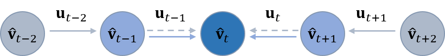
Figure 4. Recursive temporal alignment in TNST. For a window size $w$, $(w^{2}-1)/4$ recursive temporal alignment steps are performed for each stylization velocity $\hat{\mathbf{v}}$. Colors indicate the distance to frame $t$, and arrows refer to advection steps (with recursive steps shown as dashed lines).

4. Lagrangian NST

In contrast to its Eulerian counterpart, the Lagrangian representation uses particles that carry quantities such as the position, density and color value. Neural style transfer methods compute loss functions based on filter activations from pre-trained classification networks, which are trained on image datasets. Thus, we have to transfer the information back and forth from particles to the grids, where loss functions and attributes can be jointly updated. We take inspiration from hybrid Lagrangian-Eulerian fluid simulation pipelines that use grid-to-particle $\mathcal{I}_{g2p}$ and particle-to-grid $\mathcal{I}_{p2g}$ transfers as

(4) $$\lambda^{\circ}=\mathcal{I}_{g2p}(\mathbf{x}^{\circ},\lambda^{\framebox{\small{+}}})\;\;\;\text{and}\;\;\;\lambda^{\framebox{\small{+}}}=\mathcal{I}_{p2g}(\mathbf{x}^{\circ},\lambda^{\circ},h,\mathbf{x}^{\framebox{\small{+}}}),$$

where $\lambda^{\circ}$ and $\lambda^{\framebox{\small{+}}}$ are attributes defined on the particle and grid, respectively, $\mathbf{x}^{\circ}$ refers to all particle positions, $\mathbf{x}^{\framebox{\small{+}}}$ are grid nodes to which values are transferred, and $h$ is the support size of the particle-to-grid transfer.

Our grid-to-particle transfer employs a regular grid cubic interpolant, while the particle-to-grid transfer uses standard radial basis functions. Regular Cartesian grids facilitate finding grid vertices around an arbitrary particle position. For this, we extended a differentiable point cloud projector [Insafutdinov and Dosovitskiy, 2018] to arbitrary grid resolution, neighborhood size and custom kernel functions. Given all the neighboring particles $j\in\partial\Omega_{\mathbf{x}}$ around a grid node $\mathbf{x}$, a grid attribute $\lambda^{\framebox{\small{+}}}$ is computed by summing up weighted particle contributions as

(5) $$\lambda^{\framebox{\small{+}}}(\mathbf{x})=\frac{\sum_{j\in\partial\Omega_{\mathbf{x}}}\lambda_{j}^{\circ}\;W(||\mathbf{x}-\mathbf{x_{j}}^{\circ}||,h)}{\sum_{j\in\partial\Omega_{\mathbf{x}}}W(||\mathbf{x}-\mathbf{x_{j}}^{\circ}||,h)},$$

where we chose $W$ to be the cubic B-spline kernel, which is also often used in SPH simulations [Monaghan, 2005]:

(6) $$W(r,h)_{\text{cubic}}=\begin{cases}\frac{2}{3}-r^{2}+\frac{1}{2}r^{3},&0\leq r\leq 1,\\ \frac{1}{6}(2-r)^{3},&1\leq r\leq 2,\\ 0,&r>2.\end{cases}$$

We now have all the necessary elements to convert the previous Eulerian style transfer (Equation (1)) into a Lagrangian framework. Given a set of Lagrangian attributes $\mathbf{\Lambda}^{\circ}$, the optimization objective for a single frame is

(7) $$\hat{\mathbf{\Lambda}}^{\circ}=\operatorname*{arg\,min}_{\mathbf{\Lambda}^{\circ}}\>\sum_{\theta\in\Theta}\sum_{\lambda^{\circ}\in\Lambda^{\circ}}w_{\lambda^{\circ}}\,\mathcal{L}(\mathcal{R}_{\theta}(\mathcal{I}_{p2g}(\mathbf{x}^{\circ},\lambda^{\circ}),\,\mathbf{p}),$$

where $w_{\lambda^{\circ}}$ are weights for the losses that include Lagrangian attributes. In case of particle position $\mathbf{x}^{\circ}$ given as the target quantity $\lambda^{\circ}$, we use the SPH density $\mathcal{I}_{p2g}(\mathbf{x}^{\circ})=\sum_{j\in\partial\Omega_{\mathbf{x}}}{m_{j}W(||\mathbf{x}-\mathbf{x}_{j}^{\circ}||,h)}$, where $m_{j}$ represents the mass of the $j$-th particle [Bender, 2016]. Note that our losses are evaluated similarly as in the original Eulerian method, since the gradients computed in image-space also modify grid values ($\lambda^{\framebox{\small{+}}}$). However, these gradients are automatically propagated back to the particles by auto-differentiating the particle-to-grid  $\mathcal{I}_{p2g}$ function. Thus, our method only reformulates the domain of the optimization, sharing the same stylization possibilities (semantic and content transfers) as in the original TNST.

Since the Lagrangian optimization is completely oblivious to the underlying solver type, the chosen attributes for creating stylizations can be arbitrarily combined, enabling a wide range of artistic manipulations in different scene setups. We outline two strategies and demonstrate their impact on the stylization. The first one is particularly suitable for participating volumetric data, which are often simulated with grid-based solvers. It involves optimizing a scalar value carried by the Lagrangian stylization particles by Equation (7). For most of our smoke scenes, this scalar value is the density, though it can also be the color or emission. The regularization term

(8) $$\mathcal{L}({\lambda^{\circ}})_{\rho}=(\sum{\Delta\lambda^{\circ}})^{2}-\sum\log{||\Delta\lambda^{\circ}||_{1}}$$

reinforces the conservation of the original amount of smoke. It minimizes the total net smoke change, preventing the stylization to undesirably fade out particles and keeping changes non-zero by minimizing cross-entropy loss at the same time. Figure 5 demonstrates the impact of different regularizer weights.

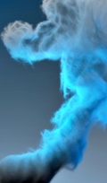
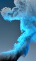
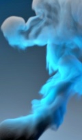
Figure 5. Different weights for the density regularization show the trade-off between pronounced structures and conservation of mass. The images on the left show results with zero, low, and high weights, respectively, and the right image is the ground truth.

The second strategy is suitable if the underlying fluid solver is particle-based or hybrid, which is often the case for liquids. For these simulations, we can define particle position displacements as the optimized Lagrangian attributes. However, generating stylizations by modifying particle displacements may cause cluttering or regions with insufficient particles. The regularization penalizes irregular distribution of particle positions and is defined as

(9) $$\mathcal{L}(\mathbf{x}^{\circ})_{\Delta x}=||\mathcal{I}_{p2g}(\mathbf{x}^{\circ})-\rho_{0}^{\framebox{\small{+}}}||_{2}^{2},$$

where $\rho_{0}^{\framebox{\small{+}}}$ corresponds to the rest density for cells that contain particles, and is zero otherwise. Note that Equation (9) does not account for the particle deficiency near fluid surfaces. This could be addressed by adding virtual particles [Schechter and Bridson, 2008] or applying (variants of) the Shepard correction to the kernel function [Reinhardt et al., 2019]. We show the impact of this regularizer on the particle sampling in Figure 6, highlighting the trade-off between uniform distribution and stylization strength.

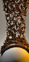
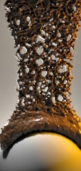
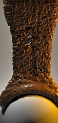
Figure 6. Different weights for the position regularization show the trade-off between pronounced structures and uniform sampling. The images on the left show results with zero, low, and high weights, respectively, and the right image is the ground truth.

We notice that both regularizations in Equation (8) and Equation (9) are different incarnations of the mass conservation property commonly used in fluid simulations. In TNST, mass conservation is enforced by decomposing the stylization velocities into their irrotational and incompressible parts, which can be optimized independently. Both techniques enable a high degree of artistic control over the content manipulation.

4.1. An Efficient Particle-Based Smoke Re-Simulation

If the input is a grid-based simulation, we have to sample and re-simulate particles. We can use a sparse representation with only one particle per voxel, in constrast to hybrid liquid simulations that usually sample 8 particles per voxel to properly capture momentum conservation [Zhu and Bridson, 2005]. Combining a low number of particles with a position integration algorithm that accumulates errors over time will yield irregularly distributed particles [Ando and Tsuruno, 2011]. This manifests in a rendered image as smoke with overly dense or void regions. We therfore solve the following optimization problem

(10) $$\hat{\mathbf{x}}^{\circ},\hat{\rho}^{\circ}=\operatorname*{arg\,min}_{{\mathbf{x}^{\circ},\rho^{\circ}}}\sum_{t}||\mathcal{I}_{p2g}(\mathbf{x}^{\circ}_{t},\rho_{t}^{\circ})-\rho_{t}^{\framebox{\small{+}}}||_{2}^{2}.$$

The optimization problem presented above is not only severely under-constrained but also has a time-varying objective term, and optimizing for Equation (10) is challenging if tackled jointly for both particle positions $\mathbf{x}^{\circ}$ and densities $\rho^{\circ}$. Thus, we use a heuristic approach for solving this optimization, subdividing it into two steps, position optimization and multi-scale density update (Section 4.1.1). Firstly, we minimize the irregular distribution of particle positions by employing a position-based update, optimizing particle distributions using Equation (9) as objective. The distribution of the particles is optimized per frame and serves as an input for optimizing subsequent frames, enabling temporally coherent position updates. Equation (9) can be automatically computed by our fully differentiable pipeline.

4.1.1. Multi-scale Density Representation

In addition to the position update, we also compute smoke densities individually carried by the particles to further eliminate small gaps that may appear due to the sparse discretization, further enhancing the solution of Equation (10). Owing to the low number of sampled particles and the mismatches between grid and particle transfers, carrying a constant density will either produce grainy (Figure 7, (b)) or diffuse (Figure 7, (c)) volumetric representations, depending on if particle re-distribution (Equation (9)) is applied or not. A simple approach is to interpolate density values directly from the grid over time. Larger kernel sizes could be used to remedy sparse sampling, but would excessively smooth structures and degrade quality.

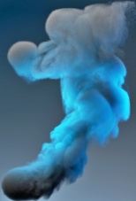
(a) (b) (c)
(d) (e) (f)

Figure 7. Comparison of different re-simulation strategies. (a): ground truth density, (b): constant density carried by particles, (c): (b) with redistribution by Equation (9), (d): single-scale sampled density, (e): (d) with redistribution, (f): multi-scale ($n_{s}=3$) sampled density with redistribution (final method).

We take inspiration from Laplacian pyramids, where distinct grid resolution levels are treated separately. In our case, we compute residuals of different support kernel sizes of the particle-to-grid transfer. This efficiently captures both low- and high-frequency information, covering potentially empty smoke regions while also providing sharp reconstruction results. The residual computation of kernels of varying support sizes is synergistically coupled with matching grid resolutions, which creates an efficient multi-scale representation of the smoke.

The multi-scale reconstruction works as follows: we first sample grid densities to the particles. This represents the smoke low-frequency information, which we interpolate to the particle variables $\rho_{0}^{\circ}$. The variables above the first level (e.g., $\rho_{1}^{\circ},\rho_{2}^{\circ}$) will carry residual information computed between subsequent levels. The Lagrangian representations vary between each level because they perform grid-to-particle transfers with progressively reduced kernel support sizes. To compare residuals between Lagrangian representations, we make use of particle-to-grid transfers, which act as a low-pass filter, similarly to blurring operations of Laplacian pyramids. This process is performed until the original grid resolution is matched. Our multi-scale density representation is summarized in Algorithm (1). Figure 7 illustrates the impact of using a single scale without (d) and with (e) particle re-distribition (Equation (9)). The multi-scale result with re-distribution (f), which corresponds to our final method, has a higher PSNR (31.89) than its single-scale counterpart (31.39) and is very close to the ground truth (a).

Data: Particle positions $\mathbf{x}^{\circ}$ optimized by Equation (9)

Original grid-based smoke simulation $\rho^{\framebox{\small{+}}}$

Grid node positions $\mathbf{x}^{\framebox{\small{+}}}$

Coarsest support kernel radius $r$

Number of pyramid subdivisions $n_{s}$

Result: Multi-scale residual density $\rho^{\circ}$ stored on particles

1 $\rho_{0}^{\circ}\leftarrow\mathcal{I}_{g2p}(\mathbf{x}^{\circ},\rho^{\framebox{\small{+}}})$

2 $\rho_{*}^{\framebox{\small{+}}}\leftarrow\mathcal{I}_{p2g}(\mathbf{x}^{\circ},\rho_{0}^{\circ},r,\mathbf{x}^{\framebox{\small{+}}})$

3 for $i\leftarrow 1$ to $n_{s}$ do

4       $\rho_{*}^{\framebox{\small{+}}}\leftarrow\rho^{\framebox{\small{+}}}-\rho_{*}^{\framebox{\small{+}}}$

5       $\rho_{i}^{\circ}\leftarrow\mathcal{I}_{g2p}(\mathbf{x}^{\circ},\rho_{*}^{\framebox{\small{+}}})$

6       $r\leftarrow\frac{r}{2}$

7       $\rho_{*}^{\framebox{\small{+}}}\leftarrow\rho_{*}^{\framebox{\small{+}}}+\mathcal{I}_{p2g}(\mathbf{x}^{\circ},\rho_{i}^{\circ},r,\mathbf{x}^{\framebox{\small{+}}})$

8      

9 end for

Algorithm 1 Multi-scale Density Reconstruction

4.2. Temporal coherency

The major advantage of our Lagrangian discretization is the inexpensive enforcing of temporal coherency. Since quantities are carried individually per particle, it is intrinsically simple to track how attributes change over time. Neural style gradients are computed on the grid and need to be updated once the neighborhood of a particle changes. To ensure smooth transitions, we apply a Gaussian filter over the density changes of a particle, as shown in Figure 8. Besides being sensitive to density neighborhood changes, stylization gradients are also influenced by the density carried by the particle itself (Section 4.1.1).

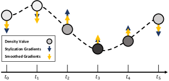
Figure 8. Particle density (circles) variation for a single particle over time. Temporal coherency is enforced by smoothing density gradients used for stylization from adjacent frames.

To further improve efficiency, and in contrast to TNST, we can keyframe stylizations, i.e., apply stylization to keyframes and interpolate particle attributes in-between. In practice, we reduced the stylization frames by a factor of 2 at max, but more drastic approximations could be used. Sparse keyframes still show temporally smooth transitions, but quality is degraded. Nevertheless, sparse keyframing would still be useful for generating quick previews of the simulation. The impact of sparse keyframing (every 10 frames) is shown in Figure 9.

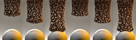
Figure 9. Stylization of every frame (left three images) versus keyframed stylization every 10 frames (images on the right). Sparse keyframing is visually similar and can be useful for quick previews.

5. Results

We implemented the method with the tensorflow framework and computed results on a TITAN Xp GPU (12GB). We used mantaflow [Thuerey and Pfaff, 2018] for smoke scene generation, a 3D smoke dataset from Kim et al. [2019a] for comparisons with TNST, a 2D smoke dataset from Jamriška et al. [2015] for color stylization, SPlisHSPlasH [Bender, 2016; Koschier et al., 2019] for liquid simulations and Houdini for rendering.

Performance

Using particles for stylization eliminates the need for recursively aligning stylization velocities from subsequent frames, which notably improves the computational performance. In combination with our sparse particle respesentation for smoke (1 particle per cell), simulations of size $200\times 300\times 200$ can now be stylized within an hour instead of a day (TNST). The computation time per frame is 0.66 minutes for the Smoke Jet scene shown in Figure 2, which is a speed-up of a factor of 20.41 compared to TNST. This improvement allows artists to more easily test different reference structures (input images) and hence renders neural flow stylization better applicable in production environments. Table (1) gives an overview of the timings and parameters for the individual test scenes. Keyframing (every other frame) was applied to the Smoke Jet (Figure 2) and Double Jets (Figure 12) examples.

Table 1. Performance table.

Scene	Resolution	# Particles	Time (m/f)
Moving Sphere (Fig. 10)	$192\times 192\times 192$	237K	0.8
Smoke Jet (Fig. 2)	$200\times 300\times 200$	1.2M	0.66
Double Jets (Fig. 12)	$200\times 200\times 200$	2M/2M	0.45
Chocolate (Fig. 13)	$200\times 200\times 200$	80K	0.05
Colored Smoke (Fig. 3)	$800\times 800$	136K	1.21
Dam Break (Fig. 14)	$512\times 1024$	23K	0.58
Double Dam (Fig. 15)	$512\times 1024$	31K/8K	0.65

Time-coherency

To illustrate the benefit of the Lagrangian formulation, we use a simple test scene where we initialize a smoke sphere with a uniform density. We then move the smoke artificially to the right, and apply the neural stylization to every frame of the sequence. We compare the results of LNST and TNST for different time instances in Figure 10. The top row shows the results of TNST. It can be seen that TNST is not able to preserve constant stylized textures in regions where the density function does not change. This is due to the recursive alignment of stylization gradients, which accumulate errors especially for bigger window sizes. The second row shows the corresponding results with LNST, demonstrating consistent stylization over time since gradients are constant. Also when applied a shearing deformation to the sphere, as shown in the third row, strucutures remain coherent. If an artist prefers to have changing structures in such situations, noise can be added to the densities carried by the particles, which in turn will induce stylization gradients as shown in the last row.

Figure 10. Selected frames of a stylized moving smoke sphere. From top to bottom: TNST with structures changing over time, LNST with temporally coherent structures, LNST result with applied shearing, and LNST result with noise-added density inducing style variation over time.

Smoke Stylization

Figure 2 shows a direct comparison of LNST and TNST applied to the smoke jet dataset of Kim et al. [2019a]. While the resulting structures inherently depend on the underlying representation, they naturally differ and cannot be directly compared with each other. It can be observed, however, that the Lagrangian stylization may lead to more pronounced structures, well visible in the semantic transfer net and the style transfer blue strokes, and that boundaries are smoother, noticeable in the Seated Nude example.

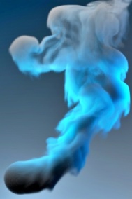
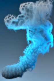
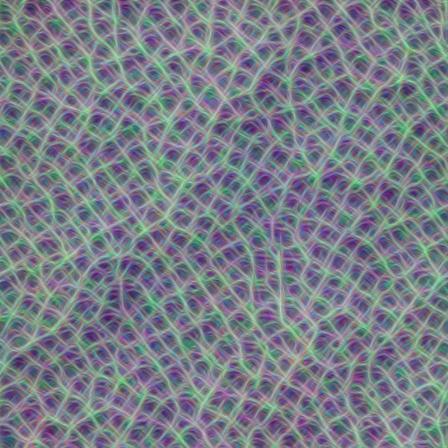
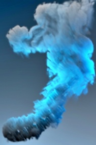
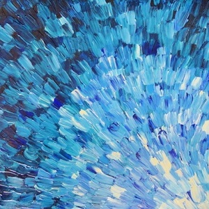
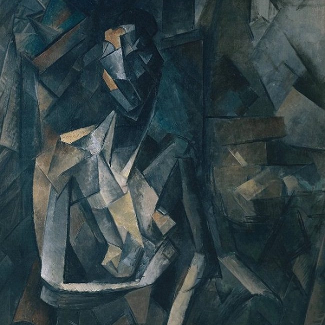
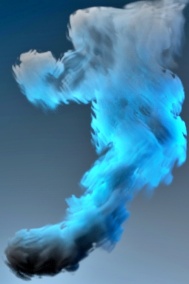
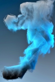
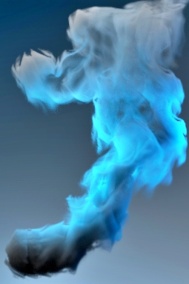
Figure 11. Semantic transfer applied to the smokejet simulation of [Kim et al., 2019a] (leftmost column). Stylized results are shown for our LNST (top) and TNST (bottom) for semantic feature transfer net (second column) and input images blue strokes, Seated Nude, and fire (last three columns).

Multi-fluid Stylization

Stylization of multiple fluids is naturally enabled by stylizing different sets of particles with different input images. Figure 12 shows a simulation of two smoke jets colliding, where the left one is stylized with the semantic feature net and the right one with the style transfer of the input image spirals. Transferred structures are retained per fluid type even if the flow undergoes complex mixing effects.

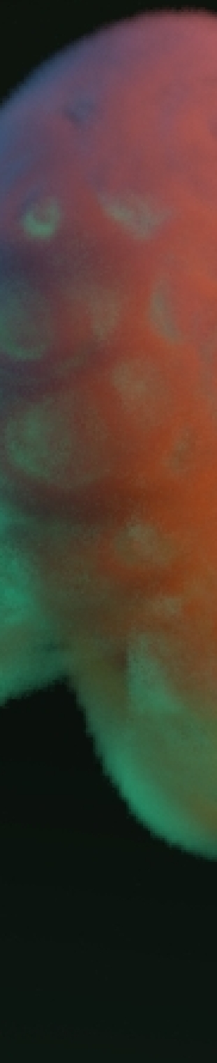
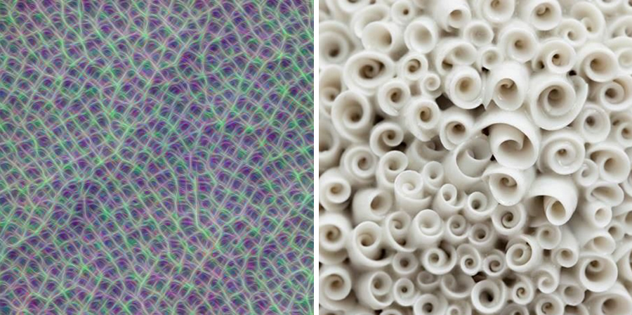
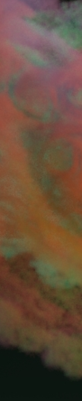
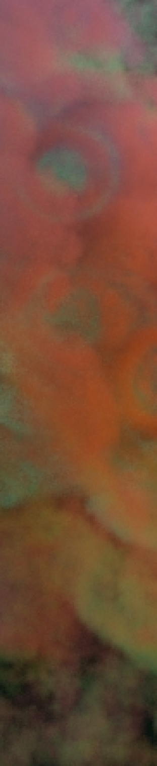
Figure 12. Two colliding smoke jets, which are stylized individually with the semantic feature net and input image spirals. The Lagrangian representation enables coherent stylization of multiple fluids even if the flow undergoes complex mixing.

Stylization of Liquids

We use a simple differentiable renderer for stylization of liquids. Unlike smoke renderer, which integrates media radiance scattered in the medium, we compute the amount of diffused light, i.e., absorbed light except transmitted by its liquid volume [Ihmsen et al., 2012], which is given by

(11) $$\begin{split}\tau(\mathbf{x},\mathbf{r})=e^{-\gamma\int_{\mathbf{0}}^{\mathbf{x}}d(\mathbf{r})\;dr}\\ I_{ij}=1-\tau(\mathbf{r}_{max},\mathbf{r}).\end{split}$$

Figure 13 shows the results of a stylized SPH simulation computed with SPlisHSPlasH [Bender, 2016]. We applied the patterns spiral and diagonal to a thin sheet simulation.

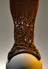
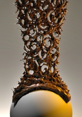
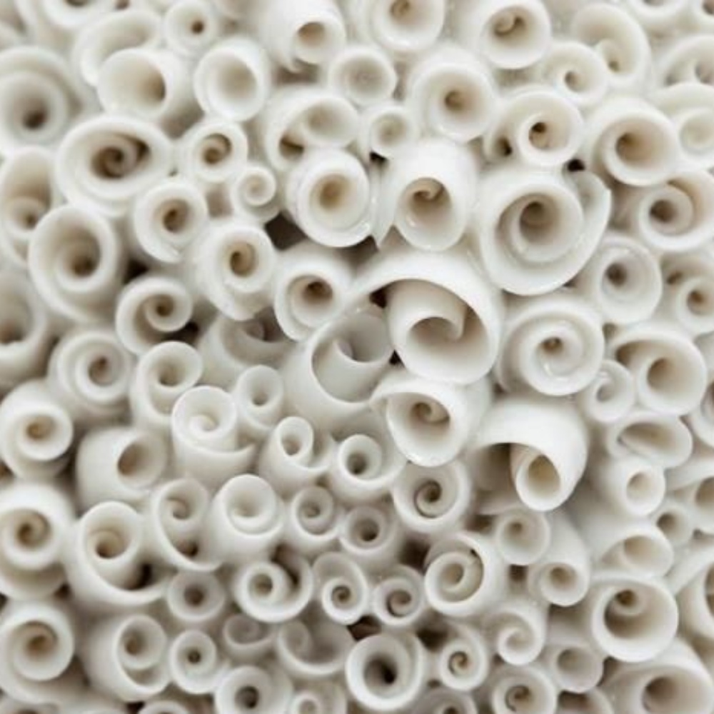
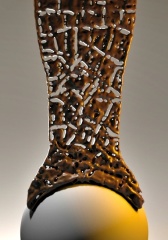
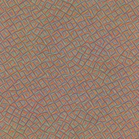
Figure 13. Thin sheet SPH simulation computed with SPlisHSPlasH [Bender, 2016] stylized with the patterns spiral and diagonal.

Color Transfer

We transfer color information from input images to flow fields by storing a color value per particle and optimizing it by Equation (7). This can be applied to any grid-based or particle-based smoke or liquid simulation. In Figure 14 we applied the color stylization to a 2D dam break simulation using different example images, and in Figure 15 to two liquids with distinct types (and hence color). The accompanying videos show that local color structures change very smoothly over time, which is attributed to the improved time-coherency of the Lagrangian stylization. This is especially well visible in Figure 3, where two subsequent frames are shown for TNST and LNST. In this example, we have transferred the style blue stroke to a smoke scene. The close-up views reveal discontinuities for TNST, while LNST shows smooth transitions for color structures.

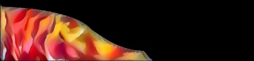
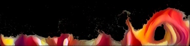
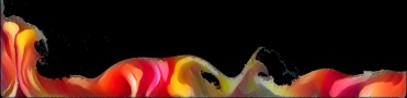
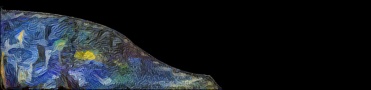
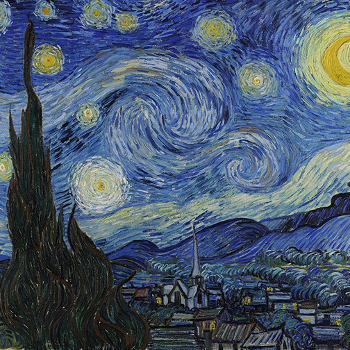
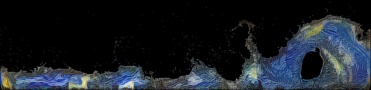
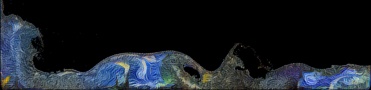
Figure 14. Lagrangian color stylization applied to a 2D particle-based liquid simulation using the input images Kanagawa Wave, Red Canna and Starry Night.

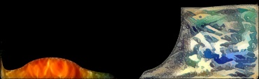
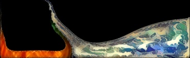
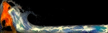
Figure 15. Lagrangian color stylization applied to a mixed 2D particle-based liquid simulation using the input images Kanagawa Wave and fire.

6. Discussion and Conclusion

We have presented a Lagrangian approach for neural flow stylization and have demonstrated benefits with respect to quality (improved temporal coherence), performance (stylization per frame in less than a minute), and art-directability (multi-fluid stylization, color transfer, liquid stylization). A key property of our approach is that it is not restricted to any particular fluid solver type (i.e., grids, particles, hybrid solvers). To enable this, we have introduced a strategy for grid-to-particle transfer (and vice versa) to efficiently update attributes and gradients, and a re-simulation that can be effectively applied to grid and particle fluid representations. This generality of our method facilitates seamless integration of neural style transfer into existing content production workflows.

A current limitation of the method is that we use a simple differentiable renderer for liquids. While this works well for some scenarios, a dedicated differentiable renderer for liquids would improve the resulting quality and especially also support a wider range of liquid simulation setups. Similar to the smoke renderer, such a liquid renderer must be differentiable as gradients are back-propagated in the optimization. It must also be efficient as the renderer is used in each step of the optimization. Although the complexity of the renderer has a direct influence on the quality of the results, we suspect that, analogously to our smoke renderer, a lightweight renderer that can recover the core flow structures is sufficient for stylizing liquids.

We have shown that LNST enables novel effects and a high degree of art-directability, which renders flow stylization more practical in prodcution workflows. However, we have not tested the method on large-scale simulations that are typically used in such settings. While our method can handle up to 2 million particles, larger scenes are restricted by the available memory. Moreover, in practical settings the scene complexity is higher, which potentially poses challenges with respect to artist control of the stylization.

By reducing the computation time for stylizing an entire simulation from one day with TNST to a single hour with LNST renders the method much more practical for digital artists. However, for testing different input structures, a real-time method would be desirable. Recent concepts presented on neural image stylization might be mapped to 3D simulations to further improve efficiency.

- [1]
- Ando et al. [2013] Ryoichi Ando, Nils Thürey, and Chris Wojtan. 2013. Highly adaptive liquid simulations on tetrahedral meshes. ACM Transactions on Graphics 32, 4 (jul 2013), 1.
- Ando and Tsuruno [2011] Ryoichi Ando and Reiji Tsuruno. 2011. A particle-based method for preserving fluid sheets. In Proceedings of SCA’11. 7. https://doi.org/10.1145/2019406.2019408
- Bargteil et al. [2006] Adam W Bargteil, Funshing Sin, Jonathan E Michaels, Tolga G Goktekin, and James F O’Brien. 2006. A Texture Synthesis Method for Liquid Animations. In Proceedings of SCA’06. 345–351. http://dl.acm.org/citation.cfm?id=1218064.1218111
- Becker and Teschner [2007] Markus Becker and Matthias Teschner. 2007. Weakly compressible SPH for free surface flows. In Symposium on Computer Animation. 1–8.
- Bender [2016] Jan Bender. 2016. SPlisHSPlasH. https://github.com/InteractiveComputerGraphics/SPlisHSPlasH.
- Bender and Koschier [2015] Jan Bender and Dan Koschier. 2015. Divergence-Free Smoothed Particle Hydrodynamics. In Symposium on Computer Animation. 1–9.
- Bi et al. [2017] Sai Bi, Nima Khademi Kalantari, and Ravi Ramamoorthi. 2017. Patch-based optimization for image-based texture mapping. ACM ToG 36, 4 (jul 2017), 1–11.
- Bousseau et al. [2007] Adrien Bousseau, Fabrice Neyret, Joëlle Thollot, and David Salesin. 2007. Video watercolorization using bidirectional texture advection. ACM ToG 26, 3 (2007).
- Brackbill et al. [1988] J.U. Brackbill, D.B. Kothe, and H.M. Ruppel. 1988. Flip: A low-dissipation, particle-in-cell method for fluid flow. Computer Physics Communications 48, 1 (1988), 25–38.
- Browning et al. [2014] Mark Browning, Connelly Barnes, Samantha Ritter, and Adam Finkelstein. 2014. Stylized keyframe animation of fluid simulations. In Proceedings of the Workshop on Non-Photorealistic Animation and Rendering. ACM, 63–70.
- Christen et al. [2019] Fabienne Christen, Byungsoo Kim, Vinicius C. Azevedo, and Barbara Solenthaler. 2019. Neural Smoke Stylization with Color Transfer. (dec 2019). arXiv:1912.08757 http://arxiv.org/abs/1912.08757
- Chu and Thuerey [2017] Mengyu Chu and Nils Thuerey. 2017. Data-driven synthesis of smoke flows with CNN-based feature descriptors. ACM Transactions on Graphics 36, 4 (jul 2017), 1–14.
- Desbrun and Gascuel [1996] Mathieu Desbrun and Marie-Paule Gascuel. 1996. Smoothed Particles: A new paradigm for animating highly deformable bodies. In Eurographics Workshop on Computer Animation and Simulation. 61–76.
- Diamanti et al. [2015] Olga Diamanti, Connelly Barnes, Sylvain Paris, Eli Shechtman, and Olga Sorkine-Hornung. 2015. Synthesis of Complex Image Appearance from Limited Exemplars. ACM Transactions on Graphics 34, 2 (mar 2015), 1–14.
- Ferstl et al. [2016] Florian Ferstl, Ryoichi Ando, Chris Wojtan, Rüdiger Westermann, and Nils Thuerey. 2016. Narrow Band FLIP for Liquid Simulations. CGF 35, 2 (2016), 225–232.
- Fišer et al. [2016] Jakub Fišer, Ondřej Jamriška, Michal Lukáč, Eli Shechtman, Paul Asente, Jingwan Lu, and Daniel Sýkora. 2016. StyLit: illumination-guided example-based stylization of 3D renderings. ACM ToG 35 (2016), 1–11. https://doi.org/10.1145/2897824.2925948
- Fu et al. [2017] Chuyuan Fu, Qi Guo, Theodore Gast, Chenfanfu Jiang, and Joseph Teran. 2017. A polynomial particle-in-cell method. ACM ToG 36, 6 (nov 2017), 1–12.
- Gagnon et al. [2016] Jonathan Gagnon, François Dagenais, and Eric Paquette. 2016. Dynamic lapped texture for fluid simulations. The Visual Computer 32, 6-8 (jun 2016), 901–909.
- Gagnon et al. [2019] Jonathan Gagnon, Julián E. Guzmán, Valentin Vervondel, François Dagenais, David Mould, and Eric Paquette. 2019. Distribution Update of Deformable Patches for Texture Synthesis on the Free Surface of Fluids. CGF 38, 7 (2019), 491–500.
- Gatys et al. [2015] Leon A Gatys, Alexander S Ecker, and Matthias Bethge. 2015. A neural algorithm of artistic style. Nature Communications (2015).
- Gatys et al. [2016] Leon A. Gatys, Alexander S. Ecker, and Matthias Bethge. 2016. Image Style Transfer Using Convolutional Neural Networks. In 2016 IEEE CVPR. 2414–2423.
- Gissler et al. [2019] C Gissler, A Peer, S Band, J Bender, and M Teschner. 2019. Interlinked sph pressure solvers for strong fluid-rigid coupling. ACM ToG 38, 1 (2019), 5:1–5:13.
- He et al. [2012] Xiaowei He, Ning Liu, Sheng Li, Hongan Wang, and Guoping Wang. 2012. Local Poisson SPH for Viscous Incompressible Fluids. CGF 31 (2012), 1948—-1958.
- Holl et al. [2020] Philipp Holl, Nils Thuerey, and Vladlen Koltun. 2020. Learning to Control PDEs with Differentiable Physics. In ICLR. https://openreview.net/forum?id=HyeSin4FPB
- Hu et al. [2020] Yuanming Hu, Luke Anderson, Tzu-Mao Li, Qi Sun, Nathan Carr, Jonathan Ragan-Kelley, and Fredo Durand. 2020. DiffTaichi: Differentiable Programming for Physical Simulation. In ICLR. https://openreview.net/forum?id=B1eB5xSFvr
- Hu et al. [2019a] Yuanming Hu, Jiancheng Liu, Andrew Spielberg, Joshua B Tenenbaum, William T Freeman, Jiajun Wu, Daniela Rus, and Wojciech Matusik. 2019a. ChainQueen: A real-time differentiable physical simulator for soft robotics. In ICRA. 6265–6271.
- Hu et al. [2019b] Yuanming Hu, Xinxin Zhang, Ming Gao, and Chenfanfu Jiang. 2019b. On hybrid lagrangian-eulerian simulation methods: practical notes and high-performance aspects. In ACM SIGGRAPH 2019 Courses. 16.
- Ihmsen et al. [2012] Markus Ihmsen, Nadir Akinci, Gizem Akinci, and Matthias Teschner. 2012. Unified spray, foam and air bubbles for particle-based fluids. The Visual Computer 28, 6-8 (2012), 669–677.
- Ihmsen et al. [2014] Markus Ihmsen, Jens Cornelis, Barbara Solenthaler, Christopher Horvath, and Matthias Teschner. 2014. Implicit incompressible SPH. IEEE TVCG 20, 3 (2014), 426–436.
- Insafutdinov and Dosovitskiy [2018] Eldar Insafutdinov and Alexey Dosovitskiy. 2018. Unsupervised Learning of Shape and Pose with Differentiable Point Clouds. In NeurIPS.
- Jamriška et al. [2015] Ondřej Jamriška, Jakub Fišer, Paul Asente, Jingwan Lu, Eli Shechtman, and Daniel Sýkora. 2015. LazyFluids: appearance transfer for fluid animations. ACM Transactions on Graphics (TOG) 34, 4 (2015), 92.
- Jiang et al. [2015] Chenfanfu Jiang, Craig Schroeder, Andrew Selle, Joseph Teran, and Alexey Stomakhin. 2015. The affine particle-in-cell method. ACM ToG 34, 4 (jul 2015), 51:1–51:10.
- Jiang et al. [2016] Chenfanfu Jiang, Craig Schroeder, Joseph Teran, Alexey Stomakhin, and Andrew Selle. 2016. The material point method for simulating continuum materials. In ACM SIGGRAPH 2016 Courses. 1–52.
- Jing et al. [2019] Yongcheng Jing, Yezhou Yang, Zunlei Feng, Jingwen Ye, Yizhou Yu, and Mingli Song. 2019. Neural style transfer: A review. IEEE TVCG (2019).
- Kato et al. [2018] Hiroharu Kato, Yoshitaka Ushiku, and Tatsuya Harada. 2018. Neural 3d mesh renderer. In Proceedings of the IEEE Conference on CVPR. 3907–3916.
- Kim et al. [2019a] Byungsoo Kim, Vinicius C. Azevedo, Markus Gross, and Barbara Solenthaler. 2019a. Transport-based neural style transfer for smoke simulations. ACM Transactions on Graphics 38, 6 (nov 2019), 1–11. https://doi.org/10.1145/3355089.3356560
- Kim et al. [2019b] Byungsoo Kim, Vinicius C. Azevedo, Nils Thuerey, Theodore Kim, Markus Gross, and Barbara Solenthaler. 2019b. Deep Fluids: A Generative Network for Parameterized Fluid Simulations. Computer Graphics Forum 38, 2 (2019).
- Kim et al. [2006] Janghee Kim, Deukhyun Cha, Byungjoon Chang, Bonki Koo, and Insung Ihm. 2006. Practical Animation of Turbulent Splashing Water. In Proceedings SCA’07. 335–344.
- Kim et al. [2013] Theodore Kim, Jerry Tessendorf, and Nils Thuerey. 2013. Closest point turbulence for liquid surfaces. ACM Transactions on Graphics (TOG) 32, 2 (2013), 15.
- Kim et al. [2008] Theodore Kim, Nils Thürey, Doug James, and Markus Gross. 2008. Wavelet turbulence for fluid simulation. In ACM Transactions on Graphics (TOG), Vol. 27. ACM, 50.
- Koschier and Bender [2017] D Koschier and J Bender. 2017. Density maps for improved sph boundary handling. In ACM SIGGRAPH/Eurographics Symposium on Computer Animation. 1–10.
- Koschier et al. [2019] Dan Koschier, Jan Bender, Barbara Solenthaler, and Matthias Teschner. 2019. Smoothed Particle Hydrodynamics Techniques for the Physics Based Simulation of Fluids and Solids. In Eurographics 2019 - Tutorials.
- Kwatra et al. [2006] Vivek Kwatra, David Adalsteinsson, Nipun Kwatra, Mark Carlson, and Ming C. Lin. 2006. Texturing fluids. In ACM SIGGRAPH ’06 Sketches on. 63.
- Kwatra et al. [2005] Vivek Kwatra, Irfan Essa, Aaron Bobick, and Nipun Kwatra. 2005. Texture optimization for example-based synthesis. In ACM SIGGRAPH ’05. 795.
- Ladický et al. [2015] L’ubor Ladický, SoHyeon Jeong, Barbara Solenthaler, Marc Pollefeys, and Markus Gross. 2015. Data-driven fluid simulations using regression forests. ACM Transactions on Graphics 34, 6 (oct 2015), 1–9. https://doi.org/10.1145/2816795.2818129
- Liu and Jacobson [2019] Hsueh-Ti Derek Liu and Alec Jacobson. 2019. Cubic Stylization. ACM ToG (2019).
- Liu et al. [2018] Hsueh-Ti Derek Liu, Michael Tao, and Alec Jacobson. 2018. Paparazzi: Surface Editing by way of Multi-View Image Processing. ACM Transactions on Graphics (2018).
- Loper and Black [2014] Matthew M. Loper and Michael J. Black. 2014. OpenDR: An Approximate Differentiable Renderer. 154–169. https://doi.org/10.1007/978-3-319-10584-0_11
- Losasso et al. [2008] F. Losasso, J.O. Talton, N. Kwatra, and R. Fedkiw. 2008. Two-Way Coupled SPH and Particle Level Set Fluid Simulation. IEEE TVCG 14, 4 (jul 2008), 797–804.
- Macklin and Mueller [2013] Miles Macklin and Matthias Mueller. 2013. Position Based Fluids. ACM Transactions on Graphics 32, 4 (2013), 104:1–104:12.
- McNamara et al. [2004] Antoine McNamara, Adrien Treuille, Zoran Popović, and Jos Stam. 2004. Fluid control using the adjoint method. In ACM SIGGRAPH ’04. 449.
- Monaghan [2005] J J Monaghan. 2005. Smoothed Particle Hydrodynamics. Reports on Progress in Physics 68, 8 (2005), 1703–1759.
- Müller et al. [2003] Matthias Müller, David Charypar, and Markus Gross. 2003. Particle-Based Fluid Simulation for Interactive Applications. In Symposium on Computer Animation.
- Narain et al. [2007] Rahul Narain, Vivek Kwatra, Huai-Ping Lee, Theodore Kim, Mark Carlson, and Ming C Lin. 2007. Feature-guided Dynamic Texture Synthesis on Continuous Flows. In Proceedings of the 18th EGSR. 361–370.
- Narain et al. [2008] Rahul Narain, Jason Sewall, Mark Carlson, and Ming C. Lin. 2008. Fast animation of turbulence using energy transport and procedural synthesis. ACM Transactions on Graphics 27, 5 (dec 2008), 1. https://doi.org/10.1145/1409060.1409119
- Nielsen and Bridson [2011] Michael B. Nielsen and Robert Bridson. 2011. Guide shapes for high resolution naturalistic liquid simulation. In ACM SIGGRAPH ’11. 1.
- Pan et al. [2013] Zherong Pan, Jin Huang, Yiying Tong, Changxi Zheng, and Hujun Bao. 2013. Interactive localized liquid motion editing. ACM ToG 32, 6 (nov 2013), 1–10.
- Pan and Manocha [2017] Zherong Pan and Dinesh Manocha. 2017. Efficient Solver for Spacetime Control of Smoke. ACM Trans. Graph. 36, 4, Article Article 68a (July 2017), 13 pages.
- Peer et al. [2015] A. Peer, M. Ihmsen, J. Cornelis, and M. Teschner. 2015. An Implicit Viscosity Formulation for SPH Fluids. ACM Transactions on Graphics 34, 4 (2015), 1–10.
- Pfaff et al. [2009] Tobias Pfaff, Nils Thuerey, Andrew Selle, and Markus Gross. 2009. Synthetic turbulence using artificial boundary layers. ACM Transactions on Graphics 28, 5 (dec 2009), 1.
- Raveendran et al. [2012] Karthik Raveendran, Nils Thuerey, Chris Wojtan, and Greg Turk. 2012. Controlling Liquids Using Meshes. In Proceedings of the SCA. 255–264.
- Reinhardt et al. [2019] Stefan Reinhardt, Tim Krake, Bernhard Eberhardt, and Daniel Weiskopf. 2019. Consistent Shepard Interpolation for SPH-Based Fluid Animation. ACM ToG 38 (2019).
- Ren et al. [2014] Bo Ren, Chenfeng Li, Xiao Yan, Ming C Lin, Javier Bonet, and Shi-Min Hu. 2014. Multiple-Fluid SPH Simulation Using a Mixture Model. ACM ToG 33, 5 (2014), 1–11.
- Sato et al. [2018] Syuhei Sato, Yoshinori Dobashi, Theodore Kim, and Tomoyuki Nishita. 2018. Example-based turbulence style transfer. ACM Trans. Graph. 37, 4 (2018), 84.
- Schechter and Bridson [2008] Hagit Schechter and Robert Bridson. 2008. Evolving Sub-Grid Turbulence for Smoke Animation. 1–7. https://doi.org/10.2312/SCA/SCA08/001-007
- Schenck and Fox [2018] Connor Schenck and Dieter Fox. 2018. SPNets: Differentiable Fluid Dynamics for Deep Neural Networks. In Conference on Robot Learning. 317–335.
- Servin et al. [2012] M. Servin, K. Bodin, and C. Lacoursiere. 2012. Constraint Fluids. IEEE TVCG 18, 03 (mar 2012), 516–526. https://doi.org/10.1109/TVCG.2011.29
- Solenthaler and Pajarola [2009] Barbara Solenthaler and Renato Pajarola. 2009. Predictive-corrective incompressible SPH. ACM Trans. Graph. 28, 3 (2009), 40:1–40:6.
- Stomakhin et al. [2013] Alexey Stomakhin, Craig Schroeder, Lawrence Chai, Joseph Teran, and Andrew Selle. 2013. A Material Point Method for Snow Simulation. ACM ToG 32, 4 (2013).
- Talmi et al. [2017] Itamar Talmi, Roey Mechrez, and Lihi Zelnik-Manor. 2017. Template matching with deformable diversity similarity. In Proceedings of the IEEE CVPR. 175–183.
- Thuerey [2016] Nils Thuerey. 2016. Interpolations of Smoke and Liquid Simulations. ACM Transactions on Graphics 36, 1 (sep 2016), 1–16. https://doi.org/10.1145/2956233
- Thuerey and Pfaff [2018] Nils Thuerey and Tobias Pfaff. 2018. MantaFlow. http://mantaflow.com.
- Tompson et al. [2017] Jonathan Tompson, Kristofer Schlachter, Pablo Sprechmann, and Ken Perlin. 2017. Accelerating eulerian fluid simulation with convolutional networks. In Proceedings of the 34th ICML-Volume 70. JMLR. org, 3424–3433.
- Treuille et al. [2003] Adrien Treuille, Antoine McNamara, Zoran Popović, and Jos Stam. 2003. Keyframe control of smoke simulations. ACM Transactions on Graphics 22, 3 (jul 2003), 716.
- Um et al. [2014] Kiwon Um, Seungho Baek, and JungHyun Han. 2014. Advanced Hybrid Particle-Grid Method with Sub-Grid Particle Correction. CGF 33, 7 (oct 2014), 209–218.
- Wiewel et al. [2019] Steffen Wiewel, Moritz Becher, and Nils Thuerey. 2019. Latent space physics: Towards learning the temporal evolution of fluid flow. In CGF, Vol. 38. 71–82.
- Xie et al. [2018] You Xie, Erik Franz, Mengyu Chu, and Nils Thuerey. 2018. tempogan: A temporally coherent, volumetric gan for super-resolution fluid flow. ACM ToG 37, 4 (2018).
- Yan et al. [2016] Xinchen Yan, Jimei Yang, Ersin Yumer, Yijie Guo, and Honglak Lee. 2016. Perspective transformer nets: Learning single-view 3d object reconstruction without 3d supervision. In Advances in NIPS. 1696–1704.
- Yang et al. [2016] Cheng Yang, Xubo Yang, and Xiangyun Xiao. 2016. Data-driven projection method in fluid simulation. CAVW 27, 3-4 (may 2016), 415–424.
- Yifan et al. [2019] Wang Yifan, Felice Serena, Shihao Wu, Cengiz Öztireli, and Olga Sorkine-Hornung. 2019. Differentiable Surface Splatting for Point-based Geometry Processing. (jun 2019). https://doi.org/10.1145/3355089.3356513 arXiv:1906.04173
- Yu et al. [2011] Q. Yu, F. Neyret, E. Bruneton, and N. Holzschuch. 2011. Lagrangian Texture Advection: Preserving both Spectrum and Velocity Field. IEEE TVCG 17, 11 (nov 2011).
- Zhu and Bridson [2005] Yongning Zhu and Robert Bridson. 2005. Animating sand as a fluid. ACM Transactions on Graphics 24, 3 (jul 2005), 965. https://doi.org/10.1145/1073204.1073298