Multi-Consensus Decentralized Accelerated Gradient Descent

Abstract

This paper considers the decentralized convex optimization problem, which has a wide range of applications in large-scale machine learning, sensor networks, and control theory. We propose novel algorithms that achieve optimal computation complexity and near optimal communication complexity. Our theoretical results give affirmative answers to the open problem on whether there exists an algorithm that can achieve a communication complexity (nearly) matching the lower bound depending on the global condition number instead of the local one. Furthermore, the linear convergence of our algorithms only depends on the strong convexity of global objective and it does not require the local functions to be convex. The design of our methods relies on a novel integration of well-known techniques including Nesterov’s acceleration, multi-consensus and gradient-tracking. Empirical studies show the outperformance of our methods for machine learning applications.

Keywords: consensus optimization, decentralized algorithm, accelerated gradient descent, gradient tracking, composite optimization

1 Introduction

In this paper, we consider the decentralized optimization problem, where the objective function is composed of $m$ local functions $f_{i}(x)$ that are located on $m$ different agents. The agents form a connected and undirected network and each of them only accesses its local function and communicates with its neighbors. All of the agents target to cooperatively solve the convex optimization problem

$$\min_{x\in\mathbb{R}^{d}}h(x)\triangleq f(x)+r(x)\quad\mbox{with}\quad f(x)\triangleq\frac{1}{m}\sum_{i=1}^{m}f_{i}(x),$$ (1)

where $f(x)$ is $L$-smooth and $\mu$-strongly convex, $r(x)$ is convex but may be non-differentiable. Many machine learning models have the form (1) such as logistic regression and elastic net regression. Decentralized optimization has been widely studied and applied in many applications such as large-scale machine learning (Tsianos et al., 2012; Kairouz et al., 2021), automatic control (Bullo et al., 2009; Lopes and Sayed, 2008), wireless communication (Ribeiro, 2010), and sensor networks (Rabbat and Nowak, 2004; Khan et al., 2009).

Many decentralized optimization algorithms have been proposed. One class of them is primal-only methods, including decentralized gradient methods (Nedic and Ozdaglar, 2009; Yuan et al., 2016), decentralized accelerated gradient method (Jakovetić et al., 2014; Qu and Li, 2019) and EXTRA (Shi et al., 2015b; Li et al., 2019; Mokhtari and Ribeiro, 2016). They only access the gradients of $f_{i}(x)$ and are usually computationally efficient. Another class of algorithms are the dual-based decentralized algorithms, such as the dual subgradient ascent (Terelius et al., 2011), dual gradient ascent and its accelerated version (Scaman et al., 2017; Uribe et al., 2020), the primal-dual method (Lan et al., 2020; Scaman et al., 2018; Hong et al., 2017), and ADMM (Erseghe et al., 2011; Shi et al., 2014). However, dual-based algorithms commonly need more computation cost when the gradient of the dual function is not explicitly available.

There are several important open problems in the area of decentralized optimization. First, Scaman et al. (2017, 2019) raised the problem whether there exists an algorithm that has a (near) optimal communication complexity depending on the global condition number $\kappa_{g}=L/\mu$ instead of the local condition number $\kappa_{\ell}$ (defined in Eq. (7)). Since the data distributed on different agents are potentially quite different, the global condition number $\kappa_{g}$ could be much smaller than $\kappa_{\ell}$. In the extreme case, the local function $f_{i}$ may be non-strongly convex, then it is possible that $\kappa_{\ell}$ is infinitely large while $\kappa_{g}$ is still small. However, existing works only achieved the optimal computation and communication complexities with respect to the local condition number $\kappa_{\ell}$ in the case of $r(x)=0$ (Kovalev et al., 2020; Li and Lin, 2021; Song et al., 2023; Scaman et al., 2017). Furthermore, it is unclear whether the convexity of each individual $f_{i}(x)$ is essential for computation-efficient and communication-efficient decentralized algorithms. Most of existing algorithms with linear convergence rates such as EXTRA (Shi et al., 2015b) and OPAC (Kovalev et al., 2020) all require each $f_{i}(x)$ to be (strongly) convex. Sun et al. (2022) first proposed the linear-convergent algorithm that allows some individual functions to be non-convex. However, Sun et al. (2022)’s algorithm cannot achieve the (near) optimal computation and communication complexities. Finally, existing methods cannot achieve the optimal computation and (near) optimal communication complexities for non-differentiable $r(x)$ (Xu et al., 2021; Alghunaim et al., 2020, 2019; Sun et al., 2022). How to design computation and communication efficient accelerated decentralized proximal gradient descent is still an open question.

This paper addresses the theoretical issues discussed above and designs two novel decentralized algorithms ProxMudag and Mudag. We summarize our contributions as follows:

1. Our algorithms have the optimal computation complexity $\mathcal{O}\left(\sqrt{\kappa_{g}}\log({1}/{\epsilon})\right)$ and the near optimal communication complexity $\mathcal{O}\big{(}\sqrt{{\kappa_{g}}/{(1-\lambda_{2}(W))}}\log\big{(}{M\kappa_{g}}/{L}\big{)}\log({1}/{\epsilon})\big{)}$, where $M$ and $L$ are the smoothness parameters of $f_{i}(x)$ and $f(x)$ respectively. To the best of our knowledge, this is the first (near) optimal decentralized algorithm that depends on the global condition number which provides an affirmative answer to the open problem whether there exists an algorithm that can achieve a communication complexity of $\mathcal{O}\left(\sqrt{{\kappa_{g}}/{(1-\lambda_{2}(W))}}\log({1}/{\epsilon})\right)$ or even close to it (Scaman et al., 2017).

2. Our algorithms do not require each individual function to be convex. Hence, they can be used in a wider range of applications than existing optimal decentralized algorithms. For example, the sub-problem of fast PCA by the shift-invert method is non-convex.

3. The proposed ProxMudag  can achieve optimal computation and (near) optimal communication complexity when $r(x)$ is convex but non-differentiable. To the best of our knowledge, it obtains the best-known communication complexity for the decentralized strongly-convex optimization problems with the composite objective function.

2 Related Work

We first review the penalty-based algorithms. Nedic and Ozdaglar (2009) proposed the well-known decentralized gradient descent method, where each agent performs a consensus step and a gradient descent step with a fixed step-size related to the penalty parameter. Yuan et al. (2016) proved the convergence rate of decentralized gradient descent and showed how the penalty parameter affects the computation complexity. To avoid the diminishing step-size commonly required in penalty-based algorithms, Jakovetić et al. (2014) combined multi-consensus and Nesterov’s acceleration to achieve the optimal computation complexity for minimizing non-strongly convex functions. Berahas et al. (2018) proposed to use multi-consensus to achieve the balance between computation and communication complexity. Recently, Li et al. (2020b) proposed APM-C, which employed multi-consensus and increased the penalty parameter properly for each iteration. Combining Nesterov’s acceleration, APM-C can achieve a linear convergence rate and a low communication complexity. Li et al. (2020a) applied multi-consensus to network Newton method to achieve computation and communication efficiency.

Dual-based methods are another important research line. These methods introduce a Lagrangian function and work in the dual space. There are different ways to solve the reformulated problem such as gradient descent method (Terelius et al., 2011), accelerated gradient method (Scaman et al., 2017; Uribe et al., 2020), primal-dual method (Lan et al., 2020; Scaman et al., 2018) and ADMM (Shi et al., 2014; Erseghe et al., 2011). However, such methods are typically computationally inefficient. For example, using the accelerated gradient method to solve the dual counterpart of the decentralized optimization problem can achieve optimal communication complexity Scaman et al. (2017); Uribe et al. (2020), but its computation complexity will have an additional dependency on the eigenvalue gap of gossip matrix (Uribe et al., 2020).

The gradient-tracking method is a popular way to reduce the computational cost (Qu and Li, 2017; Xu et al., 2015; Qu and Li, 2019; Di Lorenzo and Scutari, 2016, 2015; Sun et al., 2022; Nedic et al., 2017; Zhu and Martínez, 2010). There are two different techniques for gradient-tracking. One of them is keeping a variable to estimate the average gradient and uses this estimation in the gradient descent step (Sun et al., 2022; Di Lorenzo and Scutari, 2016; Qu and Li, 2017). Another one is introducing two different weight matrices to track the difference of gradients (Shi et al., 2015b; Li et al., 2019). Recently, (Nedic et al., 2017; Li and Lin, 2020; Jakovetić, 2018; Xu et al., 2021) studied the connection between these two strategies and showed that they can be transformed to each other. Due to the tracking of history information, gradient-tracking based algorithms can achieve linear convergence rates for strongly convex objective functions (Qu and Li, 2017; Shi et al., 2015b; Nedic et al., 2017; Sun et al., 2022). However, the previously obtained convergence rates and communication complexities are much worse than the results in this paper.

Methods	Computation	Communication	Is $f_{i}(x)$ convex?
Acc-DNGD (Qu and Li, 2019)	$\mathcal{O}\left(\frac{\kappa_{\ell}^{5/7}}{(1-\lambda_{2}(W))^{1.5}}\log\left(\frac{1}{\epsilon}\right)\right)$	$\mathcal{O}\left(\frac{\kappa_{\ell}^{5/7}}{(1-\lambda_{2}(W))^{1.5}}\log\left(\frac{1}{\epsilon}\right)\right)$	Yes
NIDS (Li et al., 2019)	$\mathcal{O}\left(\big{(}\kappa_{\ell}+\frac{1}{1-\lambda_{2}(W)}\big{)}\log\left(\frac{1}{\epsilon}\right)\right)$	$\mathcal{O}\left(\big{(}\kappa_{\ell}+\frac{1}{1-\lambda_{2}(W)}\big{)}\log\left(\frac{1}{\epsilon}\right)\right)$	Yes
ADA (Uribe et al., 2020)	$\mathcal{O}\left(\frac{\kappa_{\ell}}{\sqrt{1-\lambda_{2}(W)}}\log^{2}\frac{1}{\epsilon}\right)$	$\mathcal{O}\left(\sqrt{\frac{\kappa_{\ell}}{1-\lambda_{2}(W)}}\log\left(\frac{1}{\epsilon}\right)\right)$	Yes
APM-C Li et al. (2020b)	$\mathcal{O}\left(\sqrt{\kappa_{\ell}}\log\left(\frac{1}{\epsilon}\right)\right)$	$\mathcal{O}\left(\sqrt{\frac{\kappa_{\ell}}{1-\lambda_{2}(W)}}\log^{2}\frac{1}{\epsilon}\right)$	Yes
Acc-EXTRA (Li and Lin, 2020)	$\widetilde{\mathcal{O}}\left(\sqrt{\frac{\kappa_{\ell}}{1-\lambda_{2}(W)}}\log\left(\frac{1}{\epsilon}\right)\right)$	$\widetilde{\mathcal{O}}\left(\sqrt{\frac{\kappa_{\ell}}{1-\lambda_{2}(W)}}\log\left(\frac{1}{\epsilon}\right)\right)$	Yes
OPAC (Kovalev et al., 2020)	$\mathcal{O}\left(\sqrt{\kappa_{\ell}}\log\frac{1}{\epsilon}\right)$	$\mathcal{O}\left(\sqrt{\frac{\kappa_{\ell}}{1-\lambda_{2}(W)}}\log\frac{1}{\epsilon}\right)$	Yes
Mudag (Algorithm 1)	$\mathcal{O}\left(\sqrt{\kappa_{g}}\log\left(\frac{1}{\epsilon}\right)\right)$	$\widetilde{\mathcal{O}}\left(\sqrt{\frac{\kappa_{g}}{1-\lambda_{2}(W)}}\log\left(\frac{1}{\epsilon}\right)\right)$	No
Lower Bound (Scaman et al., 2017)	$\Omega\left(\sqrt{\kappa_{g}}\log\left(\frac{1}{\epsilon}\right)\right)$	$\Omega\left(\sqrt{\frac{\kappa_{g}}{1-\lambda_{2}(W)}}\log\left(\frac{1}{\epsilon}\right)\right)$

Table 1: Complexity comparisons between our algorithm and existing works for smooth and strongly convex problems. That is, $r(x)$ equals to zero in Problem (1). The notation $\mathcal{O}(\cdot)$ hides the constant terms and $\widetilde{\mathcal{O}}(\cdot)$ also hides $\log$ terms which are independent of $\epsilon$.

The communication complexities of existing works commonly depend on the local condition number $\kappa_{\ell}$ (Scaman et al., 2017; Li et al., 2020b, 2019; Li and Lin, 2021; Kovalev et al., 2020). Only EXTRA (Shi et al., 2015b) and DIGing (Nedic et al., 2017) achieve computation and communication complexities depending on $\hat{\kappa}_{g}$ (defined in Eq. (7)), which is still worse than our results that depend on $\kappa_{g}$ and $\log\hat{\kappa}_{g}$. Due to the fact $\kappa_{g}\leq\hat{\kappa}_{g}\leq m\kappa_{g}$, a communication complexity depending on $\kappa_{g}$ is preferred in real applications.

We summarize the results for the case of $r(x)=0$ in Table 1. Acc-DNGD is most relevant to our algorithm. It also utilizes Nesterov’s acceleration and gradient-tracking (Qu and Li, 2019). However, the multi-consensus step in our algorithm can analog the centralized accelerated gradient descent more efficiently and leads the convergence analysis almost to be the same as standard analysis (Nesterov, 2018) in the centralized scenario. In contrast, Acc-DNGD does not have such a good property and it does not achieve near optimal computation complexity nor near optimal communication complexity. Since our algorithm can effectively approximate the centralized accelerated gradient descent, our algorithm does not require each individual function $f_{i}(x)$ to be convex but only requires $f(x)$ to be strongly convex while this condition is required in Acc-DNGD. Finally, the convergence rate of our algorithm depends on the global condition number $\kappa_{g}$, while that of Acc-DNGD depends on the local condition number $\kappa_{\ell}$.

In Scaman et al. (2017), a lower bound of communication complexity was obtained for the decentralized optimization problem, which is $\mathcal{O}\big{(}\sqrt{{\kappa_{g}}/{(1-\lambda_{2}(W))}}\log({1}/{\epsilon})\big{)}$ for strongly convex problems. A dual-based algorithm was proposed to match the lower bound. However, this method is only suitable for the cases where dual functions of each local agent are easy to compute. Hence, the computation complexity of the method in Scaman et al. (2017) severely deteriorates once the dual functions are computationally inefficient to work with. Recently, Uribe et al. (2020) proposed an accelerated dual ascent algorithm which achieves the same communication complexity as the one of Scaman et al. (2017), but with a computation complexity of $\mathcal{O}\big{(}{\kappa_{\ell}}/{\sqrt{1-\lambda_{2}(W)}}\log^{2}({1}/{\epsilon})\big{)}$.

Recently, Li and Lin (2020) proposed Acc-EXTRA by applying Catalyst to accelerate EXTRA. However, due to the lack of the multi-consensus, Acc-EXTRA fails to achieve the optimal computation complexity. On the other hand, its communication complexity is also no better than Mudag. Furthermore, Catalyst introduces an additional loop of iteration. In contrast, Mudag is simple and easy to implement. Kovalev et al. (2020) proposed OPAC, which is a primal-dual based algorithm. The computation and communication complexities of OPAC are $\mathcal{O}\left(\sqrt{\kappa_{\ell}}\log({1}/{\epsilon})\right)$ and $\mathcal{O}\big{(}\sqrt{{\kappa_{\ell}}/{(1-\lambda_{2}(W))}}\log(1/\epsilon)\big{)}$ respectively, which depends on the local condition number. Additionally, it requires each $f_{i}(x)$ to be strongly convex.

Methods	Computation	Communication	Is $f_{i}(x)$ convex?
NIDS (Li et al., 2019)	$\mathcal{O}\left(\left(\kappa_{\ell}+\frac{1}{1-\lambda_{2}(W)}\right)\log\left(\frac{1}{\epsilon}\right)\right)$	$\mathcal{O}\left(\left(\kappa_{\ell}+\frac{1}{1-\lambda_{2}(W)}\right)\log\left(\frac{1}{\epsilon}\right)\right)$	Yes
D2P2 (Alghunaim et al., 2019)	$\mathcal{O}\left(\frac{\kappa_{\ell}}{1-\lambda_{2}(W)}\log\left(\frac{1}{\epsilon}\right)\right)$	$\mathcal{O}\left(\frac{\kappa_{\ell}}{1-\lambda_{2}(W)}\log\left(\frac{1}{\epsilon}\right)\right)$	Yes
ProxMudag (Algorithm 3)	$\mathcal{O}\left(\sqrt{\kappa_{g}}\log\left(\frac{1}{\epsilon}\right)\right)$	$\widetilde{\mathcal{O}}\left(\sqrt{\frac{\kappa_{g}}{1-\lambda_{2}(W)}}\log\left(\frac{1}{\epsilon}\right)\right)$	No

Table 2: Complexity comparisons between our algorithm and existing works for composite and strongly convex problems.

For the case $r(x)$ is convex but non-differentiable, many gradient tracking based algorithms have been extended to decentralized composite optimization problems with a non-differentiable regularization term such as PG-EXTRA (Shi et al., 2015a) and NIDS (Li et al., 2019). However, due to the non-differentiable term, these algorithms can only achieve sub-linear convergence rates. Recently, Sun et al. (2022) proposed a gradient tracking based method called SONATA, and established a linear convergence rate with the assumption that $f(x)$ is strongly convex. In addition, Alghunaim et al. (2019) proposed a primal-dual algorithm which can achieve a linear convergence rate when each $f_{i}(x)$ is convex. Recently, Alghunaim et al. (2020); Xu et al. (2021) proposed a unified framework to analyze a large group of algorithms. They showed the algorithms including EXTRA (PG-EXTRA) (Shi et al., 2015b), NIDS (Li et al., 2019) and Harnessing (Qu and Li, 2017) can also achieve linear convergence rates with a non-differentiable regularization term. Despite intensive studies in the literature, the convergence rates of these previous algorithms do not match the optimal convergence rate. Moreover, the communication complexities achieved by algorithms analyzed in the framework of Xu et al. (2021) and Alghunaim et al. (2020) are sub-optimal. The conference version of our paper proposed DAPG which achieves the optimal computation complexity and near optimal communication complexity (Ye et al., 2020). However DAPG takes three multi-consensus steps while ProxMudag in this paper only takes two multi-consensus steps. Thus, ProxMudag can achieve better communication-efficiency than DAPG. We compare our ProxMudag with existing state-of-the-art decentralized algorithms for the composite optimization in Table 2.

3 Preliminaries

We let $x_{i}\in\mathbb{R}^{d}$ be the local copy of the variable of $x$ for agent $i$ and we introduce the aggregate variable $\mathbf{x}\in\mathbb{R}^{m\times d}$, aggregate objective function $F(\mathbf{x})$ and aggregate gradient $\nabla F(\mathbf{x})\in\mathbb{R}^{m\times d}$ as

$$\mathbf{x}=\begin{bmatrix}x_{1}^{\top}\\ \vdots\\ x_{m}^{\top}\end{bmatrix},\quad F(\mathbf{x})=\frac{1}{m}\sum_{i=1}^{m}f_{i}(x_{i})\quad\text{and}\quad\nabla F(\mathbf{x})=\begin{bmatrix}\nabla f_{1}(x_{1})^{\top}\\ \vdots\\ \nabla f_{m}(x_{m})^{\top}\end{bmatrix}.$$ (2)

We denote that

$$\bar{x}_{t}=\frac{1}{m}\sum_{i=0}^{m}\mathbf{x}_{t}^{(i)},\quad\bar{y}_{t}=\frac{1}{m}\sum_{i=0}^{m}\mathbf{y}_{t}^{(i)}\quad\text{and}\quad\bar{g}_{t}=\frac{1}{m}\sum_{i=0}^{m}\nabla f_{i}(\mathbf{y}_{t}^{(i)}),$$ (3)

where $\mathbf{x}^{(i)}$ means the $i$-th row of matrix $\mathbf{x}$. Moreover, we use $\left\|\cdot\right\|$ to denote the Frobenius norm of vector or matrix and use $\left\langle x,y\right\rangle$ to denote the inner product of vectors $x$ and $y$.

Furthermore, we denote

$$R(\mathbf{x})=\frac{1}{m}\sum_{i=1}^{m}r(x_{i}).$$

Accordingly, we introduce the proximal operator and aggregated proximal operator with respect to $r(\cdot)$ and $R(\cdot)$ as

$$\small\begin{split}\!{\rm{\bf prox}}_{\eta,r}(x)=\mathop{\mathrm{argmin}}_{z\in\mathbb{R}^{d}}\Big{(}r(z)+\frac{1}{2\eta}\|z-x\|^{2}\Big{)}~{}~{}\text{and}~{}~{}{\rm{\bf prox}}_{m\eta,R}(\mathbf{x})=\mathop{\mathrm{argmin}}_{\mathbf{z}\in\mathbb{R}^{m\times d}}\Big{(}R(\mathbf{z})+\frac{1}{2m\eta}\|\mathbf{z}-\mathbf{x}\|^{2}\Big{)}.\end{split}$$ (4)

Using above notations, we define the (aggregated) generalized gradients as

$$G_{t}=\eta^{-1}\left(\mathbf{y}_{t}-{\rm{\bf prox}}_{\eta m,R}(\mathbf{y}_{t}-\eta\mathbf{s}_{t})\right)~{}~{}\mbox{and}~{}~{}G_{t}^{(i)}=\eta^{-1}\left(\mathbf{y}_{t}^{(i)}-{\rm{\bf prox}}_{\eta,r}(\mathbf{y}_{t}^{(i)}-\eta\mathbf{s}_{t}^{(i)})\right).$$ (5)

We also denote

$$\bar{G}_{t}=\frac{1}{m}\sum_{i=1}^{m}G_{t}^{(i)}.$$ (6)

Then we introduce the following definitions that will be used in the whole paper:

• We say $f(x)$ is $L$-smooth if for all $x,y\in\mathbb{R}^{d}$, it holds that

  $$f(y)\leq f(x)+\left\langle\nabla f(x),y-x\right\rangle+\frac{L}{2}\left\|y-x\right\|^{2}.$$

• We say $f(x)$ is $\mu$-strongly convex, if for all $x,y\in\mathbb{R}^{d}$, it holds that

  $$f(y)\geq f(x)+\left\langle\nabla f(x),y-x\right\rangle+\frac{\mu}{2}\left\|y-x\right\|^{2}.$$

• We say $f_{i}(x)$ is locally $M_{i}$-smooth if for all $x,y\in\mathbb{R}^{d}$, it holds that

  $$f_{i}(y)\leq f_{i}(x)+\left\langle\nabla f_{i}(x),y-x\right\rangle+\frac{M_{i}}{2}\left\|y-x\right\|^{2}.$$

• We say $f_{i}(x)$ is locally $\nu_{i}$-strongly convex if for all $x,y\in\mathbb{R}^{d}$, it holds that

  $$f_{i}(y)\geq f_{i}(x)+\left\langle\nabla f_{i}(x),y-x\right\rangle+\frac{\nu_{i}}{2}\left\|y-x\right\|^{2}.$$

Based on the smoothness and strong convexity, we can define global and local condition numbers of the objective function as

$$\kappa_{g}=\frac{L}{\mu},\qquad\hat{\kappa}_{g}=\frac{M}{\mu}\qquad\mbox{and}\qquad\kappa_{\ell}=\frac{M}{\nu},$$ (7)

where

$$M=\max_{i\in\{1,\dots,m\}}M_{i}\qquad\mbox{and}\qquad\nu=\min_{i\in\{1,\dots,m\}}\nu_{i}.$$ (8)

It is easy to verify that

$$L\leq M\qquad\mbox{and}\qquad\kappa_{g}\leq\hat{\kappa}_{g}\leq\kappa_{\ell}.$$ (9)

For the topology of the network, we let $W$ be the weight matrix associated with the network, indicating how agents are connected to each other. We assume that the weight matrix $W$ has the following properties:

1. $W$ is symmetric with $W_{i,j}\neq 0$ if and if only agents $i$ and $j$ are connected or $i=j$;

2. ${\mathbf{0}}\preceq W\preceq I$, $W{\mathbf{1}}={\mathbf{1}}$, ${\rm null}(I-W)={\rm span}(\mathbf{1})$;

where we use $I$ to denote the $m\times m$ identity matrix and ${\mathbf{1}}=[1,\dots,1]^{\top}\in\mathbb{R}^{m}$ denotes the vector with all ones. The weight matrix has an important property that $W^{\infty}=\frac{1}{m}\mathbf{1}\mathbf{1}^{\top}$ (Xiao and Boyd, 2004). Thus, one can achieve the effect of averaging local $x_{i}$ on different agents by using $W\mathbf{x}$ for iterations. Instead of directly multiplying $W$, Liu and Morse (2011) proposed a more efficient way to achieve averaging described in Algorithm 2, which has the following important proposition.

Proposition 1

Let $\mathbf{x}^{K}$ be the output of Algorithm 2 with $\eta_{w}=1/(1+\sqrt{1-\lambda_{2}^{2}(W)})$ and we denote $\bar{x}=\frac{1}{m}\mathbf{1}^{\top}\mathbf{x}^{0}$. Then it holds that

$$\bar{x}=\frac{1}{m}\mathbf{1}^{\top}\mathbf{x}^{K}\quad\mbox{and}\quad\left\|\mathbf{x}_{K}-\mathbf{1}\bar{x}\right\|\leq\sqrt{14}\left(1-\left(1-\frac{1}{\sqrt{2}}\,\right)\sqrt{1-\lambda_{2}(W)}\right)^{K}\left\|\mathbf{x}_{0}-\mathbf{1}\bar{x}\right\|,$$

where $\lambda_{2}(W)$ is the second largest eigenvalue of $W$.

Algorithm 1 Mudag

1:  Input: $x_{0}$, $\eta$, $\alpha$, and $K$

2:  Initialization: $\mathbf{x}_{0}=\mathbf{1}x_{0}$, $\mathbf{y}_{0}=\mathbf{x}_{0}$

3:  $\mathbf{x}_{1}=\mathrm{FastMix}(\mathbf{y}_{0}-\eta\nabla F(\mathbf{y}_{0}))$

4:  $\mathbf{y}_{1}=\mathbf{x}_{1}+\frac{1-\alpha}{1+\alpha}(\mathbf{x}_{1}-\mathbf{x}_{0})$

5:  for $t=1,\dots,T$ do

6:   $\mathbf{x}_{t+1}=\mathrm{FastMix}(\mathbf{y}_{t}+(\mathbf{x}_{t}-\mathbf{y}_{t-1})-\eta(\nabla F(\mathbf{y}_{t})-\nabla F(\mathbf{y}_{t-1})),\;K)$

7:   $\mathbf{y}_{t+1}=\mathbf{x}_{t+1}+\frac{1-\alpha}{1+\alpha}\left(\mathbf{x}_{t+1}-\mathbf{x}_{t}\right)$

8:  end for

9:  Output: $\mathbf{x}_{T}$

Algorithm 2 FastMix

1:  Input: $\mathbf{x}^{0}$, $K$, $W$ and $\eta_{w}$

2:  $\mathbf{x}^{-1}=\mathbf{x}^{0}$

3:  for $k=0,\dots,K$ do

4:   $\mathbf{x}^{k+1}=(1+\eta_{w})W\mathbf{x}^{k}-\eta_{w}\mathbf{x}^{k-1}$

5:  end for

6:  Output: $\mathbf{x}^{K}$

4 Multi-Consensus Decentralized Accelerated Gradient Descent

In this section, we propose two novel decentralized algorithms achieving the optimal computation complexity and near optimal communication complexity. These two algorithms are suitable for the case of $r(x)=0$ and the case of $r(x)$ is general convex respectively.

4.1 Algorithms and Main Ideas

Our algorithms are based on the multi-consensus, gradient-tracking and Nesterov’s acceleration technique. We first introduce ProxMudag (Algorithm 3) for solving the problem with $r(x)\neq 0$. It has the following algorithmic procedure:

$$\mathbf{x}_{t+1}= {\rm{\bf prox}}_{\eta m,R}(\mathbf{y}_{t}-\eta\mathbf{s}_{t}),$$ (10)

$$\mathbf{y}_{t+1}= \mathrm{FastMix}\left(\mathbf{x}_{t+1}+\frac{1-\alpha}{1+\alpha}(\mathbf{x}_{t+1}-\mathbf{x}_{t}),K\right),$$ (11)

$$\mathbf{s}_{t+1}= \mathrm{FastMix}(\mathbf{s}_{t}+\nabla F(\mathbf{y}_{t+1})-\nabla F(\mathbf{y}_{t}),\;K),$$ (12)

where $\eta$ is the step size and $K$ is the step number in multi-consensus. We can observe that Eqs. (10) and (11) belong to the algorithmic framework of accelerated proximal gradient descent since $\mathbf{s}_{t}$ can approximate the average gradient. In Eq. (12), we introduce $\mathbf{s}_{t}$ to track the gradient by using history information and the gradient difference. Thus, $\mathbf{s}_{t}$ can well approximate the average gradient $\mathbf{1}\bar{g}_{t}$ (defined in Eq. (3)). Furthermore, the variable $\mathbf{y}_{t}$ can also approximate $\mathbf{1}\bar{y}_{t}$ well by the “FastMix” operator. Since both $\bar{y}_{t}$ and $\bar{g}_{t}$ well approximate the averages, then we can obtain that $\bar{g}_{t}\approx\nabla f(\bar{y}_{t})$. Thus, the convergence properties of our algorithm are similar to the centralized accelerated proximal gradient descent, which is the main idea behind our approach to the decentralized optimization. In other words, we combine multi-consensus with gradient-tracking to approximate the centralized accelerated proximal gradient descent. As we will show, this seemingly simple idea leads to establishing a near optimal algorithm for the decentralized optimization. Note that Algorithm 3 only takes two multi-consensus steps at each iteration. In contrast, the algorithm in conference version (Ye et al., 2020, Algorithm 1) of this paper requires three multi-consensus steps at each round. Though reducing one multi-consensus step will not improve the order of communication complexity, it requires much less communication cost and benefits in real applications.

Algorithm 3 ProxMudag

1:  Input: $x_{0}$, $\eta$, $\alpha$, $K$

2:  Initialization: $\mathbf{x}_{0}=\mathbf{1}x_{0}$, $\mathbf{y}_{0}=\mathbf{x}_{0}$, $\mathbf{s}_{0}=\nabla F(\mathbf{x}_{0})$

3:  for $t=0,\dots,T$ do

4:   $\mathbf{x}_{t+1}={\rm{\bf prox}}_{\eta m,R}(\mathbf{y}_{t}-\eta\mathbf{s}_{t})$

5:   $\mathbf{y}_{t+1}=\mathrm{FastMix}\left(\mathbf{x}_{t+1}+\frac{1-\alpha}{1+\alpha}(\mathbf{x}_{t+1}-\mathbf{x}_{t}),K\right)$

6:   $\mathbf{s}_{t+1}=\mathrm{FastMix}(\mathbf{s}_{t}+\nabla F(\mathbf{y}_{t+1})-\nabla F(\mathbf{y}_{t}),\;K)$

7:  end for

8:  Output: $\mathbf{x}_{T}$

In the case of $r(x)=0$, we propose Mudag (Algorithm 1) that only needs one multi-consensus step for each iteration. The Mudag has the following algorithmic procedure:

$$\mathbf{x}_{t+1}= \mathrm{FastMix}(\mathbf{y}_{t}+(\mathbf{x}_{t}-\mathbf{y}_{t-1})-\eta(\nabla F(\mathbf{y}_{t})-\nabla F(\mathbf{y}_{t-1})),\;K),$$ (13)

$$\mathbf{y}_{t+1}= \mathbf{x}_{t+1}+\frac{1-\alpha}{1+\alpha}\left(\mathbf{x}_{t+1}-\mathbf{x}_{t}\right).$$

To understand Mudag from perspective of gradient tracking, we can reformulate the above procedure in a form similar to Eqs. (10) to (12) as follows (The reformulation is proved in Lemma 23)

$$\mathbf{x}_{t+1}= \mathrm{FastMix}\left(\mathbf{y}_{t}-\eta\mathbf{s}_{t},K\right),$$ (14)

$$\mathbf{y}_{t+1}= \mathbf{x}_{t+1}+\frac{1-\alpha}{1+\alpha}(\mathbf{x}_{t+1}-\mathbf{x}_{t}),$$ (15)

$$\mathbf{s}_{t+1}= \mathrm{FastMix}(\mathbf{s}_{t},K)+(\nabla F(\mathbf{y}_{t+1})-\nabla F(\mathbf{y}_{t}))-\eta^{-1}(\mathrm{FastMix}(\mathbf{y}_{t},K)-\mathbf{y}_{t}).$$ (16)

Note that Eq. (16) is an explicit gradient tracking step similar to Eq. (12). Comparing Eqs. (14)-(16) with Eqs. (10)-(12), we can observe that these two algorithms share a similar procedure since they share the same intuition. However, the iteration of ProxMudag cannot be improved to one multi-consensus step like Mudag. If we directly replace Eq. (13) by

$$\mathbf{x}_{t+1}= \mathrm{FastMix}\left({\rm{\bf prox}}_{\eta m,R}\left(\mathbf{y}_{t}+(\mathbf{x}_{t}-\mathbf{y}_{t-1})-\eta(\nabla F(\mathbf{y}_{t})-\nabla F(\mathbf{y}_{t-1}))\right),\,K\right),$$

it is easy to check that the algorithm cannot converge to the optimum.

Because Mudag only has one multi-consensus step for each iteration while ProxMudag takes two multi-consensus steps, in practice, Mudag commonly requires much less communication cost than ProxMudag when Mudag is applicable. Thus, the Mudag is a better choice than ProxMudag in the case of $r(x)=0$.

4.2 Main Results

In this work, we focus on the synchronized setting in which the computation complexity depends on the number of gradient calls and the communication complexity depends on the rounds of local communication. We give the detailed upper complexity bounds for our algorithms in the following theorems.

Theorem 2

Let $f(x)$ be $L$-smooth and $\mu$-strongly convex. Assume each $f_{i}(x)$ is $M$-smooth. We set $\eta={1}/{L}$ and $\alpha=\sqrt{\mu\eta}$ in Algorithm 1. Letting $K$ in Algorithm 1 satisfy that

$$K=\frac{\sqrt{2}}{\sqrt{2}-1}\sqrt{\frac{1}{1-\lambda_{2}(W)}}\log\left(\frac{\sqrt{14}}{\rho}\right)\qquad\mbox{with}\qquad\rho\leq\frac{1}{4^{3}\cdot 9\cdot 288}\cdot\left(\frac{L}{M}\right)^{4}\kappa_{g}^{-3},$$

then the sequence $\{\bar{x}_{t}\}$ satisfies that

$$\small\begin{split}f(\bar{x}_{T})-f(x^{*})\leq\left(1-\frac{\alpha}{2}\right)^{T}\left(f(\bar{x}_{0})-f(x^{*})+\frac{\mu\left\|\bar{x}_{0}-x^{*}\right\|^{2}}{2}+\frac{\mu}{288m}\sum_{i=1}^{m}\left\|\nabla f_{i}(\bar{x}_{0})-\nabla f(\bar{x}_{0})\right\|^{2}\right),\end{split}$$

where $x^{*}$ is the global minimum of $f(x)$. To achieve $\mathbf{x}_{T}$ such that $\left\|\mathbf{x}_{T}-\mathbf{1}x^{*}\right\|^{2}=\mathcal{O}(m\epsilon/\mu)$ and $f(\bar{x}_{T})-f(x^{*})\leq\epsilon$, the computation and communication complexities of Algorithm 1 are at most

$$T=\mathcal{O}\left(\sqrt{\kappa_{g}}\log\left(\frac{1}{\epsilon}\right)\right)\qquad\mbox{and}\qquad Q=\mathcal{O}\left(\sqrt{\frac{\kappa_{g}}{1-\lambda_{2}(W)}}\log\left(\frac{M\kappa_{g}}{L}\right)\log\left(\frac{1}{\epsilon}\right)\right)$$

respectively.

Theorem 3

Let $f(x)$ be $L$-smooth and $\mu$-strongly convex. Assume each $f_{i}(x)$ is $M$-smooth. We set $\eta={1}/{(2L)}$ and $\alpha=\sqrt{\mu\eta}$ in Algorithm 3. Letting $K$ in Algorithm 3 satisfy that

$$K=\frac{\sqrt{2}}{\sqrt{2}-1}\sqrt{\frac{1}{1-\lambda_{2}(W)}}\log\left(\frac{\sqrt{14}}{\rho}\right)\qquad\mbox{with}\qquad\rho\leq\frac{1}{5.5\cdot 10^{8}}\cdot\left(\frac{L}{M}\right)^{6}\kappa_{g}^{-3/2},$$

then sequence $\{\bar{x}_{t}\}$ generated by Algorithm 3 satisfies that

$$\small\begin{split}h(\bar{x}_{T})-h(x^{*})\leq\left(1-\frac{\alpha}{2}\right)^{T}\left(h(\bar{x}_{0})-h(x^{*})+\frac{\mu\left\|\bar{x}_{0}-x^{*}\right\|^{2}}{2}+\frac{52L}{m}\sum_{i}^{m}\left\|\nabla f_{i}(\bar{x}_{0})-\nabla f(\bar{x}_{0})\right\|^{2}\right),\end{split}$$

where $x^{*}$ is the global minimum of $h(x)$. To achieve $\mathbf{x}_{T}$ such that $\left\|\mathbf{x}_{T}-\mathbf{1}x^{*}\right\|^{2}=\mathcal{O}(m\epsilon/\mu)$ and $h(\bar{x}_{T})-h(x^{*})\leq\epsilon$, the computation and communication complexities of Algorithm 1 are at most

$$T=\mathcal{O}\left(\sqrt{\kappa_{g}}\log\left(\frac{1}{\epsilon}\right)\right)\qquad\mbox{and}\qquad Q=\mathcal{O}\left(\sqrt{\frac{\kappa_{g}}{1-\lambda_{2}(W)}}\log\left(\frac{M\kappa_{g}}{L}\right)\log\left(\frac{1}{\epsilon}\right)\right)$$

respectively.

Remark 4

Theorem 2 shows that Mudag  achieves the same order of computation complexity as that of the centralized Nesterov’s accelerated gradient descent. At the same time, the communication complexity nearly matches the known lower bound of decentralized optimization problem up to a factor of $\log\left({M\kappa_{g}}/{L}\right)$. We conjecture that it may be possible to remove the $\log(\kappa_{g})$ factor, because the term only comes from the inequality $\left\|\bar{y}_{t}-x^{*}\right\|\leq\sqrt{2V_{t}/{\mu}}$, where $V_{t}$ is defined in Eq. (17) in the proof, which may be loose.

Remark 5

Theorem 2 and 3 only assume that $f(x)$ is $\mu$-strongly convex and $L$-smooth, and $f_{i}(x)$ is $M$-smooth (note that unlike many previous works, our dependency on $M$ is logarithmic only). Thus, our algorithms can be used when $f_{i}(x)$ is possibly non-convex. This kind of problem has been widely studied in recent years (Allen-Zhu, 2018; Garber et al., 2016) and one important example is the fast PCA by shift-invert method (Garber et al., 2016). In contrast, the previous works (Scaman et al., 2017; Li et al., 2020b, 2019; Qu and Li, 2019; Kovalev et al., 2020; Li and Lin, 2021) require the (strong) convexity of $f_{i}(x)$ to obtain the linear convergence rate.

Remark 6

The computation and communication complexities of our algorithms depend on $\sqrt{\kappa_{g}}$ rather than $\sqrt{\kappa_{\ell}}$, which is a novel result. Before our work, it was unknown whether there exists a decentralized algorithm that can achieve a communication complexity close to the lower bound $\Omega\left(\sqrt{{\kappa_{g}}/{(1-\lambda_{2}(W))}}\log({1}/{\epsilon})\right)$ (Scaman et al., 2017, 2019).

Remark 7

Observe that the step 3 of Algorithm 1 resorts to multi-consensus and gradient tracking to encourage $\mathbf{x}(i,:)$ on different agents to be close to each other. Similarly, for the centralized distributed optimization problem, the consensus step is also needed, which is often implemented by two rounds of communications between agents and the central server. In this view, the centralized optimization methods and the decentralized one only differ in the way to achieve consensus. We can also regard the decentralized optimization methods as an approximation to the decentralized one.

5 Convergence Analysis

In this section, we give a detailed characterization on how our decentralized algorithms approximate accelerated (proximal) gradient descent. Since Mudag  and ProxMudag  have similar ideas for convergence analysis, we only present how to obtain the convergence rate of ProxMudag  in this section and leave the analysis of Mudag in Appendix C. Note that the analysis of ProxMudag may be more sophisticated than the one of Mudag because of the additional step of proximal operation.

We first introduce the Lyapunov function as follows

$$V_{t}=h(\bar{x}_{t})-h(x^{*})+\frac{\mu}{2}\left\|\bar{v}_{t}-x^{*}\right\|^{2},$$ (17)

where $\bar{v}_{t}$ is defined as

$$\bar{v}_{t}=\bar{x}_{t-1}+\frac{1}{\alpha}(\bar{x}_{t}-\bar{x}_{t-1})\quad\mbox{with}\qquad\alpha=\sqrt{\mu\eta}.$$ (18)

In the rest of this section, we will show how the Lyapunov function $V_{t}$ converges and how multi-consensus and gradient-tracking help us to approximate centralized accelerated proximal gradient descent.

Then we show that $\bar{x}_{t}$, $\bar{y}_{t}$, $\bar{g}_{t}$ (defined in Eq. (3) and generated by Algorithm 3) and $\bar{v}_{t}$ (defined in Eq. (18)) can be fit into the framework of the centralized accelerated proximal gradient descent.

Lemma 8

Let $\bar{x}_{t}$, $\bar{y}_{t}$, $\bar{g}_{t}$ and $\bar{G}_{t}$ (defined in Eqs. (3) and (6)) be generated by Algorithm 3. By setting $\bar{s}_{t}=\frac{1}{m}\mathbf{1}^{\top}\mathbf{s}_{t}$ with $\mathbf{s}_{t}$ defined in Eq. (12), it satisfies:

$$\bar{x}_{t+1}= \bar{y}_{t}-\eta\bar{G}_{t},$$ (19)

$$\bar{y}_{t+1}= \bar{x}_{t+1}+\frac{1-\alpha}{1+\alpha}(\bar{x}_{t+1}-\bar{x}_{t}),$$ (20)

$$\bar{s}_{t+1}= \bar{s}_{t}+\bar{g}_{t+1}-\bar{g}_{t}=\bar{g}_{t+1}.$$ (21)

Proof  Proposition 1 provides a property of FastMix that $\bar{x}=\frac{1}{m}\mathbf{1}^{\top}\mathrm{FastMix}(\mathbf{x},K)$. Combining the algorithmic procedures of Algorithm 3 and the definition of $\bar{G}_{t}$ in Eq. (6), we can obtain the first two equations.

We first the last equality by induction. For $t=0$, we use the fact that $\mathbf{s}_{0}=\nabla F(\mathbf{y}_{0})$. Then, it holds that $\bar{s}_{0}=\bar{g}_{0}$. We assume that $\bar{s}_{t}=\bar{g}_{t}$ at time $t$. By the update equation (12) and Proposition 1, we have

$$\bar{s}_{t+1}=\bar{s}_{t}+(\bar{g}_{t+1}-\bar{g}_{t})=\bar{g}_{t+1}.$$

Thus, we obtain the result at time $t+1$.  

Lemma 8 shows that the averaged version of Eqs. (10)-(12) is almost the same as accelerated proximal gradient descent (Nesterov, 2018). Thus, if $\bar{s}_{t}$ is an accurate estimation of $\nabla f(\bar{y}_{t})$, then Algorithm 3 has convergence properties similar to accelerated proximal gradient descent. Next, we are going to show $\mathbf{y}_{t}(i,:)\approx\bar{y}_{t}$ and $\mathbf{s}_{t}(i,:)\approx\bar{s}_{t}$ by the following lemma.

Lemma 9

Let $\mathbf{z}_{t}=[\left\|\mathbf{x}_{t}-\mathbf{1}\bar{x}_{t}\right\|,\left\|\mathbf{y}_{t}-\mathbf{1}\bar{y}_{t}\right\|,\eta\left\|\mathbf{s}_{t}-\mathbf{1}\bar{s}_{t}\right\|]^{\top}$ with $\mathbf{x}_{t}$, $\mathbf{y}_{t}$ and $\mathbf{s}_{t}$ generated by Algorithm 3, then it holds that

$$\mathbf{z}_{t+1}\leq\mathbf{A}\mathbf{z}_{t}+\frac{4\rho\sqrt{m}M}{L}\left[0,0,\sqrt{\frac{2V_{t}}{\mu}}\,\right]^{\top},$$ (22)

where $\rho$ and $\mathbf{A}$ are defined as

$$\rho=\left(1-\sqrt{1-\lambda_{2}(W)}\,\right)^{K}\quad\text{and}\quad\mathbf{A}=\begin{bmatrix}0&2&2\\ 2\rho&4\rho&4\rho\\ \rho M/L&8\rho M^{2}/L^{2}&5\rho M/L\end{bmatrix}.$$ (23)

If the spectral radius of $\mathbf{A}$ is less than $1$ and $V_{t}$ converges to zero, then $\left\|\mathbf{z}_{t}\right\|$ will converge to zero. Note that $\left\|\mathbf{x}_{t}-\mathbf{1}\bar{x}_{t}\right\|$, $\left\|\mathbf{y}_{t}-\mathbf{1}\bar{y}_{t}\right\|$ and $\eta\left\|\mathbf{s}_{t}-\mathbf{1}\bar{s}_{t}\right\|$ are no larger than $\left\|\mathbf{z}_{t}\right\|$. Hence, Algorithm 3 can well approximate centralized accelerated proximal gradient descent in such conditions.

Next, we prove above two conditions that lead to the convergence of $\left\|\mathbf{z}_{t}\right\|$. First, the following lemma shows the spectral radius of $\mathbf{A}$ is less than $\frac{1}{2}$ if $\rho$ is small enough.

Lemma 10

Matrix ${\mathbf{A}}$ defined in Eq. (23) satisfies that

$$0<\lambda_{1}(\mathbf{A})\qquad\text{and}\qquad|\lambda_{3}(\mathbf{A})|\leq|\lambda_{2}(\mathbf{A})|<\lambda_{1}(\mathbf{A})$$

with $\lambda_{i}(\mathbf{A})$ being the $i$-th largest eigenvalue of $\mathbf{A}$. Letting $\eta=1/(2L)$ and $\rho\leq{L^{3}}/{(1280M^{3})}$, then it holds that

$$\lambda_{1}({\mathbf{A}})\leq\frac{1}{2},$$

and the eigenvector $\mathbf{v}$ associated with $\lambda_{1}(\mathbf{A})$ is positive and its entries satisfy

$$0<\mathbf{v}(1)\leq\frac{8\mathbf{v}(3)}{\sqrt{\rho}},\qquad 0<\mathbf{v}(2)\leq 3\mathbf{v}(3)\qquad\text{and}\quad 0<\mathbf{v}(3),$$ (24)

where $\mathbf{v}(i)$ is $i$-th entry of $\mathbf{v}$.

Now, we are going to show $V_{t}$ converges linearly but with some perturbation terms related to $\mathbf{z}_{t}$.

Lemma 11

Letting $\mathbf{x}_{t},\mathbf{y}_{t},\mathbf{s}_{t}$ be generated by Algorithm 3, it holds that

$$V_{t+1}\leq(1-\alpha)V_{t}+\frac{13\eta}{m}\left\|\mathbf{s}_{t}-\mathbf{1}\bar{s}_{t}\right\|^{2}+\frac{20M^{2}\eta+10\eta^{-1}}{m}\left\|\mathbf{y}_{t}-\mathbf{1}\bar{y}_{t}\right\|^{2}.$$ (25)

The above lemma shows that the Algorithm 3 has a convergence property similar to the accelerated proximal gradient descent but with some perturbation terms. Next, using above lemmas and choosing proper $\rho$ by a proper $K$, we will obtain the convergence rate of Algorithm 3.

Finally, we provide the proof of our main result Theorem 3.

Proof It is easy to check that $\rho$ satisfies the conditions required in Lemma 10. Let the eigenvector $\mathbf{v}$ defined in Lemma 10 and set $\mathbf{v}(3)=1$. Combining with the fact that the first two entries of $\mathbf{z}_{0}$ are zero, we can obtain that,

$$\mathbf{z}_{0}\leq\left\|\mathbf{z}_{0}\right\|\mathbf{v}\qquad\mbox{and}\qquad[0,0,1]^{\top}\leq\mathbf{v}.$$

By Eq. (22), we can obtain that

$$\mathbf{z}_{t+1}\leq \left\|\mathbf{z}_{0}\right\|\cdot\mathbf{A}^{t+1}\mathbf{v}+\frac{4\rho M}{L}\sqrt{\frac{2m}{\mu}}\cdot\sum_{i=0}^{t}\sqrt{V_{i}}\cdot\mathbf{A}^{t-i}\mathbf{v}$$ (26)

$$= \left\|\mathbf{z}_{0}\right\|\lambda_{1}(\mathbf{A})^{t+1}\mathbf{v}+\frac{4\rho M}{L}\sqrt{\frac{2m}{\mu}}\cdot\sum_{i=0}^{t}\sqrt{V_{i}}\cdot\lambda_{1}(\mathbf{A})^{t-i}\mathbf{v}$$

$$\leq \left\|\mathbf{z}_{0}\right\|\left(\frac{1}{2}\right)^{t+1}\mathbf{v}+\frac{4\rho M}{L}\sqrt{\frac{2m}{\mu}}\cdot\sum_{i=0}^{t}\left(\frac{1}{2}\right)^{t-i}\sqrt{V_{i}}\cdot\mathbf{v},$$

where the first equality is because $\mathbf{v}$ is the eigenvector associated with $\lambda_{1}(\mathbf{A})$ and the last inequality is because of $\lambda_{1}(\mathbf{A})\leq\frac{1}{2}$ obtained in Lemma 10.

Next, we will prove our result by induction. For $t=0$, we have $\left\|\mathbf{y}_{0}-\mathbf{1}\bar{y}_{0}\right\|=0$ and

$$V_{1}\stackrel{{\scriptstyle\eqref{eq:VV}}}{{\leq}} (1-\alpha)V_{0}+\frac{13\eta^{-1}}{m}(\eta\left\|\mathbf{s}_{0}-\mathbf{1}\bar{s}_{0}\right\|)^{2}=(1-\alpha)V_{0}+\frac{13\eta^{-1}}{m}\left\|\mathbf{z}_{0}\right\|^{2}$$

$$\leq (1-\alpha)V_{0}+\left(1-\frac{\alpha}{2}\right)\frac{52L}{m}\left\|\mathbf{z}_{0}\right\|^{2}\leq\left(1-\frac{\alpha}{2}\right)\left(V_{0}+\frac{52L}{m}\left\|\mathbf{z}_{0}\right\|^{2}\right).$$

Next, we assume that for $i=1,\dots,t$, it holds that

$$V_{i}\leq\left(1-\frac{\alpha}{2}\right)^{i}\left(V_{0}+\frac{52L}{m}\left\|\mathbf{z}_{0}\right\|^{2}\right).$$ (27)

Combining with Eq. (26), we can obtain that

$$\mathbf{z}_{t-1}$$ (28)

$$\leq \mathbf{v}\cdot\left(4\rho\frac{M}{L}\sqrt{\frac{2m}{\mu}}\sum_{j=0}^{t-2}2^{-(t-2-j)}\sqrt{V_{j}}+2^{-(t-1)}\left\|\mathbf{z}_{0}\right\|\right)$$

$$\leq \mathbf{v}\cdot\left(4\rho\frac{M}{L}\sqrt{\frac{2m}{\mu}}\sum_{j=0}^{t-2}2^{-(t-2-j)}\left(\sqrt{1-\frac{\alpha}{2}}\right)^{j}\sqrt{V_{0}+\frac{52L}{m}\left\|\mathbf{z}_{0}\right\|^{2}}+2^{-(t-1)}\left\|\mathbf{z}_{0}\right\|\right)$$

$$= \mathbf{v}\cdot\left(4\rho\frac{M}{L}\sqrt{\frac{2m}{\mu}}\frac{2\left(\sqrt{1-\frac{\alpha}{2}}\right)^{t-1}-2^{-(t-2)}}{2\sqrt{1-\frac{\alpha}{2}}-1}\sqrt{V_{0}+\frac{52L}{m}\left\|\mathbf{z}_{0}\right\|^{2}}+2^{-(t-1)}\left\|\mathbf{z}_{0}\right\|\right)$$

$$\leq \mathbf{v}\cdot\left(12\frac{M}{L}\sqrt{\frac{2m}{\mu}}\left(\sqrt{1-\frac{\alpha}{2}}\right)^{t-1}\sqrt{V_{0}+\frac{52L}{m}\left\|\mathbf{z}_{0}\right\|^{2}}+2^{-(t-1)}\left\|\mathbf{z}_{0}\right\|\right).$$

Thus, using the definition of $\mathbf{z}$ and $\mathbf{A}$, we can obtain that

$$\left\|\mathbf{y}_{t}-\mathbf{1}\bar{y}_{t}\right\|$$

$$\stackrel{{\scriptstyle\eqref{eq:zaz}}}{{\leq}} \left\langle[2\rho,4\rho,4\rho],\mathbf{z}_{t-1}\right\rangle$$

$$\overset{\eqref{eq:z}}{\leq} \left\langle[2\rho,4\rho,4\rho],\mathbf{v}\right\rangle\cdot\left(\frac{12M}{L}\sqrt{\frac{2m}{\mu}}\left(\sqrt{1-\frac{\alpha}{2}}\right)^{t-1}\sqrt{V_{0}+\frac{52L}{m}\left\|\mathbf{z}_{0}\right\|^{2}}+2^{-(t-1)}\left\|\mathbf{z}_{0}\right\|\right)$$

$$\leq \rho\left(2\mathbf{v}(1)+4\mathbf{v}(2)+4\right)\cdot\left(\frac{12M}{L}\sqrt{\frac{2m}{\mu}}\left(\sqrt{1-\frac{\alpha}{2}}\right)^{t-1}\sqrt{V_{0}+\frac{52L}{m}\left\|\mathbf{z}_{0}\right\|^{2}}+2^{-(t-1)}\left\|\mathbf{z}_{0}\right\|\right)$$

$$\stackrel{{\scriptstyle\eqref{eq:v_v}}}{{\leq}} \rho\cdot\left(\frac{16}{\sqrt{\rho}}+12+4\right)\cdot\left(\frac{12M}{L}\sqrt{\frac{2m}{\mu}}\left(\sqrt{1-\frac{\alpha}{2}}\right)^{t-1}\sqrt{V_{0}+\frac{52L}{m}\left\|\mathbf{z}_{0}\right\|^{2}}+2^{-(t-1)}\left\|\mathbf{z}_{0}\right\|\right)$$

$$\leq \sqrt{\rho}\cdot 32\cdot\left(\frac{12M}{L}\sqrt{\frac{2m}{\mu}}\left(\sqrt{1-\frac{\alpha}{2}}\right)^{t-1}\sqrt{V_{0}+\frac{52L}{m}\left\|\mathbf{z}_{0}\right\|^{2}}+2^{-(t-1)}\left\|\mathbf{z}_{0}\right\|\right).$$

Then we have

$$\frac{20M^{2}\eta+10\eta^{-1}}{m}\left\|\mathbf{y}_{t}-\mathbf{1}\bar{y}_{t}\right\|^{2}$$ (29)

$$= \frac{10M^{2}/L+20L}{m}\left\|\mathbf{y}_{t}-\mathbf{1}\bar{y}_{t}\right\|^{2}$$

$$\leq \frac{30M^{2}/L}{m}\cdot 2\cdot 32^{2}\cdot\rho\left(\frac{288mM^{2}}{L^{2}\mu}\left(1-\frac{\alpha}{2}\right)^{t-1}\left(V_{0}+\frac{52L}{m}\left\|\mathbf{z}_{0}\right\|^{2}\right)+4^{-(t-1)}\left\|\mathbf{z}_{0}\right\|^{2}\right).$$

Similarly, we have

$$\small\begin{split}&\eta\left\|\mathbf{s}_{t}-\mathbf{1}\bar{s}_{t}\right\|\\ \leq&\rho\left\langle\left[\frac{M}{L},\frac{8M^{2}}{L^{2}},\frac{5M}{L}\right],\mathbf{z}_{t-1}\right\rangle+\frac{4\rho M}{L}\sqrt{\frac{2m}{\mu}V_{t-1}}\\ \stackrel{{\scriptstyle\eqref{eq:assmp}\eqref{eq:z}}}{{\leq}}&\rho\left(\frac{24M^{2}}{L^{2}}+\frac{8M}{L\sqrt{\rho}}+\frac{5M}{L}\right)\cdot\left(\frac{12M}{L}\sqrt{\frac{2m}{\mu}}\left(\sqrt{1-\frac{\alpha}{2}}\,\right)^{t-1}\sqrt{V_{0}+\frac{52L}{m}\left\|\mathbf{z}_{0}\right\|^{2}}+2^{-(t-1)}\left\|\mathbf{z}_{0}\right\|\right)\\ &+\frac{4\rho M}{L}\sqrt{\frac{2m}{\mu}}\left(\sqrt{1-\frac{\alpha}{2}}\,\right)^{t-1}\sqrt{V_{0}+\frac{52L}{m}\left\|\mathbf{z}_{0}\right\|^{2}}\\ \leq&\frac{72M^{2}\sqrt{\rho}}{L^{2}}\cdot\left(\frac{12M}{L}\sqrt{\frac{2m}{\mu}}\left(\sqrt{1-\frac{\alpha}{2}}\,\right)^{t-1}\sqrt{V_{0}+\frac{52L}{m}\left\|\mathbf{z}_{0}\right\|^{2}}+2^{-(t-1)}\left\|\mathbf{z}_{0}\right\|\right).\end{split}$$

Consequently, it holds that

$$\begin{split}&\frac{13\eta}{m}\left\|\mathbf{s}_{t}-\mathbf{1}\bar{s}_{t}\right\|^{2}=\frac{13}{\eta m}\cdot\left(\eta\left\|\mathbf{s}_{t}-\mathbf{1}\bar{s}_{t}\right\|\right)^{2}\\ \leq&\frac{52M^{4}}{mL^{3}}\cdot 72^{2}\cdot\rho\left(\frac{288mM^{2}}{L^{2}\mu}\left(1-\frac{\alpha}{2}\right)^{t-1}\left(V_{0}+\frac{52L}{m}\left\|\mathbf{z}_{0}\right\|^{2}\right)+4^{-(t-1)}\left\|\mathbf{z}_{0}\right\|^{2}\right).\end{split}$$ (30)

Combining above results, we obtain

$$\small\begin{split}V_{t+1}&\\ \stackrel{{\scriptstyle\eqref{eq:VV},\eqref{eq:yy},\eqref{eq:ss}}}{{\leq}}&\left(1-\alpha\right)V_{t}\\ &+\frac{\left(60\cdot 32^{2}+52\cdot 72^{2}\right)\rho M^{4}}{mL^{3}}\left(\frac{288mM^{2}}{L^{2}\mu}\left(1-\frac{\alpha}{2}\right)^{t-1}\left(V_{0}+\frac{52L}{m}\left\|\mathbf{z}_{0}\right\|^{2}\right)+4^{-(t-1)}\left\|\mathbf{z}_{0}\right\|^{2}\right)\\ \leq~{}~{}~{}~{}~{}&(1-\alpha)\left(1-\frac{\alpha}{2}\right)^{t}\left(V_{0}+\frac{52L}{m}\left\|\mathbf{z}_{0}\right\|^{2}\right)+1.91\cdot 10^{8}\cdot\frac{\rho M^{6}}{L^{6}}\kappa_{g}\left(1-\frac{\alpha}{2}\right)^{t}\left(V_{0}+\frac{52L}{m}\left\|\mathbf{z}_{0}\right\|^{2}\right)\\ &+6366\cdot\frac{\rho M^{2}}{L^{2}}4^{-(t-1)}\cdot\frac{52L}{m}\left\|\mathbf{z}_{0}\right\|^{2}\\ \leq~{}~{}~{}~{}~{}&(1-\alpha)\left(1-\frac{\alpha}{2}\right)^{t}\left(V_{0}+\frac{52L}{m}\left\|\mathbf{z}_{0}\right\|^{2}\right)+1.92\cdot 10^{8}\cdot\frac{\rho M^{6}}{L^{6}}\kappa_{g}\left(1-\frac{\alpha}{2}\right)^{t}\left(V_{0}+\frac{52L}{m}\left\|\mathbf{z}_{0}\right\|^{2}\right)\\ \leq~{}~{}~{}~{}~{}&\left(1-\frac{\alpha}{2}\right)^{t+1}\cdot\left(V_{0}+\frac{52L}{m}\left\|\mathbf{z}_{0}\right\|^{2}\right),\end{split}$$

where the second inequality is because of the induction assumption and the last inequality is due to $\rho\leq{L^{6}}/\big{(}5.5\cdot 10^{8}\cdot\kappa_{g}^{3/2}M^{6}\big{)}$. Furthermore, it holds that

$$\left\|\mathbf{x}_{t}-\mathbf{1}\bar{x}_{t}\right\|$$

$$= 2\left\langle[0,1,1],\mathbf{z}_{t}\right\rangle$$

$$\stackrel{{\scriptstyle\eqref{eq:z}}}{{\leq}} 2\left\langle[0,1,1],\mathbf{v}\right\rangle\cdot\left(\frac{12M}{L}\sqrt{\frac{2m}{\mu}}\left(\sqrt{1-\frac{\alpha}{2}}\right)^{t-1}\sqrt{V_{0}+\frac{52L}{m}\left\|\mathbf{z}_{0}\right\|^{2}}+2^{-(t-1)}\left\|\mathbf{z}_{0}\right\|\right)$$

$$\stackrel{{\scriptstyle\eqref{eq:v_v}}}{{\leq}} 8\cdot\left(\frac{12M}{L}\sqrt{\frac{2m}{\mu}}\left(\sqrt{1-\frac{\alpha}{2}}\right)^{t-1}\sqrt{V_{0}+\frac{52L}{m}\left\|\mathbf{z}_{0}\right\|^{2}}+2^{-(t-1)}\left\|\mathbf{z}_{0}\right\|\right),$$

which concludes the proof.  

6 Experiments

We evaluate the performance of our algorithms on (sparse) logistic regression with different settings, including the situation in which each $f_{i}(x)$ is strongly convex and the local function $f_{i}(x)$ may be non-convex.

6.1 The Setting of Networks

In our experiments, we consider random networks where each pair of agents have a connection with a probability of $p$. We set $W=I-{\mathbf{L}}/{\lambda_{1}(\mathbf{L})}$, where $\mathbf{L}$ is the Laplacian matrix associated with a weighted graph, and $\lambda_{1}(\mathbf{L})$ is the largest eigenvalue of $\mathbf{L}$. We also set $m=100$, that is, there exist $100$ agents in this network. In our experiments, we run the algorithms on the settings of $p=0.1$ and $p=0.5$, which correspond to $1-\lambda_{2}(W)=0.05$ and $1-\lambda_{2}(W)=0.81$ respectively.

6.2 Experiments on $\ell_{2}$-Regularized Logistic Regression

We consider the $\ell_{2}$-regularized logistic regression model whose local objective function of logistic regression is defined as

$$f_{i}(x)=\frac{1}{n}\sum_{j=1}^{n}\log\big{(}1+\exp(-b_{ij}\langle a_{ij},x\rangle)\big{)}+\frac{\sigma_{i}}{2}\|x\|^{2},$$ (31)

where $a_{ij}\in\mathbb{R}^{d}$ and $b_{ij}\in\{-1,1\}$ are the $j$-th input vector and the corresponding label on the $i$-th agent. We conduct our experiments on a real-world dataset ‘a9a’ which can be downloaded from LIBSVM repository (Chang and Lin, 2011). We set $n=325$ and $d=123$. We conduct the following four experimental settings:

1. We set $\sigma_{1}=\dots=\sigma_{m}=10^{-3}$, then each $f_{i}(x)$ is strongly-convex.

2. We set $\sigma_{1}=\dots=\sigma_{m}=10^{-4}$, then each $f_{i}(x)$ is strongly-convex.

3. We set $\sigma_{1}=\dots=\sigma_{m-1}=-10^{-1}$ and $\sigma_{m}=10$, then functions $f_{i}(x)$ for $i<m$ are non-convex but $f(x)$ is still strongly-convex.

4. We set $\sigma_{1}=\dots=\sigma_{m-1}=-10^{-2}$ and $\sigma_{m}=1$, then functions $f_{i}(x)$ for $i<m$ are non-convex but $f(x)$ is still strongly-convex.

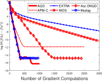
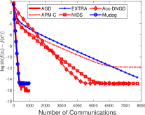
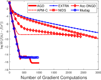
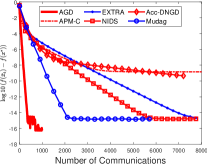
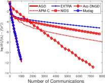
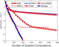
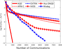
Figure 1: Comparisons with logistic regression and random networks. Each $f_{i}(x)$ is strongly convex ($\sigma_{i}=0.001$ in the top row, and $\sigma_{i}=0.0001$ in the bottom row). Random networks have $1-\lambda_{2}(W)=0.81$ in the left two columns and $1-\lambda_{2}(W)=0.05$ in the right two columns.

We compare our algorithm (Mudag) to centralized accelerated gradient descent (AGD) in (Nesterov, 2018), EXTRA in (Shi et al., 2015b), NIDS in (Li et al., 2019), Acc-DNGD in (Qu and Li, 2019) and APM-C in (Li et al., 2020b). In this paper, we do not compare our algorithm to the dual-based algorithms such as accelerated dual ascent algorithm (Uribe et al., 2020; Scaman et al., 2017) because these algorithms cannot be applied to the case where some functions $f_{i}(x)$ are non-convex. The step sizes of all algorithms are well-tuned to achieve their best performances. Furthermore, we set the momentum coefficient as ${\big{(}\sqrt{L}-\sqrt{\mu}\big{)}}/{\big{(}\sqrt{L}+\sqrt{\mu}\,\big{)}}$ for Mudag, AGD and APM-C. We initialize $\mathbf{x}_{0}$ at $\mathbf{0}$ for all the compared methods.

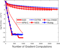
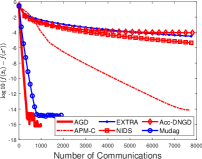
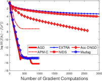
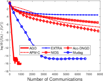
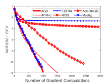
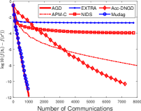
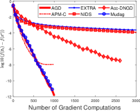
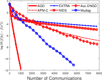
Figure 2: Comparisons with logistic regression and random networks. Each local objective $f_{i}(x)$ may be non-convex. In the top row, $\sigma_{i}=-10^{-2}$ for agents $i=1\dots,m-1$ and $\sigma_{i}=1$ for the agent $i=m$. In the bottom row, $\sigma_{i}=-10^{-1}$ for agents $i=1\dots,m-1$, and $\sigma_{i}=10$ for the agent $i=m$. Random networks have $1-\lambda_{2}(W)=0.81$ in the left two columns and $1-\lambda_{2}(W)=0.05$ in the right two columns.

In the setting in which each $f_{i}(x)$ is strongly convex, we report the experimental results in Figure 1. Compared with AGD, our algorithm has almost the same computation cost, which validates our theoretical analysis. Assuming that AGD communicates once per iteration, we can also see that the communication cost of Mudag is almost the same communication cost as that of AGD when $1-\lambda_{2}(W)=0.81$, and six times of that of AGD when $1-\lambda_{2}(W)=0.05$. This matches the theoretical results of communication complexity for our algorithm. Furthermore, our algorithm achieves both lower computation cost and lower communication cost than other decentralized algorithms on all settings. The advantages are more obvious for small $\sigma_{i}$, which also validates the comparison of the upper bounds with related works.

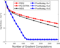
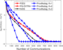
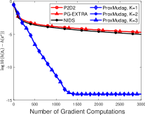
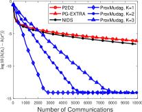
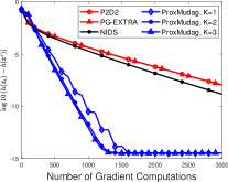
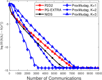
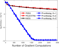
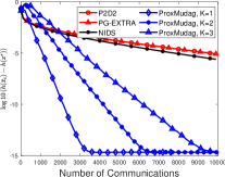
Figure 3: Comparisons with sparse logistic regression and random networks. In the top row, experiments on ‘a9a’ with $\sigma_{i}=10^{-3}$ for agents $i=1,\dots,m$ in the left two columns and $\sigma_{i}=10^{-4}$ in the right two columns. In the bottom row, experiments on ‘w8a’ with $\sigma_{i}=10^{-3}$ for agents $i=1,\dots,m$ in the left two columns and $\sigma_{i}=10^{-4}$ in the right two columns.

In the setting in which an individual function $f_{i}(x)$ could be non-convex, we report the experimental results in Figure 2. Note that the global objective function of experiments reported in Figure 1 and Figure 2 are the same but the model that corresponds to Figure 2 contains some non-convex $f_{i}(x)$. Comparing the curves in these two figures, we can observe that the computation cost of AGD and our algorithm are not affected by the non-convexity of $f_{i}(x)$ because their convergence rates only depend on $\sqrt{\kappa_{g}}$. On the other hand, the communication cost of our algorithm increases slightly compared to the setting where each $f_{i}(x)$ is convex. This is because the ratio $M/L$ of $f_{i}(x)$ increases when we set $\sigma_{i}=-10^{-1}$ or $\sigma_{i}=-10^{-2}$ for agent $i=1,\dots,m-1$. Our communication complexity theory shows $M/L$ will affect the communication cost by a $\log(M/L)$ factor. Compared with our algorithm, the performance of the other decentralized algorithms deteriorates greatly, which can be clearly observed by comparing the two figures in the top right corners of Figure 1 and Figure 2.

6.3 Experiments on Sparse Logistic Regression

We consider the sparse logistic regression model whose objective function is defined as

$$h(x)=\frac{1}{m}\sum_{i=1}^{m}f_{i}(x)+\gamma\left\|x\right\|_{1},$$

where $f_{i}(x)$ is defined in Eq. (31). We conduct experiments on the graph with $1-\lambda_{2}(W)=0.05$ and $f_{i}(x)$ and only consider the case when each $f_{i}(x)$ is convex, since experiments on logistic regression have already shown the advantage of our ideas for non-convex $f_{i}(x)$. We conduct experiments on the datasets ‘a9a’ and ‘w8a’, which can be downloaded from Libsvm datasets. For ‘w8a’, we set $n=497$ and $d=300$. For ‘a9a’, we set $n=325$ and $d=123$. We conduct the following two experimental settings:

1. We set $\gamma=10^{-4}$ and $\sigma_{1}=\dots=\sigma_{m}=10^{-3}$.

2. We set $\gamma=10^{-4}$ and $\sigma_{1}=\dots=\sigma_{m}=10^{-4}$.

We compare our algorithm (ProxMudag) with the state-of-the-art algorithms PG-EXTRA (Shi et al., 2015a), NIDS (Li et al., 2019) and decentralized proximal algorithm (D2P2) (Alghunaim et al., 2019). In the experiments, we set $K=1$, $K=2$ and $K=3$ in ProxMudag to evaluate how $K$ affects the convergence behavior. The parameters of all algorithms are well-tuned. We report the experimental results in Figure 3. We can observe that ProxMudag  outperforms other algorithms in all cases. First, ProxMudag  takes much less computation cost than other algorithms since ProxMudag  uses Nesterov’s acceleration to achieve a faster convergence rate. This matches our theoretical analysis of the computation complexity. We can further observe that the advantage of ProxMudag is more clear when $\sigma_{2}$ is small. This is because the small $\sigma_{i}$’s commonly lead to large condition numbers and the computation complexity of ProxMudag depends on $\sqrt{\kappa_{g}}$ instead of $\kappa_{\ell}$ or $\sqrt{\kappa_{\ell}}$. The results also show ProxMudag  has great advantages over other state-of-the-art decentralized proximal algorithms on the communication cost.

7 Conclusion

In this paper, we proposed two novel decentralized algorithms, which achieve the optimal computation complexity and the near optimal communication complexity. To the best of our knowledge, this is the best communication complexity that primal-based decentralized algorithms can achieve especially for the decentralized composite optimization problems.

Our results provide an affirmative answer to the open problem whether there is a decentralized algorithm that can achieve the communication complexity $\mathcal{O}\big{(}\sqrt{{\kappa_{g}}/{(1-\lambda_{2}(W))}}\log({1}/{\epsilon})\big{)}$ or even close to this lower bound for a strongly convex objective function. Furthermore, our algorithm does not require each individual functions $f_{i}(x)$ to be convex. Our experiments showed that the non-convexity of individual function $f_{i}(x)$ rarely degrades the performance of our algorithm. Our analysis also implies that integrating multi-consensus and gradient tracking can well approximate the decentralized optimization algorithm to the corresponding centralized counterpart. The implementation of the resulting algorithms are simple, effective and with (near) optimal complexities. This novel perspective may also provide useful insights for developing new decentralized optimization algorithms in other settings.

A Useful Lemmas

Lemma 12

For any matrix $\mathbf{x}\in\mathbb{R}^{m\times d}$ and $\bar{x}=\frac{1}{m}\mathbf{1}^{\top}\mathbf{x}$, it holds that

$$\left\|\mathbf{x}-\mathbf{1}\bar{x}\right\|^{2}\leq\left\|\mathbf{x}\right\|^{2}.$$ (32)

Proof  It holds that

$$\left\|\mathbf{x}-\mathbf{1}\bar{x}\right\|^{2}$$

$$= \sum_{j=1}^{m}\left\|\mathbf{x}(j,:)-\frac{1}{m}\sum_{i=1}^{m}\mathbf{x}(i,:)\right\|^{2}$$

$$= \sum_{j=1}^{m}\left(\left\|\mathbf{x}(j,:)\right\|^{2}-\frac{2}{m}\sum_{i=1}^{m}\left\langle\mathbf{x}(j,:),\mathbf{x}(i,:)\right\rangle+\frac{1}{m^{2}}\left\|\sum_{i=1}^{m}\mathbf{x}(i,:)\right\|^{2}\right)$$

$$= \left\|\mathbf{x}\right\|^{2}-\frac{2}{m}\sum_{i=1}^{m}\sum_{j=1}^{m}\left\langle\mathbf{x}(j,:),\mathbf{x}(i,:)\right\rangle+\frac{1}{m}\sum_{i=1}^{m}\sum_{j=1}^{m}\left\langle\mathbf{x}(j,:),\mathbf{x}(i,:)\right\rangle$$

$$\leq \left\|\mathbf{x}\right\|^{2}.$$

 

Lemma 13

We have

$$\left\|\nabla F(\mathbf{y})-\nabla F(\mathbf{x})\right\|\leq M\left\|\mathbf{y}-\mathbf{x}\right\|$$ (33)

and

$$\left\|\bar{g}_{t}-\nabla f(\bar{y}_{t})\right\|\leq\frac{M}{\sqrt{m}}\left\|\mathbf{y}_{t}-\mathbf{1}\bar{y}_{t}\right\|.$$ (34)

Furthermore, we have the $(L+2/\eta)$-smooth property for the generalized gradient $\tilde{\nabla}h(\cdot)$ (defined in Eq. (42)), i.e.,

$$\left\|\tilde{\nabla}h(x)-\tilde{\nabla}h(y)\right\|\leq\left(\frac{2}{\eta}+L\right)\left\|x-y\right\|.$$ (35)

Proof  The first inequality is because each $f_{i}(x)$ is $M$-smooth and

$$\left\|\nabla F(\mathbf{y})-\nabla F(\mathbf{x})\right\|= \sqrt{\sum_{i}^{m}\left\|\nabla f_{i}(\mathbf{y}(i,:))-\nabla f_{i}(\mathbf{x}(i,:))\right\|^{2}}$$

$$\leq \sqrt{M^{2}\sum_{i}^{m}\left\|\mathbf{y}(i,:)-\mathbf{x}(i,:)\right\|^{2}}=M\left\|\mathbf{y}-\mathbf{x}\right\|.$$

The second inequality follows from

$$\left\|\bar{g}_{t}-\nabla f(\bar{y}_{t})\right\|= \left\|\sum_{i=1}^{m}\frac{\nabla f_{i}(\mathbf{y}_{t}(i,:))-\nabla f_{i}(\bar{y}_{t})}{m}\right\|\leq M\sum_{i=0}^{m}\frac{\left\|\mathbf{y}_{t}(i,:)-\bar{y}_{t}\right\|}{m}$$

$$\leq M\sqrt{\sum_{i=1}^{m}\frac{\left\|\mathbf{y}_{t}(i,:)-\bar{y}_{t}\right\|^{2}}{m}}=\frac{M}{\sqrt{m}}\left\|\mathbf{y}_{t}-\mathbf{1}\bar{y}_{t}\right\|.$$

Then we can prove Eq. (35) using $L$-smoothness of $f(x)$ and the non-expansiveness of the proximal operator

$$\left\|\tilde{\nabla}h(x)-\tilde{\nabla}h(y)\right\|= \left\|\frac{x-{\rm{\bf prox}}_{\eta,r}(x-\eta\nabla f(x))}{\eta}-\frac{y-{\rm{\bf prox}}_{\eta,r}(y-\eta\nabla f(y))}{\eta}\right\|$$

$$\leq \frac{1}{\eta}\left\|x-y\right\|+\frac{1}{\eta}\left\|{\rm{\bf prox}}_{\eta,r}(x-\eta\nabla f(x))-{\rm{\bf prox}}_{\eta,r}(y-\eta\nabla f(y))\right\|$$

$$\leq \frac{1}{\eta}\left\|x-y\right\|+\frac{1}{\eta}\left\|(x-\eta\nabla f(x))-(y-\eta\nabla f(y))\right\|$$

$$\leq \left(\frac{2}{\eta}+L\right)\left\|x-y\right\|,$$

where the last inequality is due to the $L$-smoothness of $f(x)$.  

Lemma 14

For $\bar{x}_{t}$, $\bar{y}_{t}$ and $\bar{v}_{t}$ defined in Eqs. (3) and (18), then we can obtain that

$$\bar{y}_{t}-\bar{x}_{t} =\alpha(\bar{v}_{t}-\bar{y}_{t}),$$ (36)

$$\bar{y}_{t+1} =\frac{\bar{x}_{t+1}+\alpha\bar{v}_{t+1}}{1+\alpha},$$ (37)

and

$$\bar{v}_{t+1} =\begin{cases}(1-\alpha)\bar{v}_{t}+\alpha\bar{y}_{t}-\dfrac{\eta}{\alpha}\bar{G}_{t}\quad&r(x),\mbox{ is convex,}\\[8.5359pt] (1-\alpha)\bar{v}_{t}+\alpha\bar{y}_{t}-\dfrac{\eta}{\alpha}\bar{g}_{t},\quad&r(x)=0.\end{cases}$$ (38)

Proof  First using the definition of $\bar{v}_{t}$, we have

$$\frac{\bar{x}_{t+1}+\alpha\bar{v}_{t+1}}{1+\alpha}\stackrel{{\scriptstyle\eqref{eq:v_t}}}{{=}} \frac{\bar{x}_{t+1}+\alpha[\bar{x}_{t}+\frac{1}{\alpha}(\bar{x}_{t+1}-\bar{x}_{t})]}{1+\alpha}$$

$$= \bar{x}_{t+1}+\frac{1-\alpha}{1+\alpha}(\bar{x}_{t+1}-\bar{x}_{t})$$

$$= \bar{y}_{t+1}.$$

Then we can have

$$\bar{y}_{t}-\bar{x}_{t}=\alpha(\bar{v}_{t}-\bar{y}_{t}).$$

Now, we are going to prove Eq. (38) with the case $r(x)$ is convex since $r(x)=0$ is a special case of $r(x)$ being convex. Then we have

$$(1-\alpha)\bar{v}_{t}+\alpha\bar{y}_{t}-\frac{\eta}{\alpha}\bar{G}_{t}= \bar{v}_{t}-\alpha(\bar{v}_{t}-\bar{y}_{t})-\frac{\eta}{\alpha}\bar{G}_{t}=\bar{x}_{t}+\bar{v}_{t}-\bar{y}_{t}-\frac{\eta}{\alpha}\bar{G}_{t}$$

$$= \bar{x}_{t}+\frac{1}{\alpha}(\bar{y}_{t}-\bar{x}_{t}-\eta\bar{G}_{t})=\bar{x}_{t}+\frac{1}{\alpha}(\bar{x}_{t+1}-\bar{x}_{t})=\bar{v}_{t+1}.$$

 

Lemma 15

Let $f(x)$ be $\mu$-strongly convex. For $\bar{y}_{t}$, and $V_{t}$ defined in Eqs. (3) and (17) and $x^{*}$ being the optimum, we have the following inequality,

$$\left\|\bar{y}_{t}-x^{*}\right\|\leq\sqrt{\frac{2V_{t}}{\mu}}.$$ (39)

Proof  Since $f(x)$ is $\mu$-strongly convex, $h(x)$ in Eq. (1) is also $\mu$-strongly convex. Thus, we obtain

$$\left\|\bar{y}_{t}-x^{*}\right\|\stackrel{{\scriptstyle\eqref{eq:y_v}}}{{=}} \left\|\frac{\bar{x}_{t}+\alpha\bar{v}_{t}}{1+\alpha}-x^{*}\right\|\leq\frac{1}{1+\alpha}\left\|\bar{x}_{t}-x^{*}\right\|+\frac{\alpha}{1+\alpha}\left\|\bar{v}_{t}-x^{*}\right\|$$

$$\leq \frac{1}{1+\alpha}\sqrt{\frac{2(h(\bar{x})-h(x^{*}))}{\mu}}+\frac{\alpha}{1+\alpha}\sqrt{\frac{2}{\mu}\cdot\frac{\mu}{2}\left\|\bar{v}_{t}-x^{*}\right\|^{2}}\leq\sqrt{\frac{2V_{t}}{\mu}}.$$

 

At the end of this section, we provide the proof of Proposition 1.

Proof  We let

$$\Pi=I-\frac{1}{n}\mathbf{1}\mathbf{1}^{\top},\qquad\tilde{\Pi}=\begin{bmatrix}\Pi&0\\ 0&\Pi\end{bmatrix}\qquad\text{and}\qquad\tilde{W}=\begin{bmatrix}(1+\eta_{w})W&-\eta_{w}W\\ I&0\end{bmatrix},$$

then the iteration of Algorithm 2 can be written as

$$\begin{bmatrix}\mathbf{x}_{k+1}\\ \mathbf{x}_{k}\end{bmatrix}=\tilde{W}\begin{bmatrix}\mathbf{x}_{k}\\ \mathbf{x}_{k-1}\end{bmatrix}.$$

The property $W\mathbf{1}=\mathbf{1}$ directly leads to $\bar{x}=\frac{1}{m}\mathbf{1}^{\top}\mathbf{x}^{K}$. It also indicates

$$W\Pi=W\left(I-\frac{1}{n}\mathbf{1}\mathbf{1}^{\top}\right)=W-\frac{1}{n}W\mathbf{1}\mathbf{1}^{\top}=W-\frac{1}{n}\mathbf{1}\mathbf{1}^{\top}$$

and

$$\Pi W=\left(I-\frac{1}{n}\mathbf{1}\mathbf{1}^{\top}\right)W=W-\frac{1}{n}\mathbf{1}\mathbf{1}^{\top}W=W-\frac{1}{n}\mathbf{1}\mathbf{1}^{\top},$$

which means

$$\Pi W=W\Pi.$$ (40)

Consequently, we achieve

$$\tilde{W}\tilde{\Pi}= \begin{bmatrix}(1+\eta_{w})W&-\eta_{w}W\\ I&0\end{bmatrix}\begin{bmatrix}\Pi&0\\ 0&\Pi\end{bmatrix}$$

$$= \begin{bmatrix}(1+\eta_{w})W\Pi&-\eta_{w}W\Pi\\ \Pi&0\end{bmatrix},$$

$$\tilde{\Pi}\tilde{W}= \begin{bmatrix}\Pi&0\\ 0&\Pi\end{bmatrix}\begin{bmatrix}(1+\eta_{w})W&-\eta_{w}W\\ I&0\end{bmatrix}$$

$$= \begin{bmatrix}(1+\eta_{w})W\Pi&-\Pi\eta_{w}W\\ \Pi&0\end{bmatrix},$$

and

$$\tilde{\Pi}\tilde{W}\tilde{\Pi}= \begin{bmatrix}\Pi&0\\ 0&\Pi\end{bmatrix}\begin{bmatrix}(1+\eta_{w})W\Pi&-\eta_{w}W\Pi\\ \Pi&0\end{bmatrix}$$

$$= \begin{bmatrix}(1+\eta_{w})\Pi W\Pi&-\eta_{w}\Pi W\Pi\\ \Pi^{2}&0\end{bmatrix}$$

$$= \begin{bmatrix}(1+\eta_{w})\Pi W&-\eta_{w}\Pi W\\ \Pi&0\end{bmatrix}$$

$$= \tilde{\Pi}\tilde{W}=\tilde{W}\tilde{\Pi},$$

where we use the equality (40). This implies for any $K\geq 2$, we have

$$\tilde{\Pi}\tilde{W}^{K}=(\tilde{\Pi}\tilde{W})\tilde{W}^{K-1}=(\tilde{\Pi}\tilde{W}\tilde{\Pi})\tilde{W}^{K-1}=(\tilde{\Pi}\tilde{W})\tilde{\Pi}\tilde{W}^{K-1}$$

$$= (\tilde{\Pi}\tilde{W})^{2}\tilde{\Pi}\tilde{W}^{K-2}=\dots=(\tilde{\Pi}\tilde{W})^{K}\tilde{\Pi}$$

$$= \tilde{\Pi}(\tilde{W}\tilde{\Pi})^{K}=\tilde{\Pi}\tilde{W}(\tilde{\Pi}\tilde{W})^{K-1}\tilde{\Pi}$$

$$= \tilde{\Pi}\tilde{W}(\tilde{\Pi}\tilde{W})^{K-2}\tilde{\Pi}\tilde{W}\tilde{\Pi}$$

$$= \tilde{\Pi}\tilde{W}(\tilde{\Pi}\tilde{W})^{K-2}\tilde{W}\tilde{\Pi}=\dots=\tilde{\Pi}\tilde{W}\tilde{W}^{K-1}\tilde{\Pi}$$

$$= \tilde{\Pi}\tilde{W}^{K}\tilde{\Pi}.$$

Combining above result with Lemma 9 of Song et al. (2023), we have

$$\left\|\mathbf{x}_{K}-\mathbf{1}\bar{x}\right\|=\left\|\Pi\mathbf{x}_{K}\right\|$$

$$\leq \left\|\tilde{\Pi}\begin{bmatrix}\mathbf{x}_{K}\\ \mathbf{x}_{K-1}\end{bmatrix}\right\|=\left\|\tilde{\Pi}\tilde{W}^{K}\begin{bmatrix}\mathbf{x}_{0}\\ \mathbf{x}_{-1}\end{bmatrix}\right\|=\left\|\tilde{\Pi}\tilde{W}^{K}\tilde{\Pi}\begin{bmatrix}\mathbf{x}_{0}\\ \mathbf{x}_{-1}\end{bmatrix}\right\|$$

$$\leq \sqrt{14}\tilde{\rho}_{w}^{K}\left\|\Pi\mathbf{x}_{0}\right\|=\sqrt{14}\tilde{\rho}_{w}^{K}\left\|\mathbf{x}_{0}-\mathbf{1}\bar{x}\right\|,$$

where

$$\tilde{\rho}_{w}=\frac{1}{\sqrt{1+\sqrt{1-\lambda_{2}^{2}(W)}}}.$$

Since we have

$$\frac{1}{\sqrt{1+x}}\leq 1-\left(1-\frac{1}{\sqrt{2}}\right)x,$$ (41)

for any $x\in[0,1]$, it holds that

$$\tilde{\rho}_{w}= \frac{1}{\sqrt{1+\sqrt{1-\lambda_{2}^{2}(W)}}}$$

$$\leq 1-\left(1-\frac{1}{\sqrt{2}}\right)\sqrt{1-\lambda_{2}^{2}(W)}$$

$$\leq 1-\left(1-\frac{1}{\sqrt{2}}\right)\sqrt{1-\lambda_{2}(W)}.$$

This implies

$$\left\|\mathbf{x}_{K}-\mathbf{1}\bar{x}\right\|\leq\sqrt{14}\left(1-\left(1-\frac{1}{\sqrt{2}}\,\right)\sqrt{1-\lambda_{2}(W)}\right)^{K}\left\|\mathbf{x}_{0}-\mathbf{1}\bar{x}\right\|.$$

 

B Proof of Lemmas in Section 5

B.1 Collection of Lemmas

We list several important lemmas that will be used in our proofs.

Lemma 16 (Nesterov (2018))

Letting $\tilde{\nabla}h(x)$ the generalized gradient of $h(x)$ (refer to Eq. (1)) be defined as

$$\tilde{\nabla}h(x)\triangleq\frac{x-{\rm{\bf prox}}_{\eta,r}(x-\eta\nabla f(x))}{\eta},\;\mbox{with}\;\eta\;\mbox{being the step size},$$ (42)

then it holds that $\tilde{\nabla}h(x^{*})=0$ if $x^{*}$ minimizes $h(x)$.

Lemma 17

Letting ${\rm{\bf prox}}_{\eta m,R}^{(i)}(\mathbf{x})$ denote the $i$-th row of the matrix ${\rm{\bf prox}}_{\eta m,R}(\mathbf{x})$ (defined in Eqn. (4)), we have the following equation

$${\rm{\bf prox}}_{\eta m,R}^{(i)}(\mathbf{x})={\rm{\bf prox}}_{\eta,r}(\mathbf{x}^{(i)}),$$

which implies that $G_{t}^{(i)}$ equals to the $i$-th row of $G_{t}$ defined in Eq. (5).

Proof  By the definition of the proximal operators, we have

$${\rm{\bf prox}}_{\eta m,R}(\mathbf{x})= \mathop{\mathrm{argmin}}_{\mathbf{z}}\left(R(\mathbf{z})+\frac{1}{2\eta m}\left\|\mathbf{z}-\mathbf{x}\right\|_{F}^{2}\right)$$

$$= \mathop{\mathrm{argmin}}_{\mathbf{z}}\left(\frac{1}{m}\sum_{i=1}^{m}r(\mathbf{z}^{(i)})+\sum_{i=1}^{m}\frac{1}{2\eta m}\left\|\mathbf{z}^{(i)}-\mathbf{x}^{(i)}\right\|^{2}\right)$$

$$= \mathop{\mathrm{argmin}}_{\mathbf{z}}\left(\sum_{i=1}^{m}r(\mathbf{z}^{(i)})+\sum_{i=1}^{m}\frac{1}{2\eta}\left\|\mathbf{z}^{(i)}-\mathbf{x}^{(i)}\right\|^{2}\right)$$

$$= \begin{pmatrix}\mathop{\mathrm{argmin}}_{z}\left(r(z)+\frac{1}{2\eta}\left\|z-\mathbf{x}^{(1)}\right\|\right)^{\top}\\ \vdots\\ \mathop{\mathrm{argmin}}_{z}\left(r(z)+\frac{1}{2\eta}\left\|z-\mathbf{x}^{(m)}\right\|\right)^{\top}\end{pmatrix}.$$

Therefore, we have the following equation

$${\rm{\bf prox}}_{\eta m,R}^{(i)}(\mathbf{x})={\rm{\bf prox}}_{\eta,r}(\mathbf{x}^{(i)}).$$

 

Lemma 18

For any $\mathbf{x}\in\mathbb{R}^{m\times d}$, ${\rm{\bf prox}}_{m\eta,R}(\cdot)$ (defined in Eq. (4)) has the following property

$$\left\|{\rm{\bf prox}}_{\eta m,R}\left(\frac{1}{m}\mathbf{1}\mathbf{1}^{\top}\mathbf{x}\right)-\frac{1}{m}\mathbf{1}\mathbf{1}^{\top}{\rm{\bf prox}}_{\eta m,R}(\mathbf{x})\right\|\leq\left\|\mathbf{x}-\mathbf{1}\bar{x}_{t}\right\|.$$ (43)

Proof  Using Lemma 17 and non-expansiveness of the proximal mapping, we have

$$\left\|{\rm{\bf prox}}_{\eta m,R}(\frac{1}{m}\mathbf{1}\mathbf{1}^{\top}\mathbf{x})-\frac{1}{m}\mathbf{1}\mathbf{1}^{\top}{\rm{\bf prox}}_{\eta m,R}(\mathbf{x})\right\|^{2}$$

$$= {m\left\|{\rm{\bf prox}}_{\eta,r}(\frac{1}{m}\mathbf{1}^{\top}\mathbf{x})-\frac{1}{m}\sum_{i=1}^{m}{\rm{\bf prox}}_{\eta,r}(\mathbf{x}^{(i)})\right\|^{2}}$$

$$= m\left\|\frac{1}{m}\sum_{i=1}^{m}\left({\rm{\bf prox}}_{\eta,r}(\frac{1}{m}\mathbf{1}^{\top}\mathbf{x})-{\rm{\bf prox}}_{\eta,r}(\mathbf{x}^{(i)})\right)\right\|^{2}$$

$$\leq \sum_{i=1}^{m}\left\|\left({\rm{\bf prox}}_{\eta,r}(\frac{1}{m}\mathbf{1}^{\top}\mathbf{x})-{\rm{\bf prox}}_{\eta,r}(\mathbf{x}^{(i)})\right)\right\|^{2}$$

$$\leq {\sum_{i=1}^{m}\left\|\left(\frac{1}{m}\mathbf{1}^{\top}\mathbf{x}-\mathbf{x}^{(i)}\right)\right\|^{2}}=\left\|\mathbf{x}-\mathbf{1}\bar{x}_{t}\right\|^{2}.$$

 

Lemma 19

Letting $\mathbf{s}_{t}^{(i)}$ be the $i$-th row of $\mathbf{s}_{t}$ and $G_{t}^{(i)},\;\bar{G}_{t}$ (defined in Eqs. (5), (6)) generated by Algorithm 3, we have

$$\sum_{i=1}^{m}\left\|\mathbf{s}_{t}^{(i)}-\nabla f(\mathbf{y}_{t}^{(i)})\right\|^{2}\leq 2\left\|\mathbf{s}_{t}-\mathbf{1}\bar{s}_{t}\right\|^{2}+8M^{2}\left\|\mathbf{y}_{t}-\mathbf{1}\bar{y}_{t}\right\|^{2}$$ (44)

and

$$\eta^{2}\sum_{i=1}^{m}\left\|G_{t}^{(i)}-\bar{G}_{t}\right\|^{2}\leq 18\left\|\mathbf{y}_{t}-\mathbf{1}\bar{y}_{t}\right\|^{2}+16\eta^{2}\left\|\mathbf{s}_{t}-\mathbf{1}\bar{s}_{t}\right\|^{2}.$$ (45)

Proof  Using the inequality that $(a+b)^{2}\leq 2a^{2}+2b^{2}$, we have

$$\sum_{i=1}^{m}\left\|\mathbf{s}_{t}^{(i)}-\nabla f(\mathbf{y}_{t}^{(i)})\right\|^{2}\leq 2\sum_{i=1}^{m}\left\|\mathbf{s}_{t}^{(i)}-\bar{s}_{t}\right\|^{2}+2\sum_{i=1}^{m}\left\|\bar{s}_{t}-\nabla f(\mathbf{y}_{t}^{(i)})\right\|^{2}$$

$$\leq 2\sum_{i=1}^{m}\left\|\mathbf{s}_{t}^{(i)}-\bar{s}_{t}\right\|^{2}+4\sum_{i=1}^{m}\left\|\bar{s}_{t}-\nabla f(\bar{y}_{t})\right\|^{2}+4\sum_{i=1}^{m}\left\|\nabla f(\bar{y}_{t})-\nabla f(\mathbf{y}_{t}^{(i)})\right\|^{2}$$

$$\leq 2\left\|\mathbf{s}_{t}-\mathbf{1}\bar{s}_{t}\right\|^{2}+4M^{2}\left\|\mathbf{1}\bar{y}_{t}-\mathbf{y}_{t}\right\|^{2}+4L^{2}\left\|\mathbf{1}\bar{y}_{t}-\mathbf{y}_{t}\right\|^{2}$$

$$\leq 2\left\|\mathbf{s}_{t}-\mathbf{1}\bar{s}_{t}\right\|^{2}+8M^{2}\left\|\mathbf{1}\bar{y}_{t}-\mathbf{y}_{t}\right\|^{2},$$

where the third inequality is from Eq. (34) and the $L$-smoothness of $f(x)$, the last inequality is due to $L\leq M$.

Furthermore, it holds that

$$\small\begin{split}&\eta^{2}\sum_{i=1}^{m}\left\|G_{t}^{(i)}-\bar{G}_{t}\right\|^{2}=\left\|\eta G_{t}-\frac{\eta}{m}\mathbf{1}\cdot\mathbf{1}^{\top}G_{t}\right\|^{2}\\ =&\sum_{i=1}^{m}\left\|\mathbf{y}_{t}^{(i)}-{\rm{\bf prox}}_{\eta,r}(\mathbf{y}_{t}^{(i)}-\eta\mathbf{s}_{t}^{(i)})-\frac{1}{m}\sum_{j=1}^{m}\left(\mathbf{y}_{t}^{(j)}-{\rm{\bf prox}}_{\eta,r}(\mathbf{y}_{t}^{(j)}-\eta\mathbf{s}_{t}^{(j)})\right)\right\|^{2}\\ \leq&2\sum_{i=1}^{m}\left\|\mathbf{y}_{t}^{(i)}-\bar{y}_{t}\right\|^{2}+2\sum_{i=1}^{m}\left\|{\rm{\bf prox}}_{\eta,r}(\mathbf{y}_{t}^{(i)}-\eta\mathbf{s}_{t}^{(i)})-\frac{1}{m}\sum_{j=1}^{m}{\rm{\bf prox}}_{\eta,r}(\mathbf{y}_{t}^{(j)}-\eta\mathbf{s}_{t}^{(j)})\right\|^{2}\\ \leq&2\sum_{i=1}^{m}\left\|\mathbf{y}_{t}^{(i)}-\bar{y}_{t}\right\|^{2}+4\sum_{i=1}^{m}\left\|{\rm{\bf prox}}_{\eta,r}(\mathbf{y}_{t}^{(i)}-\eta\mathbf{s}_{t}^{(i)})-{\rm{\bf prox}}_{\eta,r}(\bar{y}_{t}-\eta\bar{s}_{t})\right\|^{2}\\ &+4\sum_{i=1}^{m}\left\|{\rm{\bf prox}}_{\eta,r}(\bar{y}_{t}-\eta\bar{s}_{t})-\frac{1}{m}\sum_{j=1}^{m}{\rm{\bf prox}}_{\eta,r}(\mathbf{y}_{t}^{(j)}-\eta\mathbf{s}_{t}^{(j)})\right\|^{2}\\ \leq&2\left\|\mathbf{y}_{t}-\mathbf{1}\bar{y}_{t}\right\|^{2}+4\sum_{i=1}^{m}\left\|\mathbf{y}_{t}^{(i)}-\bar{y}_{t}-\eta(\mathbf{s}_{t}^{(i)}-\bar{s}_{t})\right\|^{2}+4\sum_{i=1}^{m}\left\|{\rm{\bf prox}}_{\eta,r}(\bar{y}_{t}-\eta\bar{s}_{t})-{\rm{\bf prox}}_{\eta,r}(\mathbf{y}_{t}^{(i)}-\eta\mathbf{s}_{t}^{(i)})\right\|^{2}\\ \leq&2\left\|\mathbf{y}_{t}-\mathbf{1}\bar{y}_{t}\right\|^{2}+16\left\|\mathbf{y}_{t}-\mathbf{1}\bar{y}_{t}\right\|^{2}+16\eta^{2}\left\|\mathbf{s}_{t}-\mathbf{1}\bar{s}_{t}\right\|^{2}\\ =&18\left\|\mathbf{y}_{t}-\mathbf{1}\bar{y}_{t}\right\|^{2}+16\eta^{2}\left\|\mathbf{s}_{t}-\mathbf{1}\bar{s}_{t}\right\|^{2},\end{split}$$

where the third and forth inequalities are due to the non-expansiveness of proximal mapping.  

Lemma 20

Letting $\tilde{\nabla}h(\bar{y}_{t})$ be defined in Eq. (42), then we have the following error bound for the estimated generalized gradient

$$\eta\left\|\bar{G}_{t}-\tilde{\nabla}h(\bar{y}_{t})\right\|\leq \frac{4+2M\eta}{\sqrt{m}}\left\|\mathbf{y}_{t}-\mathbf{1}\bar{y}_{t}\right\|+\frac{2\eta}{\sqrt{m}}\left\|\mathbf{s}_{t}-\mathbf{1}\bar{s}_{t}\right\|.$$ (46)

Proof  It holds that

$$\eta\left\|\bar{G}_{t}-\eta\tilde{\nabla}h(\bar{y}_{t})\right\|=\sqrt{\left\|\frac{1}{m}\sum_{i=1}^{m}\left(\eta G_{t}^{(i)}-\eta\tilde{\nabla}h(\bar{y}_{t})\right)\right\|^{2}}\leq\sqrt{\frac{1}{m}\cdot\sum_{i=1}^{m}\left\|\left(\eta G_{t}^{(i)}-\eta\tilde{\nabla}h(\bar{y}_{t})\right)\right\|^{2}}$$

$$= \sqrt{\frac{1}{m}}\cdot\sqrt{\sum_{i=1}^{m}\left\|\left(\mathbf{y}_{t}^{(i)}-{\rm{\bf prox}}_{\eta,r}(\mathbf{y}_{t}^{(i)}-\eta\mathbf{s}_{t}^{(i)})\right)-\left(\bar{y}_{t}-{\rm{\bf prox}}_{\eta,r}(\bar{y}_{t}-\eta\nabla f(\bar{y}_{t}))\right)\right\|^{2}}$$

$$\leq \sqrt{\frac{1}{m}}\cdot\sqrt{\sum_{i=1}^{m}\left(2\left\|\mathbf{y}_{t}^{(i)}-\bar{y}_{t}\right\|^{2}+2\left\|{\rm{\bf prox}}_{\eta,r}(\mathbf{y}_{t}^{(i)}-\eta\mathbf{s}_{t}^{(i)})-{\rm{\bf prox}}_{\eta,r}(\bar{y}_{t}-\eta\nabla f(\bar{y}_{t}))\right\|^{2}\right)}$$

$$\leq \sqrt{\frac{1}{m}}\cdot\sqrt{\sum_{i=1}^{m}\left(2\left\|\mathbf{y}_{t}^{(i)}-\bar{y}_{t}\right\|^{2}+2\left\|(\mathbf{y}_{t}^{(i)}-\eta\mathbf{s}_{t}^{(i)})-(\bar{y}_{t}-\eta\nabla f(\bar{y}_{t}))\right\|^{2}\right)}$$

$$= \sqrt{\frac{1}{m}}\cdot\sqrt{2\left\|\mathbf{y}_{t}-\mathbf{1}\bar{y}_{t}\right\|^{2}+2\left\|\eta\mathbf{s}_{t}-\eta\mathbf{1}\nabla f(\bar{y}_{t})+\mathbf{y}_{t}-\mathbf{1}\bar{y}_{t}\right\|^{2}}$$

$$\leq \sqrt{\frac{1}{m}}\cdot\left(4\left\|\mathbf{y}_{t}-\mathbf{1}\bar{y}_{t}\right\|+2\eta\left\|\mathbf{s}_{t}-\mathbf{1}\bar{s}_{t}\right\|+2\eta\left\|\mathbf{1}\bar{s}_{t}-\mathbf{1}\nabla f(\bar{y}_{t})\right\|\right)$$

$$\leq \sqrt{\frac{1}{m}}\cdot\Big{(}(4+2M\eta)\left\|\mathbf{y}_{t}-\mathbf{1}\bar{y}_{t}\right\|+2\eta\left\|\bar{s}_{t}-\mathbf{1}\bar{s}_{t}\right\|\Big{)},$$

where the second inequality is due to the non-expansiveness of proximal operator, and the last inequality is from Eq. (34).

 

B.2 Proof of Lemma 9

Proof  For simplicity, we denote FastMix$(\cdot,K)$ operation as $\mathbb{T}(\cdot)$. From Proposition 1 we can know that

$$\left\|\mathbb{T}(\mathbf{x})-\frac{1}{m}\mathbf{1}\mathbf{1}^{\top}\mathbf{x}\right\|\leq\rho\left\|\mathbf{x}-\frac{1}{m}\mathbf{1}\mathbf{1}^{\top}\mathbf{x}\right\|.$$

First, we have

$$\left\|\mathbf{1}\bar{x}_{t+1}-\mathbf{x}_{t+1}\right\|$$ (47)

$$\leq \left\|{\rm{\bf prox}}_{\eta m,R}(\mathbf{y}_{t}-\eta\mathbf{s}_{t})-\frac{1}{m}\mathbf{1}\mathbf{1}^{\top}{\rm{\bf prox}}_{\eta m,R}(\mathbf{y}_{t}-\eta\mathbf{s}_{t})\right\|$$

$$\leq \left\|{\rm{\bf prox}}_{\eta m,R}(\mathbf{y}_{t}-\eta\mathbf{s}_{t})-{\rm{\bf prox}}_{\eta m,R}\left(\mathbf{1}(\bar{y}_{t}-\eta\bar{s}_{t})\right)\right\|$$

$$+\left\|{\rm{\bf prox}}_{\eta m,R}\left(\mathbf{1}(\bar{y}_{t}-\eta\bar{s}_{t})\right)-\frac{1}{m}\mathbf{1}\mathbf{1}^{\top}{\rm{\bf prox}}_{\eta m,R}(\mathbf{y}_{t}-\eta\mathbf{s}_{t})\right\|$$

$$\leq \left\|\mathbf{y}_{t}-\mathbf{1}\bar{y}_{t}\right\|+\eta\left\|\mathbf{s}_{t}-\mathbf{1}\bar{s}_{t}\right\|+\left\|\left(\mathbf{y}_{t}-\eta\mathbf{s}_{t}\right)-\mathbf{1}\left(\bar{y}_{t}-\eta\bar{s}_{t}\right)\right\|$$

$$\leq 2\left\|\mathbf{y}_{t}-\mathbf{1}\bar{y}_{t}\right\|+2\eta\left\|\mathbf{s}_{t}-\mathbf{1}\bar{s}_{t}\right\|,$$

where the third inequality is because of Lemma 18 and the non-expansiveness of proximal operator.

Using the definition of $\mathbf{y}_{t+1}$ in Algorithm 1 and the property of “FastMix” operation, we have

$$\left\|\mathbf{y}_{t+1}-\mathbf{1}\bar{y}_{t+1}\right\|$$ (48)

$$\leq \frac{2\rho}{1+\alpha}\left\|\mathbf{x}_{t+1}-\mathbf{1}\bar{x}_{t+1}\right\|+\rho\frac{1-\alpha}{1+\alpha}\left\|\mathbf{x}_{t}-\mathbf{1}\bar{x}_{t}\right\|$$

$$\stackrel{{\scriptstyle\eqref{eq:x_error}}}{{\leq}} 4\rho\left\|\mathbf{y}_{t}-\mathbf{1}\bar{y}_{t}\right\|+4\rho\eta\left\|\mathbf{s}_{t}-\mathbf{1}\bar{s}_{t}\right\|+\rho\left\|\mathbf{x}_{t}-\mathbf{1}\bar{x}_{t}\right\|.$$

Now we are going to bound the value of $\left\|\mathbf{s}_{t+1}-\mathbf{1}\bar{s}_{t+1}\right\|$. We have

$$\left\|\mathbf{s}_{t+1}-\mathbf{1}\bar{s}_{t+1}\right\|$$

$$\leq \rho\left\|\mathbf{s}_{t}+\nabla F(\mathbf{y}_{t+1})-\nabla F(\mathbf{y}_{t})-\mathbf{1}\cdot\left(\bar{s}_{t}+\bar{g}_{t+1}-\bar{g}_{t}\right)\right\|$$

$$\stackrel{{\scriptstyle\eqref{eq:xx_m}}}{{\leq}} \rho\left\|\mathbf{s}_{t}-\mathbf{1}\bar{s}_{t}\right\|+\rho M\left\|\mathbf{y}_{t+1}-\mathbf{y}_{t}\right\|$$

$$\leq \rho\left\|\mathbf{s}_{t}-\mathbf{1}\bar{s}_{t}\right\|+\rho M\left\|\mathbf{y}_{t+1}-\mathbf{1}\bar{y}_{t+1}\right\|+\rho M\left\|\mathbf{1}\bar{y}_{t+1}-\mathbf{1}\bar{y}_{t}\right\|+\rho M\left\|\mathbf{1}\bar{y}_{t}-\mathbf{y}_{t}\right\|$$

$$\stackrel{{\scriptstyle\eqref{eq:y_err}}}{{\leq}} \rho\left\|\mathbf{s}_{t}-\mathbf{1}\bar{s}_{t}\right\|+\rho M\left(4\rho\left\|\mathbf{y}_{t}-\mathbf{1}\bar{y}_{t}\right\|+4\rho\eta\left\|\mathbf{s}_{t}-\mathbf{1}\bar{s}_{t}\right\|+\rho\left\|\mathbf{x}_{t}-\mathbf{1}\bar{x}_{t}\right\|\right)$$

$$+\rho M\left\|\mathbf{1}\bar{y}_{t+1}-\mathbf{1}\bar{y}_{t}\right\|+\rho M\left\|\mathbf{1}\bar{y}_{t}-\mathbf{y}_{t}\right\|$$

$$= \left(\rho+4\rho^{2}M\eta\right)\left\|\mathbf{s}_{t}-\mathbf{1}\bar{s}_{t}\right\|+\rho^{2}M\left\|\mathbf{x}_{t}-\mathbf{1}\bar{x}_{t}\right\|+\left(\rho M+4\rho^{2}M\right)\left\|\mathbf{1}\bar{y}_{t}-\mathbf{y}_{t}\right\|+\rho M\left\|\mathbf{1}\bar{y}_{t+1}-\mathbf{1}\bar{y}_{t}\right\|$$

$$\leq \rho(1+4M\eta)\left\|\mathbf{s}_{t}-\mathbf{1}\bar{s}_{t}\right\|+\rho M\left\|\mathbf{x}_{t}-\mathbf{1}\bar{x}_{t}\right\|+5\rho M\left\|\mathbf{y}_{t}-\mathbf{1}\bar{y}_{t}\right\|+\rho M\left\|\mathbf{1}\bar{y}_{t+1}-\mathbf{1}\bar{y}_{t}\right\|,$$

where the last inequality is because of $\rho\leq 1$. Then we only need to consider the term $\left\|\mathbf{1}\bar{y}_{t+1}-\mathbf{1}\bar{y}_{t}\right\|$. Using the iteration of average variables illustrated in Eq. (20), we have

$$\left\|\bar{y}_{t+1}-\bar{y}_{t}\right\|$$

$$= \left\|\frac{2}{1+\alpha}\bar{x}_{t+1}-\frac{1-\alpha}{1+\alpha}\bar{x}_{t}-\bar{y}_{t}\right\|$$

$$= \left\|\frac{2}{1+\alpha}(\bar{y}_{t}-\eta\bar{G}_{t})-\frac{1-\alpha}{1+\alpha}\bar{x}_{t}-\bar{y}_{t}\right\|$$

$$\leq \frac{1-\alpha}{1+\alpha}\left\|\bar{y}_{t}-\bar{x}_{t}\right\|+\frac{2\eta}{1+\alpha}\left\|\bar{G}_{t}\right\|$$

$$\leq \left\|\bar{y}_{t}-x^{*}\right\|+\left\|\bar{x}_{t}-x^{*}\right\|+2\eta\left\|\bar{G}_{t}-\tilde{\nabla}h(\bar{y}_{t})\right\|+2\eta\left\|\tilde{\nabla}h(\bar{y}_{t})\right\|$$

$$\stackrel{{\scriptstyle\eqref{eq:G_h}}}{{\leq}} \left\|\bar{y}_{t}-x^{*}\right\|+\left\|\bar{x}_{t}-x^{*}\right\|+\frac{8+4M\eta}{\sqrt{m}}\left\|\mathbf{y}_{t}-\mathbf{1}\bar{y}_{t}\right\|+\frac{4\eta}{\sqrt{m}}\left\|\mathbf{s}_{t}-\mathbf{1}\bar{s}_{t}\right\|+2\eta\left\|\tilde{\nabla}h(\bar{y}_{t})\right\|.$$

Furthermore, by Lemma 15 and the fact that $\tilde{\nabla}h(x^{*})=0$, we can obtain

$$\small\begin{split}&2\eta\left\|\tilde{\nabla}h(\bar{y}_{t})\right\|+\left\|\bar{x}_{t}-x^{*}\right\|+\left\|\bar{y}_{t}-x^{*}\right\|\\ =&2\eta\left\|\tilde{\nabla}h(\bar{y}_{t})-\tilde{\nabla}h(x^{*})\right\|+\left\|\bar{x}_{t}-x^{*}\right\|+\left\|\bar{y}_{t}-x^{*}\right\|\\ =&2\left\|\bar{y}_{t}-{\rm{\bf prox}}_{\eta,r}(\bar{y}_{t}-\eta\nabla f(\bar{y}_{t}))-(x^{*}-{\rm{\bf prox}}_{\eta,r}(x^{*}-\eta\nabla f(x^{*})))\right\|+\left\|\bar{x}_{t}-x^{*}\right\|+\left\|\bar{y}_{t}-x^{*}\right\|\\ \stackrel{{\scriptstyle\eqref{eq:62}}}{{\leq}}&2\left\|\bar{y}_{t}-x^{*}\right\|+2\left\|\bar{y}_{t}-x^{*}\right\|+2\eta\left\|\nabla f(\bar{y}_{t})-\nabla f(x^{*})\right\|+\left\|\bar{x}_{t}-x^{*}\right\|+\left\|\bar{y}_{t}-x^{*}\right\|\\ \leq&(5+2\eta L)\left\|\bar{y}_{t}-x^{*}\right\|+\left\|\bar{x}_{t}-x^{*}\right\|\\ \stackrel{{\scriptstyle\eqref{eq:y_x_V}}}{{\leq}}&(5+2\eta L)\sqrt{\frac{2V_{t}}{\mu}}+\sqrt{\frac{2}{\mu}(h(\bar{x}_{t})-h(x^{*}))}\\ \leq&7\sqrt{\frac{2V_{t}}{\mu}},\end{split}$$

where the last equality is because of $\eta={1}/{(2L)}$. Thus, we can obtain that

$$\left\|\mathbf{1}\bar{y}_{t+1}-\mathbf{1}\bar{y}_{t}\right\|\leq(8+4M\eta)\left\|\mathbf{y}_{t}-\mathbf{1}\bar{y}_{t}\right\|+4\eta\left\|\mathbf{s}_{t}-\mathbf{1}\bar{s}_{t}\right\|+7\sqrt{m}\sqrt{\frac{2}{\mu}V_{t}}.$$

Combining above results, we can bound the value of $\eta\left\|\mathbf{s}_{t+1}-\mathbf{1}\bar{s}_{t+1}\right\|$ as follows

$$\eta\left\|\mathbf{s}_{t+1}-\mathbf{1}\bar{s}_{t+1}\right\|\leq \rho\left(1+8M\eta\right)\cdot\eta\left\|\mathbf{s}_{t}-\mathbf{1}\bar{s}_{t}\right\|+\rho\cdot M\eta\left\|\mathbf{x}_{t}-\mathbf{1}\bar{x}_{t}\right\|$$ (49)

$$+\rho M\eta\left(13+4M\eta\right)\left\|\mathbf{y}_{t}-\mathbf{1}\bar{y}_{t}\right\|+7\rho M\eta\sqrt{m}\sqrt{\frac{2}{\mu}V_{t}}$$

$$\leq \frac{5\rho M}{L}\cdot\eta\left\|\mathbf{s}_{t}-\mathbf{1}\bar{s}_{t}\right\|+\frac{\rho M}{L}\left\|\mathbf{x}_{t}-\mathbf{1}\bar{x}_{t}\right\|$$

$$+\frac{8\rho M^{2}}{L^{2}}\left\|\mathbf{y}_{t}-\mathbf{1}\bar{y}_{t}\right\|+\frac{4\rho M}{L}\sqrt{m}\sqrt{\frac{2}{\mu}V_{t}},$$

where the last inequality is because of $\eta={1}/{(2L)}$ and $1\leq{M}/{L}$.

Combining Eqs. (47), (48) and (49), we can obtain

$$\mathbf{z}_{t+1}\leq\mathbf{A}\mathbf{z}_{t}+\frac{4\rho M\sqrt{m}}{L}\left[0,0,\sqrt{\frac{2V_{t}}{\mu}}\,\right]^{\top},$$

where

$$\mathbf{A}=\begin{bmatrix}0&2&2\\ 2\rho&4\rho&4\rho\\ \rho M/L&8\rho M^{2}/L^{2}&5\rho M/L\end{bmatrix}.$$

 

B.3 Proof of Lemma 10

Proof  It is easy to check that $\mathbf{A}$ is non-negative and irreducible. Furthermore, every diagonal entry of $\mathbf{A}$ is not zero. Thus, by Perron-Frobenius theorem and Corollary 8.4.7 of Horn and Johnson (2012), $\mathbf{A}$ has a real-valued positive number $\lambda_{1}(\mathbf{A})$ which is algebraically simple and associated with a strictly positive eigenvector $\mathbf{v}$. It also holds that $\lambda_{1}(\mathbf{A})$ is strictly larger than $|\lambda_{i}(\mathbf{A})|$ with $i=2,3$.

We write down the characteristic polynomial $p(\zeta)$ of ${\mathbf{A}}$, that is

$$p(\zeta)=\zeta p_{0}(\zeta)-32(M/L)^{2}\rho^{2}+20\rho^{2}M/L,$$

where

$$p_{0}(\zeta)=\zeta^{2}-\rho\left(4+5M/L\right)\zeta-4\rho\left(8\rho(M/L)^{2}+5M/L+1-5\rho M/L\right).$$

Let us denote

$$\Delta=16\rho\left(8\rho(M/L)^{2}+5M/L+1-5\rho M/L\right).$$ (50)

It is easy to check that $\Delta>0$. Thus, two roots of $p_{0}(\zeta)$ are

$$\zeta_{1}=\frac{\rho(4+5M/L)+\sqrt{(4+5M/L)^{2}\rho^{2}+\Delta}}{2}$$

and

$$\zeta_{2}=\frac{\rho(4+5M/L)-\sqrt{(4+5M/L)^{2}\rho^{2}+\Delta}}{2}.$$

By letting

$$\zeta^{*}=\frac{2\rho\cdot\left(32(M/L)^{2}+2\right)(4+5M/L)+\sqrt{\max\{\Delta,\frac{1}{4}\}}}{2},$$

we have

$$p\left(\zeta^{*}\right)+32(M/L)^{2}\rho^{2}-20\rho^{2}M/L$$

$$= \frac{2\rho\left(32(M/L)^{2}+2\right)(4+5M/L)+\sqrt{\max\{\Delta,\frac{1}{4}\}}}{2}$$

$$\cdot\frac{2\rho\!\left(32(M/L)^{2}\!+\!2\right)(4\!+\!5M/L)+\sqrt{\max\{\Delta,\frac{1}{4}\}}-\rho(4\!+\!5M/L)-\sqrt{(4\!+\!5M/L)^{2}\rho^{2}\!+\!\Delta}}{2}$$

$$\cdot\frac{2\rho\!\left(32(M/L)^{2}\!+\!2\right)(4\!+\!5M/L)+\sqrt{\max\{\Delta,\frac{1}{4}\}}-\rho(4\!+\!5M/L)+\sqrt{(4\!+\!5M/L)^{2}\rho^{2}\!+\!\Delta}}{2}$$

$$\geq\frac{2\rho\left(32(M/L)^{2}+2\right)(4+5M/L)+\sqrt{\max\{\Delta,\frac{1}{4}\}}}{2}$$

$$\cdot\frac{\left(2\rho\left(32(M/L)^{2}+1\right)(4+5M/L)+\sqrt{\max\{\Delta,\frac{1}{4}\}}\,\right)^{2}-(\sqrt{(4+5M/L)^{2}\rho^{2}+\Delta})^{2}}{2}$$

$$= \frac{2\rho\left(32(M/L)^{2}+2\right)(4+5M/L)+\sqrt{\max\{\Delta,\frac{1}{4}\}}}{2}$$

$$\cdot\bigg{(}\frac{\left(2\rho\left(32(M/L)^{2}+1\right)(4+5M/L)\right)^{2}+\max\{\Delta,\frac{1}{4}\}-((4+5M/L)^{2}\rho^{2}+\Delta)}{2}$$

$$+\left(2\rho\left(32(M/L)^{2}+1\right)(4+5M/L)\right)\sqrt{\max\left\{\Delta,\frac{1}{4}\right\}}\,\bigg{)}$$

$$\geq \frac{2\rho\left(32(M/L)^{2}+2\right)(4+5M/L)+\sqrt{\max\{\Delta,\frac{1}{4}\}}}{2}$$

$$\cdot\left(2\rho\left(32(M/L)^{2}+1\right)(4+5M/L)\right)\sqrt{\max\left\{\Delta,\frac{1}{4}\right\}}$$

$$> \frac{\left(2\rho\left(32(M/L)^{2}+1\right)(4+5M/L)\right)\cdot\max\{\Delta,\frac{1}{4}\}}{2}$$

$$\geq \frac{2\rho(32(M/L)^{2}+1)\cdot 5}{8}.$$

Thus, we can obtain that

$$p\left(\zeta^{*}\right)>\frac{2\rho(32(M/L)^{2}+1)\cdot 5}{8}-32(M/L)^{2}\rho^{2}+20\rho^{2}M/L>0.$$

Note that $p(\zeta)$ is monotonely increasing in the range $\left[\zeta^{*},\infty\right]$. Thus, $p(\zeta)$ does not have real roots in this range. This implies $\lambda_{1}(\mathbf{A})\leq\zeta^{*}$. By Eq. (50), we can obtain that if $\rho$ satisfies the condition that

$$\rho\leq\frac{1}{64\left(8(M/L)^{2}+5M/L+1\right)},$$ (51)

then it holds that $\Delta\leq\frac{1}{4}$. If $\rho$ also satisfies the condition that

$$\rho\leq\frac{1}{4\left(32(M/L)^{2}+2\right)(4+5M/L)},$$ (52)

then we can obtain that

$$\lambda_{1}(\mathbf{A})\leq\zeta^{*}\leq\frac{\frac{1}{2}+\sqrt{\max\{\Delta,\frac{1}{4}\}}}{2}=\frac{1}{2}.$$

It is easy to check that if $\rho\leq{L^{3}}/{(1280M^{3})}$, inequalities (51) and (52) hold.

Now, we begin to prove that $\sqrt{\rho}<\lambda_{1}(\mathbf{A})$. We can conclude this result once it holds $p(\sqrt{\rho})<0$. This is because $p(\zeta)$ will have a root between $\sqrt{\rho}$ and $1/2$ and $\lambda_{1}(\mathbf{A})$ must be no less than this root. We have

$$\small\begin{split}&p(\sqrt{\rho})\\ =&\sqrt{\rho}p_{0}(\sqrt{\rho})-32\rho^{2}(M/L)^{2}+20\rho^{2}M/L\\ =&\rho\left(\sqrt{\rho}-\rho(4+5M/L)-4\sqrt{\rho}\left(8\rho(M/L)^{2}+5M/L+1-5\rho M/L\right)-32\rho(M/L)^{2}+20\rho M/L\right)\\ =&\rho\left(-(20M/L+3)\sqrt{\rho}-\rho(4+5M/L)-4\rho^{3/2}\left(8(M/L)^{2}-5M/L\right)-\rho\left(32(M/L)^{2}-15M/L\right)\right)\\ <&\rho\left(-(20M/L+3)\sqrt{\rho}-\rho(4+5M/L)\right)\\ <&0,\end{split}$$

where the first inequality is because of $M/L\geq 1$.

Since $\mathbf{v}$ is the eigenvector associated with $\lambda_{1}(\mathbf{A})$, we can obtain that $\mathbf{A}\mathbf{v}=\lambda_{1}(\mathbf{A})\mathbf{v}$ and have the following equations

$$2\mathbf{v}(2)+2\mathbf{v}(3) =\lambda_{1}(\mathbf{A})\mathbf{v}(1),$$ (53)

$$2\rho\mathbf{v}(1)+4\rho\mathbf{v}(2)+4\rho\mathbf{v}(3) =\lambda_{1}(\mathbf{A})\mathbf{v}(2),$$ (54)

$$\rho\frac{M}{L}\mathbf{v}(1)+8\rho\left(\frac{M}{L}\right)^{2}\mathbf{v}(2)+5\rho\frac{M}{L}\mathbf{v}(3) =\lambda_{1}(\mathbf{A})\mathbf{v}(3).$$ (55)

By Eqs. (53) and (54), we can obtain that

$$2\rho\mathbf{v}(1)=\lambda_{1}(\mathbf{A})\mathbf{v}(2)-2\rho\lambda_{1}(\mathbf{A})\mathbf{v}(1),$$

which implies that

$$\mathbf{v}(1)=\frac{\lambda_{1}(\mathbf{A})\mathbf{v}(2)}{2\rho(1+\lambda_{1}(\mathbf{A}))}.$$

Replacing above equation to Eq. (55), we can obtain that

$$\frac{M\lambda_{1}(\mathbf{A})\mathbf{v}(2)}{2L(1+\lambda_{1}(\mathbf{A}))}=\lambda_{1}(\mathbf{A})\mathbf{v}(3)-\left(8\rho\left(\frac{M}{L}\right)^{2}\mathbf{v}(2)+\frac{5\rho M}{L}\mathbf{v}(3)\right)<\lambda_{1}(\mathbf{A})\mathbf{v}(3),$$

which implies that

$$\mathbf{v}(2)\leq\frac{2L(1+\lambda_{1}(\mathbf{A}))\mathbf{v}(3)}{M}\leq\frac{3L\mathbf{v}(3)}{M}\leq 3\mathbf{v}(3),$$

where the second inequality is because of $\rho\leq 1/2$. Combining Eq. (53), we can obtain that

$$\mathbf{v}(1)\leq\frac{2\left(3\mathbf{v}(3)+\mathbf{v}(3)\right)}{\lambda_{1}(\mathbf{A})}\leq\frac{8\mathbf{v}(3)}{\sqrt{\rho}},$$

where the last inequality is because of $\lambda_{1}(\mathbf{A})\geq\sqrt{\rho}$.  

B.4 Proof of Lemma 11

Before proving Lemma 11, we first give several important lemmas which are closely related to the convergence rate of Algorithm 3.

Lemma 21

Letting $\mathbf{x}_{t},\mathbf{y}_{t},\mathbf{s}_{t}$ be generated by Algorithm 3, it holds that

$$h(\bar{x}_{t+1})-h(x^{*})\leq (1-\alpha)(h(\bar{x}_{t})-h(x^{*}))-\left\langle\bar{G}_{t},(1-\alpha)\bar{x}_{t}+\alpha x^{*}-\bar{y}_{t}\right\rangle$$ (56)

$$-\eta\left(\frac{3}{4}-\frac{\eta L}{2}\right)\left\|\bar{G}_{t}\right\|^{2}-\frac{\mu\alpha}{2}\left\|x^{*}-\bar{y}_{t}\right\|^{2}$$

$$+\frac{13\eta}{m}\left\|\mathbf{s}_{t}-\mathbf{1}\bar{s}_{t}\right\|^{2}+\frac{20M^{2}\eta+10\eta^{-1}}{m}\left\|\mathbf{y}_{t}-\mathbf{1}\bar{y}_{t}\right\|^{2}.$$

Proof  By $\mu$-strong convexity , $L$-smoothness of $f(x)$ and the property of proximal operator, we have

$$h({\rm{\bf prox}}_{\eta,r}(\mathbf{y}_{t}^{(i)}-\eta\mathbf{s}_{t}^{(i)}))=f({\rm{\bf prox}}_{\eta,r}(\mathbf{y}_{t}^{(i)}-\eta\mathbf{s}_{t}^{(i)}))+r({\rm{\bf prox}}_{\eta,r}(\mathbf{y}_{t}^{(i)}-\eta\mathbf{s}_{t}^{(i)}))$$ (57)

$$= f(\mathbf{y}_{t}^{(i)}+{\rm{\bf prox}}_{\eta,r}(\mathbf{y}_{t}^{(i)}-\eta\mathbf{s}_{t}^{(i)})-\mathbf{y}_{t}^{(i)})+r({\rm{\bf prox}}_{\eta,r}(\mathbf{y}_{t}^{(i)}-\eta\mathbf{s}_{t}^{(i)}))$$

$$\leq f(\mathbf{y}_{t}^{(i)})+\nabla f(\mathbf{y}_{t}^{(i)})^{\top}\left({\rm{\bf prox}}_{\eta,r}(\mathbf{y}_{t}^{(i)}-\eta\mathbf{s}_{t}^{(i)})-\mathbf{y}_{t}^{(i)}\right)+\frac{L}{2}\left\|{\rm{\bf prox}}_{\eta,r}(\mathbf{y}_{t}^{(i)}-\eta\mathbf{s}_{t}^{(i)})-\mathbf{y}_{t}^{(i)}\right\|^{2}$$

$$+r(z)+\frac{1}{\eta}({\rm{\bf prox}}_{\eta,r}(\mathbf{y}_{t}^{(i)}-\eta\mathbf{s}_{t}^{(i)})-\mathbf{y}_{t}^{(i)}+\eta\mathbf{s}_{t}^{(i)})^{\top}(z-{\rm{\bf prox}}_{\eta,r}(\mathbf{y}_{t}^{(i)}-\eta\mathbf{s}_{t}^{(i)}))$$

$$\leq h(z)-\nabla f(\mathbf{y}_{t}^{(i)})^{\top}(z-\mathbf{y}_{t}^{(i)})-\frac{\mu}{2}\left\|z-\mathbf{y}_{t}^{(i)}\right\|^{2}+\nabla f(\mathbf{y}_{t}^{(i)})^{\top}\left({\rm{\bf prox}}_{\eta,r}(\mathbf{y}_{t}^{(i)}-\eta\mathbf{s}_{t}^{(i)})-\mathbf{y}_{t}^{(i)}\right)$$

$$+\!\frac{L}{2}\left\|{\rm{\bf prox}}_{\eta,r}(\mathbf{y}_{t}^{(i)}\!-\!\eta\mathbf{s}_{t}^{(i)})\!-\!\mathbf{y}_{t}^{(i)}\right\|^{2}\!+\!\frac{1}{\eta}({\rm{\bf prox}}_{\eta,r}(\mathbf{y}_{t}^{(i)}\!-\!\eta\mathbf{s}_{t}^{(i)})\!-\!\mathbf{y}_{t}^{(i)}\!+\!\eta\mathbf{s}_{t}^{(i)})^{\top}(z\!-\!{\rm{\bf prox}}_{\eta,r}(\mathbf{y}_{t}^{(i)}\!-\!\eta\mathbf{s}_{t}^{(i)}))$$

$$= h(z)-\left\langle\nabla f(\mathbf{y}_{t}^{(i)}),z-\mathbf{y}_{t}^{(i)}\right\rangle-\frac{\mu}{2}\left\|z-\mathbf{y}_{t}^{(i)}\right\|^{2}-\eta\left\langle\nabla f(\mathbf{y}_{t}^{(i)}),G_{t}^{(i)}\right\rangle+\frac{\eta^{2}L}{2}\left\|G_{t}^{(i)}\right\|^{2}$$

$$+\left\langle\mathbf{s}_{t}^{(i)}-G_{t}^{(i)},z-\mathbf{y}_{t}^{(i)}+\eta G_{t}^{(i)}\right\rangle$$

$$= h(z)-\left\langle\nabla f(\mathbf{y}_{t}^{(i)})-\mathbf{s}_{t}^{(i)}+G_{t}^{(i)},z-\mathbf{y}_{t}^{(i)}\right\rangle-\frac{\mu}{2}\left\|z-\mathbf{y}_{t}^{(i)}\right\|^{2}$$

$$-\eta\left\langle\nabla f(\mathbf{y}_{t}^{(i)})-\mathbf{s}_{t}^{(i)},G_{t}^{(i)}\right\rangle-\eta\left(1-\frac{\eta L}{2}\right)\left\|G_{t}^{i}\right\|^{2}$$

for any given $z\in\mathbb{R}^{d}$. Multiplying $1-\alpha$ on both sides of Eq. (57) and setting $z=\bar{x}_{t}$, we get

$$(1-\alpha)h({\rm{\bf prox}}_{\eta,r}(\mathbf{y}_{t}^{(i)}-\eta\mathbf{s}_{t}^{(i)}))$$

$$\leq (1-\alpha)h(\bar{x}_{t})-(1-\alpha)\left\langle\nabla f(\mathbf{y}_{t}^{(i)})-\mathbf{s}_{t}^{(i)}+G_{t}^{(i)},\bar{x}_{t}-\mathbf{y}_{t}^{(i)}\right\rangle-\frac{\mu(1-\alpha)}{2}\left\|\bar{x}_{t}-\mathbf{y}_{t}^{(i)}\right\|^{2}$$

$$-(1-\alpha)\eta\left\langle\nabla f(\mathbf{y}_{t}^{(i)})-\mathbf{s}_{t}^{(i)},G_{t}^{(i)}\right\rangle-(1-\alpha)\eta\left(1-\frac{\eta L}{2}\right)\left\|G_{t}^{i}\right\|^{2}.$$

Similarly, multiplying $\alpha$ on both sides of Eq. (57) and setting $z=x^{*}$, we obtain that

$$\alpha h({\rm{\bf prox}}_{\eta,r}(\mathbf{y}_{t}^{(i)}-\eta\mathbf{s}_{t}^{(i)}))$$

$$\leq \alpha h(x^{*})-\alpha\left\langle\nabla f(\mathbf{y}_{t}^{(i)})-\mathbf{s}_{t}^{(i)}+G_{t}^{(i)},x^{*}-\mathbf{y}_{t}^{(i)}\right\rangle-\frac{\mu\alpha}{2}\left\|x^{*}-\mathbf{y}_{t}^{(i)}\right\|^{2}$$

$$-\alpha\eta\left\langle\nabla f(\mathbf{y}_{t}^{(i)})-\mathbf{s}_{t}^{(i)},G_{t}^{(i)}\right\rangle-\alpha\eta\left(1-\frac{\eta L}{2}\right)\left\|G_{t}^{i}\right\|^{2}.$$

Adding above two inequalities, we have

$$h({\rm{\bf prox}}_{\eta,r}(\mathbf{y}_{t}^{(i)}-\eta\mathbf{s}_{t}^{(i)}))-h(x^{*})$$ (58)

$$\leq (1-\alpha)\left(h(\bar{x}_{t})-h(x^{*})\right)-\left\langle\nabla f(\mathbf{y}_{t}^{(i)})-\mathbf{s}_{t}^{(i)}+G_{t}^{(i)},(1-\alpha)\bar{x}_{t}+\alpha x^{*}-\mathbf{y}_{t}^{(i)}\right\rangle$$

$$-\eta\left\langle\nabla f(\mathbf{y}_{t}^{(i)})-\mathbf{s}_{t}^{(i)},G_{t}^{(i)}\right\rangle-\eta\left(1-\frac{\eta L}{2}\right)\left\|G_{t}^{i}\right\|^{2}-\frac{\mu\alpha}{2}\left\|x^{*}-\mathbf{y}_{t}^{i}\right\|^{2}.$$

Note that by Jensen’s inequality, we can get that

$$\left\|x^{*}-\bar{y}_{t}\right\|=\left\|x^{*}-\frac{1}{m}\sum_{i=1}^{m}\mathbf{y}_{t}^{(i)}\right\|\leq\sqrt{\frac{1}{m}\sum_{i=1}^{m}\left\|x^{*}-\mathbf{y}_{t}^{(i)}\right\|^{2}}.$$ (59)

Then averaging Eq. (58) from $i=1$ to $m$ and using the convexity of $h(x)$, we have

$$h(\bar{x}_{t+1})-h(x^{*})$$ (60)

$$\leq \frac{1}{m}\sum_{i=1}^{m}h({\rm{\bf prox}}_{\eta,r}(\mathbf{y}_{t}^{(i)}-\eta\mathbf{s}_{t}^{(i)}))-h(x^{*})$$

$$\stackrel{{\scriptstyle\eqref{eq:added}}}{{\leq}} (1-\alpha)(h(\bar{x}_{t})-h(x^{*}))-\frac{1}{m}\sum_{i=1}^{m}\left\langle\nabla f(\mathbf{y}_{t}^{(i)})-\mathbf{s}_{t}^{(i)}+G_{t}^{(i)},(1-\alpha)\bar{x}_{t}+\alpha x^{*}-\mathbf{y}_{t}^{(i)}\right\rangle$$

$$-\frac{\eta}{m}\sum_{i=1}^{m}\left\langle\nabla f(\mathbf{y}_{t}^{(i)})-\mathbf{s}_{t}^{(i)},G_{t}^{(i)}\right\rangle-\eta\left(1-\frac{\eta L}{2}\right)\sum_{i=1}^{m}\left\|G_{t}^{i}\right\|^{2}-\frac{\mu\alpha}{2}\frac{1}{m}\sum_{i=1}^{m}\left\|x^{*}-\mathbf{y}_{t}^{i}\right\|^{2}$$

$$\stackrel{{\scriptstyle\eqref{eq:aa}}}{{\leq}} (1-\alpha)(h(\bar{x}_{t})-h(x^{*}))-\frac{1}{m}\sum_{i=1}^{m}\left\langle\nabla f(\mathbf{y}_{t}^{(i)})-\mathbf{s}_{t}^{(i)}+G_{t}^{(i)},(1-\alpha)\bar{x}_{t}+\alpha x^{*}-\mathbf{y}_{t}^{(i)}\right\rangle$$

$$-\frac{\eta}{m}\sum_{i=1}^{m}\left\langle\nabla f(\mathbf{y}_{t}^{(i)})-\mathbf{s}_{t}^{(i)},G_{t}^{(i)}\right\rangle-\eta\left(1-\frac{\eta L}{2}\right)\frac{1}{m}\sum_{i=1}^{m}\left\|G_{t}^{i}\right\|^{2}-\frac{\mu\alpha}{2}\left\|x^{*}-\bar{y}_{t}\right\|^{2}.$$

Furthermore, we have

$$\frac{1}{m}\sum_{i=1}^{m}\left(\mathbf{s}_{t}^{(i)}-G_{t}^{(i)}-\nabla f(\mathbf{y}_{t}^{(i)})\right)^{\top}\left((1-\alpha)\bar{x}_{t}+\alpha x^{*}-\mathbf{y}_{t}^{(i)}\right)$$

$$= \frac{1}{m}\sum_{i=1}^{m}\left(\mathbf{s}_{t}^{(i)}-G_{t}^{(i)}-\nabla f(\mathbf{y}_{t}^{(i)})\right)^{\top}\left((1-\alpha)\bar{x}_{t}+\alpha x^{*}-\bar{y}_{t}+\bar{y}_{t}-\mathbf{y}_{t}^{(i)}\right)$$

$$\stackrel{{\scriptstyle\eqref{eq:bs}}}{{=}} -\left\langle\bar{G}_{t},(1-\alpha)\bar{x}_{t}+\alpha x^{*}-\bar{y}_{t}\right\rangle+\frac{1}{m}\sum_{i=1}^{m}\left\langle\mathbf{s}_{t}^{(i)}-G_{t}^{(i)}-\nabla f(\mathbf{y}_{t}^{(i)}),\bar{y}_{t}-\mathbf{y}_{t}^{(i)}\right\rangle$$

and

$$\small\begin{split}&\frac{1}{m}\sum_{i=1}^{m}\left\langle\mathbf{s}_{t}^{(i)}-G_{t}^{(i)}-\nabla f(\mathbf{y}_{t}^{(i)}),\bar{y}_{t}-\mathbf{y}_{t}^{(i)}\right\rangle\\ =~{}~{}\,&\frac{1}{m}\sum_{i=1}^{m}\left\langle\mathbf{s}_{t}^{(i)}-G_{t}^{(i)}-\nabla f(\mathbf{y}_{t}^{(i)})+\bar{G}_{t},\bar{y}_{t}-\mathbf{y}_{t}^{(i)}\right\rangle\\ =~{}~{}\,&\frac{1}{m}\sum_{i=1}^{m}\left\langle\mathbf{s}_{t}^{(i)}-\nabla f(\mathbf{y}_{t}^{(i)}),\bar{y}_{t}-\mathbf{y}_{t}^{(i)}\right\rangle+\frac{1}{m}\sum_{i=1}^{m}\left\langle\bar{G}_{t}-G_{t}^{(i)},\bar{y}_{t}-\mathbf{y}_{t}^{(i)}\right\rangle\\ \leq~{}~{}\,&\sqrt{\frac{1}{m}\sum_{i=1}^{m}\left\|\mathbf{s}_{t}^{(i)}-\nabla f(\mathbf{y}_{t}^{(i)})\right\|^{2}}\cdot\sqrt{\frac{1}{m}\sum_{i=1}^{m}\left\|\bar{y}_{t}-\mathbf{y}_{t}^{(i)}\right\|^{2}}\\ &+\sqrt{\frac{1}{m}\sum_{i=1}^{m}\left\|G_{t}^{(i)}-\bar{G}_{t}\right\|^{2}}\cdot\sqrt{\frac{1}{m}\sum_{i=1}^{m}\left\|\bar{y}_{t}-\mathbf{y}_{t}^{(i)}\right\|^{2}}\\ \leq~{}~{}\,&\frac{\eta}{m}\cdot\frac{\sum_{i=1}^{m}\left\|\mathbf{s}_{t}^{(i)}-\nabla f(\mathbf{y}_{t}^{(i)})\right\|^{2}+\sum_{i=1}^{m}\left\|G_{t}^{(i)}-\bar{G}_{t}\right\|^{2}}{2}+\frac{1}{m\eta}\left\|\mathbf{y}_{t}-\mathbf{1}\bar{y}_{t}\right\|^{2}\\ \stackrel{{\scriptstyle\eqref{eq:s_gd},\eqref{eq:GG}}}{{\leq}}&\frac{\eta}{m}\left(9\left\|\mathbf{s}_{t}-\mathbf{1}\bar{s}_{t}\right\|^{2}+4M^{2}\left\|\mathbf{y}_{t}-\mathbf{1}\bar{y}_{t}\right\|^{2}+9\eta^{-2}\left\|\mathbf{y}_{t}-\mathbf{1}\bar{y}_{t}\right\|^{2}\right)+\frac{1}{\eta m}\left\|\mathbf{y}_{t}-\mathbf{1}\bar{y}_{t}\right\|^{2}\\ =~{}~{}\,&\frac{9\eta}{m}\left\|\mathbf{s}_{t}-\mathbf{1}\bar{s}_{t}\right\|^{2}+\frac{4M^{2}\eta+10\eta^{-1}}{m}\left\|\mathbf{y}_{t}-\mathbf{1}\bar{y}_{t}\right\|^{2},\end{split}$$

where the first inequality is because of Cauchy’s inequality and the second inequality is because of $2ab\leq\eta a^{2}+b^{2}/\eta$.

Combining above two inequalities, we can obtain that

$$\frac{1}{m}\sum_{i=1}^{m}\left\langle\mathbf{s}_{t}^{(i)}-G_{t}^{(i)}-\nabla f(\mathbf{y}_{t}^{(i)}),\bar{y}_{t}-\mathbf{y}_{t}^{(i)}\right\rangle$$ (61)

$$\leq -\left\langle\bar{G}_{t},(1-\alpha)\bar{x}_{t}+\alpha x^{*}-\bar{y}_{t}\right\rangle+\frac{9\eta}{m}\left\|\mathbf{s}_{t}-\mathbf{1}\bar{s}_{t}\right\|^{2}+\frac{4M^{2}\eta+10\eta^{-1}}{m}\left\|\mathbf{y}_{t}-\mathbf{1}\bar{y}_{t}\right\|^{2}.$$

Moreover, we have

$$-\frac{\eta}{m}\sum_{i=1}^{m}\left\langle\nabla f(\mathbf{y}_{t}^{(i)})-\mathbf{s}_{t}^{(i)},G_{t}^{(i)}\right\rangle$$ (62)

$$\leq \frac{\eta}{m}\sum_{i=1}^{m}\left\|\nabla f(\mathbf{y}_{t}^{(i)})-\mathbf{s}_{t}^{(i)}\right\|\left\|G_{t}^{(i)}\right\|$$

$$\leq \frac{\eta}{m}\sum_{i=1}^{m}\left(2\left\|\nabla f(\mathbf{y}_{t}^{(i)})-\mathbf{s}_{t}^{(i)}\right\|^{2}+\frac{1}{4}\left\|G_{t}^{(i)}\right\|^{2}\right)$$

$$\stackrel{{\scriptstyle\eqref{eq:s_gd}}}{{\leq}} \frac{4\eta}{m}\left\|\mathbf{s}_{t}-\mathbf{1}\bar{s}_{t}\right\|^{2}+\frac{16M^{2}\eta}{m}\left\|\mathbf{y}_{t}-\mathbf{1}\bar{y}_{t}\right\|^{2}+\frac{\eta}{4m}\sum_{i=1}^{m}\left\|G_{t}^{(i)}\right\|^{2}.$$

Combining Eqs. (60), (61) and (62), we can obtain that

$$h(\bar{x}_{t+1})-h(x^{*})$$

$$\leq (1-\alpha)(h(\bar{x}_{t})-h(x^{*}))-\left\langle\bar{G}_{t},(1-\alpha)\bar{x}_{t}+\alpha x^{*}-\bar{y}_{t}\right\rangle$$

$$-\eta\left(\frac{3}{4}-\frac{\eta L}{2}\right)\frac{1}{m}\sum_{i=1}^{m}\left\|G_{t}^{(i)}\right\|^{2}-\frac{\mu\alpha}{2}\left\|x^{*}-\bar{y}_{t}\right\|^{2}$$

$$+\frac{13\eta}{m}\left\|\mathbf{s}_{t}-\mathbf{1}\bar{s}_{t}\right\|^{2}+\frac{20M^{2}\eta+10\eta^{-1}}{m}\left\|\mathbf{y}_{t}-\mathbf{1}\bar{y}_{t}\right\|^{2}$$

$$\leq (1-\alpha)(h(\bar{x}_{t})-h(x^{*}))-\left\langle\bar{G}_{t},(1-\alpha)\bar{x}_{t}+\alpha x^{*}-\bar{y}_{t}\right\rangle$$

$$-\eta\left(\frac{3}{4}-\frac{\eta L}{2}\right)\left\|\bar{G}_{t}\right\|^{2}-\frac{\mu\alpha}{2}\left\|x^{*}-\bar{y}_{t}\right\|^{2}$$

$$+\frac{13\eta}{m}\left\|\mathbf{s}_{t}-\mathbf{1}\bar{s}_{t}\right\|^{2}+\frac{20M^{2}\eta+10\eta^{-1}}{m}\left\|\mathbf{y}_{t}-\mathbf{1}\bar{y}_{t}\right\|^{2},$$

where the last inequality is because of Jensen’s inequality.  

Lemma 22

Letting $\mathbf{x}_{t},\mathbf{y}_{t},\mathbf{s}_{t}$ be generated by Algorithm 3, it holds that

$$\frac{\mu}{2}\left\|\bar{v}_{t+1}-x^{*}\right\|^{2}\leq \frac{(1-\alpha)\mu}{2}\left\|\bar{v}_{t}-x^{*}\right\|^{2}+\frac{\alpha\mu}{2}\left\|\bar{y}_{t}-x^{*}\right\|^{2}$$ (63)

$$+\left\langle\bar{G}_{t},(1-\alpha)\bar{x}_{t}+\alpha x^{*}-\bar{y}_{t}\right\rangle+\frac{\eta}{2}\left\|\bar{G}_{t}\right\|^{2}.$$

Proof  We have

$$\frac{\mu}{2}\left\|\bar{v}_{t+1}-x^{*}\right\|^{2}$$

$$\stackrel{{\scriptstyle\eqref{eq:vv_p}}}{{=}}~{}~{} \frac{\mu}{2}\left\|(1-\alpha)\bar{v}_{t}+\alpha\bar{y}_{t}-\frac{\eta}{\alpha}\bar{G}_{t}-x^{*}\right\|^{2}$$

$$=~{}~{}\, \frac{\mu}{2}\left\|(1-\alpha)\bar{v}_{t}+\alpha\bar{y}_{t}-x^{*}\right\|^{2}-\frac{\mu\eta}{\alpha}\left\langle\bar{G}_{t},(1-\alpha)\bar{v}_{t}+\alpha\bar{y}_{t}-x^{*}\right\rangle+\frac{\mu\eta^{2}}{2\alpha^{2}}\left\|\bar{G}_{t}\right\|^{2}$$

$$\stackrel{{\scriptstyle\alpha=\sqrt{\mu\eta}}}{{=}} \frac{\mu}{2}\left\|(1-\alpha)\bar{v}_{t}+\alpha\bar{y}_{t}-x^{*}\right\|^{2}-\alpha\left\langle\bar{G}_{t},(1-\alpha)\bar{v}_{t}+\alpha\bar{y}_{t}-x^{*}\right\rangle+\frac{\eta}{2}\left\|\bar{G}_{t}\right\|^{2}.$$

Furthermore, by Eq. (36), we have $\bar{v}_{t}=\bar{y}_{t}+\frac{1}{\alpha}(\bar{y}_{t}-\bar{x}_{t})$ which implies that

$$(1-\alpha)\bar{v}_{t}+\alpha\bar{y}_{t}=\bar{y}_{t}+\frac{1-\alpha}{\alpha}(\bar{y}_{t}-\bar{x}_{t}).$$

Thus, it holds that

$$-\alpha\left\langle\bar{G}_{t},(1-\alpha)\bar{v}_{t}+\alpha\bar{y}_{t}-x^{*}\right\rangle=\left\langle\bar{G}_{t},(1-\alpha)\bar{x}_{t}+\alpha x^{*}-\bar{y}_{t}\right\rangle.$$

It also holds that

$$\left\|(1-\alpha)\bar{v}_{t}+\alpha\bar{y}_{t}-x^{*}\right\|^{2}$$

$$\leq \left((1-\alpha)\left\|\bar{v}_{t}-x^{*}\right\|+\alpha\left\|\bar{y}_{t}-x^{*}\right\|\right)^{2}$$

$$\leq (1-\alpha)\left\|\bar{v}_{t}-x^{*}\right\|^{2}+\alpha\left\|\bar{y}_{t}-x^{*}\right\|^{2}.$$

Therefore, it holds that

$$\frac{\mu}{2}\left\|\bar{v}_{t+1}-x^{*}\right\|^{2}\leq\frac{(1-\alpha)\mu}{2}\left\|\bar{v}_{t}-x^{*}\right\|^{2}+\frac{\alpha\mu}{2}\left\|\bar{y}_{t}-x^{*}\right\|^{2}+\left\langle\bar{G}_{t},(1-\alpha)\bar{x}_{t}+\alpha x^{*}-\bar{y}_{t}\right\rangle+\frac{\eta}{2}\left\|\bar{G}_{t}\right\|^{2}.$$

 

Combining above two lemmas, we can obtain the following result.

Proof [Proof of Lemma 11] Using the definition of $V_{t}$, we have

$$\small\begin{split}V_{t+1}=~{}~{}&h(\bar{x}_{t+1})-h(x^{*})+\frac{\mu}{2}\left\|\bar{v}_{t+1}-x^{*}\right\|^{2}\\ \stackrel{{\scriptstyle\eqref{eq:hx},\eqref{eq:vv_up}}}{{\leq}}&(1-\alpha)V_{t}-\eta\left(\frac{1}{4}-\frac{\eta L}{2}\right)\left\|\bar{G}_{t}\right\|^{2}+\frac{13\eta}{m}\left\|\mathbf{s}_{t}-\mathbf{1}\bar{s}_{t}\right\|^{2}+\frac{20M^{2}\eta+10\eta^{-1}}{m}\left\|\mathbf{y}_{t}-\mathbf{1}\bar{y}_{t}\right\|^{2}\\ \leq~{}~{}&(1-\alpha)V_{t}+\frac{13\eta}{m}\left\|\mathbf{s}_{t}-\mathbf{1}\bar{s}_{t}\right\|^{2}+\frac{20M^{2}\eta+10\eta^{-1}}{m}\left\|\mathbf{y}_{t}-\mathbf{1}\bar{y}_{t}\right\|^{2},\end{split}$$

where the last inequality is because of $\eta={1}/{(2L)}$.  

C Convergence Analysis of Algorithm 1

The proof of Algorithm 1 is almost the same to the one of Algorithm 3. But, without the proximal mapping which will cause extra consensus error terms, the detailed convergence analysis of Algorithm 1 is clean and easy to follow.

Lemma 23

The update procedure of Algorithm 1 can be represented as

$$\mathbf{x}_{t+1}= \mathrm{FastMix}\left(\mathbf{y}_{t}-\eta\mathbf{s}_{t},K\right),$$ (64)

$$\mathbf{y}_{t+1}= \mathbf{x}_{t+1}+\frac{1-\alpha}{1+\alpha}(\mathbf{x}_{t+1}-\mathbf{x}_{t}),$$ (65)

$$\mathbf{s}_{t+1}= \mathrm{FastMix}(\mathbf{s}_{t},K)+(\nabla F(\mathbf{y}_{t+1})-\nabla F(\mathbf{y}_{t}))-\eta^{-1}(\mathrm{FastMix}(\mathbf{y}_{t},K)-\mathbf{y}_{t}),$$ (66)

with $\mathbf{s}_{0}=\nabla F(\mathbf{y}_{0})$.

Proof  The proof of this reformulation is equivalent to prove that given the reformulation of $\mathbf{x}_{t}$, $\mathbf{y}_{t}$ and $\mathbf{s}_{t}$ at iteration $t$, the reformulation of $\mathbf{x}_{t+1}$ holds at iteration $t+1$. Therefore our induction focuses on $\mathbf{x}_{t+1}$. First, when $t=0$, we can obtain that

$$\mathbf{x}_{1}=\mathbb{T}(\mathbf{y}_{0}-\eta\nabla F(\mathbf{y}_{0}))=\mathbb{T}(\mathbf{y}_{0}-\eta\mathbf{s}_{0}),$$ (67)

which implies that

$$\mathbf{x}_{1}-\mathbf{y}_{0}=-\eta\mathbb{T}(\mathbf{s}_{0})+\mathbb{T}(\mathbf{y}_{0})-\mathbf{y}_{0}.$$

Furthermore, have

$$\mathbf{s}_{1}=\mathbb{T}(\mathbf{s}_{0})+(\nabla F(\mathbf{y}_{2})-\nabla F(\mathbf{y}_{1}))-\eta^{-1}(\mathbb{T}(\mathbf{y}_{0})-\mathbf{y}_{0}).$$

Thus, we can obtain that

$$\mathbf{x}_{2}\stackrel{{\scriptstyle\eqref{eq:xb_up}}}{{=}} \mathbb{T}(\mathbf{y}_{1}+(\mathbf{x}_{1}-\mathbf{y}_{0})-\eta(\nabla F(\mathbf{y}_{1})-\nabla F(\mathbf{y}_{0})))$$

$$=\, \mathbb{T}(\mathbf{y}_{1}-\left(\eta\mathbb{T}(\mathbf{s}_{0})+\eta(\nabla F(\mathbf{y}_{1})-\nabla F(\mathbf{y}_{0}))\right)+\mathbb{T}(\mathbf{y}_{0})-\mathbf{y}_{0})$$

$$=\, \mathbb{T}(\mathbf{y}_{1}-\eta\mathbf{s}_{1}),$$

where the first equation is because of the update of Algorithm 1. We obtain that the result holds at $t=0$.

Next, we prove that if the results hold in the $t$-th iteration, then it also holds at the $(t+1)$-th iteration. For the $t$-th iteration, we assume that $\mathbf{x}_{t+1}=\mathbb{T}(\mathbf{y}_{t}-\eta\mathbf{s}_{t})$, which implies that

$$\mathbf{x}_{t+1}-\mathbb{T}(\mathbf{y}_{t})=-\eta\mathbb{T}(\mathbf{s}_{t}).$$

Therefore, we obtain that

$$\mathbf{x}_{t+2}\stackrel{{\scriptstyle\eqref{eq:xb_up}}}{{=}} \mathbb{T}(\mathbf{y}_{t+1}+\mathbf{x}_{t+1}-\mathbf{y}_{t}-\eta(\nabla F(\mathbf{y}_{t+1})-\nabla F(\mathbf{y}_{t})))$$

$$=\, \mathbb{T}(\mathbf{y}_{t+1}+\mathbf{x}_{t+1}-\mathbb{T}(\mathbf{y}_{t})-\eta(\nabla F(\mathbf{y}_{t+1})-\nabla F(\mathbf{y}_{t}))+\mathbb{T}(\mathbf{y}_{t})-\mathbf{y}_{t})$$

$$=\, \mathbb{T}(\mathbf{y}_{t+1}-\eta\mathbb{T}(\mathbf{s}_{t})-\eta(\nabla F(\mathbf{y}_{t+1})-\nabla F(\mathbf{y}_{t}))+\mathbb{T}(\mathbf{y}_{t})-\mathbf{y}_{t})$$

$$=\, \mathbb{T}(\mathbf{y}_{t+1}-\eta\mathbf{s}_{t+1}).$$

This proves the desired result.  

We now show that $\bar{x}_{t}$, $\bar{y}_{t}$, $\bar{g}_{t}$ (defined in Eq. (3) and generated by Algorithm 1) and $\bar{v}_{t}$ (defined in Eq. (18)) can be fit into the framework of the centralized Nesterov’s accelerated gradient descent.

Lemma 24

Let $\bar{x}_{t}$, $\bar{y}_{t}$, $\bar{g}_{t}$ (defined in Eq. (3)) be generated by Algorithm 1. Then they satisfy the following equalities:

$$\begin{split}\bar{x}_{t+1}=&\bar{y}_{t}-\eta\bar{g}_{t},\\ \bar{y}_{t+1}=&\bar{x}_{t+1}+\frac{1-\alpha}{1+\alpha}(\bar{x}_{t+1}-\bar{x}_{t}),\\ \bar{s}_{t+1}=&\bar{s}_{t}+\bar{g}_{t+1}-\bar{g}_{t}=\bar{g}_{t+1}.\end{split}$$ (68)

Proof  We first prove the last equality. First, we have $\frac{1}{m}\mathbf{1}\mathbf{1}^{\top}(\mathbb{T}(\mathbf{y}_{t})-\mathbf{y}_{t})=\mathbf{1}\bar{y}_{t}-\mathbf{1}\bar{y}_{t}=0$ by Lemma 1. Thus, we can obtain that

$$\bar{s}_{t+1}=\bar{s}_{t}+\bar{g}_{t+1}-\bar{g}_{t}.$$

Furthermore, we will prove $\bar{s}_{t}=\eta\bar{g}_{t}$ by induction. For $t=0$, we use the fact that $\mathbf{s}_{0}=\eta\nabla F(\mathbf{y}_{0})$. Then, it holds that $\bar{s}_{0}=\bar{g}_{0}$. We assume that $\bar{s}_{t}=\bar{g}_{t}$ at time $t$. By the update equation, we have

$$\bar{s}_{t+1}=\bar{s}_{t}+(\bar{g}_{t+1}-\bar{g}_{t})=\bar{g}_{t+1}.$$

Thus, we obtain the result at time $t+1$. The first two equations can be proved using Eq. (68) and Proposition 1.  

Lemma 25

Let $\mathbf{z}_{t}=\left[\left\|\mathbf{y}_{t}-\mathbf{1}\bar{y}_{t}\right\|,\rho^{-1}\left\|\mathbf{x}_{t}-\mathbf{1}\bar{x}_{t}\right\|,M^{-1}\left\|\mathbf{s}_{t}-\mathbf{1}\bar{s}_{t}\right\|\right]^{\top}$ with $\mathbf{x}_{t}$ and $\mathbf{y}_{t}$ generated by Algorithm 1 and $\mathbf{s}_{t}$ defined in Eq. (66), then it holds that

$$\mathbf{z}_{t+1}\leq\mathbf{A}\mathbf{z}_{t}+4\sqrt{m}\left[0,0,\sqrt{\frac{2}{\mu}V_{t}}\,\right]^{\top},$$ (69)

where $\rho$ and $\mathbf{A}$ are defined as

$$\rho=\sqrt{14}\left(1-\left(1-\frac{1}{\sqrt{2}}\,\right)\sqrt{1-\lambda_{2}(W)}\right)^{K}\qquad\text{and}\qquad\mathbf{A}\triangleq\begin{bmatrix}2\rho&\rho&2\rho M\eta\\ 1&0&M\eta\\ 9M\eta&\rho&3\rho M\eta\end{bmatrix}.$$

Proof  By the update step of $\mathbf{y}_{t+1}$ in Algorithm 1, we have

$$\left\|\mathbf{y}_{t+1}-\mathbf{1}\bar{y}_{t+1}\right\|\leq\frac{2}{1+\alpha}\left\|\mathbf{x}_{t+1}-\mathbf{1}\bar{x}_{t+1}\right\|+\frac{1-\alpha}{1+\alpha}\left\|\mathbf{x}_{t}-\mathbf{1}\bar{x}_{t}\right\|.$$

Furthermore, by Eq. (64), we have

$$\frac{1}{\rho}\left\|\mathbf{x}_{t+1}-\mathbf{1}\bar{x}_{t+1}\right\|\leq\left\|\mathbf{y}_{t}-\mathbf{1}\bar{y}_{t}\right\|+M\eta\cdot\frac{1}{M}\left\|\mathbf{s}_{t}-\mathbf{1}\bar{s}_{t}\right\|.$$

Therefore, we can obtain that

$$\left\|\mathbf{y}_{t+1}-\mathbf{1}\bar{y}_{t+1}\right\|\leq \frac{2\rho}{1+\alpha}\left\|\mathbf{y}_{t}-\mathbf{1}\bar{y}_{t}\right\|+\frac{1-\alpha}{1+\alpha}\left\|\mathbf{x}_{t}-\mathbf{1}\bar{x}_{t}\right\|+\frac{2\rho\eta}{1+\alpha}\left\|\mathbf{s}_{t}-\mathbf{1}\bar{s}_{t}\right\|$$

$$\leq 2\rho\left\|\mathbf{y}_{t}-\mathbf{1}\bar{y}_{t}\right\|+\rho\cdot\frac{1}{\rho}\left\|\mathbf{x}_{t}-\mathbf{1}\bar{x}_{t}\right\|+2\rho M\eta\cdot\frac{1}{M}\left\|\mathbf{s}_{t}-\mathbf{1}\bar{s}_{t}\right\|.$$

Furthermore, by Eq. (66), we have

$$\eta\left\|\mathbf{s}_{t+1}-\mathbf{1}\bar{s}_{t+1}\right\|$$

$$\leq\, \eta\left\|\mathbb{T}(\mathbf{s}_{t})-\mathbf{1}\bar{s}_{t}\right\|+\eta\left\|\nabla F(\mathbf{y}_{t+1})-\nabla F(\mathbf{y}_{t})-\mathbf{1}(\bar{g}_{t+1}-\bar{g}_{t})\right\|+\left\|\mathbb{T}(\mathbf{y}_{t})-\mathbf{y}_{t}\right\|$$

$$\stackrel{{\scriptstyle\eqref{eq:xx_m}}}{{\leq}} \eta\left\|\mathbb{T}(\mathbf{s}_{t})-\mathbf{1}\bar{s}_{t}\right\|+\eta\left\|\nabla F(\mathbf{y}_{t+1})-\nabla F(\mathbf{y}_{t})\right\|+\left\|\mathbb{T}(\mathbf{y}_{t})-\mathbf{y}_{t}\right\|$$

$$\overset{\eqref{eq:M_sm}}{\leq} \rho\cdot\eta\left\|\mathbf{s}_{t}-\mathbf{1}\bar{s}_{t}\right\|+M\eta\left\|\mathbf{y}_{t+1}-\mathbf{y}_{t}\right\|+\left\|\mathbb{T}(\mathbf{y}_{t})-\mathbf{y}_{t}\right\|$$

$$\leq\, \rho\cdot\eta\left\|\mathbf{s}_{t}-\mathbf{1}\bar{s}_{t}\right\|+M\eta\left\|\mathbf{y}_{t+1}-\mathbf{y}_{t}\right\|+2\left\|\mathbf{y}_{t}-\mathbf{1}\bar{y}_{t}\right\|,$$

where the last inequality is because of

$$\left\|\mathbb{T}(\mathbf{y}_{t})-\mathbf{y}_{t}\right\|=\left\|\mathbb{T}(\mathbf{y}_{t})-\mathbf{1}\bar{y}_{t}+\mathbf{1}\bar{y}_{t}-\mathbf{y}_{t}\right\|\leq(1+\rho)\left\|\mathbf{y}_{t}-\mathbf{1}\bar{y}_{t}\right\|\leq 2\left\|\mathbf{y}_{t}-\mathbf{1}\bar{y}_{t}\right\|.$$

By the update rule of $\mathbf{y}_{t+1}$, we have

$$\small\begin{split}\left\|\mathbf{y}_{t+1}-\mathbf{y}_{t}\right\|=&\left\|\frac{2}{1+\alpha}\mathbf{x}_{t+1}-\frac{1-\alpha}{1+\alpha}\mathbf{x}_{t}-\mathbf{y}_{t}\right\|\\ \overset{\eqref{eq:x_y_s}}{=}&\left\|\frac{2}{1+\alpha}\mathbb{T}(\mathbf{y}_{t}-\eta\mathbf{s}_{t})-\frac{1-\alpha}{1+\alpha}\mathbf{x}_{t}-\mathbf{y}_{t}\right\|\\ \leq&\frac{2}{1+\alpha}\left\|\mathbb{T}(\mathbf{y}_{t})-\mathbf{y}_{t}\right\|+\frac{1-\alpha}{1+\alpha}\left\|\mathbf{x}_{t}-\mathbf{y}_{t}\right\|+\frac{2\eta}{1+\alpha}\left\|\mathbb{T}(\mathbf{s}_{t})\right\|\\ \leq&\frac{4}{1+\alpha}\left\|\mathbf{y}_{t}-\mathbf{1}\bar{y}_{t}\right\|+\frac{1-\alpha}{1+\alpha}(\left\|\mathbf{x}_{t}-\mathbf{1}\bar{x}_{t}\right\|+\left\|\mathbf{y}_{t}-\mathbf{1}\bar{y}_{t}\right\|\\ &+\left\|\mathbf{1}(\bar{y}_{t}-x^{*})\right\|+\left\|\mathbf{1}(\bar{x}_{t}-x^{*})\right\|)+\frac{2\eta}{1+\alpha}(\left\|\mathbb{T}(\mathbf{s}_{t})-\mathbf{1}\bar{s}_{t}\right\|+\left\|\mathbf{1}\bar{s}_{t}\right\|)\\ \overset{\eqref{eq:bs_1}}{\leq}&\frac{5}{1+\alpha}\left\|\mathbf{y}_{t}-\mathbf{1}\bar{y}_{t}\right\|+\frac{2\rho}{1+\alpha}\cdot\eta\left\|\mathbf{s}_{t}-\mathbf{1}\bar{s}_{t}\right\|+\frac{1-\alpha}{1+\alpha}(\left\|\mathbf{x}_{t}-\mathbf{1}\bar{x}_{t}\right\|)\\ &+\frac{1-\alpha}{1+\alpha}\left(\left\|\mathbf{1}(\bar{y}_{t}-x^{*})\right\|+\left\|\mathbf{1}(\bar{x}_{t}-x^{*})\right\|\right)+\frac{2\eta\sqrt{m}}{1+\alpha}\left\|\bar{g}_{t}\right\|.\end{split}$$

Furthermore, by Eq. (34), we have

$$\left\|\bar{g}_{t}\right\|\leq\left\|\bar{g}_{t}-\nabla f(\bar{y}_{t})\right\|+\left\|\nabla f(\bar{y}_{t})\right\|\leq\frac{M}{\sqrt{m}}\left\|\mathbf{y}_{t}-\mathbf{1}\bar{y}_{t}\right\|+\left\|\nabla f(\bar{y}_{t})\right\|.$$

Therefore, we can obtain that

$$\small\begin{split}&\frac{1}{M}\left\|\mathbf{s}_{t+1}-\mathbf{1}\bar{s}_{t+1}\right\|\\ \leq&\rho(1+2\rho M\eta)\cdot\frac{1}{M}\left\|\mathbf{s}_{t}-\mathbf{1}\bar{s}_{t}\right\|+\left(\frac{5+2M\eta}{1+\alpha}+\frac{2}{M\eta}\right)\left\|\mathbf{y}_{t}-\mathbf{1}\bar{y}_{t}\right\|\\ &+\frac{1-\alpha}{1+\alpha}\left\|\mathbf{x}_{t}-\mathbf{1}\bar{x}_{t}\right\|+\frac{1-\alpha}{1+\alpha}\left(\left\|\mathbf{1}(\bar{y}_{t}-x^{*})\right\|+\left\|\mathbf{1}(\bar{x}_{t}-x^{*})\right\|\right)+\frac{2\eta\sqrt{m}}{1+\alpha}\left\|\nabla f(\bar{y}_{t})\right\|\\ \leq&\rho(1+2\rho M\eta)\cdot\frac{1}{M}\left\|\mathbf{s}_{t}-\mathbf{1}\bar{s}_{t}\right\|+\left(7+2M\eta\right)\left\|\mathbf{y}_{t}-\mathbf{1}\bar{y}_{t}\right\|+\left\|\mathbf{x}_{t}-\mathbf{1}\bar{x}_{t}\right\|\\ &+\left\|\mathbf{1}(\bar{y}_{t}-x^{*})\right\|+\left\|\mathbf{1}(\bar{x}_{t}-x^{*})\right\|+2\eta\sqrt{m}\left\|\nabla f(\bar{y}_{t})\right\|\\ \leq&\rho\cdot 3M\eta\cdot\frac{1}{M}\left\|\mathbf{s}_{t}-\mathbf{1}\bar{s}_{t}\right\|+9M\eta\cdot\left\|\mathbf{y}_{t}-\mathbf{1}\bar{y}_{t}\right\|+\left\|\mathbf{x}_{t}-\mathbf{1}\bar{x}_{t}\right\|\\ &+\left\|\mathbf{1}(\bar{y}_{t}-x^{*})\right\|+\left\|\mathbf{1}(\bar{x}_{t}-x^{*})\right\|+2\eta\sqrt{m}\left\|\nabla f(\bar{y}_{t})\right\|,\end{split}$$

where the last two inequalities use $1<1+\alpha$, $\eta={1}/{L}$ and $L\leq M$. Furthermore, we have

$$\left\|\mathbf{1}(\bar{y}_{t}-x^{*})\right\|+\left\|\mathbf{1}(\bar{x}_{t}-x^{*})\right\|+2\eta\sqrt{m}\left\|\nabla f(\bar{y}_{t})\right\|$$

$$\leq \left\|\mathbf{1}(\bar{y}_{t}-x^{*})\right\|+\left\|\mathbf{1}(\bar{x}_{t}-x^{*})\right\|+2L\eta\sqrt{m}\left\|\bar{y}_{t}-x^{*}\right\|$$

$$\leq 3\sqrt{m}\left\|\bar{y}_{t}-x^{*}\right\|+\sqrt{m}\left\|\bar{x}_{t}-x^{*}\right\|$$

$$\overset{\eqref{eq:y_x_V}}{\leq} 3\sqrt{m}\sqrt{\frac{2V_{t}}{\mu}}+\sqrt{m}\left\|\bar{x}_{t}-x^{*}\right\|$$

$$\leq 4\sqrt{m}\sqrt{\frac{2V_{t}}{\mu}}.$$

The first inequality is because of the $L$-smoothness of $f(x)$. The second inequality follows from the step size $\eta={1}/{L}$. The last inequality is due to the $\mu$-strong convexity. Thus, we can obtain that

$$\frac{1}{M}\left\|\mathbf{s}_{t+1}-\mathbf{1}\bar{s}_{t+1}\right\|$$

$$\leq \rho\cdot 3M\eta\cdot\frac{1}{M}\left\|\mathbf{s}_{t}-\mathbf{1}\bar{s}_{t}\right\|+9M\eta\left\|\mathbf{y}_{t}-\mathbf{1}\bar{y}_{t}\right\|+\rho\cdot\frac{1}{\rho}\left\|\mathbf{x}_{t}-\mathbf{1}\bar{x}_{t}\right\|+4\sqrt{m}\sqrt{\frac{2}{\mu}V_{t}}.$$

By the definition of $\mathbf{z}_{t}$, we can obtain that

$$\mathbf{z}_{t+1}={\mathbf{A}}\mathbf{z}_{t}+\big{[}0,0,4\sqrt{2mV_{t}/\mu}\,\big{]}^{\top}.$$

 

Next, we will prove the above two conditions which guarantee the convergence of $\left\|\mathbf{z}_{t}\right\|$. In the following lemma, we show the properties of $\mathbf{A}$ and prove that the spectrum radius of $\mathbf{A}$ is less than $\frac{1}{2}$ if $\rho$ is small enough.

Lemma 26

Matrix ${\mathbf{A}}$ defined in Lemma 25 satisfies that

$$0<\lambda_{1}(\mathbf{A})\qquad\text{and}\qquad|\lambda_{3}(\mathbf{A})|\leq|\lambda_{2}(\mathbf{A})|<\lambda_{1}(\mathbf{A}),$$

with $\lambda_{i}(\mathbf{A})$ being the $i$-th largest eigenvalue of $\mathbf{A}$. Let $\eta={1}/{L}$ and $\rho$ satisfy the condition that

$$\rho\leq\frac{1}{108(M\eta)^{3}+288(M\eta)^{2}+24M\eta+16},$$

then it holds that

$$\lambda_{1}({\mathbf{A}})\leq\frac{1}{2},$$

and the eigenvector $\mathbf{v}$ associated with $\lambda_{1}(\mathbf{A})$ is positive and its entries satisfy

$$\mathbf{v}(1)\leq\frac{\mathbf{v}(3)}{18M\eta},\quad\mathbf{v}(2)\leq\left(\frac{1}{18\sqrt{\rho}M\eta}+\frac{M\eta}{\sqrt{\rho}}\right)\mathbf{v}(3),\quad 0<\mathbf{v}(3),$$ (70)

where $\mathbf{v}(i)$ is $i$-th entry of $\mathbf{v}$.

Proof  It is easy to check that $\mathbf{A}$ is non-negative and irreducible. Furthermore, every diagonal entry of $\mathbf{A}$ is not zero. Thus, by Perron-Frobenius theorem and Corollary 8.4.7 of Horn and Johnson (2012), $\mathbf{A}$ has a real-valued positive number $\lambda_{1}(\mathbf{A})$ which is algebraically simple and associated with a strictly positive eigenvector $\mathbf{v}$. It also holds that $\lambda_{1}(\mathbf{A})$ is strictly larger than $|\lambda_{i}(\mathbf{A})|$ with $i=2,3$.

We write down the characteristic polynomial $p(\zeta)$ of ${\mathbf{A}}$,

$$p(\zeta)=\zeta p_{0}(\zeta)-9(M\eta)^{2}\rho+3\rho^{2}M\eta,$$

where

$$p_{0}(\zeta)=\zeta^{2}-\rho\left(2+3M\eta\right)\zeta-\rho\left(18(M\eta)^{2}+M\eta+1-6\rho M\eta\right).$$

Let us denote

$$\Delta=4\rho\left(18(M\eta)^{2}+M\eta+1-6\rho M\eta\right).$$ (71)

It holds that

$$\frac{\Delta}{M\eta}= 4\rho(18M\eta+1+\frac{1}{M\eta}-6\rho)\geq 4\rho\left(18-6\right)>0.$$

Thus, two roots of $p_{0}(\zeta)$, $\zeta_{1}$ and $\zeta_{2}$ are

$$\zeta_{1}=\frac{\rho(2+3M\eta)+\sqrt{(2+3M\eta)^{2}\rho^{2}+\Delta}}{2}$$

and

$$\zeta_{2}=\frac{\rho(2+3M\eta)-\sqrt{(2+3M\eta)^{2}\rho^{2}+\Delta}}{2}.$$

Letting

$$\zeta^{*}=\frac{2\rho\cdot\left(9(M\eta)^{2}+2\right)(2+3M\eta)+\sqrt{\max\{\Delta,\frac{1}{4}\}}}{2},$$

we have

$$p\left(\zeta^{*}\right)=\frac{2\rho\cdot\left(9(M\eta)^{2}+2\right)(2+3M\eta)+\sqrt{\max\{\Delta,\frac{1}{4}\}}}{2}$$

$$\cdot\frac{2\rho\cdot\left(9(M\eta)^{2}+2\right)(2+3M\eta)+\sqrt{\max\{\Delta,\frac{1}{4}\}}-\rho(2+3M\eta)-\sqrt{(2+3M\eta)^{2}\rho^{2}+\Delta}}{2}$$

$$\cdot\frac{2\rho\cdot\left(9(M\eta)^{2}+2\right)(2+3M\eta)+\sqrt{\max\{\Delta,\frac{1}{4}\}}-\rho(2+3M\eta)+\sqrt{(2+3M\eta)^{2}\rho^{2}+\Delta}}{2}$$

$$-9(M\eta)^{2}\rho+3\rho^{2}M\eta$$

$$\geq\frac{2\rho\cdot\left(9(M\eta)^{2}+2\right)(2+3M\eta)+\sqrt{\max\{\Delta,\frac{1}{4}\}}}{2}$$

$$\cdot\frac{\left(2\rho\cdot\left(9(M\eta)^{2}+1\right)(2+3M\eta)+\sqrt{\max\{\Delta,\frac{1}{4}\}}\right)^{2}-(\sqrt{(2+3M\eta)^{2}\rho^{2}+\Delta})^{2}}{2}$$

$$-9(M\eta)^{2}\rho+3\rho^{2}M\eta$$

$$= \frac{2\rho\cdot\left(9(M\eta)^{2}+2\right)(2+3M\eta)+\sqrt{\max\{\Delta,\frac{1}{4}\}}}{2}$$

$$\cdot\bigg{(}\frac{\left(2\rho\cdot\left(9(M\eta)^{2}+1\right)(2+3M\eta)\right)^{2}+\max\{\Delta,\frac{1}{4}\}-((2+3M\eta)^{2}\rho^{2}+\Delta)}{2}$$

$$+\left(2\rho\cdot\left(9(M\eta)^{2}+1\right)(2+3M\eta)\right)\sqrt{\max\{\Delta,\frac{1}{4}\}}\bigg{)}$$

$$-9(M\eta)^{2}\rho+3\rho^{2}M\eta$$

$$\geq \frac{2\rho\cdot\left(9(M\eta)^{2}+2\right)(2+3M\eta)+\sqrt{\max\{\Delta,\frac{1}{4}\}}}{2}$$

$$\cdot\left(2\rho\cdot\left(9(M\eta)^{2}+1\right)(2+3M\eta)\right)\sqrt{\max\{\Delta,\frac{1}{4}\}}$$

$$-9(M\eta)^{2}\rho$$

$$> \frac{\left(2\rho\cdot\left(9(M\eta)^{2}+1\right)(2+3M\eta)\right)\cdot\max\{\Delta,\frac{1}{4}\}}{2}-9(M\eta)^{2}\rho$$

$$\geq \frac{2\rho(9(M\eta)^{2}+1)\cdot 5}{8}-9(M\eta)^{2}\rho>0.$$

Note that $p(\zeta)$ is monotonely increasing in the range $\left[\zeta^{*},\infty\right]$. Thus, $p(\zeta)$ does not have real roots in this range. This implies $\lambda_{1}(\mathbf{A})\leq\zeta^{*}$. By Eq. (71), we can obtain that if $\rho$ satisfies

$$\rho\leq\left(16\cdot(18(M\eta)^{2}+M\eta+1)\right)^{-1},$$

then it holds that $\Delta\leq\frac{1}{4}$. If $\rho$ also satisfies the condition that

$$\rho\leq\left(4\cdot\left(9(M\eta)^{2}+2\right)(2+3M\eta)\right)^{-1},$$

then we can obtain that

$$\lambda_{1}(\mathbf{A})\leq\zeta^{*}\leq\frac{\frac{1}{2}+\sqrt{\max\{\Delta,\frac{1}{4}\}}}{2}=\frac{1}{2}.$$

Combining the above conditions of $\rho$, we only need that

$$\rho\leq\frac{1}{108(M\eta)^{3}+288(M\eta)^{2}+24M\eta+16}.$$

Now, we show that $\sqrt{\rho}<\lambda_{1}(\mathbf{A})$. We can conclude this result once it holds $p(\sqrt{\rho})<0$. This is because $p(\zeta)$ will have a root between $\sqrt{\rho}$ and $1/2$ and $\lambda_{1}(\mathbf{A})$ must be no less than this root. We have

$$\small\begin{split}p(\sqrt{\rho})=&\sqrt{\rho}\,p_{0}(\sqrt{\rho})-9(M\eta)^{2}\rho+3\rho M\eta\\ =&\rho\left(\sqrt{\rho}-\rho(2+3M\eta)-\frac{\Delta}{4\sqrt{\rho}}-9(M\eta)^{2}+3\rho M\eta\right)\\ =&\rho\left(\sqrt{\rho}-2\rho-\frac{\Delta}{4\sqrt{\rho}}-9M^{2}\eta^{2}\right)\\ =&\rho\left(-2\left(\sqrt{\rho}-\frac{1}{4}\right)^{2}+\frac{1}{8}-\frac{\Delta}{4\sqrt{\rho}}-9M^{2}\eta^{2}\right)<0,\end{split}$$

where the last inequality is because of $M\eta\geq 1$ (by Eq. (9)).

Since $\mathbf{v}$ is the eigenvector associated with $\lambda_{1}(\mathbf{A})$, we can obtain that $\mathbf{A}\mathbf{v}=\lambda_{1}(\mathbf{A})\mathbf{v}$ and have the following equations

$$2\rho\mathbf{v}(1)+\rho\mathbf{v}(2)+2\rho M\eta\mathbf{v}(3) =\lambda_{1}(\mathbf{A})\mathbf{v}(1),$$

$$\mathbf{v}(1)+M\eta\mathbf{v}(3) =\lambda_{1}(\mathbf{A})\mathbf{v}(2),$$

$$9M\eta\mathbf{v}(1)+\rho\mathbf{v}(2)+3\rho M\eta\mathbf{v}(3) =\lambda_{1}(\mathbf{A})\mathbf{v}(3).$$

Thus, combining with $\sqrt{\rho}\leq\lambda_{1}(\mathbf{A})\leq\frac{1}{2}$, we can obtain that

$$\mathbf{v}(1)\leq\frac{1}{9M\eta}\left(\lambda_{1}(\mathbf{A})\mathbf{v}(3)-(\rho\mathbf{v}(2)+3\rho M\eta\mathbf{v}(3))\right)<\frac{\mathbf{v}(3)}{18M\eta},$$

and

$$\mathbf{v}(2)=\frac{\mathbf{v}(1)+M\eta\mathbf{v}(3)}{\lambda_{1}(\mathbf{A})}\leq\left(\frac{1}{18\sqrt{\rho}M\eta}+\frac{M\eta}{\sqrt{\rho}}\right)\mathbf{v}(3).$$

 

Lemma 27

Letting $V_{t}$ be the Lyapunov function defined in Eq. (17) associated to Algorithm 1, then it satisfies the following property

$$V_{t+1}\leq\left(1-\frac{3}{4}\alpha\right)V_{t}+\left(1+\frac{8}{\alpha^{3}}\right)\cdot\frac{M^{2}}{L}\cdot\frac{1}{m}\left\|\mathbf{y}_{t}-\mathbf{1}\bar{y}_{t}\right\|^{2}.$$ (72)

Proof  When $r(x)=0$, $h(x)$ equals to $f(x)$. Thus, we use $f(x)$ directly instead of $h(x)$. By the update procedure of Algorithm 1, we have

$$f(\bar{x}_{t+1})\leq f(\bar{y}_{t})-\eta\left\langle\nabla f(\bar{y}_{t}),\bar{g}_{t}\right\rangle+\frac{L\eta^{2}}{2}\left\|\bar{g}_{t}\right\|^{2}$$ (73)

$$= f(\bar{y}_{t})-\eta\left\langle\bar{g}_{t},\bar{g}_{t}\right\rangle+\eta\left\langle\bar{g}_{t},\bar{g}_{t}-\nabla f(\bar{y}_{t})\right\rangle+\frac{L\eta^{2}}{2}\left\|\bar{g}_{t}\right\|^{2}$$

$$= f(\bar{y}_{t})-\frac{1}{2L}\left\|\bar{g}_{t}\right\|^{2}+\frac{1}{L}\left\langle\bar{g}_{t},\bar{g}_{t}-\nabla f(\bar{y}_{t})\right\rangle,$$

where the last equation is because $\eta={1}/{L}$. Furthermore, by the definition of $V_{t}$, we have

$$V_{t+1}=\, \frac{\mu}{2}\left\|\bar{v}_{t+1}-x^{*}\right\|^{2}+f(\bar{x}_{t+1})-f(x^{*})$$

$$\overset{\eqref{eq:vv_p}}{=} \frac{\mu}{2}\left\|(1-\alpha)\bar{v}_{t}+\alpha\bar{y}_{t}-x^{*}\right\|^{2}-\frac{\mu}{L\alpha}\left\langle\bar{g}_{t},(1-\alpha)\bar{v}_{t}+\alpha\bar{y}_{t}-x^{*}\right\rangle$$

$$+\frac{\mu}{2L^{2}\alpha^{2}}\left\|\bar{g}_{t}\right\|^{2}+f(\bar{x}_{t+1})-f(x^{*})$$

$$\overset{\eqref{eq:x_up}}{\leq} \frac{\mu}{2}\left\|(1-\alpha)\bar{v}_{t}+\alpha\bar{y}_{t}-x^{*}\right\|^{2}-\alpha\left\langle\bar{g}_{t},(1-\alpha)\bar{v}_{t}+\alpha\bar{y}_{t}-x^{*}\right\rangle$$

$$+f(\bar{y}_{t})-f(x^{*})+\frac{1}{L}\left\langle\bar{g}_{t},\bar{g}_{t}-\nabla f(\bar{y}_{t})\right\rangle.$$

Furthermore, by Eq. (37), we can obtain that $\bar{v}_{t}=\bar{y}_{t}+\frac{1}{\alpha}(\bar{y}_{t}-\bar{x}_{t})$. Then we can obtain

$$(1-\alpha)\bar{v}_{t}+\alpha\bar{y}_{t}=\bar{y}_{t}+\frac{1-\alpha}{\alpha}(\bar{y}_{t}-\bar{x}_{t}).$$

Hence, we have

$$f(\bar{y}_{t})-\alpha\left\langle\bar{g}_{t},(1-\alpha)\bar{v}_{t}+\alpha\bar{y}_{t}-x^{*}\right\rangle-f(x^{*})$$

$$= f(\bar{y}_{t})+\left\langle\bar{g}_{t},\alpha x^{*}+(1-\alpha)\bar{x}_{t}-\bar{y}_{t}\right\rangle-f(x^{*})$$

$$= (\alpha+1-\alpha)f(\bar{y}_{t})+\left\langle\nabla f(\bar{y}_{t}),\alpha(x^{*}-\bar{y}_{t})+(1-\alpha)(\bar{x}_{t}-\bar{y}_{t})\right\rangle-f(x^{*})$$

$$+\left\langle\bar{g}_{t}-\nabla f(\bar{y}_{t}),\alpha x^{*}+(1-\alpha)\bar{x}_{t}-\bar{y}_{t}\right\rangle$$

$$\leq (1-\alpha)(f(\bar{x}_{t})-f(x^{*}))-\frac{\alpha\mu}{2}\left\|x^{*}-\bar{y}_{t}\right\|^{2}+\left\langle\bar{g}_{t}-\nabla f(\bar{y}_{t}),\alpha x^{*}+(1-\alpha)\bar{x}_{t}-\bar{y}_{t}\right\rangle,$$

where the last inequality is because $f(x)$ is $\mu$-strongly convex. Therefore, we can obtain that

$$\small\begin{split}V_{t+1}\leq&\frac{\mu}{2}\left\|(1-\alpha)\bar{v}_{t}+\alpha\bar{y}_{t}-x^{*}\right\|^{2}+\frac{1}{L}\left\langle\bar{g}_{t},\bar{g}_{t}-\nabla f(\bar{y}_{t})\right\rangle\\ &+(1-\alpha)(f(\bar{x}_{t})-f(x^{*}))-\frac{\alpha\mu}{2}\left\|x^{*}-\bar{y}_{t}\right\|^{2}+\left\langle\bar{g}_{t}-\nabla f(\bar{y}_{t}),\alpha x^{*}+(1-\alpha)\bar{x}_{t}-\bar{y}_{t}\right\rangle\\ \leq&\frac{\mu(1-\alpha)}{2}\left\|\bar{v}_{t}-x^{*}\right\|^{2}+\frac{\mu\alpha}{2}\left\|\bar{y}_{t}-x^{*}\right\|^{2}+(1-\alpha)(f(\bar{x}_{t})-f(x^{*}))\\ &-\frac{\alpha\mu}{2}\left\|x^{*}-\bar{y}_{t}\right\|^{2}+\left\langle\bar{g}_{t}-\nabla f(\bar{y}_{t}),\alpha x^{*}+(1-\alpha)\bar{x}_{t}-\bar{y}_{t}+\frac{1}{L}\bar{g}_{t}\right\rangle\\ =&(1-\alpha)V_{t}+\left\langle\bar{g}_{t}-\nabla f(\bar{y}_{t}),\alpha x^{*}+(1-\alpha)\bar{x}_{t}-\bar{y}_{t}\right\rangle+\frac{1}{L}\left\|\bar{g}_{t}-\nabla f(\bar{y}_{t})\right\|\left\|\bar{g}_{t}\right\|,\end{split}$$

where the second inequality is because of

$$\small\begin{split}\left\|(1-\alpha)\bar{v}_{t}+\alpha\bar{y}_{t}-x^{*}\right\|^{2}\leq\left((1-\alpha)\left\|\bar{v}_{t}-x^{*}\right\|+\alpha\left\|\bar{y}_{t}-x^{*}\right\|\right)^{2}\leq&(1-\alpha)\left\|\bar{v}_{t}-x^{*}\right\|^{2}+\alpha\left\|\bar{y}_{t}-x^{*}\right\|^{2}.\end{split}$$

Furthermore, we have

$$\left\|\alpha x^{*}+(1-\alpha)\bar{x}_{t}-\bar{y}_{t}\right\|\leq(1-\alpha)\left\|\bar{x}_{t}-x^{*}\right\|+\alpha\left\|\bar{y}_{t}-x^{*}\right\|{\leq}\max\left\{\sqrt{\frac{2}{\mu}V_{t}},\sqrt{\frac{2}{\mu}V_{t}}\right\}\leq\sqrt{\frac{2V_{t}}{\mu}}.$$

Therefore, we have

$$\small\begin{split}V_{t+1}\leq&(1-\alpha)V_{t}+\frac{1}{L}\left\|\bar{g}_{t}-\nabla f(\bar{y}_{t})\right\|\left\|\bar{g}_{t}\right\|+\sqrt{\frac{2V_{t}}{\mu}}\left\|\bar{g}_{t}-\nabla f(\bar{y}_{t})\right\|\\ \leq&(1-\alpha)V_{t}+\frac{1}{L}\left\|\bar{g}_{t}-\nabla f(\bar{y}_{t})\right\|^{2}+\frac{1}{L}\left\|\bar{g}_{t}-\nabla f(\bar{y}_{t})\right\|\left\|\nabla f(\bar{y}_{t})\right\|+\sqrt{\frac{2V_{t}}{\mu}}\left\|\bar{g}_{t}-\nabla f(\bar{y}_{t})\right\|\\ {\leq}&(1-\alpha)V_{t}+\frac{1}{L}\left\|\bar{g}_{t}-\nabla f(\bar{y}_{t})\right\|^{2}+2\sqrt{\frac{2V_{t}}{\mu}}\left\|\bar{g}_{t}-\nabla f(\bar{y}_{t})\right\|\\ \leq&(1-\alpha)V_{t}+\frac{1}{L}\left\|\bar{g}_{t}-\nabla f(\bar{y}_{t})\right\|^{2}+\frac{\alpha}{4}V_{t}+\frac{8}{\alpha^{3}}\cdot\frac{1}{L}\left\|\bar{g}_{t}-\nabla f(\bar{y}_{t})\right\|^{2}\\ \stackrel{{\scriptstyle\eqref{eq:g_y}}}{{\leq}}&\left(1-\frac{3}{4}\alpha\right)V_{t}+\left(1+\frac{8}{\alpha^{3}}\right)\cdot\frac{M^{2}}{L}\cdot\frac{1}{m}\left\|\mathbf{y}_{t}-\mathbf{1}\bar{y}_{t}\right\|^{2}.\end{split}$$

 

Now, we provide the proof of Theorem 2.

Proof  Let the eigenvector $\mathbf{v}$ be defined in Lemma 26 and set $\mathbf{v}(3)=1$. Combining with the fact that first two entries of $\mathbf{z}_{0}$ are zero, we can obtain that,

$$\mathbf{z}_{0}\leq\left\|\mathbf{z}_{0}\right\|\mathbf{v}\qquad\mbox{and}\qquad[0,0,1]^{\top}\leq\mathbf{v}.$$

By Eq. (69), we can obtain that

$$\mathbf{z}_{t+1}\leq \left\|\mathbf{z}_{0}\right\|\cdot\mathbf{A}^{t+1}\mathbf{v}+4\sqrt{\frac{2m}{\mu}}\cdot\sum_{i=0}^{t}\sqrt{V_{i}}\cdot\mathbf{A}^{t-i}\mathbf{v}$$ (74)

$$= \left\|\mathbf{z}_{0}\right\|\lambda_{1}(\mathbf{A})^{t+1}\mathbf{v}+4\sqrt{\frac{2m}{\mu}}\cdot\sum_{i=0}^{t}\sqrt{V_{i}}\cdot\lambda_{1}(\mathbf{A})^{t-i}\mathbf{v}$$

$$\leq \left\|\mathbf{z}_{0}\right\|\left(\frac{1}{2}\right)^{t+1}\cdot\mathbf{v}+4\sqrt{\frac{2m}{\mu}}\cdot\sum_{i=0}^{t}\left(\frac{1}{2}\right)^{t-i}\sqrt{V_{i}}\cdot\mathbf{v},$$

where the first equality is because $\mathbf{v}$ is the eigenvector associated with $\lambda_{1}(\mathbf{A})$ and the last inequality is because of Lemma 26.

Next, we will prove our result by induction. We have $\left\|\bar{s}_{0}-\eta\nabla f(\bar{y}_{0})\right\|=0$, because the initial values $\mathbf{x}_{0}(i,:)$ are equal to each other. Then by Eq. (72), we have

$$V_{1}\leq\left(1-\frac{3\alpha}{4}\right)V_{0}\leq\left(1-\frac{\alpha}{2}\right)\left(V_{0}+\frac{\mu}{288m}\left\|\mathbf{z}_{0}\right\|^{2}\right).$$

Next, we assume that for $i=1,\dots,t$, it holds that

$$V_{i}\leq\left(1-\frac{\alpha}{2}\right)^{i}\left(V_{0}+\frac{\mu}{288m}\left\|\mathbf{z}_{0}\right\|^{2}\right).$$

Combining with Eq. (74), we can obtain that

$$\mathbf{z}_{t-1}\leq \mathbf{v}\cdot\left(4\sqrt{\frac{2m}{\mu}}\sum_{j=0}^{t-2}2^{-(t-2-j)}\sqrt{V_{j}}+2^{-(t-1)}\left\|\mathbf{z}_{0}\right\|\right)$$ (75)

$$\leq \mathbf{v}\cdot\left(4\sqrt{\frac{2m}{\mu}}\sum_{j=0}^{t-2}2^{-(t-2-j)}\left(\sqrt{1-\frac{\alpha}{2}}\,\right)^{j}\sqrt{V_{0}+\frac{\mu}{288m}\left\|\mathbf{z}_{0}\right\|^{2}}+2^{-(t-1)}\left\|\mathbf{z}_{0}\right\|\right)$$

$$= \mathbf{v}\cdot\left(4\sqrt{\frac{2m}{\mu}}\frac{2\left(\sqrt{1-{\alpha}/{2}}\,\right)^{t-1}-2^{-(t-2)}}{2\sqrt{1-{\alpha}/{2}}-1}\sqrt{V_{0}+\frac{\mu}{288m}\left\|\mathbf{z}_{0}\right\|^{2}}+2^{-(t-1)}\left\|\mathbf{z}_{0}\right\|\right)$$

$$\leq \mathbf{v}\cdot\left(12\sqrt{\frac{2m}{\mu}}\left(\sqrt{1-\frac{\alpha}{2}}\,\right)^{t-1}\sqrt{V_{0}+\frac{\mu}{288m}\left\|\mathbf{z}_{0}\right\|^{2}}+2^{-(t-1)}\left\|\mathbf{z}_{0}\right\|\right).$$

Now we upper bound the value of $\left\|\bar{s}_{t}-\nabla f(\bar{y}_{t})\right\|$. First, by Lemma 25, we can obtain that

$$\begin{split}&\left\|\mathbf{y}_{t}-\mathbf{1}\bar{y}_{t}\right\|\\ \leq\,&\left\langle[2\rho,\rho,2\rho M\eta],\mathbf{z}_{t-1}\right\rangle\\ \overset{\eqref{eq:z_1}}{\leq}&\rho\left(2\mathbf{v}(1)+\mathbf{v}(2)+2M\eta\right)\cdot\left(12\sqrt{\frac{2m}{\mu}}\left(\sqrt{1-\frac{\alpha}{2}}\right)^{t-1}\sqrt{V_{0}+\frac{\mu}{288m}\left\|\mathbf{z}_{0}\right\|^{2}}+2^{-(t-1)}\left\|\mathbf{z}_{0}\right\|\right)\\ \stackrel{{\scriptstyle\eqref{eq:v_v_1}}}{{\leq}}&\rho\cdot\left(\frac{2}{18M\eta}+\frac{1}{18\sqrt{\rho}M\eta}+\frac{M\eta}{\sqrt{\rho}}+2M\eta\right)\\ &\cdot\left(12\sqrt{\frac{2m}{\mu}}\left(\sqrt{1-\frac{\alpha}{2}}\right)^{t-1}\sqrt{V_{0}+\frac{\mu}{288m}\left\|\mathbf{z}_{0}\right\|^{2}}+2^{-(t-1)}\left\|\mathbf{z}_{0}\right\|\right)\\ \leq\,&\sqrt{\rho}\cdot 2M\eta\cdot\left(12\sqrt{\frac{2m}{\mu}}\left(\sqrt{1-\frac{\alpha}{2}}\right)^{t-1}\sqrt{V_{0}+\frac{\mu}{288m}\left\|\mathbf{z}_{0}\right\|^{2}}+2^{-(t-1)}\left\|\mathbf{z}_{0}\right\|\right).\end{split}$$

Combining the inductive hypothesis with Eq. (72), we have

$$V_{t+1}$$ (76)

$$\overset{\eqref{eq:V_up}}{\leq} \left(1-\frac{3}{4}\alpha\right)V_{t}+\left(1+\frac{8}{\alpha^{3}}\right)\cdot\frac{M^{2}}{L}\cdot\frac{1}{m}\left\|\mathbf{y}_{t}-\mathbf{1}\bar{y}_{t}\right\|^{2}$$

$$\leq \left(1-\frac{3\alpha}{4}\right)\left(1-\frac{\alpha}{2}\right)^{t}\left(V_{0}+\frac{\mu}{288m}\left\|\mathbf{z}_{0}\right\|^{2}\right)$$

$$+2\rho\cdot\left(1+\frac{8}{\alpha^{3}}\right)\cdot\frac{M^{2}}{L}\cdot(2M\eta)^{2}\cdot\left(\frac{288m}{\mu}\left(1-\frac{\alpha}{2}\right)^{t-1}\left(V_{0}+\frac{\mu}{288m}\left\|\mathbf{z}_{0}\right\|^{2}\right)+4^{-(t-1)}\left\|\mathbf{z}_{0}\right\|^{2}\right)$$

$$\leq \left(1-\frac{3\alpha}{4}\right)\left(1-\frac{\alpha}{2}\right)^{t}\left(V_{0}+\frac{\mu}{288m}\left\|\mathbf{z}_{0}\right\|^{2}\right)$$

$$+8\cdot 288\cdot\rho\cdot\left(1+\frac{8}{\alpha^{3}}\right)\cdot\frac{M^{2}}{L^{2}}\cdot\frac{L}{\mu}\cdot(2M\eta)^{2}\cdot\left({1-\frac{\alpha}{2}}\right)^{t}\left({V_{0}}+\frac{\mu}{288m}\left\|\mathbf{z}_{0}\right\|^{2}\right)$$

$$\leq \left(1-\frac{\alpha}{2}\right)^{t+1}\left(V_{0}+\frac{\mu}{288m}\left\|\mathbf{z}_{0}\right\|^{2}\right),$$

where the last inequality is because of

$$\rho\leq\frac{1}{4^{3}\cdot 9\cdot 288}\cdot\left(\frac{L}{M}\right)^{4}\kappa_{g}^{-3}.$$

Therefore, we can obtain that at the $(t+1)$-th iteration, it also holds that

$$V_{t+1}\leq\left(1-\frac{\alpha}{2}\right)^{t+1}\left(V_{0}+\frac{\mu}{288m}\left\|\mathbf{z}_{0}\right\|^{2}\right).$$

Furthermore,

$$\frac{1}{\rho}\left\|\mathbf{x}_{t}-\mathbf{1}\bar{x}_{t}\right\|\stackrel{{\scriptstyle\eqref{eq:zaz_1}}}{{\leq}}\left\langle[1,0,M\eta],z_{t-1}\right\rangle$$

$$\stackrel{{\scriptstyle\eqref{eq:z_1}}}{{\leq}} \left\langle[1,0,M\eta],\mathbf{v}\right\rangle\cdot\left(12\sqrt{\frac{2m}{\mu}}\left(\sqrt{1-\frac{\alpha}{2}}\right)^{t-1}\sqrt{V_{0}+\frac{\mu}{288m}\left\|\mathbf{z}_{0}\right\|^{2}}+2^{-(t-1)}\left\|\mathbf{z}_{0}\right\|\right)$$

$$\stackrel{{\scriptstyle\eqref{eq:v_v_1}}}{{\leq}} 2M\eta\cdot\left(12\sqrt{\frac{2m}{\mu}}\left(\sqrt{1-\frac{\alpha}{2}}\right)^{t-1}\sqrt{V_{0}+\frac{\mu}{288m}\left\|\mathbf{z}_{0}\right\|^{2}}+2^{-(t-1)}\left\|\mathbf{z}_{0}\right\|\right).$$

Thus, we can obtain that

$$\left\|\mathbf{x}_{t}-\mathbf{1}\bar{x}_{t}\right\|\leq \rho\cdot 2M\eta\cdot\left(12\sqrt{\frac{2m}{\mu}}\left(\sqrt{1-\frac{\alpha}{2}\,}\right)^{t-1}\sqrt{V_{0}+\frac{\mu}{288m}\left\|\mathbf{z}_{0}\right\|^{2}}+2^{-(t-1)}\left\|\mathbf{z}_{0}\right\|\right)$$

$$= \mathcal{O}\left(\sqrt{\frac{m\epsilon}{\mu}}\,\right).$$

This finishes our proof.

References

- Alghunaim et al. (2019) Sulaiman A. Alghunaim, Kun Yuan, and Ali H. Sayed. A linearly convergent proximal gradient algorithm for decentralized optimization. NeurIPS, 2019.
- Alghunaim et al. (2020) Sulaiman A. Alghunaim, Ernest Ryu, Kun Yuan, and Ali H. Sayed. Decentralized proximal gradient algorithms with linear convergence rates. IEEE Transactions on Automatic Control, 2020.
- Allen-Zhu (2018) Zeyuan Allen-Zhu. Katyusha X: Simple momentum method for stochastic sum-of-nonconvex optimization. In ICML, 2018.
- Berahas et al. (2018) Albert S. Berahas, Raghu Bollapragada, Nitish Shirish Keskar, and Ermin Wei. Balancing communication and computation in distributed optimization. IEEE Transactions on Automatic Control, 64(8):3141–3155, 2018.
- Bullo et al. (2009) Francesco Bullo, Jorge Cortes, and Sonia Martinez. Distributed control of robotic networks: a mathematical approach to motion coordination algorithms, volume 27. Princeton University Press, 2009.
- Chang and Lin (2011) Chih-Chung Chang and Chih-Jen Lin. LIBSVM: a library for support vector machines. ACM Transactions on Intelligent Systems and Technology, 2(3):1–27, 2011.
- Di Lorenzo and Scutari (2015) Paolo Di Lorenzo and Gesualdo Scutari. Distributed nonconvex optimization over networks. In Workshop on CAMSAP, 2015.
- Di Lorenzo and Scutari (2016) Paolo Di Lorenzo and Gesualdo Scutari. Next: In-network nonconvex optimization. IEEE Transactions on Signal and Information Processing over Networks, 2(2):120–136, 2016.
- Erseghe et al. (2011) Tomaso Erseghe, Davide Zennaro, Emiliano Dall’Anese, and Lorenzo Vangelista. Fast consensus by the alternating direction multipliers method. IEEE Transactions on Signal Processing, 59(11):5523–5537, 2011.
- Garber et al. (2016) Dan Garber, Elad Hazan, Chi Jin, Sham M. Kakade, Cameron Musco, Praneeth Netrapalli, and Aaron Sidford. Robust shift-and-invert preconditioning: Faster and more sample efficient algorithms for eigenvector computation. In ICML, 2016.
- Hong et al. (2017) Mingyi Hong, Davood Hajinezhad, and Ming-Min Zhao. Prox-PDA: The proximal primal-dual algorithm for fast distributed nonconvex optimization and learning over networks. In ICML, 2017.
- Horn and Johnson (2012) Roger A. Horn and Charles R. Johnson. Matrix analysis. Cambridge university press, 2012.
- Jakovetić (2018) Dušan Jakovetić. A unification and generalization of exact distributed first-order methods. IEEE Transactions on Signal and Information Processing over Networks, 5(1):31–46, 2018.
- Jakovetić et al. (2014) Dušan Jakovetić, Joao Xavier, and José M.F. Moura. Fast distributed gradient methods. IEEE Transactions on Automatic Control, 59(5):1131–1146, 2014.
- Kairouz et al. (2021) Peter Kairouz, H. Brendan McMahan, Brendan Avent, Aurélien Bellet, Mehdi Bennis, Arjun Nitin Bhagoji, Kallista Bonawitz, Zachary Charles, Graham Cormode, Rachel Cummings, et al. Advances and open problems in federated learning. Foundations and Trends® in Machine Learning, 14(1–2):1–210, 2021.
- Khan et al. (2009) Usman A. Khan, Soummya Kar, and José M.F. Moura. Diland: An algorithm for distributed sensor localization with noisy distance measurements. IEEE Transactions on Signal Processing, 58(3):1940–1947, 2009.
- Kovalev et al. (2020) Dmitry Kovalev, Adil Salim, and Peter Richtárik. Optimal and practical algorithms for smooth and strongly convex decentralized optimization. In NeurIPS, 2020.
- Lan et al. (2020) Guanghui Lan, Soomin Lee, and Yi Zhou. Communication-efficient algorithms for decentralized and stochastic optimization. Mathematical Programming, 180(1-2):237–284, 2020.
- Li et al. (2020a) Boyue Li, Shicong Cen, Yuxin Chen, and Yuejie Chi. Communication-efficient distributed optimization in networks with gradient tracking and variance reduction. Journal of Machine Learning Research, 21:1–51, 2020a.
- Li and Lin (2020) Huan Li and Zhouchen Lin. Revisiting EXTRA for smooth distributed optimization. SIAM Journal on Optimization, 30(3):1795–1821, 2020.
- Li and Lin (2021) Huan Li and Zhouchen Lin. Accelerated gradient tracking over time-varying graphs for decentralized optimization. arXiv preprint arXiv:2104.02596, 2021.
- Li et al. (2020b) Huan Li, Cong Fang, Wotao Yin, and Zhouchen Lin. Decentralized accelerated gradient methods with increasing penalty parameters. IEEE transactions on Signal Processing, 68:4855–4870, 2020b.
- Li et al. (2019) Zhi Li, Wei Shi, and Ming Yan. A decentralized proximal-gradient method with network independent step-sizes and separated convergence rates. IEEE Transactions on Signal Processing, 67(17):4494–4506, 2019.
- Liu and Morse (2011) Ji Liu and A. Stephen Morse. Accelerated linear iterations for distributed averaging. Annual Reviews in Control, 35(2):160–165, 2011.
- Lopes and Sayed (2008) Cassio G. Lopes and Ali H. Sayed. Diffusion least-mean squares over adaptive networks: Formulation and performance analysis. IEEE Transactions on Signal Processing, 56(7):3122–3136, 2008.
- Mokhtari and Ribeiro (2016) Aryan Mokhtari and Alejandro Ribeiro. DSA: Decentralized double stochastic averaging gradient algorithm. Journal of Machine Learning Research, 17(1):2165–2199, 2016.
- Nedic and Ozdaglar (2009) Angelia Nedic and Asuman Ozdaglar. Distributed subgradient methods for multi-agent optimization. IEEE Transactions on Automatic Control, 54(1):48–61, 2009.
- Nedic et al. (2017) Angelia Nedic, Alex Olshevsky, and Wei Shi. Achieving geometric convergence for distributed optimization over time-varying graphs. SIAM Journal on Optimization, 27(4):2597–2633, 2017.
- Nesterov (2018) Yurii Nesterov. Lectures on convex optimization, volume 137. Springer, 2018.
- Qu and Li (2017) Guannan Qu and Na Li. Harnessing smoothness to accelerate distributed optimization. IEEE Transactions on Control of Network Systems, 5(3):1245–1260, 2017.
- Qu and Li (2019) Guannan Qu and Na Li. Accelerated distributed Nesterov gradient descent. IEEE Transactions on Automatic Control, 2019.
- Rabbat and Nowak (2004) Michael Rabbat and Robert Nowak. Distributed optimization in sensor networks. In IPSN, 2004.
- Ribeiro (2010) Alejandro Ribeiro. Ergodic stochastic optimization algorithms for wireless communication and networking. IEEE Transactions on Signal Processing, 58(12):6369–6386, 2010.
- Scaman et al. (2017) Kevin Scaman, Francis Bach, Sébastien Bubeck, Yin Tat Lee, and Laurent Massoulié. Optimal algorithms for smooth and strongly convex distributed optimization in networks. In ICML, 2017.
- Scaman et al. (2018) Kevin Scaman, Francis Bach, Sébastien Bubeck, Laurent Massoulié, and Yin Tat Lee. Optimal algorithms for non-smooth distributed optimization in networks. In NeurIPS, 2018.
- Scaman et al. (2019) Kevin Scaman, Francis Bach, Sébastien Bubeck, Yin Lee, and Laurent Massoulié. Optimal convergence rates for convex distributed optimization in networks. Journal of Machine Learning Research, 20:1–31, 2019.
- Shi et al. (2014) Wei Shi, Qing Ling, Kun Yuan, Gang Wu, and Wotao Yin. On the linear convergence of the admm in decentralized consensus optimization. IEEE Transactions on Signal Processing, 62(7):1750–1761, 2014.
- Shi et al. (2015a) Wei Shi, Qing Ling, Gang Wu, and Wotao Yin. A proximal gradient algorithm for decentralized composite optimization. IEEE Transactions on Signal Processing, 63(22):6013–6023, 2015a.
- Shi et al. (2015b) Wei Shi, Qing Ling, Gang Wu, and Wotao Yin. EXTRA: An exact first-order algorithm for decentralized consensus optimization. SIAM Journal on Optimization, 25(2):944–966, 2015b.
- Song et al. (2023) Zhuoqing Song, Lei Shi, Shi Pu, and Ming Yan. Optimal gradient tracking for decentralized optimization. Mathematical Programming, pages 1–53, 2023.
- Sun et al. (2022) Ying Sun, Gesualdo Scutari, and Amir Daneshmand. Distributed optimization based on gradient tracking revisited: Enhancing convergence rate via surrogation. SIAM Journal on Optimization, 32(2):354–385, 2022.
- Terelius et al. (2011) Håkan Terelius, Ufuk Topcu, and Richard M. Murray. Decentralized multi-agent optimization via dual decomposition. IFAC proceedings volumes, 44(1):11245–11251, 2011.
- Tsianos et al. (2012) Konstantinos I. Tsianos, Sean Lawlor, and Michael G. Rabbat. Consensus-based distributed optimization: Practical issues and applications in large-scale machine learning. In Allerton, 2012.
- Uribe et al. (2020) César A Uribe, Soomin Lee, Alexander Gasnikov, and Angelia Nedić. A dual approach for optimal algorithms in distributed optimization over networks. In ITA Workshop, 2020.
- Xiao and Boyd (2004) Lin Xiao and Stephen Boyd. Fast linear iterations for distributed averaging. Systems & Control Letters, 53(1):65–78, 2004.
- Xu et al. (2015) Jinming Xu, Shanying Zhu, Yeng Chai Soh, and Lihua Xie. Augmented distributed gradient methods for multi-agent optimization under uncoordinated constant stepsizes. In CDC, 2015.
- Xu et al. (2021) Jinming Xu, Ye Tian, Ying Sun, and Gesualdo Scutari. Distributed algorithms for composite optimization: unified framework and convergence analysis. IEEE Transactions on Signal Processing, 69:3555–3570, 2021.
- Ye et al. (2020) Haishan Ye, Ziang Zhou, Luo Luo, and Tong Zhang. Decentralized accelerated proximal gradient descent. In NeurIPS, 2020.
- Yuan et al. (2016) Kun Yuan, Qing Ling, and Wotao Yin. On the convergence of decentralized gradient descent. SIAM Journal on Optimization, 26(3):1835–1854, 2016.
- Zhu and Martínez (2010) Minghui Zhu and Sonia Martínez. Discrete-time dynamic average consensus. Automatica, 46(2):322–329, 2010.