APCTP Pre2020-008 Quark and lepton flavors with common modulus $\tau$
in $A_{4}$ modular symmetry

1 Introduction

The origin of the flavors is one of important issues in particle physics. A lot of works have been presented by using the discrete groups for flavors to understand the flavor structures of quarks and leptons. In the early models of quark masses and mixing angles, the $S_{3}$ symmetry was used [1, 2]. It was also discussed to understand the large mixing angle [3] in the oscillation of atmospheric neutrinos [4]. For the last twenty years, the discrete symmetries of flavors have been developed, that is motivated by the precise observation of flavor mixing angles of leptons [5, 6, 7, 8, 9, 10, 11, 12, 13, 14].

Many models have been proposed by using the non-Abelian discrete groups $S_{3}$, $A_{4}$, $S_{4}$, $A_{5}$ and other groups with larger orders to explain the large neutrino mixing angles. Among them, the $A_{4}$ flavor model is attractive one because the $A_{4}$ group is the minimal one including a triplet irreducible representation, which allows for a natural explanation of the existence of three families of leptons [15, 16, 17, 18, 19, 20, 21]. However, variety of models is so wide that it is difficult to show a clear evidence of the $A_{4}$ flavor symmetry.

Recently, a new approach to the lepton flavor problem appeared based on the invariance of the modular group [22], where the model of the finite modular group $\Gamma_{3}\simeq A_{4}$ has been presented. This work inspired further studies of the modular invariance to the lepton flavor problem. The modular group includes the finite groups $S_{3}$, $A_{4}$, $S_{4}$, and $A_{5}$ [23]. Therefore, an interesting framework for the construction of flavor models has been put forward based on the $\Gamma_{3}\simeq A_{4}$ modular group [22], and further, based on $\Gamma_{2}\simeq S_{3}$ [24]. The flavor models have been proposed by using modular symmetries $\Gamma_{4}\simeq S_{4}$ [25] and $\Gamma_{5}\simeq A_{5}$ [26]. Phenomenological discussions of the neutrino flavor mixing have been done based on $A_{4}$ [27, 28, 29], $S_{4}$ [30, 31, 32], $A_{5}$ [33], and $T^{\prime}$ [34, 35] modular groups, respectively. In particular, the comprehensive analysis of the $A_{4}$ modular group has provided a distinct prediction of the neutrino mixing angles and the CP violating phase [28].

The $A_{4}$ modular symmetry has been also applied to the leptogenesis [36], on the othr hand, it is discussed in the SU$(5)$ grand unified theory (GUT) of quarks and leptons [37, 38]. The residual symmetry of the $A_{4}$ modular symmetry has presented the interesting phenomenology [39]. Furthermore, modular forms for $\Delta(96)$ and $\Delta(384)$ were constructed [40], and the extension of the traditional flavor group is discussed with modular symmetries [41]. The level $7$ finite modular group $\Gamma_{7}\simeq PSL(2,Z_{7})$ is also presented for the lepton mixing [42]. Moreover, multiple modular symmetries are proposed as the origin of flavor[43]. The modular invariance has been also studied combining with the generalized CP symmetries for theories of flavors [44]. The quark mass matrix has been discussed in the $S_{3}$ and $A_{4}$ modular symmetries as well [45, 46, 47]. Besides mass matrices of quarks and leptons, related topics have been discussed in the baryon number violation [45], the dark matter [48, 49] and the modular symmetry anomaly [50]. Furthere phenomenology has been developed in many works [51, 52, 53, 54, 55, 56, 57, 58, 59, 60, 61, 62, 63, 64, 65] while theoretical investigations are also proceeded [66, 67].

In this work, we study both quarks and leptons in the $A_{4}$ modular symmetry. If the flavor of quarks and leptons is originated from a same two-dimensional compact space, quarks and leptons have same flavor symmetry and the common modulus $\tau$. Therefore, it is challenging to reproduce observed hierarchical three Cabibbo-Kobayashi-Maskawa (CKM) mixing angles and the CP violating phase while observed large mixing angles are also reproduced in the lepton sector within the framework of the $A_{4}$ modular invariance with the common $\tau$. This work provides a new aspect for the unification theory of the quark and lepton flavors. We have already discussed the quark mass matrices in the $A_{4}$ modular symmetry [45, 46, 47], where modular forms of weight $6$ play an important role. In this paper, we present the comprehensive analysis by adopting modular forms of weight $4$ and $6$ in addition to modular forms of weight $2$ for quarks and charged leptons. We take modular forms of weight $4$ for the neutrino mass matrix generated by the Weinberg operator. We obtain the successful CKM mixing matrix at $\tau$ close to the fixed point $i$. We also discuss Pontecorvo-Maki-Nakagawa-Sakata (PMNS) mixing [68, 69] around $\tau=i$ as well as the CP violating Dirac phase of leptons which is expected to be observed at T2K and NO$\nu$A experiments [70, 71], with reference to the sum of neutrino masses. It is found that the sum of neutrino masses is crucial to realize the common $\tau$ for quarks and leptons.

The paper is organized as follows. In section 2, we give a brief review on the modular symmetry and modular forms of weights $2$, $4$ and $6$. In section 3, we present the model for quark mass matrices in the $A_{4}$ modular symmetry. In section 4, the modulus $\tau$ is fixed by the CKM matrix. In section 5, we discuss the lepton mass matrices, and in section 6, we examine $\tau$ in the lepton mixing and some predictions. Section 7 is devoted to a summary and discussions. In Appendix A, the tensor product of the $A_{4}$ group is presented. In Appendix B, we present how to obtain Dirac $CP$ phase, Majorana phases and the effective mass of the $0\nu\beta\beta$ decay.

2 Modular group and modular forms

The modular group $\bar{\Gamma}$ is the group of linear fractional transformation $\gamma$ acting on the modulus $\tau$, belonging to the upper-half complex plane as:

$$\tau\longrightarrow\gamma\tau=\frac{a\tau+b}{c\tau+d}\ ,~{}~{}{\rm where}~{}~{}a,b,c,d\in\mathbb{Z}~{}~{}{\rm and}~{}~{}ad-bc=1,~{}~{}{\rm Im}[\tau]>0~{},$$ (1)

which is isomorphic to $PSL(2,\mathbb{Z})=SL(2,\mathbb{Z})/\{I,-I\}$ transformation. This modular transformation is generated by $S$ and $T$,

$$S:\tau\longrightarrow-\frac{1}{\tau}\ ,\qquad\qquad T:\tau\longrightarrow\tau+1\ ,$$ (2)

which satisfy the following algebraic relations,

$$S^{2}=\mathbb{I}\ ,\qquad(ST)^{3}=\mathbb{I}\ .$$ (3)

We introduce the series of groups $\Gamma(N)~{}(N=1,2,3,\dots)$, called principal congruence subgroups, defined by

$$\begin{aligned} \Gamma(N)=\left\{\begin{pmatrix}a&b\\ c&d\end{pmatrix}\in SL(2,\mathbb{Z})~{},~{}~{}\begin{pmatrix}a&b\\ c&d\end{pmatrix}=\begin{pmatrix}1&0\\ 0&1\end{pmatrix}~{}~{}({\rm mod}N)\right\}\end{aligned}\,.$$ (4)

For $N=2$, we define $\bar{\Gamma}(2)\equiv\Gamma(2)/\{I,-I\}$. Since the element $-I$ does not belong to $\Gamma(N)$ for $N>2$, we have $\bar{\Gamma}(N)=\Gamma(N)$. The quotient groups defined as $\Gamma_{N}\equiv\bar{\Gamma}/\bar{\Gamma}(N)$ are finite modular groups. In this finite groups $\Gamma_{N}$, $T^{N}=\mathbb{I}$ is imposed. The groups $\Gamma_{N}$ with $N=2,3,4,5$ are isomorphic to $S_{3}$, $A_{4}$, $S_{4}$ and $A_{5}$, respectively [23].

Modular forms of level $N$ are holomorphic functions $f(\tau)$ transforming under the action of $\Gamma(N)$ as:

$$f(\gamma\tau)=(c\tau+d)^{k}f(\tau)~{},~{}~{}\gamma\in\Gamma(N)~{},$$ (5)

where $k$ is the so-called as the modular weight.

Superstring theory on the torus $T^{2}$ or orbifold $T^{2}/Z_{N}$ has the modular symmetry [72, 73, 74, 75, 76, 77]. Its low energy effective field theory is described in terms of supergravity theory, and string-derived supergravity theory has also the modular symmetry. Under the modular transformation of Eq.(1), chiral superfields $\phi^{(I)}$ transform as [78],

$$\phi^{(I)}\to(c\tau+d)^{-k_{I}}\rho^{(I)}(\gamma)\phi^{(I)},$$ (6)

where $-k_{I}$ is the modular weight and $\rho^{(I)}(\gamma)$ denotes an unitary representation matrix of $\gamma\in\Gamma(N)$.

In the present article we study global supersymmetric models, e.g., minimal supersymmetric extensions of the Standard Model (MSSM). The superpotential which is built from matter fields and modular forms is assumed to be modular invariant, i.e., to have a vanishing modular weight. For given modular forms this can be achieved by assigning appropriate weights to the matter superfields.

The kinetic terms are derived from a Kähler potential. The Kähler potential of chiral matter fields $\phi^{(I)}$ with the modular weight $-k_{I}$ is given simply by

$$K^{\rm matter}=\frac{1}{[i(\bar{\tau}-\tau)]^{k_{I}}}|\phi^{(I)}|^{2},$$ (7)

where the superfield and its scalar component are denoted by the same letter, and $\bar{\tau}=\tau^{*}$ after taking the vacuum expectation value (VEV). Therefore, the canonical form of the kinetic terms is obtained by the overall normalization of the quark and lepton mass matrices .

For $\Gamma_{3}\simeq A_{4}$, the dimension of the linear space ${\cal M}_{k}(\Gamma_{3})$ of modular forms of weight $k$ is $k+1$ [80, 81, 82], i.e., there are three linearly independent modular forms of the lowest non-trivial weight $2$. These forms have been explicitly obtained [22] in terms of the Dedekind eta-function $\eta(\tau)$:

$$\eta(\tau)=q^{1/24}\prod_{n=1}^{\infty}(1-q^{n})~{},\quad\qquad q=\exp\ (i2\pi\tau)~{},$$ (8)

where $\eta(\tau)$ is a so called modular form of weight $1/2$. In what follows we will use the following base of the $A_{4}$ generators $S$ and $T$ in the triplet representation:

$$\begin{aligned} S=\frac{1}{3}\begin{pmatrix}-1&2&2\\ 2&-1&2\\ 2&2&-1\end{pmatrix},\end{aligned}\qquad\qquad\begin{aligned} T=\begin{pmatrix}1&0&0\\ 0&\omega&0\\ 0&0&\omega^{2}\end{pmatrix},\end{aligned}$$ (9)

where $\omega=\exp(i\frac{2}{3}\pi)$ . The modular forms of weight 2 transforming as a triplet of $A_{4}$ can be written in terms of $\eta(\tau)$ and its derivative [22]:

$$Y_{1}(\tau) = \frac{i}{2\pi}\left(\frac{\eta^{\prime}(\tau/3)}{\eta(\tau/3)}+\frac{\eta^{\prime}((\tau+1)/3)}{\eta((\tau+1)/3)}+\frac{\eta^{\prime}((\tau+2)/3)}{\eta((\tau+2)/3)}-\frac{27\eta^{\prime}(3\tau)}{\eta(3\tau)}\right),$$

$$Y_{2}(\tau) = \frac{-i}{\pi}\left(\frac{\eta^{\prime}(\tau/3)}{\eta(\tau/3)}+\omega^{2}\frac{\eta^{\prime}((\tau+1)/3)}{\eta((\tau+1)/3)}+\omega\frac{\eta^{\prime}((\tau+2)/3)}{\eta((\tau+2)/3)}\right),$$ (10)

$$Y_{3}(\tau) = \frac{-i}{\pi}\left(\frac{\eta^{\prime}(\tau/3)}{\eta(\tau/3)}+\omega\frac{\eta^{\prime}((\tau+1)/3)}{\eta((\tau+1)/3)}+\omega^{2}\frac{\eta^{\prime}((\tau+2)/3)}{\eta((\tau+2)/3)}\right)\,,$$

which have the following $q$-expansions:

$${\bf Y^{(2)}_{3}}=\begin{pmatrix}Y_{1}(\tau)\\ Y_{2}(\tau)\\ Y_{3}(\tau)\end{pmatrix}=\begin{pmatrix}1+12q+36q^{2}+12q^{3}+\dots\\ -6q^{1/3}(1+7q+8q^{2}+\dots)\\ -18q^{2/3}(1+2q+5q^{2}+\dots)\end{pmatrix}.$$ (11)

They satisfy also the constraint [22]:

$$(Y_{2}(\tau))^{2}+2Y_{1}(\tau)Y_{3}(\tau)=0~{}.$$ (12)

The modular forms of the higher weight, $k$, can be obtained by the $A_{4}$ tensor products of the modular forms ${\bf Y^{(2)}_{3}}$, as given in Appendix A. For weight $4$, that is $k=4$, there are five modular forms by the tensor product of $\bf 3\otimes 3$ as:

where ${\bf Y^{(4)}_{1^{\prime\prime}}}$ vanishes due to the constraint of Eq. (12). For wight 6, there are seven modular forms by the tensor products of $A_{4}$ as:

By using these modular forms of weights $2,4,6$, we discuss quark and lepton mass matrices.

3 $A_{4}$ modular invariant quark mass matrices

Let us consider a $A_{4}$ modular invariant flavor model for quarks. There are freedoms for the assignments of irreducible representations and modular weights to quarks and Higgs doublets. The simplest one is to assign the triplet of the $A_{4}$ group to three left-handed quarks, but three different singlets $\bf(1,1^{\prime\prime},1^{\prime})$ of $A_{4}$ to the three right-handed quarks, ($u^{c},c^{c},t^{c}$) and ($d^{c},s^{c},b^{c}$), respectively, where the sum of weights of the left-handed and the right-handed quarks is $-2$.

Then, there appear three independent couplings in the superpotential of the up-type and down-type quark sectors, respectively, as follows:

$$w_{u} =\alpha_{u}u^{c}H_{u}{\bf Y^{(2)}_{3}}Q+\beta_{u}c^{c}H_{u}{\bf Y^{(2)}_{3}}Q+\gamma_{u}t^{c}H_{u}{\bf Y^{(2)}_{3}}Q\,,$$ (13)

$$w_{d} =\alpha_{d}d^{c}H_{d}{\bf Y^{(2)}_{3}}Q+\beta_{d}s^{c}H_{d}{\bf Y^{(2)}_{3}}Q+\gamma_{d}b^{c}H_{d}{\bf Y^{(2)}_{3}}Q\,,$$ (14)

where $Q$ is the left-handed $A_{4}$ triplet quarks, and $H_{q}$ is the Higgs doublets. The parameters $\alpha_{q}$, $\beta_{q}$, $\gamma_{q}$ ($q=u,d$) are constant coefficients. Assign the left-handed $A_{4}$ triplet $Q$ to $(u_{L},c_{L},t_{L})$ and $(d_{L},s_{L},b_{L})$. By using the decomposition of the $A_{4}$ tensor product in Appendix A, the superpotentials in Eqs.(13) and (14) give the mass matrix of quarks, which is written in terms of modular forms of weight 2:

$$\begin{aligned} M_{q}=v_{q}\begin{pmatrix}\alpha_{q}&0&0\\ 0&\beta_{q}&0\\ 0&0&\gamma_{q}\end{pmatrix}\begin{pmatrix}Y_{1}&Y_{3}&Y_{2}\\ Y_{2}&Y_{1}&Y_{3}\\ Y_{3}&Y_{2}&Y_{1}\end{pmatrix}_{RL},\qquad(q=u,d)~{},\end{aligned}$$ (15)

where the argument $\tau$ in the modular forms $Y_{i}(\tau)$ is omitted. The coefficient $v_{q}$ is the VEV of the Higgs field $H_{q}$. Unknown coefficients $\alpha_{q}$, $\beta_{q}$, $\gamma_{q}$ can be adjusted to the observed quark masses. The remained parameter is only the modulus, $\tau$. The numerical study of the quark mass matrix in Eq.(15) is rather easy. However, it is impossible to reproduce observed hierarchical three CKM mixing angles by fixing one complex parameter $\tau$.

	$Q$	$(q_{1}^{c},q_{2}^{c},q_{3}^{c})$	$H_{q}$	$\bf Y_{3}^{(6)},\ Y_{3^{\prime}}^{(6)}$	$\bf Y_{3}^{(4)}$	$\bf Y_{3}^{(2)}$
$SU(2)$	$\bf 2$	$\bf 1$	$\bf 2$	$\bf 1$	$\bf 1$	$\bf 1$
$A_{4}$	$\bf 3$	(1, 1′′, 1′)	$\bf 1$	$\bf 3$	$\bf 3$	$\bf 3$
$-k_{I}$	$-2$	$(-4,\ -2,\ 0)$	0	$k=6$	$k=4$	$k=2$

Table 1: Assignments of representations and weights $-k_{I}$ for MSSM fields and modular forms.

In order to obtain realistic quark mass matrices, we use modular forms of weight $4$ and $6$ in addition to weight $2$ modular forms. They are given in Eqs.(LABEL:weight4) and (LABEL:weight6). We present the superpotential of the quark sector as follows:

$$w_{q} =\alpha_{q}q_{1}^{c}H_{q}{\bf Y^{(6)}_{3}}Q+\alpha^{\prime}_{q}q_{1}^{c}H_{q}{\bf Y_{3^{\prime}}^{(6)}}Q+\beta_{q}q_{2}^{c}H_{q}{\bf Y^{(4)}_{3}}Q+\gamma_{q}q_{3}^{c}H_{q}{\bf Y^{(2)}_{3}}Q\,,$$ (20)

where assignments of representations and weights for MSSM fields are given in Table 1. The quark mass matrix is written as:

$$\begin{aligned} M_{q}=\begin{pmatrix}\alpha_{q}&0&0\\ 0&\beta_{q}&0\\ 0&0&\gamma_{q}\end{pmatrix}\left[\begin{pmatrix}Y_{1}^{(6)}+g_{q}Y_{1}^{{}^{\prime}(6)}&Y_{3}^{(6)}+g_{q}Y_{3}^{{}^{\prime}(6)}&Y_{2}^{(6)}+g_{q}Y_{2}^{{}^{\prime}(6)}\\ Y_{2}^{(4)}&Y_{1}^{(4)}&Y_{3}^{(4)}\\ Y_{3}^{(2)}&Y_{2}^{(2)}&Y_{1}^{(2)}\end{pmatrix}\right]_{RL},\end{aligned}$$ (21)

where $g_{q}\equiv\alpha_{q}^{\prime}/\alpha_{q}$ . Parameters $\alpha_{q}$, $\beta_{q}$, $\gamma_{q}$ are real, on the other hand, $g_{q}$ are complex parameters. The parameters of our model are real six parameters, $\alpha_{u}$, $\beta_{u}$, $\gamma_{u}$, $\alpha_{d}$, $\beta_{d}$, $\gamma_{d}$, and complex parameters $g_{u}$, $g_{d}$ in addition to the modulus $\tau$. Now the model could be reconciled with observed values. Indeed, we have found parameter sets, which is consistent with the CKM observables and quark masses, in our numerical results.

4 Fixing modulus $\tau$ by the CKM mixing

In order to obtain the left-handed flavor mixing, we calculate $M_{u}^{\dagger}M_{u}$ and $M_{d}^{\dagger}M_{d}$, respectively. At first, we take a random point of $\tau$ and $g_{q}$ which are scanned in the complex plane by generating random numbers. The modulus $\tau$ is scanned in the fundamental region of the modular symmetry. In practice, the scanned range of ${\rm Im}[\tau]$ is $[\sqrt{3}/2,2]$, in which the lower-cut $\sqrt{3}/2$ is at the cusp of the fundamental region, and the upper-cut $2$ is enough large for estimating $Y_{i}$. On the other hand, ${\rm Re}[\tau]$ is scanned in the fundamental region $[-1/2,1/2]$ of the modular group. We also scan in $|g_{u}|\in[0,100]$ and $|g_{d}|\in[0,100]$ while these phases are scanned in $[-\pi,\pi]$. Then, parameters $\alpha_{q}$, $\beta_{q}$, $\gamma_{q}$ ($q=u,d$) are given in terms of $\tau$ and $g_{q}$ after inputting six quark masses.

Finally, we calculate three CKM mixing angles and the CP violating phase in terms of the model parameters $\tau$, $g_{u}$ and $g_{d}$. We keep the parameter sets, in which the value of each observable is reproduced within the three times of $1\sigma$ interval of error-bars. We continue this procedure to obtain enough points for plotting allowed region.

We input quark masses in order to constrain model parameters. Since the modulus $\tau$ obtains the expectation value by the breaking of the modular invariance at the high mass scale, the quark masses are put at the GUT scale. The observed masses and CKM parameters run to the GUT scale by the renormalization group equations (RGEs). In our work, we adopt numerical values of Yukawa couplings of quarks at the GUT scale $2\times 10^{16}$ GeV with $\tan\beta=5$ in the framework of the minimal SUSY breaking scenarios [83, 84]:

$$\begin{aligned} &y_{d}=(4.81\pm 1.06)\times 10^{-6},\quad y_{s}=(9.52\pm 1.03)\times 10^{-5},\quad y_{b}=(6.95\pm 0.175)\times 10^{-3},\\ \rule[15.0pt]{0.0pt}{1.0pt}&y_{u}=(2.92\pm 1.81)\times 10^{-6},\quad y_{c}=(1.43{\pm 0.100})\times 10^{-3},\quad y_{t}=0.534\pm 0.0341~{}~{},\end{aligned}$$ (22)

which give quark masses as $m_{q}=y_{q}v_{H}$ with $v_{H}=174$ GeV. In our numerical calculation, we input $2\sigma$ interval for quark masses.

We also use the following CKM mixing angles to focus on parameter regions consistent with the experimental data at the GUT scale $2\times 10^{16}$ GeV, where $\tan\beta=5$ is taken [83, 84]:

$$\begin{aligned} &\theta_{12}=13.027^{\circ}\pm 0.0814^{\circ}~{},\qquad\theta_{23}=2.054^{\circ}\pm 0.384^{\circ}~{},\qquad\theta_{13}=0.1802^{\circ}\pm 0.0281^{\circ}~{}.\end{aligned}$$ (23)

Here $\theta_{ij}$ is given in the PDG notation of the CKM matrix $V_{\rm CKM}$ [85]. The observed CP violating phase is given as:

$$\delta_{CP}=69.21^{\circ}\pm 6.19^{\circ}~{},$$ (24)

which is also in the PDG notation. The error intervals in Eqs. (22), (23) and (24) represent $1\sigma$ interval.

In our model, we have three complex parameters, $\tau$, $g_{u}$ and $g_{d}$ after inputting six quark masses. The allowed regions of these parameters are obtained by inputting the observed three CKM mixing angles and CP violating phase with three times of $1\sigma$ interval in Eqs. (23) and (24). We have succeeded to reproduce completely four CKM elements in the parameter ranges of Table 2.

	$|{\rm Re}[\tau]|$	${\rm Im}[\tau]$	$|g_{u}|$	${\rm Arg}[g_{u}]$	$|g_{d}|$	${\rm Arg}[g_{d}]$
range	0 – 0.007	1.013 – 1.048	0 – 1.396	$[-\pi,\,\pi]$	0 – 1.443	$[-\pi,\,\pi]$

Table 2: Parameter ranges consistent with the observed CKM mixing angles and $\delta_{CP}$.

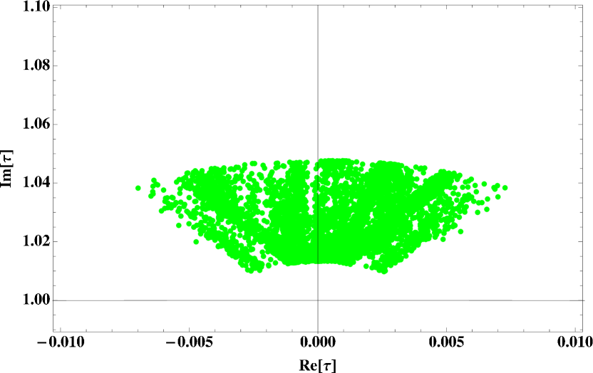
Figure 1: Allowed region on ${\rm Re}[\tau]$–${\rm Im}[\tau]$ plane consistent with three CKM mixing angles and $\delta_{CP}$. The black curve is the boundary of the fundamental region, $|\tau|=1$.

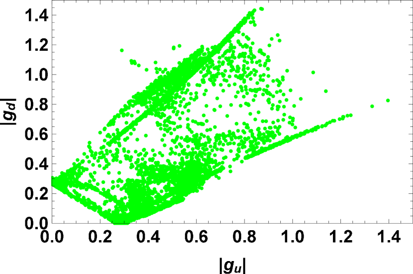
Figure 2: Allowed region on $|g_{u}|$–$|g_{d}|$ plane consistent with three CKM mixing angles and $\delta_{CP}$.

As seen in Table 2, the modulus $\tau$ is close to $i$. The deviation from $i$ is less than $5\%$. The modulus $\tau=i$ is a fixed point in the fundamental region of SL$(2,Z)$ under the transformation $S:\tau\rightarrow-1/\tau$. At $\tau=i$, CP is not violated as discussed in some works [41, 44, 86]. Indeed, we have succeeded to reproduce the observed CP violation at $\tau$ which is deviated a little bit from $\tau=i$.

In Fig. 1, we show the plot of ${\rm Re}[\tau]$ and ${\rm Im}[\tau]$, where output points are distributed overall in the $3\,\sigma$ range of the observed CKM elements, $|V_{us}|$, $|V_{cb}|$, $|V_{ub}|$ and $\delta_{CP}$ by choosing relevant $g_{u}$ and $g_{d}$. It is noticed that ${\rm Im}[\tau]=1-1.013$ is excluded while $|{\rm Re}[\tau]|$ is very small, less than $0.007$.

The fixed point $\tau=i$ is realized if there is a residual symmetry $\mathbb{Z}_{2}^{S}=\{I,S\}$, which is the subgroup of $A_{4}$. Then, the generator $S$ commutes with $M_{q}^{\dagger}M_{q}$ ,

$$\begin{aligned} \left[M_{q}^{\dagger}M_{q}\,,\,S\right]=0\,.\end{aligned}$$ (27)

Therefore, the mass matrix is expected to be diagonal in the diagonal base $\hat{S}$. However, the eigenvalue $-1$ of $S$ is degenerated, and so one pair off diagonal terms appear in $M_{q}^{\dagger}M_{q}$. We move to the diagonal base $\hat{S}$ by a unitary transformation as: $\hat{S}=USU^{\dagger}$, while the quark mass matrix $M_{q}$ is transformed as $M_{q}U^{\dagger}$. For the diagonal base $\hat{S}={\rm diag(-1,-1,1)}$, the unitary matrix is given as:

$$U=\begin{pmatrix}\frac{2}{\sqrt{6}}&-\frac{1}{\sqrt{6}}&-\frac{1}{\sqrt{6}}\\ 0&\frac{1}{\sqrt{2}}&\frac{1}{\sqrt{1}}\\ \frac{1}{\sqrt{3}}&\frac{1}{\sqrt{3}}&\frac{1}{\sqrt{3}}\end{pmatrix}.$$ (28)

Indeed, we have scanned model parameters around $\tau=i$ in the $\hat{S}$ base since it is easy to find hierarchical quark mass matrices consistent with the observed CKM matrix.

We also show the allowed region of absolute values, $|g_{u}|$ and $|g_{d}|$ in Fig.2. It is remarked that the non-vanishing $|g_{u}|$ or $|g_{d}|$ is required to reproduce the CKM elements, however, those are at most of order $1$. Indeed, the sum of $|g_{u}|$ and $|g_{d}|$ are larger than $0.25$, but smaller than $2.3$.

In Table 3, we show typical parameter sets and calculated CKM parameters. Ratios of $\alpha_{q}/\gamma_{q}$ and $\beta_{q}/\gamma_{q}$ $(q=u,d)$ correspond to the observed quark mass hierarchy.

	A sample set
$\tau$	$0.0007+1.041\,i$
$g_{u}$	$0.407-0.198\,i$
$g_{d}$	$0.745+0.176\,i$
$\alpha_{u}/\gamma_{u}$	$1.74\times 10^{2}$
$\beta_{u}/\gamma_{u}$	$1.11\times 10^{5}$
$\alpha_{d}/\gamma_{d}$	$1.88\times 10^{1}$
$\beta_{d}/\gamma_{d}$	$1.70\times 10^{-2}$
$|V_{us}|$	$0.226$
$|V_{cb}|$	$0.0487$
$|V_{ub}|$	$0.0027$
$\delta_{CP}$	$74.8^{\circ}$

Table 3: Numerical values of parameters and output of CKM parameters at a sample point.

We also present the mixing matrices of up-type quarks and down-type quarks for the sample in Table 3 in order to investigate the flavor structure of each quark mass matrix. After moving to the diagonal basis of $\hat{S}={\rm diag(-1,-1,1)}$ from the original one in Eq.(9), the mixing matrices of up- and down-quarks are given as:

$$\begin{aligned} V_{u}&\approx\begin{pmatrix}-0.529&0.848&-0.025\\ -0.820-0.200\,i&-0.514-0.125\,i&-0.091\\ -0.089-0.017\,i&-0.026-0.011\,i&0.995-0.016\,i\end{pmatrix}\ ,\\ V_{d}&\approx\begin{pmatrix}0.067&-0.645&-0.761\\ 0.067&-0.752+0.101\,i&0.643-0.086\,i\\ -0.995-0.016\,i&-0.094+0.005\,i&-0.008-0.006\,i\end{pmatrix}\ .\end{aligned}$$ (41)

The hierarchical flavor structure is partially seen as expected in the discussion of Eq.(28). After taking account of the degree of freedom of the permutation among $A_{4}$ triplet elements, ($q_{1},q_{2},q_{3}$), we can obtain the observed CKM matrix $V_{\rm CKM}=V_{u}^{\dagger}\,V_{d}$. Indeed, the permutation of $(d_{L},s_{L},b_{L})$ to $(s_{L},b_{L},d_{L})$, which corresponds the exchange of columns $(1,2,3)\to(2,3,1)$ in $V_{d}$, gives the observed CKM matrix with keeping $(u_{L},c_{L},t_{L})$.

In conclusion, our quark mass matrix with the $A_{4}$ modular symmetry can successfully reproduce the CKM mixing matrix completely. This successful result encourages us to investigate the lepton sector in the same framework. We discuss the lepton mass matrices with the $A_{4}$ modular symmetry in the next section.

5 Lepton mass matrix in the $A_{4}$ modular invariance

The modular $A_{4}$ invariance also gives the lepton mass matrix in terms of the modulus $\tau$ which is probably common both quarks and leptons if flavors of quarks and leptons are originated from a same two-dimensional compact space. The $A_{4}$ representations and weights are assigned for lepton fields relevantly as seen in Table 4, where the left-handed lepton doublets compose a $A_{4}$ triplet and the right-handed charged leptons are $A_{4}$ singlets. Weights of the left-handed leptons and the right-handed charged leptons are assigned like the quark ones in Table 4 (case I). In order to examine the quantitative dependence of our result on weights of the right-handed charged leptons, we also consider other choices of weights for the right-handed ones as cases II – V of Table 4.

	$L$	$(e^{c},\mu^{c},\tau^{c})$	$H_{u}$	$H_{d}$	$\bf Y_{3}^{(6)},Y_{3^{\prime}}^{(6)}$	$\bf Y_{3}^{(4)},Y_{1}^{(4)},Y_{1^{\prime}}^{(4)}$	$\bf Y_{3}^{(2)}$
$SU(2)$	$\bf 2$	$\bf 1$	$\bf 2$	$\bf 2$	$\bf 1$	$\bf 1$	$\bf 1$
$A_{4}$	$\bf 3$	(1, 1′′, 1′)	$\bf 1$	$\bf 1$	$\bf 3$	$\bf 3\,,\quad 1\,\quad 1^{\prime}$	$\bf 3$
$-k_{I}$	$-2$	I: $(-4,-2,0)$	0	0	$k=6$	$k=4$	$k=2$
		II: $(-4,\ \ 0,\,\ \ 0)$
		III: $(0,\ \ 0,\,\ \ 0)$
		IV: $(-2,\,\ 0,\,\ 0)$
		V: $(-2,\ -2,\,\ -2)$

Table 4: Assignments of representations and weights $-k_{I}$ for MSSM fields and modular forms.

Assign the left-handed charged leptons a $A_{4}$ triplet $L=(e_{L},\mu_{L},\tau_{L})$. Let us start with giving the charged lepton mass matrix $M_{E}$ in terms of modular forms of weight $2$, $4$ and $6$ in Eqs.(11), (LABEL:weight4) and (LABEL:weight6) as well as the quark sector. For the case I, it is presented as: where coefficients $\alpha_{e}$, $\beta_{e}$ and $\gamma_{e}$ are real parameters while $g_{e}$ is complex one. For the case II, it is given as On the other hand, a parameter $g_{e}$ of the mass matrix disappears for cases III, IV and V. They are respectively.

Suppose neutrinos to be Majorana particles. By using the Weinberg operator, the superpotential of the neutrino mass term, $w_{\nu}$ is given as:

$$w_{\nu} =-\frac{1}{\Lambda}(H_{u}H_{u}LL{\bf Y_{r}^{(k)}})_{\bf 1}~{},$$ (50)

where $\Lambda$ is a relevant cut off scale and the $A_{4}$ singlet component is extracted. Since the left-handed lepton doublet has weight $-2$, the superpotential is given in terms of modular forms of weight $4$, ${\bf Y_{3}^{(4)}}$, ${\bf Y_{1}^{(4)}}$ and ${\bf Y_{1^{\prime}}^{(4)}}$. By putting the vacuum expectation value of $H_{u}$ ($v_{u}$) and taking $L=(\nu_{e},\nu_{\mu},\nu_{\tau})$ for neutrinos, we have

$$w_{\nu} =\frac{v_{u}^{2}}{\Lambda}\left[\begin{pmatrix}2\nu_{e}\nu_{e}-\nu_{\mu}\nu_{\tau}-\nu_{\tau}\nu_{\mu}\\ 2\nu_{\tau}\nu_{\tau}-\nu_{e}\nu_{\mu}-\nu_{\mu}\nu_{\tau}\\ 2\nu_{\mu}\nu_{\mu}-\nu_{\tau}\nu_{e}-\nu_{e}\nu_{\tau}\end{pmatrix}\otimes{\bf Y_{3}^{(4)}}\right.$$

$$\left.+\ (\nu_{e}\nu_{e}+\nu_{\mu}\nu_{\tau}+\nu_{\tau}\nu_{\mu})\otimes g_{\nu 1}{\bf Y_{1}^{(4)}}+(\nu_{e}\nu_{\tau}+\nu_{\mu}\nu_{\mu}+\nu_{\tau}\nu_{e})\otimes g_{\nu 2}{\bf Y_{1^{\prime}}^{(4)}}\right]$$

$$= \frac{v_{u}^{2}}{\Lambda}\left[(2\nu_{e}\nu_{e}-\nu_{\mu}\nu_{\tau}-\nu_{\tau}\nu_{\mu})Y_{1}^{(4)}+(2\nu_{\tau}\nu_{\tau}-\nu_{e}\nu_{\mu}-\nu_{\mu}\nu_{e})Y_{3}^{(4)}+(2\nu_{\mu}\nu_{\mu}-\nu_{\tau}\nu_{e}-\nu_{e}\nu_{\tau})Y_{2}^{(4)}\right.$$

$$\left.+\ (\nu_{e}\nu_{e}+\nu_{\mu}\nu_{\tau}+\nu_{\tau}\nu_{\mu})g_{\nu 1}{\bf Y_{1}^{(4)}}+(\nu_{e}\nu_{\tau}+\nu_{\mu}\nu_{\mu}+\nu_{\tau}\nu_{e})g_{\nu 2}{\bf Y_{1^{\prime}}^{(4)}}\right]\ ,$$ (51)

where ${\bf Y_{3}^{(4)}}$, ${\bf Y_{1}^{(4)}}$ and ${\bf Y_{1^{\prime}}^{(4)}}$ are given in Eq. (LABEL:weight4), and $g_{\nu 1}$, $g_{\nu 2}$ are complex parameters. The neutrino mass matrix is written as follows:

$$M_{\nu}=\frac{v_{u}^{2}}{\Lambda}\left[\begin{pmatrix}2Y_{1}^{(4)}&-Y_{3}^{(4)}&-Y_{2}^{(4)}\\ -Y_{3}^{(4)}&2Y_{2}^{(4)}&-Y_{1}^{(4)}\\ -Y_{2}^{(4)}&-Y_{1}^{(4)}&2Y_{3}^{(4)}\end{pmatrix}+g_{\nu 1}{\bf Y_{1}^{(4)}}\begin{pmatrix}1&0&0\\ 0&0&1\\ 0&1&0\end{pmatrix}+g_{\nu 2}{\bf Y_{1^{\prime}}^{(4)}}\begin{pmatrix}0&0&1\\ 0&1&0\\ 1&0&0\end{pmatrix}\right]_{LL}\ .$$ (52)

Model parameters for cases I and II are $\alpha_{e}$, $\beta_{e}$, $\gamma_{e}$, $g_{e}$, $g_{\nu 1}$ and $g_{\nu 2}$ apart from the modulus $\tau$ while those of cases III, IV and V are $\alpha_{e}$, $\beta_{e}$, $\gamma_{e}$, $g_{\nu 1}$ and $g_{\nu 2}$. Parameters $\alpha_{e}$, $\beta_{e}$ and $\gamma_{e}$ are adjusted by the observed charged lepton masses. Therefore, the lepton mixing angles, the Dirac phase and Majorana phases are given by $g_{\nu 1}$, $g_{\nu 2}$ $(g_{e})$ in addition to the value of $\tau$. Since $\tau$ is scanned around $\tau=i$, where the quark CKM matrix is reproduced, we expect to get some predictions in the lepton sector. Practically, we scan $\tau$ in the regions of $|{\rm Re}[\tau]|\leq 0.1$ and ${\rm Im}[\tau]\leq 1.12$, which is close to the one of the quark sector . Indeed, our predictions are almost unchanged even if the scanned region of ${\rm Im}[\tau]$ is enlarged such as ${\rm Im}[\tau]\leq 1.13$.

observable	$3\,\sigma$ range for NH	$3\,\sigma$ range for IH
$\Delta m_{\rm atm}^{2}$	$(2.436$–$2.618)\times 10^{-3}\,{\rm eV}^{2}$	$-(2.419$–$2.601)\times 10^{-3}\,{\rm eV}^{2}$
$\Delta m_{\rm sol}^{2}$	$(6.79$–$8.01)\times 10^{-5}\,{\rm eV}^{2}$	$(6.79$–$8.01)\times 10^{-5}\,{\rm eV}^{2}$
$\sin^{2}\theta_{23}$	$0.433$–$0.609$	$0.436$–$0.610$
$\sin^{2}\theta_{12}$	$0.275$–$0.350$	$0.275$–$0.350$
$\sin^{2}\theta_{13}$	$0.02044$–$0.02435$	$0.02064$–$0.02457$

Table 5: The $3\,\sigma$ ranges of neutrino parameters from NuFIT 4.1 for NH and IH [87].

6 Modulus $\tau$ in the lepton mixing

We input charged lepton masses in order to constrain the model parameters. We take Yukawa couplings of charged leptons at the GUT scale $2\times 10^{16}$ GeV, where $\tan\beta=5$ is taken as well as quark Yukawa couplings [83, 84]:

$$y_{e}=(1.97\pm 0.024)\times 10^{-6},\quad y_{\mu}=(4.16\pm 0.050)\times 10^{-4},\quad y_{\tau}=(7.07\pm 0.073)\times 10^{-3},$$ (59)

where lepton masses are given by $m_{\ell}=y_{\ell}v_{H}$ with $v_{H}=174$ GeV. We also use the following lepton mixing angles and neutrino mass parameters, which are given by NuFit 4.1 in Table 5 [87]. Since there are two possible spectrum of neutrinos masses $m_{i}$, which are the normal hierarchy (NH), $m_{3}>m_{2}>m_{1}$, and the inverted hierarchy (IH), $m_{2}>m_{1}>m_{3}$, we investigate both cases.

Neutrino masses and the PMNS matrix $U_{\rm PMNS}$ [68, 69] are obtained by diagonalizing $M_{E}^{\dagger}M_{E}$ and $M_{\nu}^{*}M_{\nu}$. We also investigate the sum of three neutrino masses $\sum m_{i}$ in our model since it is constrained by the recent cosmological data, [85, 88, 89]. The effective mass for the $0\nu\beta\beta$ decay is given as follows:

$$\langle m_{ee}\rangle=\left|m_{1}c_{12}^{2}c_{13}^{2}+m_{2}s_{12}^{2}c_{13}^{2}e^{i\alpha_{21}}+m_{3}s_{13}^{2}e^{i(\alpha_{31}-2\delta^{\ell}_{CP})}\right|\ ,$$ (60)

where $\delta^{\ell}_{CP}$ is the Dirac phase of leptons, and $\alpha_{21}$, $\alpha_{31}$ are Majorana phases (see Appendix B).

Let us discuss numerical results for NH of neutrino masses in the case I of Eq.(LABEL:ME642) like the quark sector. After inputting charged lepton masses, parameters $\tau$, $g_{e}$, $g_{\nu 1}$ and $g_{\nu 2}$ are constrained by four observed quantities; three mixing angles of leptons and observed mass ratio $\Delta m_{\rm sol}^{2}/\Delta m_{\rm atm}^{2}$.

At first, we show the allowed region on the ${\rm Re}[\tau]$–${\rm Im}[\tau]$ plane in Fig. 3. Observed three mixing angles of leptons are reproduced at cyan, blue and red points. At cyan points, the sum of neutrino masses is consistent with the cosmological upper-bound $120$ meV. Red points denote common values of $\tau$ in both quarks and leptons. All allowed points are restricted in ${\rm Im}[\tau]\leq 1.08$ and $|{\rm Re}[\tau]|\leq 0.08$, that is around $\tau=i$. The red region does not satisfy $\sum m_{i}\leq 120$meV unless it expands to $|{\rm Re}[\tau]|\simeq 0.06$ or ${\rm Im}[\tau]\simeq 1.07$. In the region of $\tau$ in Fig. 1, we discuss the neutrino masses and the CP violating phase $\delta_{CP}^{\ell}$.

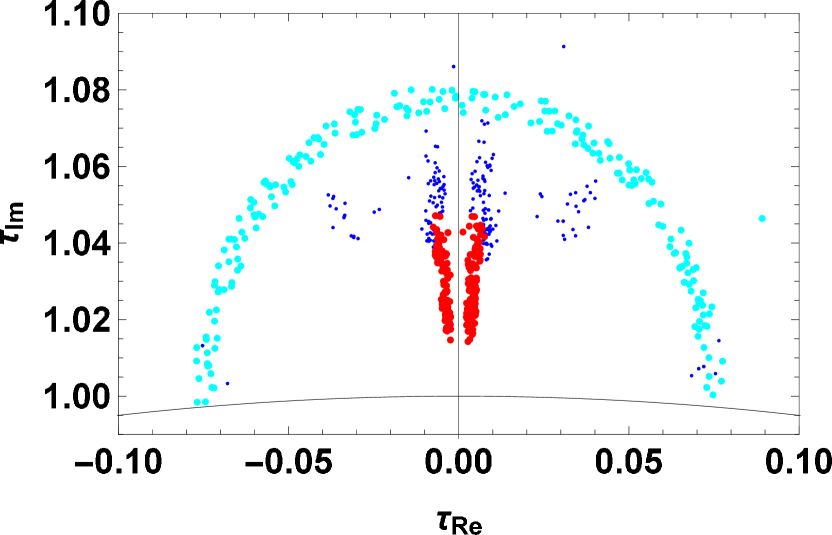
Figure 3: Allowed region on ${\rm Re}[\tau]$–${\rm Im}[\tau]$ plane for NH in the case I of $M_{E}$. Observed mixing angles are reproduced at cyan, blue and red points. At cyan points, the sum of neutrino masses is below $120$ meV. The solid curve is the boundary of the fundamental region, $|\tau|=1$.

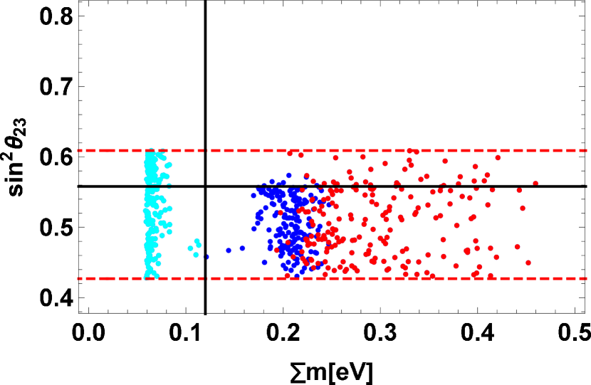
Figure 4: Allowed region on $\sum m_{i}$–$\sin^{2}\theta_{23}$ plane, where horizontal solid line denotes observed best-fit value, red dashed-lines denote the bound of $3\sigma$ interval, and vertical line is the cosmological bound, for NH in the case I of $M_{E}$. Color of points correspond to $\tau$ in Fig.3.

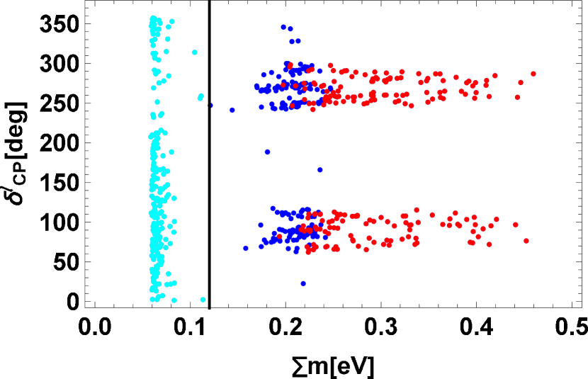
Figure 5: Allowed region on the $\sum m_{i}$–$\delta_{CP}^{\ell}$ plane, where the vertical line is the cosmological bound, for NH in the case I of $M_{E}$. Colors of points correspond to $\tau$ in Fig.3.

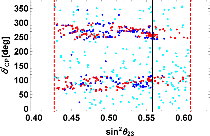
Figure 6: The correlation of $\sin^{2}\theta_{23}$ and $\delta_{CP}^{\ell}$, where the solid line denotes observed best-fit value and red dashed-lines denote the bound of $3\sigma$ interval, for NH in the case I of $M_{E}$.

We show the allowed region on the $\sum m_{i}$–$\sin^{2}\theta_{23}$ plane in Fig. 4, where colors (cyan, blue and red) of points correspond to points of $\tau$ in Fig. 3. The sum of neutrino masses is constrained by the cosmological upper-bound as seen in Fig. 4. The minimal cosmological model, ${\rm\Lambda CDM}+\sum m_{i}$, provides a tight bound for the sum of neutrino masses, $\sum m_{i}<120$ meV [88, 89] although it becomes weaker when the data are analysed in the context of extended cosmological models [85]. It is noticed that red points are in $\sum m_{i}\geq 190$meV in Fig. 4. If these points will be completely exculded by the robust cosmological upper-bound of the sum of neutrino masses in the near future, the common region of $\tau$ between quarks and leptons vanishes. The calculated $\sin^{2}\theta_{23}$ is distributed overall in the $3\,\sigma$ range of NuFIT 4.1 [87] below $\sum m_{i}=120$ meV.

We show the allowed region on the $\sum m_{i}$–$\delta_{CP}^{\ell}$ plane in Fig. 5. In the region of red points, $\delta_{CP}^{\ell}$ is predicted to be in the restricted ranges, $60^{\circ}$–$120^{\circ}$ and $240^{\circ}$–$300^{\circ}$. Below $\sum m_{i}=120$ meV (cyan points), $\delta_{CP}^{\ell}$ is allowed in $[0,\,2\pi]$. In Fig. 6, we plot $\delta_{CP}^{\ell}$ versus $\sin^{2}\theta_{23}$ in order to see their correlation. It is found that there is no distinct correlation between them. Around the best fit point of $\sin^{2}\theta_{23}$, the predicted $\delta_{CP}^{\ell}$ is also in $[0,\,2\pi]$ below $\sum m_{i}=120$ meV (cyan points).

It is also noted that the effective mass of the $0\nu\beta\beta$ decay $\langle m_{ee}\rangle$ is predicted in $1.5$–$28$ meV below $\sum m_{i}=120$ meV.

	A sample set
$\tau$	$0.028+1.075\,i$
$g_{\nu 1}$	$-1.156-0.373\,i$
$g_{\nu 2}$	$-0.617-0.441\,i$
$g_{e}$	$-0.736-0.430\,i$
$\alpha_{e}/\gamma_{e}$	$11.6$
$\beta_{e}/\gamma_{e}$	$3.92\times 10^{-3}$
$\sin^{2}\theta_{12}$	$0.314$
$\sin^{2}\theta_{23}$	$0.563$
$\sin^{2}\theta_{13}$	$0.0233$
$\delta_{CP}^{\ell}$	$278^{\circ}$
$\sum m_{i}$	$72.2$ meV
$\langle m_{ee}\rangle$	$8.0$ meV

Table 6: Numerical values of parameters and output of PMNS parameters at a sample point.

In Table 6, we show a typical parameter set and the output of observables, which is chosen among cyan points (below $\sum m_{i}=120$ meV). Ratios of $\alpha_{e}/\gamma_{e}$ and $\beta_{e}/\gamma_{e}$ correspond to the observed charged lepton mass hierarchy.

As discussed in the quark sector, Eqs. (27) and (28), we have scanned model parameters around $\tau=i$ in the diagonal base of the generator $S$, where eigenvalues are ${\rm diag(1,-1,-1)}$ in this case. The unitary matrix corresponding to Eq.(28) is obtained by its permutation of rows $1\to 3\to 2\to 1$. Thanks to this base, it is easy to find hierarchical mixing matrices of the charged lepton. In this base, we present the mixing matrices of charged leptons and neutrinos for a sample of Table 6 as:

$$\begin{aligned} U_{\ell}&\approx\begin{pmatrix}0.627+0.759\,i&-0.017-0.077\,i&-0.159-0.005\,i\\ -0.107-0.064\,i&-0.560+0.237\,i&-0.782-0.063\,i\\ -0.108-0.064\,i&0.221-0.759\,i&-0.404+0.444\,i\\ \end{pmatrix}\ ,\\ U_{\nu}&\approx\begin{pmatrix}-0.101-0.856\,i&-0.190+0.470\,i&0.008-0.001\,i\\ -0.488-0.107\,i&-0.640-0.557\,i&-0.162+0.068\,i\\ 0.078+0.035\,i&0.081+0.131\,i&-0.978+0.116\,i\end{pmatrix}\ .\end{aligned}$$ (74)

The PMNS matrix is given by $U_{\rm PMNS}=U_{\ell}^{\dagger}\,U_{\nu}$. It is noticed that the large $\theta_{23}$ comes from the charged lepton mass matrix while the large $\theta_{12}$ comes from the neutrino one.

In order to study the quantitative dependence of our result on weights of the right-handed charged leptons, we discuss other cases of those weights in Table 4, in which the mass matrix of the charged lepton is different from the quark one. Let us begin to examine the case II of Table 4, which presents the charged lepton mass matrix in Eq.(LABEL:ME622). Indeed, we obtain the common region of $\tau$ for quarks and leptons in this case. Let us show the allowed region ${\rm Re}[\tau]$–${\rm Im}[\tau]$ plane in Fig. 7. Observed three mixing angles of leptons are reproduced at cyan, blue and red points. At cyan points, the sum of neutrino masses is below the cosmological upper-bound $120$ meV. Red points denote common values of $\tau$ in both quarks and leptons. The red region does not satisfy $\sum m_{i}\leq 120$meV unless it expands to $|{\rm Re}[\tau]|\simeq 0.03$ and ${\rm Im}[\tau]\simeq 1.06$.

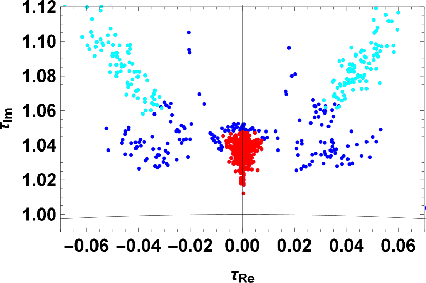
Figure 7: Allowed region on ${\rm Re}[\tau]$–${\rm Im}[\tau]$ plane for NH in the case II of $M_{E}$. Observed mixing angles are reproduced at cyan, blue and red points. At cyan points, the sum of neutrino masses is below $120$ meV. The solid curve is the boundary of the fundamental region, $|\tau|=1$.

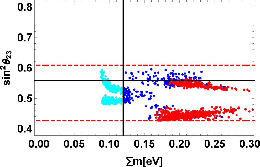
Figure 8: Allowed region on $\sum m_{i}$–$\sin^{2}\theta_{23}$ plane, where horizontal solid line denotes observed best-fit one, red dashed-lines denote the bound of $3\sigma$ interval, and vertical line is the cosmological bound, for NH in the case II of $M_{E}$. Colors of points correspond to $\tau$ in Fig.7.

We show the allowed region on the $\sum m_{i}$–$\sin^{2}\theta_{23}$ plane in Fig. 8, where colors (cyan, blue and red) of points correspond to points of $\tau$ in Fig.8. The sum of neutrino masses is constrained by the cosmological upper-bound as seen in Fig. 7. It is noticed that red points are in $\sum m_{i}\geq 165$meV. If these points will be completely excluded by the robust cosmological upper-bound of the sum of neutrino masses in the near future, the common region of $\tau$ between quarks and leptons vanishes. Below $\sum m_{i}=120$meV, $\sin^{2}\theta_{23}$ is predicted in the range of $0.48$–$0.60$.

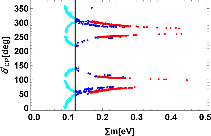
Figure 9: Allowed region on $\sum m_{i}$–$\delta_{CP}^{\ell}$ plane, where the vertical line is the cosmological bound, for NH in the case II of $M_{E}$. Colors of points correspond to $\tau$ in Fig.7.

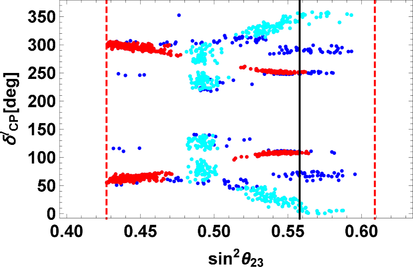
Figure 10: The correlation of $\sin^{2}\theta_{23}$ and $\delta_{CP}^{\ell}$, where the solid line denotes observed best-fit value and red dashed-lines denote the bound of $3\sigma$ interval, for NH in the case II of $M_{E}$.

We show the allowed region on the $\sum m_{i}$–$\delta_{CP}^{\ell}$ plane in Fig. 9. In the region of red points, $\delta_{CP}^{\ell}$ is predicted to be in the restricted ranges, $55^{\circ}$–$75^{\circ}$, $100^{\circ}$–$110^{\circ}$, $250^{\circ}$–$260^{\circ}$ and $285^{\circ}$–$305^{\circ}$. Below $\sum m_{i}=120$ meV, $\delta_{CP}^{\ell}$ is rather wide ranges in $0^{\circ}$–$100^{\circ}$, $110^{\circ}$–$135^{\circ}$, $225^{\circ}$–$250^{\circ}$ and $260^{\circ}$–$360^{\circ}$. We plot $\delta_{CP}^{\ell}$ versus $\sin^{2}\theta_{23}$ in Fig. 10. It is found a clear correlation between them in contrast with the case I. At the best fit point of $\sin^{2}\theta_{23}$, $\delta_{CP}^{\ell}$ is predicted to be $0^{\circ}$–$20^{\circ}$ and $340^{\circ}$–$360^{\circ}$ below $\sum m_{i}=120$ meV (cyan points).

We can also predict the effective mass of the $0\nu\beta\beta$ decay $\langle m_{ee}\rangle$. It is in $16$–$31$ meV below $\sum m_{i}=120$ meV.

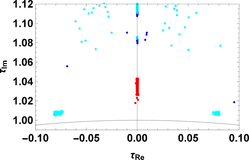
Figure 11: Allowed region on ${\rm Re}[\tau]$–${\rm Im}[\tau]$ plane for NH in the case III of $M_{E}$. Observed mixing angles are reproduced at cyan, blue and red points. At cyan points, the sum of neutrino masses is below $120$ meV. The solid curve is the boundary of the fundamental region, $|\tau|=1$.

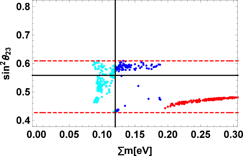
Figure 12: Allowed region on $\sum m_{i}$–$\sin^{2}\theta_{23}$ plane, where horizontal solid line denotes observed best-fit one, red dashed-lines denote the bound of $3\sigma$ interval, and vertical line is the cosmological bound, for NH in the case III of $M_{E}$. Colors of points correspond to $\tau$ in Fig.11.

As seen in the charged lepton mass matrix of Eqs. (LABEL:ME642) and (LABEL:ME622), there is a complex parameter $g_{e}$ in addition to $g_{\nu 1}$ and $g_{\nu 2}$ of the neutrino sector for cases I and II. This additional parameter $g_{e}$ gives the disadvantage to predict the CP violating phase. Indeed, $\delta_{CP}^{\ell}$ is predicted in the wide range for cases I and II as seen in Figs. 5 and 9. In order to improve the predictability of the model, cases III, IV and V provide attractive mass matrices .

The mass matrix of Eq. (LABEL:ME222) (case III) is the simplest one although this texture is excluded in the quark sector as discussed in Eq. (15). Remarkably, there exists a common region of $\tau$ for quarks and leptons in this case. Let us show the allowed region on the ${\rm Re}[\tau]$–${\rm Im}[\tau]$ plane in Fig. 11. Observed three mixing angles of leptons are reproduced at cyan, blue and red points. The common region of $\tau$ in both quarks and leptons are presented by red points. At cyan points, the sum of neutrino masses is below the cosmological upper-bound $120$ meV.

We show the allowed region on the $\sum m_{i}$–$\sin^{2}\theta_{23}$ plane in Fig. 12, where colors (cyan, blue and red) of points correspond to points of $\tau$ in Fig. 11. It is found red points to be larger than $\sum m_{i}=195$meV. The common region of $\tau$ in quarks and leptons vanishes if the cosmological upper-bound of the sum of neutrino masses is the robust one. Below $\sum m_{i}=120$meV (cyan points), $\sin^{2}\theta_{23}$ is predicted in the range of $0.46$–$0.60$.

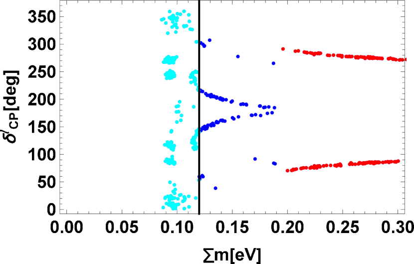
Figure 13: Allowed region on the $\sum m_{i}$–$\delta_{CP}^{\ell}$ plane, where the vertical line is the cosmological bound, for NH in the case III of $M_{E}$. Colors of points correspond to points of $\tau$ in Fig.11.

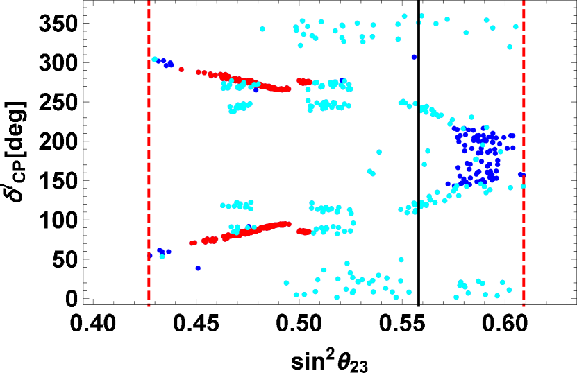
Figure 14: The correlation of $\sin^{2}\theta_{23}$ and $\delta_{CP}^{\ell}$, where the black line denotes observed best-fit value and red dashed-lines denote the bound of $3\sigma$ interval, for NH in the case III of $M_{E}$.

We show the allowed region on the $\sum m_{i}$–$\delta_{CP}^{\ell}$ plane in Fig. 13. In the region of red points, $\delta_{CP}^{\ell}$ is predicted to be in the restricted ranges, $70^{\circ}$–$90^{\circ}$ and $270^{\circ}$–$290^{\circ}$. However, below $\sum m_{i}=120$ meV, the predicted region of $\delta_{CP}^{\ell}$ is expanded.

We plot $\delta_{CP}^{\ell}$ versus $\sin^{2}\theta_{23}$ in Fig. 14. It is found a clear correlation between them as well as the case II. At the best fit point of $\sin^{2}\theta_{23}$, $\delta_{CP}^{\ell}$ is predicted to be $110^{\circ}$–$125^{\circ}$ and $235^{\circ}$–$250^{\circ}$ below $\sum m_{i}=120$ meV (cyan points), which is remarkably different from the ones in cases I and II. We can also predict the effective mass of the $0\nu\beta\beta$ decay $\langle m_{ee}\rangle$. It is in $15$–$30$ meV below $\sum m_{i}=120$ meV.

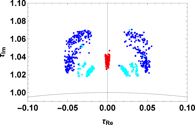
Figure 15: Allowed region on ${\rm Re}[\tau]$–${\rm Im}[\tau]$ plane for NH in the case IV of $M_{E}$. Observed mixing angles are reproduced at cyan, blue and red points. At cyan points, the sum of neutrino masses is below $120$ meV. The solid curve is the boundary of the fundamental region, $|\tau|=1$.

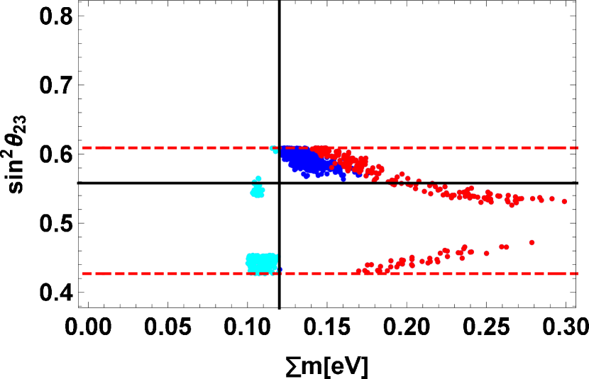
Figure 16: Allowed region on $\sum m_{i}$–$\sin^{2}\theta_{23}$ plane, where horizontal solid line denotes observed best-fit value, dashed-lines denote the bound of $3\sigma$ interval, and vertical line is the cosmological bound, for NH in the case IV of $M_{E}$. Colors of points correspond to $\tau$ in Fig.15.

For the case IV in Eq. (LABEL:ME422), where the charged lepton mass matrix is composed of both weight 2 and 4 modular forms contrast to the case III, we obtain the common region of $\tau$ in quarks and leptons. Let us show the allowed region ${\rm Re}[\tau]$–${\rm Im}[\tau]$ plane in Fig. 15. Observed three mixing angles of leptons are reproduced at cyan, blue and red points. At cyan points, the sum of neutrino masses is below the cosmological upper-bound $120$ meV. Red points denote common values of $\tau$ in both quarks and leptons. As seen in Fig. 15, cyan points are not so far away from the red region.

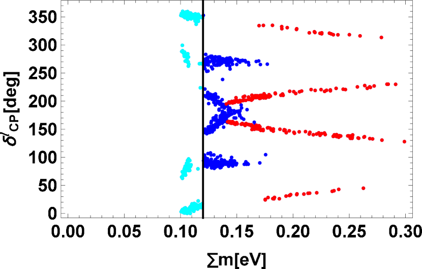
Figure 17: Allowed region on the $\sum m_{i}$–$\delta_{CP}^{\ell}$ plane, where the vertical line is the cosmological bound, for NH in the case IV of $M_{E}$. Colors of points correspond to $\tau$ in Fig.15.

Figure 18: The correlation of $\sin^{2}\theta_{23}$ and $\delta_{CP}^{\ell}$, where the solid line denotes observed best-fit value and red dashed-lines denote the bound of $3\sigma$ interval, for NH in the case IV of $M_{E}$.

We show the allowed region on the $\sum m_{i}$–$\sin^{2}\theta_{23}$ plane in Fig. 16, where colors (cyan, blue and red) of points correspond to points of $\tau$ in Fig.15. It is found red points to be larger than $\sum m_{i}=140$meV. The common region of $\tau$ in quarks and leptons vanishes under $\sum m_{i}=120$meV. If the cosmological upper-bound of the sum of neutrino masses is allowed up to $\sum m_{i}=160$meV [85], $\sin^{2}\theta_{23}$ is predicted to be $0.58$–$0.61$ at the common $\tau$ of quarks and leptons.

We show the allowed region on the $\sum m_{i}$–$\delta_{CP}^{\ell}$ plane in Fig. 17. The predicted $\delta_{CP}^{\ell}$ is in $150^{\circ}$–$160^{\circ}$ and $200^{\circ}$–$210^{\circ}$ at the common $\tau$ of quarks and leptons. However, below $\sum m_{i}=120$ meV, the predicted $\delta_{CP}^{\ell}$ (cyan points) is $0^{\circ}$–$20^{\circ}$, $60^{\circ}$–$100^{\circ}$, $260^{\circ}$–$300^{\circ}$ and $340^{\circ}$–$360^{\circ}$.

We plot $\delta_{CP}^{\ell}$ versus $\sin^{2}\theta_{23}$ in Fig. 18. It is found a clear correlation between them as well as cases II and III. At the best fit point of $\sin^{2}\theta_{23}$, $\delta_{CP}^{\ell}$ is predicted to be $90^{\circ}$ and $270^{\circ}$ below $\sum m_{i}=120$ meV (cyan points).

Finally, the effective mass of the $0\nu\beta\beta$ decay $\langle m_{ee}\rangle$ is in $22$–$30$ meV below $\sum m_{i}=120$ meV.

For the case V in Eq.(LABEL:ME444), where the charged lepton mass matrix is composed of only weight 4 modular forms, there is no common region of $\tau$ for quarks and leptons. Observed three mixing angles of leptons are not reproduced unless the sum of neutrino masses is larger than $450$ meV, which is far away from the cosmological upper-bound $120$ meV. Therefore, we omit to show numerical results for this case.

In Table 7, we summarize characteristic results of cases I–V including ones of IH. In our numerical calculations, we have not included the RGE effects in the lepton mixing angles and neutrino mass ratio $\Delta m_{\rm sol}^{2}/\Delta m_{\rm atm}^{2}$. We suppose that those corrections are very small between the electroweak and GUT scales for NH of neutrino masses. This assumption is justified very well in the case of $\tan\beta\leq 5$ as far as the sum of neutrino masses is less than a few hundred meV [27, 90].

Cases		I	II	III	I V	V
common $\tau$	NH	$\bigcirc$	$\bigcirc$	$\bigcirc$	$\bigcirc$	$\times$
of quarks/leptons	IH	$\bigcirc$	$\times$	$\bigcirc$	$\times$	$\times$
$\sum m_{i}$	NH	$\geq 190$ meV	$\geq 165$ meV	$\geq 195$ meV	$\geq 140$ meV	—
at common $\tau$	IH	$\geq 680$ meV	—	$\geq 420$ meV	—	—
$\delta_{CP}^{\ell}$	NH	$0$–$360^{\circ}$	$0$–$20^{\circ}$,	$110^{\circ}$–$125^{\circ}$,	$0$–$20^{\circ}$, $340^{\circ}$–$360^{\circ}$,	—
at best fit of $\sin^{2}\theta_{23}$			$340^{\circ}$-$360^{\circ}$	$235^{\circ}$–$250^{\circ}$	$60^{\circ}$-$100^{\circ}$, $260$–$300^{\circ}$
in $\sum m_{i}\leq 120$ meV	IH	—	—	—	—	—
$\langle m_{ee}\rangle$	NH	$1.5$–$28$ meV	$16$–$31$ meV	$15$–$30$ meV	$22$–$30$ meV	—
in $\sum m_{i}\leq 120$ meV	IH	—	—	$22$–$24$ meV	—	—

Table 7: Summary of characteristic predictions for NH and IH of cases I – V.

Finally, we discuss briefly the case of IH of neutrino masses. Indeed, there is the common region of $\tau$ in quarks and leptons for the case I of Eq.(LABEL:ME642), where the predicted $\sin^{2}\theta_{23}$ is larger than $0.6$, and $\delta_{CP}^{\ell}$ is around $70^{\circ}$ and $290^{\circ}$. However, this case is completely excluded because the sum of neutrino masses is larger than $680$ meV. Observed three mixing angles of leptons are not reproduced below $\sum m_{i}\leq 600$ meV. In the case II of Eq.(LABEL:ME622), there is no common region of $\tau$ in quarks and leptons. Observed three mixing angles of leptons are not reproduced unless the sum of neutrino masses is larger than $200$ meV. In the case III, it is found the common region of $\tau$ in quarks and leptons, but the sum of neutrino masses is larger than $420$ meV. Observed three mixing angles of leptons are reproduced below $\sum m_{i}\leq 120$ meV, where $\sin^{2}\theta_{23}\simeq 0.49$–$0.52$, $\delta_{CP}^{\ell}=50^{\circ}$–$60^{\circ}$, $160^{\circ}$–$170^{\circ}$, $190^{\circ}$–$200^{\circ}$, $300^{\circ}$–$310^{\circ}$, and $\langle m_{ee}\rangle=22$-$24$ meV. For cases IV and V, there are no common regions of $\tau$ in quarks and leptons. Below $\sum m_{i}\leq 120$ meV, observed three mixing angles of leptons are not reproduced in our scan regions of $|{\rm Re}[\tau]|\leq 0.1$ and ${\rm Im}[\tau]\leq 1.12$. In conclusion, IH of neutrino masses is unfavorable in our model. We summarize the results of IH in Table 7.

7 Summary and discussions

In this work, we have studied both quark and lepton mass matrices in the $A_{4}$ modular symmetry towards the unification of quark and lepton flavors. If flavors of quarks and leptons are originated from a same two-dimensional compact space, the quarks and leptons have same flavor symmetry and the common modulus $\tau$.

The viable quark mass matrices are composed of modular forms of weights $2$, $4$ and $6$. It is remarked that $\tau$ is close to $i$, which is a fixed point in the fundamental region of SL$(2,Z)$, and the CP symmetry is not violated. Indeed, we reproduce the observed CP violation of the quark sector at $\tau$ which is deviated a little bit from $\tau=i$.

The charged lepton mass matrix is also given by using modular forms of weights $2$, $4$ and $6$. In order to study the quantitative dependence of our result on weights of the right-handed charged leptons, we have examined five cases I–V of them. The neutrino mass matrix is generated in terms of the modular forms of weight $4$ through the Weinberg operator.

Our lepton mass matrices are also consistent with the observed mixing angles at $\tau$ close to $i$ for NH of neutrino masses. It is found that allowed regions of $\tau$ of quarks and leptons overlap each other for all cases of the charged lepton mass matrix. The sum of neutrino masses is crucial to test the common $\tau$ for quarks and leptons. The predicted minimal sum of neutrino masses $\sum m_{i}$ is $140$ meV at the common $\tau$ in the case IV. If the cosmological upper-bound of the sum of neutrino masses, $120$ meV will be confirmed, the common region of $\tau$ of quarks and leptons vanishes. However, the allowed region of $\tau$ in both quark and lepton sectors could be shifted to a certain extent by some corrections such as the SUSY breaking effect through threshold corrections to masses and mixing angles. The appreciable shift of $\tau$ could be also occurred by the modification of the quark and lepton mass matrices. We need further investigation of the mass matrices to reproduce the observed CKM and PMNS on the common $\tau$.

As well known, the modulus $\tau=i$ is a fixed point, which is invariant in the $\mathbb{Z}_{2}^{S}=\{I,S\}$ group. In our numerical results, the modulus $\tau$ is fixed close to $\tau=i$, which suggests the approximate residual symmetry in the quark and lepton mass matrices. Some corrections could violate the exact symmetry. The group theoretical investigation will be presented in the near future. It is also emphasized that the spontaneous CP violation in Type IIB string theory is possibly realized nearby $\tau=i$, where the moduli stabilization as well as the calculation of Yukawa couplings is performed in a controlled way [91]. Thus, our phenomenological result of $\tau$ may be favored in the theoretical investigation.

It may be useful to note that IH of neutrino masses is unfavorable in our framework. Our study provides a phenomenological new aspect towards the unification of the quark and lepton flavors in terms of the modulus $\tau$.

Appendix

Appendix A Tensor product of $A_{4}$ group

We take the generators of $A_{4}$ group as follows:

$$\begin{aligned} S=\frac{1}{3}\begin{pmatrix}-1&2&2\\ 2&-1&2\\ 2&2&-1\end{pmatrix},\end{aligned}\qquad\begin{aligned} T=\begin{pmatrix}1&0&0\\ 0&\omega&0\\ 0&0&\omega^{2}\end{pmatrix},\end{aligned}$$ (85)

where $\omega=e^{i\frac{2}{3}\pi}$ for a triplet. In this base, the multiplication rule of the $A_{4}$ triplet is

$$\begin{pmatrix}a_{1}\\ a_{2}\\ a_{3}\end{pmatrix}_{\bf 3}\otimes\begin{pmatrix}b_{1}\\ b_{2}\\ b_{3}\end{pmatrix}_{\bf 3} =\left(a_{1}b_{1}+a_{2}b_{3}+a_{3}b_{2}\right)_{\bf 1}\oplus\left(a_{3}b_{3}+a_{1}b_{2}+a_{2}b_{1}\right)_{{\bf 1}^{\prime}}$$

$$\oplus\left(a_{2}b_{2}+a_{1}b_{3}+a_{3}b_{1}\right)_{{\bf 1}^{\prime\prime}}$$

$$\oplus\frac{1}{3}\begin{pmatrix}2a_{1}b_{1}-a_{2}b_{3}-a_{3}b_{2}\\ 2a_{3}b_{3}-a_{1}b_{2}-a_{2}b_{1}\\ 2a_{2}b_{2}-a_{1}b_{3}-a_{3}b_{1}\end{pmatrix}_{{\bf 3}}\oplus\frac{1}{2}\begin{pmatrix}a_{2}b_{3}-a_{3}b_{2}\\ a_{1}b_{2}-a_{2}b_{1}\\ a_{3}b_{1}-a_{1}b_{3}\end{pmatrix}_{{\bf 3}\ }\ ,$$

$${\bf 1}\otimes{\bf 1}={\bf 1}\ ,\qquad {\bf 1^{\prime}}\otimes{\bf 1^{\prime}}={\bf 1^{\prime\prime}}\ ,\qquad{\bf 1^{\prime\prime}}\otimes{\bf 1^{\prime\prime}}={\bf 1^{\prime}}\ ,\qquad{\bf 1^{\prime}}\otimes{\bf 1^{\prime\prime}}={\bf 1}\ .$$ (86)

More details are shown in the review [6, 7].

Appendix B Majorana and Dirac phases and $\langle m_{ee}\rangle$ in $0\nu\beta\beta$ decay

Supposing neutrinos to be Majorana particles, the PMNS matrix $U_{\text{PMNS}}$ [68, 69] is parametrized in terms of the three mixing angles $\theta_{ij}$ $(i,j=1,2,3;~{}i<j)$, one CP violating Dirac phase $\delta_{\text{CP}}$ and two Majorana phases $\alpha_{21}$, $\alpha_{31}$ as follows:

$$U_{\text{PMNS}}=\begin{pmatrix}c_{12}c_{13}&s_{12}c_{13}&s_{13}e^{-i\delta^{\ell}_{\text{CP}}}\\ -s_{12}c_{23}-c_{12}s_{23}s_{13}e^{i\delta^{\ell}_{\text{CP}}}&c_{12}c_{23}-s_{12}s_{23}s_{13}e^{i\delta^{\ell}_{\text{CP}}}&s_{23}c_{13}\\ s_{12}s_{23}-c_{12}c_{23}s_{13}e^{i\delta^{\ell}_{\text{CP}}}&-c_{12}s_{23}-s_{12}c_{23}s_{13}e^{i\delta^{\ell}_{\text{CP}}}&c_{23}c_{13}\end{pmatrix}\begin{pmatrix}1&0&0\\ 0&e^{i\frac{\alpha_{21}}{2}}&0\\ 0&0&e^{i\frac{\alpha_{31}}{2}}\end{pmatrix},$$ (87)

where $c_{ij}$ and $s_{ij}$ denote $\cos\theta_{ij}$ and $\sin\theta_{ij}$, respectively.

The rephasing invariant CP violating measure of leptons [92, 93] is defined by the PMNS matrix elements $U_{\alpha i}$. It is written in terms of the mixing angles and the CP violating phase as:

$$J_{CP}=\text{Im}\left[U_{e1}U_{\mu 2}U_{e2}^{\ast}U_{\mu 1}^{\ast}\right]=s_{23}c_{23}s_{12}c_{12}s_{13}c_{13}^{2}\sin\delta^{\ell}_{\text{CP}}~{},$$ (88)

where $U_{\alpha i}$ denotes the each component of the PMNS matrix.

There are also other invariants $I_{1}$ and $I_{2}$ associated with Majorana phases

$$I_{1}=\text{Im}\left[U_{e1}^{\ast}U_{e2}\right]=c_{12}s_{12}c_{13}^{2}\sin\left(\frac{\alpha_{21}}{2}\right)~{},\quad I_{2}=\text{Im}\left[U_{e1}^{\ast}U_{e3}\right]=c_{12}s_{13}c_{13}\sin\left(\frac{\alpha_{31}}{2}-\delta^{\ell}_{\text{CP}}\right)~{}.$$ (89)

We can calculate $\delta^{\ell}_{\text{CP}}$, $\alpha_{21}$ and $\alpha_{31}$ with these relations by taking account of

$$\cos\delta^{\ell}_{CP}=\frac{|U_{\tau 1}|^{2}-s_{12}^{2}s_{23}^{2}-c_{12}^{2}c_{23}^{2}s_{13}^{2}}{2c_{12}s_{12}c_{23}s_{23}s_{13}}~{},$$

$$\text{Re}\left[U_{e1}^{\ast}U_{e2}\right]=c_{12}s_{12}c_{13}^{2}\cos\left(\frac{\alpha_{21}}{2}\right)~{},\qquad\text{Re}\left[U_{e1}^{\ast}U_{e3}\right]=c_{12}s_{13}c_{13}\cos\left(\frac{\alpha_{31}}{2}-\delta^{\ell}_{\text{CP}}\right)~{}.$$ (90)

In terms of these parametrization, the effective mass for the $0\nu\beta\beta$ decay is given as follows:

$$\langle m_{ee}\rangle=\left|m_{1}c_{12}^{2}c_{13}^{2}+m_{2}s_{12}^{2}c_{13}^{2}e^{i\alpha_{21}}+m_{3}s_{13}^{2}e^{i(\alpha_{31}-2\delta^{\ell}_{CP})}\right|\ .$$ (91)

References

- [1] S. Pakvasa and H. Sugawara, Phys. Lett. 73B (1978) 61.
- [2] F. Wilczek and A. Zee, Phys. Lett. 70B (1977) 418 Erratum: [Phys. Lett. 72B (1978) 504].
- [3] M. Fukugita, M. Tanimoto and T. Yanagida, Phys. Rev. D 57 (1998) 4429 [hep-ph/9709388].
- [4] Y. Fukuda et al. [Super-Kamiokande Collaboration], Phys. Rev. Lett. 81 (1998) 1562 [hep-ex/9807003].
- [5] G. Altarelli and F. Feruglio, Rev. Mod. Phys. 82 (2010) 2701 [arXiv:1002.0211 [hep-ph]].
- [6] H. Ishimori, T. Kobayashi, H. Ohki, Y. Shimizu, H. Okada and M. Tanimoto, Prog. Theor. Phys. Suppl. 183 (2010) 1 [arXiv:1003.3552 [hep-th]].
- [7] H. Ishimori, T. Kobayashi, H. Ohki, H. Okada, Y. Shimizu and M. Tanimoto, Lect. Notes Phys. 858 (2012) 1, Springer.
- [8] D. Hernandez and A. Y. Smirnov, Phys. Rev. D 86 (2012) 053014 [arXiv:1204.0445 [hep-ph]].
- [9] S. F. King and C. Luhn, Rept. Prog. Phys. 76 (2013) 056201 [arXiv:1301.1340 [hep-ph]].
- [10] S. F. King, A. Merle, S. Morisi, Y. Shimizu and M. Tanimoto, New J. Phys. 16, 045018 (2014) [arXiv:1402.4271 [hep-ph]].
- [11] M. Tanimoto, AIP Conf. Proc. 1666 (2015) 120002.
- [12] S. F. King, Prog. Part. Nucl. Phys. 94 (2017) 217 [arXiv:1701.04413 [hep-ph]].
- [13] S. T. Petcov, Eur. Phys. J. C 78 (2018) no.9, 709 [arXiv:1711.10806 [hep-ph]].
- [14] F. Feruglio and A. Romanino, arXiv:1912.06028 [hep-ph].
- [15] E. Ma and G. Rajasekaran, Phys. Rev. D 64, 113012 (2001) [arXiv:hep-ph/0106291].
- [16] K. S. Babu, E. Ma and J. W. F. Valle, Phys. Lett. B 552, 207 (2003) [arXiv:hep-ph/0206292].
- [17] G. Altarelli and F. Feruglio, Nucl. Phys. B 720 (2005) 64 [hep-ph/0504165].
- [18] G. Altarelli and F. Feruglio, Nucl. Phys. B 741 (2006) 215 [hep-ph/0512103].
- [19] Y. Shimizu, M. Tanimoto and A. Watanabe, Prog. Theor. Phys. 126 (2011) 81 [arXiv:1105.2929 [hep-ph]].
- [20] S. T. Petcov and A. V. Titov, Phys. Rev. D 97 (2018) no.11, 115045 [arXiv:1804.00182 [hep-ph]].
- [21] S. K. Kang, Y. Shimizu, K. Takagi, S. Takahashi and M. Tanimoto, PTEP 2018, no. 8, 083B01 (2018) [arXiv:1804.10468 [hep-ph]].
- [22] F. Feruglio, doi:10.1142/9789813238053-0012 arXiv:1706.08749 [hep-ph].
- [23] R. de Adelhart Toorop, F. Feruglio and C. Hagedorn, Nucl. Phys. B 858, 437 (2012) [arXiv:1112.1340 [hep-ph]].
- [24] T. Kobayashi, K. Tanaka and T. H. Tatsuishi, Phys. Rev. D 98 (2018) no.1, 016004 [arXiv:1803.10391 [hep-ph]].
- [25] J. T. Penedo and S. T. Petcov, Nucl. Phys. B 939 (2019) 292 [arXiv:1806.11040 [hep-ph]].
- [26] P. P. Novichkov, J. T. Penedo, S. T. Petcov and A. V. Titov, JHEP 1904 (2019) 174 [arXiv:1812.02158 [hep-ph]].
- [27] J. C. Criado and F. Feruglio, SciPost Phys. 5 (2018) no.5, 042 [arXiv:1807.01125 [hep-ph]].
- [28] T. Kobayashi, N. Omoto, Y. Shimizu, K. Takagi, M. Tanimoto and T. H. Tatsuishi, JHEP 1811 (2018) 196 [arXiv:1808.03012 [hep-ph]].
- [29] G. J. Ding, S. F. King and X. G. Liu, JHEP 1909 (2019) 074 [arXiv:1907.11714 [hep-ph]].
- [30] P. P. Novichkov, J. T. Penedo, S. T. Petcov and A. V. Titov, JHEP 1904 (2019) 005 [arXiv:1811.04933 [hep-ph]].
- [31] T. Kobayashi, Y. Shimizu, K. Takagi, M. Tanimoto and T. H. Tatsuishi, JHEP 02 (2020), 097 [arXiv:1907.09141 [hep-ph]].
- [32] X. Wang and S. Zhou, arXiv:1910.09473 [hep-ph].
- [33] G. J. Ding, S. F. King and X. G. Liu, Phys. Rev. D 100 (2019) no.11, 115005 [arXiv:1903.12588 [hep-ph]].
- [34] X. G. Liu and G. J. Ding, JHEP 1908 (2019) 134 [arXiv:1907.01488 [hep-ph]].
- [35] P. Chen, G. J. Ding, J. N. Lu and J. W. F. Valle, arXiv:2003.02734 [hep-ph].
- [36] T. Asaka, Y. Heo, T. H. Tatsuishi and T. Yoshida, JHEP 2001 (2020) 144 [arXiv:1909.06520 [hep-ph]].
- [37] F. J. de Anda, S. F. King and E. Perdomo, Phys. Rev. D 101 (2020) no.1, 015028 [arXiv:1812.05620 [hep-ph]].
- [38] T. Kobayashi, Y. Shimizu, K. Takagi, M. Tanimoto and T. H. Tatsuishi, arXiv:1906.10341 [hep-ph].
- [39] P. P. Novichkov, S. T. Petcov and M. Tanimoto, Phys. Lett. B 793 (2019) 247 [arXiv:1812.11289 [hep-ph]].
- [40] T. Kobayashi and S. Tamba, Phys. Rev. D 99 (2019) no.4, 046001 [arXiv:1811.11384 [hep-th]].
- [41] A. Baur, H. P. Nilles, A. Trautner and P. K. S. Vaudrevange, Phys. Lett. B 795 (2019) 7 [arXiv:1901.03251 [hep-th]].
- [42] G. Ding, S. F. King, C. Li and Y. Zhou, [arXiv:2004.12662 [hep-ph]].
- [43] I. de Medeiros Varzielas, S. F. King and Y. L. Zhou, Phys. Rev. D 101 (2020) no.5, 055033 [arXiv:1906.02208 [hep-ph]].
- [44] P. P. Novichkov, J. T. Penedo, S. T. Petcov and A. V. Titov, JHEP 1907 (2019) 165 [arXiv:1905.11970 [hep-ph]].
- [45] T. Kobayashi, Y. Shimizu, K. Takagi, M. Tanimoto, T. H. Tatsuishi and H. Uchida, Phys. Lett. B 794 (2019) 114 [arXiv:1812.11072 [hep-ph]].
- [46] H. Okada and M. Tanimoto, Phys. Lett. B 791 (2019) 54 [arXiv:1812.09677 [hep-ph]].
- [47] H. Okada and M. Tanimoto, arXiv:1905.13421 [hep-ph].
- [48] T. Nomura and H. Okada, Phys. Lett. B 797 (2019) 134799 [arXiv:1904.03937 [hep-ph]].
- [49] H. Okada and Y. Orikasa, arXiv:1907.04716 [hep-ph].
- [50] Y. Kariyazono, T. Kobayashi, S. Takada, S. Tamba and H. Uchida, Phys. Rev. D 100 (2019) no.4, 045014 [arXiv:1904.07546 [hep-th]].
- [51] T. Nomura and H. Okada, arXiv:1906.03927 [hep-ph].
- [52] H. Okada and Y. Orikasa, arXiv:1908.08409 [hep-ph].
- [53] T. Nomura, H. Okada and O. Popov, Phys. Lett. B 803 (2020) 135294 [arXiv:1908.07457 [hep-ph]].
- [54] J. C. Criado, F. Feruglio and S. J. D. King, JHEP 2002 (2020) 001 [arXiv:1908.11867 [hep-ph]].
- [55] G. J. Ding, S. F. King, X. G. Liu and J. N. Lu, JHEP 1912 (2019) 030 [arXiv:1910.03460 [hep-ph]].
- [56] D. Zhang, Nucl. Phys. B 952 (2020) 114935 [arXiv:1910.07869 [hep-ph]].
- [57] T. Nomura, H. Okada and S. Patra, arXiv:1912.00379 [hep-ph].
- [58] T. Kobayashi, T. Nomura and T. Shimomura, arXiv:1912.00637 [hep-ph].
- [59] J. N. Lu, X. G. Liu and G. J. Ding, arXiv:1912.07573 [hep-ph].
- [60] X. Wang, arXiv:1912.13284 [hep-ph].
- [61] S. J. D. King and S. F. King, arXiv:2002.00969 [hep-ph].
- [62] M. Abbas, arXiv:2002.01929 [hep-ph].
- [63] H. Okada and Y. Shoji, arXiv:2003.11396 [hep-ph].
- [64] H. Okada and Y. Shoji, arXiv:2003.13219 [hep-ph].
- [65] G. J. Ding and F. Feruglio, arXiv:2003.13448 [hep-ph].
- [66] T. Kobayashi, Y. Shimizu, K. Takagi, M. Tanimoto and T. H. Tatsuishi, Phys. Rev. D 100 (2019) no.11, 115045 Erratum: [Phys. Rev. D 101 (2020) no.3, 039904] [arXiv:1909.05139 [hep-ph]].
- [67] H. P. Nilles, S. Ramos-Sanchez and P. K. S. Vaudrevange, arXiv:2004.05200 [hep-ph].
- [68] Z. Maki, M. Nakagawa and S. Sakata, Prog. Theor. Phys. 28 (1962) 870.
- [69] B. Pontecorvo, Sov. Phys. JETP 26 (1968) 984 [Zh. Eksp. Teor. Fiz. 53 (1967) 1717].
- [70] K. Abe et al. [T2K Collaboration], Nature 580 (2020) 339.
- [71] P. Adamson et al. [NOvA Collaboration], Phys. Rev. Lett. 118 (2017) no.23, 231801 [arXiv:1703.03328 [hep-ex]].
- [72] J. Lauer, J. Mas and H. P. Nilles, Phys. Lett. B 226, 251 (1989); Nucl. Phys. B 351, 353 (1991).
- [73] W. Lerche, D. Lust and N. P. Warner, Phys. Lett. B 231, 417 (1989).
- [74] S. Ferrara, .D. Lust and S. Theisen, Phys. Lett. B 233, 147 (1989).
- [75] D. Cremades, L. E. Ibanez and F. Marchesano, JHEP 0405, 079 (2004) [hep-th/0404229].
- [76] T. Kobayashi and S. Nagamoto, Phys. Rev. D 96, no. 9, 096011 (2017) [arXiv:1709.09784 [hep-th]].
- [77] T. Kobayashi, S. Nagamoto, S. Takada, S. Tamba and T. H. Tatsuishi, Phys. Rev. D 97, no. 11, 116002 (2018) [arXiv:1804.06644 [hep-th]].
- [78] S. Ferrara, D. Lust, A. D. Shapere and S. Theisen, Phys. Lett. B 225, 363 (1989).
- [79] M. Chen, S. Ramos-S?nchez and M. Ratz, Phys. Lett. B 801 (2020), 135153 [arXiv:1909.06910 [hep-ph]].
- [80] R. C. Gunning, Lectures on Modular Forms (Princeton University Press, Princeton, NJ, 1962).
- [81] B. Schoeneberg, Elliptic Modular Functions (Springer-Verlag, 1974).
- [82] N. Koblitz, Introduction to Elliptic Curves and Modular Forms (Springer-Verlag, 1984).
- [83] S. Antusch and V. Maurer, JHEP 1311 (2013) 115 [arXiv:1306.6879 [hep-ph]].
- [84] F. Björkeroth, F. J. de Anda, I. de Medeiros Varzielas and S. F. King, JHEP 1506 (2015) 141 [arXiv:1503.03306 [hep-ph]].
- [85] M. Tanabashi et al. [Particle Data Group], Phys. Rev. D 98 (2018) no.3, 030001.
- [86] T. Kobayashi, Y. Shimizu, K. Takagi, M. Tanimoto, T. H. Tatsuishi and H. Uchida, Phys. Rev. D 101 (2020) no.5, 055046 [arXiv:1910.11553 [hep-ph]].
- [87] I. Esteban, M. C. Gonzalez-Garcia, A. Hernandez-Cabezudo, M. Maltoni and T. Schwetz, JHEP 1901, 106 (2019) [arXiv:1811.05487 [hep-ph]].
- [88] S. Vagnozzi, E. Giusarma, O. Mena, K. Freese, M. Gerbino, S. Ho and M. Lattanzi, Phys. Rev. D 96 (2017) no.12, 123503 [arXiv:1701.08172 [astro-ph.CO]].
- [89] N. Aghanim et al. [Planck Collaboration], arXiv:1807.06209 [astro-ph.CO].
- [90] N. Haba and N. Okamura, Eur. Phys. J. C 14 (2000) 347 [hep-ph/9906481].
- [91] T. Kobayashi and H. Otsuka, arXiv:2004.04518 [hep-th].
- [92] C. Jarlskog, Phys. Rev. Lett. 55 (1985) 1039.
- [93] P. I. Krastev and S. T. Petcov, Phys. Lett. B 205 (1988) 84.