Learning What a Machine Learns in a Many-Body Localization Transition

Abstract

We employ a convolutional neural network to explore the distinct phases in random spin systems with the aim to understand the specific features that the neural network chooses to identify the phases. With the energy spectrum normalized to the bandwidth as the input data, we demonstrate that a network of the smallest nontrivial kernel width selects level spacing as the signature to distinguish the many-body localized phase from the thermal phase. We also study the performance of the neural network with an increased kernel width, based on which we find an alternative diagnostic to detect phases from the raw energy spectrum of such a disordered interacting system.

1 Introduction

Recent research has established the existence of two generic phases in isolated quantum many-body systems: the thermal phase and many-body localized (MBL) phase [1, 2]. Ergodicity is preserved in the thermal phase, while in the MBL phase localization persists in the presence of weak interactions. The difference between the thermal and MBL phases exhibits in many aspects, such as quantum entanglement. A thermal system can act as the heat bath for its own subsystem, hence the entanglement is extensive and satisfies a volume law. An MBL system, however, yields small entanglement that scales with the area of subsystem boundary. More recently, much attention is drawn to the study of entanglement spectrum (ES) [3], which is the eigenvalue spectrum of the reduced density matrix of a subsystem. ES contains more information than its von Neumann entropy – the entanglement entropy – which is a single number. The variance of the entanglement entropy and its evolution after a local quench from an exact eigenstate, together with the spectral statistics of ES, are all promising tools in the study of the MBL phase [4, 5, 6, 7, 8, 9, 10, 11, 12, 13].

Modern developments in machine learning (ML) [14] provides a new paradigm to study phases and phase transitions in condensed matter physics. In computer science, ML is an efficient algorithm to extract hidden features in data, such as figures, to make predictions about the nature of new ones. This is similar to the study of phase transitions, where we use (local or non-local) order parameters to distinguish different phases. ML includes both unsupervised and supervised methods. Unsupervised learning is a collection of exploratory methods that extract the hidden patterns in the input data without prior knowledge of desired output. Whereas in supervised learning the input data are accompanied by matching labels, and a machine is trained to recognize patterns and predict correct labels. A significant amount of works have been devoted in using ML methods to study equilibrium phase transitions [15, 16, 17, 18, 19, 20, 21, 22, 23, 24, 25, 26, 27, 28, 29, 30, 31].

For the MBL physics, ML has been successfully employed to study the MBL transition point, mobility edge, and the evolution of initial state [32, 33, 34, 35, 36, 37]. In these works, ES is a popular choice of the input data [32, 34, 35, 36], The choice, as was explicitly argued in Ref. [36], builds on past studies that established ES as a sensitive probe of the phases in the MBL systems, while ML successfully extracts relevant features from the complex pattern of ES. Unfortunately, such a common practice, unlike conventional studies in physics, does not reveal what are the relevant features in the spectral pattern. In addition, ES is obtained by pre-processing wave functions and is, therefore, high-level data, while the general success of ML hints that we should be able to use “lower level”physical quantity, such as wave function or energy spectrum.

Given the energy spectrum of a many-body system, the most widely-used statistical quantity, i.e. a relevant feature, is the distribution of level spacings (gaps between nearest levels). Eigenstates in the thermal phase are extended with finite overlap with each other, resulting a correlated energy spectrum; while the levels are independent in MBL phase. Consequently, as predicted by random matrix theory [38] the nearest level spacings will follow a Wigner-Dyson (WD) [39, 40, 41] distribution in the thermal phase, while a Poisson distribution is expected in MBL phase. This difference holds the key to understand the transition from non-integrable to integrable systems and quantum chaos and is widely used in studying the MBL transition [42, 43, 44, 45, 46, 47]. Practically, when counting the level spacings, we have to make the density of states (DOS) uniform, which is commonly achieved by unfolding the spectrum or by picking the middle part of spectrum where the DOS is almost uniform. Though, ambiguity may arise in the unfolding strategy [48].

The neural network based ML algorithm, on the other hand, allows a machine to learn MBL transition directly from unprocessed energy spectra. One of us has shown that a simple three-layer feed-forward neural network can correctly capture the MBL transition point in random spin systems, with raw energy spectrum being the training data [49]. Mathematically, the fully-connected neural network provides a complicated nonlinear operation on the energy levels that contains a large number of parameters, which prevents one from peeking into the ML process and taking advantage of the ML knowledge in future studies. Such a criticism is often heard among ML skeptics, whose doubts are fully justified because modern deep neural networks are designed to recognize patterns, rather than to understand physics related to the patterns.

In this study we digress from the orthodox ML objectives to explore whether we can understand “what” a machine learns via a deep neural network. In other words, we are not satisfied with the neural network being an oracle that predicts the outcome; we want to know how and based on what the oracle predicts. For this purpose, we employ a convolutional neural network (CNN) to study the MBL transition in random spin systems. Specific to the MBL transition, we ask what design is needed for a neural network to develop the idea to distinguish the thermal and MBL phases by nearest-neighbour level spacing. By increasing the complexity of the network, we explore what can be an improved indicator for the distinction from the neural network point of view.

2 Models and Methods

The canonical model to study the MBL phenomena in one dimension (1D) is the spin 1/2 Heisenberg chain with random external fields [50], whose Hamiltonian is given by

$$\mathrm{H}=\mathrm{J}\sum_{i}\mathbf{S}_{i}\bm{\cdot}\mathbf{S}_{i+1}+\sum_{\alpha=x,z}\sum_{i}\varepsilon_{i}^{\alpha}S_{i}^{\alpha}.$$ (1)

Here, $S$ is the spin-1/2 operator at each site. The isotropic interaction $J$ couples nearest neighbouring spins. The disorder is introduced via a random field that couples to the $x$ and $z$ component of the spin operator. Such a random field is modelled by making $\varepsilon_{i}^{\alpha}$ random and $\varepsilon_{i}^{\alpha}\in\left[-h,h\right]$ is sampled from a uniform distribution of width $2h$. In this work we set the interaction strength $J$ to be unity and implemented periodic boundary conditions.

The random matrix theory (RMT) pioneered by Wigner and Dyson [38] in $1960$s to understand the behaviour of complex nuclei established a deep connection between the symmetries of the Hamiltonian and the statistical properties of the eigenvalue spectrum. For instance, the system with time reversal invariance is represented by a Hamiltonian matrix that is symmetric and real, which is invariant under orthogonal transformation, hence belongs to the Gaussian orthogonal ensemble (GOE). Note that our model Eq.(1) breaks time-reversal symmetry due to the external field, while there remains an anti-unitary symmetry comprised of time reversal and a rotation by $\pi$ of all spins about $z$ axis which leave the Hamiltonian unchanged, hence belonging to GOE. The Hamiltonian with spin rotational invariance while breaks time reversal symmetry is represented by matrix that belongs to the Gaussian unitary ensemble (GUE), while Gaussian symplectic ensemble (GSE) represents systems with time reversal symmetry present but broken spin rotational symmetry. All these ensembles describe thermal phase that has finite correlations between different energy levels, and there exist characteristic features that are only determined by the symmetry while independent of the microscopic details.

Among various features of RMT, the mostly used one is the distribution of nearest level spacings $\mathcal{P}(s)$, where $s$ is the normalized spacing $E_{i+1}-E_{i}$ between nearest levels. For our model Eq. (1), it can be proven that in the thermal phase with small disorder, the nearest level spacings follows a GOE distribution $\mathcal{P}(s)=\frac{\pi s}{2}\exp\left(-\frac{\pi s^{2}}{4}\right)$, reflecting the repulsion between levels. On the other hand, in a fully localized phase with large disorder, all the energy levels become independent, the nearest level spacings distribution evolves into the Poisson distribution $\mathcal{P}(s)=\exp\left(-s\right)$. The level spacing has been proved as a powerful tool to explore the behaviour of complex systems such as disordered systems [51, 52, 53, 54], chaotic [55] and quasi periodic systems [56].

[] []

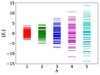
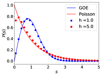
Figure 1: (a) Energy spectrum of random field Heisenberg model for $L=6$ at different disorder strengths. (b) Comparison of the level spacing distribution $\mathcal{P}(s)$ for the random field Heisenberg model. At small disorder ($h=1$), $\mathcal{P}(s)$ follows the GOE distribution, while at larger disorder ($h=5$) it has a Poisson distribution.

We plot representative energy spectra of the Hamiltonian in Fig. 1(a), whose bandwidth increases with disorder strength $h$. More importantly, in all cases, the levels are denser in the middle part of the spectrum, hence the density of state (DOS) is more uniform. For this reason we choose middle part of the spectrum to do level statistics. The evolution of the level spacing distribution at low ($h=1$) and high ($h=5$) disorder strength is shown in Fig. 1(b), which is obtained after implementing the unfolding procedure [57, 58, 59]. We clearly see that at large disorder strength ($h=5$) the level spacing distribution is Poissonian and at small value of disorder ($h=1$) the distribution follows GOE. The fitting for $h=5$ has noticeable deviations around $s\rightarrow 0$ in the finite system, where there remains small but finite correlation between nearby eigenstates. Past studies estimate a critical $h_{c}\approx 3$ [32, 46, 47] for the transition from the thermal phase to the MBL phase.

Recent studies show that even though a machine has no knowledge of level spacing in random matrix theory, a fully-connected feed-forward neural network can, nevertheless, detect the MBL transition in random spin systems, with the raw energy spectra in small systems as training data. However, the large number of parameters in this network makes it difficult to extract “what” machine learns, hence, in this work, we employ the convolutional neural network (CNN) [30] to study the MBL transition.

[] []

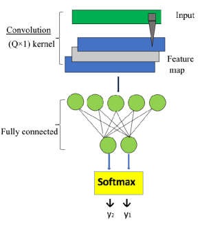
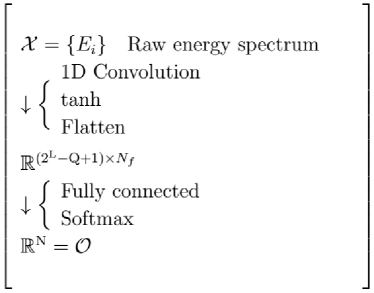
Figure 2: (a) Sketch of the CNN architecture used in the present work. (b) The flow of data in the CNN model.

The CNN model $\mathcal{M}_{\mathrm{CNN}}$ consists of a convolution layer and a fully connected layer as shown Fig. 2(a). In the convolution layer the input data $\mathcal{X}$ is convolved with $N_{f}$ filters $\mathcal{F}^{\beta}$ (also referred as kernel), where $\beta=1,2,\dots,N_{f}$. Mathematically, the 1D convolutions performed by our CNN model can be expressed as,

$$\mathrm{Z}^{\beta}=(\mathcal{X}\ast\mathcal{F}^{\beta})(k)=\sum_{i=1}^{Q}\mathcal{X}(k+i)\mathcal{F}^{\beta}(i),\quad$$ (2)

where $\mathrm{Z}^{\beta}$ is the $\beta$th feature map obtained as the result of the convolution process and $Q$ is the width of the kernel. Filter weights constitute a set of $N_{f}\times Q$ parameters in the convolution layer, which are optimized during the training process. These resulting feature maps are processed by a nonlinear activation function, whose output is flattened and passed to the fully connected layer without pooling. By a linear map with weights $\mathcal{W}$ the flattened output yields $\tilde{y}_{1}$ and $\tilde{y}_{2}$, which correspond to the two phases. The set of weights are also optimized in the training process. Finally, the probability of being in either of the phases is obtained by a softmax function

$$y_{1}^{\mathrm{CNN}} = \frac{\exp(\tilde{y}_{1})}{\exp(\tilde{y}_{1})+\exp(\tilde{y}_{2})}$$ (3)

$$y_{2}^{\mathrm{CNN}} = \frac{\exp(\tilde{y}_{2})}{\exp(\tilde{y}_{1})+\exp(\tilde{y}_{2})}$$ (4)

The flow of the data in the CNN model is summarized in Fig. 2(b).

To classify the thermal and MBL phases, we train the neural network in a supervised learning scheme with a collection of raw eigenvalue spectra obtained via diagonalizing Eq. (1). In other words, we label the spectra with the corresponding phases and train the network to extract relevant features from the input data. In particular, the CNN is trained with the mini-batch gradient descent method. The optimization algorithm searches for an optimal set of parameters that minimizes the cross entropy

$$\mathcal{E}=-\sum_{I=1}^{N_{b}}\sum_{i=1}^{2}y_{I,i}\log y_{I,i}^{\mathrm{CNN}},$$ (5)

where $y_{i}=0$ or $1$ is the true phase label of the $I$th sample, and $N_{b}$ is the size of batch during one training. After the training, the neural network can use its gained knowledge to predict or validate the class for a new set of data. The performance of the network depends on the model of the network, as well as the quality of training. It should be pointed out that, the number of parameters in a CNN is large (although significantly smaller than that of fully-connected NN), hence finding a global minimum of the cross entropy is almost impossible. Nevertheless, our aim is not the precise values of the optimized parameters or the best performance, but a numerical trend in the parameters that enables the machine to extract non-trivial physics.

3 CNN Training Results

We begin by understanding what a CNN learns to distinguish phases, explicitly, the thermal phase at low disorder and the MBL phase at high disorder from energy spectra, as displayed in Fig. 1(a), in the random spin system. We assume no prior knowledge of the exact transition point and numerically generate the raw energy spectrum $\left\{E_{i}\right\}$ of the Heisenberg model deep in each phase. Explicitly, we collect data for the thermal phase (labelled as 0) in the range $1.0\leq h\leq 1.4$, and for the MBL phase (labelled as 1) in the range $4.6\leq h\leq 5.0$. In each region we generate $1000$ samples of $\left\{E_{i}\right\}$ with parameter interval $\Delta h=0.1$. The conventional wisdom is that the energy spectra in the two phases can be distinguished by nearest-neighbour level spacing, as we demonstrate in Fig. 1(b). In the CNN training, we assume we have no knowledge of the level statistics and feed all the labelled data to the CNN for a supervised learning. We then analyze the kernel parameters to gain knowledge on how the neural network filter the energy spectra to distinguish the two phases.

3.1 Filters whose kernel width is 2

An energy spectrum is a 1D set of data, so we use 1D filters with kernel width $Q$. The simplest nontrivial case is $Q=2$. Therefore, we start our training with the CNN architecture that has $2\times 1$ filters, i.e. 1D filters whose kernel width is 2. In the convolution operation the CNN filters extract features from nearest neighbouring levels.

The feature map $\mathrm{Z}^{\beta}$ generated by convolution with a filter $\mathcal{F}^{\beta}=(\mathcal{F}_{1}^{\beta},\mathcal{F}_{2}^{\beta})$ on two neighbouring eigenvalues $E_{i}$ and $E_{i+1}$ is,

$$\mathrm{Z}_{i}^{\beta}=\mathcal{F}_{1}^{\beta}E_{i}+\mathcal{F}_{2}^{\beta}E_{i+1},$$ (6)

where $\beta$ indicates the channel index. For each collection of data we run the training process $\mathcal{T}_{\mathscr{L}}$ $1000$ times. During each $\mathcal{T}_{\mathscr{L}}$, the network parameters are initialized stochastically from a truncated normal distribution having mean $\mu=0$ and standard deviation $\sigma=0.1$. All testing accuracies are close to $100\%$, suggesting that distinguishing the thermal phase from the MBL phase is an easy task for even the simplest CNN architecture.

In Fig. 3(a) we show the resulting filter weights $\mathcal{F}^{\beta}$ from the $1000$ training process, in which we only use $N_{f}=1$ filter. We find that the filter weights split into two branches in quadrants I and III, respectively. We fit the filter weights by

$$\mathcal{F}_{1}^{\beta}=m\mathcal{F}_{2}^{\beta}\pm c,$$ (7)

where the plus sign corresponds to quadrant I and minus to quadrant III. The best fit yields $m=-0.95\pm 0.02$ and $c=0.360\pm 0.003$. We note that $m\approx-1$ so the feature map, according to Eq. (6), is approximately

$$\mathrm{Z}_{i}^{\beta}=\mathcal{F}_{2}^{\beta}\Delta E_{i}\pm 0.36E_{i},$$ (8)

where $\Delta E_{i}=E_{i+1}-E_{i}$ is the nearest-neighbour level spacing. Eq. (8) reveals two underlying features that the neural network filters to distinguish the phases: $\Delta E_{i}$ and $E_{i}$. Because the network identifies the phases with almost perfect accuracy regardless of the value of $\mathcal{F}_{2}^{\beta}$, we conclude that the neural network is not sensitive to level spacing, which is commonly used as a diagnostic for phase transition in disordered and chaotic systems. The apparently surprising result roots in the supervised learning scheme and the disorder strength dependence of the bandwidth. As shown in Fig. 1(a), the bandwidth of the system grows monotonically with the disorder strength. In the supervised learning bandwidth can be a feature that the CNN learns to distinguish phases. For two neighbouring levels we can combine their energies into their difference and mean, which are independent. Our observation suggests that the energy difference is irrelevant, confirming that their mean is the feature that is filtered by the convolution layer to the subsequent fully connected layer, the output of which scales with bandwidth.

[] []

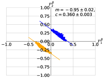
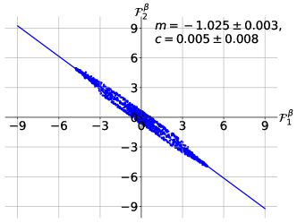
Figure 3: (a) Filter weights after performing convolution with a kernel of width $2$ on the energy spectrum $\{E_{i}\}$ of 10 sites random field Heisenberg chain. Data is shown for $\mathcal{T}_{\mathscr{L}}=1000$ training loops keeping stride $s=1$ and using sigmoid activation function. Other training parameters are: batch size $N_{b}=100$, learning rate $\eta=0.01$, and filter number $N_{f}=1$. (b) Filter weights for all the filter channels obtained from normalized energy levels $\{E_{i}^{\prime}\}$. Other parameters are: $N_{b}=100$, $s=1$, $\eta=0.05$, $N_{f}=3$, and $\mathcal{T}_{\mathscr{L}}=500$. Here we use tanh as the activation function.

This is a vivid example that a machine with a supervised scheme may not always learn nontrivial knowledge. Bandwidth can be used to distinguish a low-disorder system from a high disorder system, but it cannot be used to detect the phase transition point without prior knowledge. The above example is, therefore, a caution to the study of phase transition via deep neural networks.

The failure to gain nontrivial features can be corrected, however, by properly manipulating the input data. We can unbiasedly compare the spectra at various disorder by normalizing the spectrum of a sample by its minimum and maximum energies as

$$E_{i}^{{}^{\prime}}=2\frac{E_{i}-E_{\min}}{E_{\max}-E_{\min}}-1$$ (9)

where $E_{i}^{{}^{\prime}}$ is the normalized energy level. The normalized spectrum $\left\{E_{i}^{{}^{\prime}}\right\}$ always has a bandwidth of 2 and preserves the level statistics of the original spectrum. We then feed the normalized spectrum $\left\{E_{i}^{{}^{\prime}}\right\}$ to the CNN and perform $500$ independent trainings $\mathcal{T}_{\mathscr{L}}$. We find that once the bandwidth effects are removed by normalization the performance of the same neural network drops from $100\%$ to around $70\%$, even though we increase the number of channel to $N_{f}=3$. Fig. 3(b) presents the results of the filter weights $\mathcal{F}^{\beta}$ in all trainings, which fall roughly on a straight line. When we fit the data by

$$\mathcal{F}_{1}^{\beta}=m\mathcal{F}_{2}^{\beta}+c,$$ (10)

we obtain $m=-1.025\pm 0.003$ and $c=0.005\pm 0.008$. The normalization suppresses the intercept to essentially zero, but preserves $m\approx-1$. This means that the convolution layer now only passes the level spacing information to the subsequent layer, consistent with our expectation that level spacing can be used to detect the MBL phase and the MBL-thermal transition.

In Fig. 3(b) we use $N_{f}=3$ convolutional filter channels. The resulting weights for the three channels all prefer level-spacing information, rather than bandwidth. We have also tested training with $N_{f}=1$ and $N_{f}=2$ channels. We find, in general, more training loops (hence longer time) are needed to filter the bandwidth information with less filters. For example, we need about 1000 training loops with $N_{f}=2$, compared to 500 loops with $N_{f}=3$ to obtain a similar trend line as in Fig. 3(b). We speculate that this is because the level spacing distribution is a statistical “order parameter” in this system. Therefore, more level-spacing information can be extracted with a larger $N_{f}$, which allows an easier identification of its distribution.

We also note that the detail of the energy normalization is not important. We also consider the normalization by $E_{i}^{{}^{\prime}}=\left(E_{i}-\overline{E}\right)/\sigma$ where $\overline{E}$ is the average energy of the spectrum and $\sigma$ is the standard deviation from mean value. This normalization convention yields a similar picture for the CNN parameters.

We can attribute the significant drop of the performance of the CNN after we input the normalized spectra to sample-to-sample fluctuations in finite systems. In the conventional level statistics study we identify the phase by analyzing the ensemble averaged level spacing. In the CNN approach, however, we ask which phase each sample belongs to. In a finite system, the fluctuations in energy level spacing, therefore, prevent us from unambiguously classifying individual samples. But over all samples, we still achieve a 70% performance, which is significantly higher than 50% from random guesses. The difference is sufficient for the machine to select the level spacing as the feature map to explore during the convolution. The next question is whether we can boost the performance by increasing the kernel width.

3.2 Filters whose kernel width is 3

The CNN with kernel width 2 extracts the nearest-neighbour level spacing. To extract more information we also study the neural network with filters of kernel width 3, which captures both nearest-neighbour and next-nearest-neighbour level spacings. Explicitly, a filter $\mathcal{F}^{\beta}=(\mathcal{F}_{1}^{\beta},\mathcal{F}_{2}^{\beta},\mathcal{F}_{3}^{\beta})$ yields a feature map in the form

$$\mathrm{Z}_{i}^{\beta}=\mathcal{F}_{1}^{\beta}E_{i}+\mathcal{F}_{2}^{\beta}E_{i+1}+\mathcal{F}_{3}^{\beta}E_{i+2}$$ (11)

Again, we input the energy spectra normalized by their minimum and maximum energies. In this case, we obtain an $82\%$ performance in accuracy among 500 trainings, significantly higher than the 70% with filters of kernel width 2.

We plot the resulting filter weights $\mathcal{F}_{2}^{\beta}$ against $\mathcal{F}_{1}^{\beta}$ in Fig. 4(a) and $\mathcal{F}_{3}^{\beta}$ against $\mathcal{F}_{1}^{\beta}$ in Fig. 4(b) and fit the results by straight lines. We find that

$$\mathcal{F}_{2}^{\beta}=-(0.485\pm 0.005)\mathcal{F}_{1}^{\beta}+(0.01\pm 0.01),$$ (12)

and

$$\mathcal{F}_{3}^{\beta}=(0.85\pm 0.02)\mathcal{F}_{2}^{\beta}+(-0.03\pm 0.03).$$ (13)

The results provide a strong motivation for us to approximate the weights by

$$\mathcal{F}_{2}^{\beta}=-\frac{\mathcal{F}_{1}^{\beta}}{2}\text{\ and\ }\mathcal{F}_{3}^{\beta}=\mathcal{F}_{2}^{\beta},$$ (14)

which lead to the feature map $\mathrm{Z}_{i}^{\beta}$ only in terms of one filter element $\mathcal{F}_{1}^{\beta}$,

$$\mathrm{Z}_{i}^{\beta}\simeq\frac{\mathcal{F}_{1}^{\beta}}{2}(E_{i}-E_{i+1})+\frac{\mathcal{F}_{1}^{\beta}}{2}(E_{i}-E_{i+2})$$ (15)

This feature map is an equal-weight linear combination of the nearest-neighbour and next-nearest-neighbour level spacings.

[] []

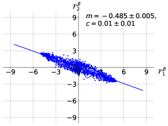
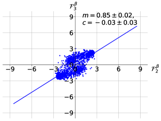
Figure 4: (a) Filter weights $\mathcal{F}_{2}^{\beta}$ as a function of $\mathcal{F}_{1}^{\beta}$ obtained by using a kernel of size $3\times 1$ on normalized energy spectrum $\{E_{i}^{\prime}\}$, the stride is kept to be $\mathrm{s}=1$. Other training parameters are: $N_{b}=100$, $\eta=0.05$, $N_{f}=3$, and $\mathcal{T}_{\mathscr{L}}=500$. (b) Filter weights $\mathcal{F}_{3}^{\beta}$ as a function of $\mathcal{F}_{2}^{\beta}$. Training parameters are the same as in (a).

The filter weights learned by the CNN suggests that the neural network, when given the freedom to choose, tends to use both nearest-neighbour and next-nearest-neighbour level spacings with roughly equal weight to identify the energy spectrum of the two phases across the MBL phase transition. The improved performance confirms that the combination is more effective than using nearest-neighbour level statistics only. Therefore, we will turn to the analysis of the next-nearest-neighbour level statistics in the next subsection and try to understand the machine learning results with kernel width 3.

We note that the training results scatter around the linear regression curve with noticeable deviations. This results from the fact that the neural network has numerous parameters or weights and, therefore, finding the globally optimal, hence reproducible, parameters is almost impossible. However, the goal of our study is not the precision of the parameters, but the numerical trend that allows us to propose alternative level spacings, which may outperform the conventional nearest-neighbour level spacings, at least in finite systems.

3.3 Next-nearest-neighbour level statistics

Before we try to understand the machine learning results, we discuss the distribution of the next-nearest-neighbour level spacings, which is denoted by $\mathcal{P}_{2}(s)$. As for the nearest-neighbour level statistics, we demand

$$\int_{0}^{\infty}\mathcal{P}_{2}(s)ds=\int_{0}^{\infty}s\mathcal{P}_{2}(s)ds=1,$$ (16)

which can be achieved by normalizing the level spacings by their mean.

In the MBL phase neighbouring eigenenergies likely correspond to two wave functions localized in different regions. Therefore, we can write the next-nearest-neighbour level spacing $E_{i+2}-E_{i}=\left(E_{i+2}-E_{i+1}\right)+\left(E_{i+1}-E_{i}\right)$, as the sum of two independent nearest-neighbour level spacings, whose distribution satisfies a Poisson distribution $\mathcal{P}\left(s\right)=\exp\left(-s\right)$. Therefore, we have, for unnormalized level spacing $s^{\prime}$,

$$\tilde{\mathcal{P}}_{2}\left(s^{\prime}\right)\propto\int_{0}^{s^{\prime}}\mathcal{P}\left(s^{\prime}-s_{1}\right)\mathcal{P}\left(s_{1}\right)ds_{1}=s^{\prime}e^{-s^{\prime}}\text{.}$$ (17)

Normalizing the distribution according to Eq. (16), we obtain

$$\mathcal{P}_{2}(s)=4s\exp\left({-2s}\right),$$ (18)

which turns out to be a semi-Poisson distribution. Compared to the nearest-neighbour level statistics, the most noticeable difference is now $\mathcal{P}_{2}\left(0\right)=0$. This is not a manifestation of level repulsion as in the thermal phase; rather, it simply states that three consecutive levels do not coincide.

In the thermal phase neighbouring levels are correlated. In random matrix theory the joint probability density function for eigenvalues is [38]

$$P(\{E_{i}\})\propto\prod_{i<j}|E_{i}-E_{j}|^{\nu}\exp(-A\sum_{i}E_{i}^{2})\text{,}$$ (19)

where $\nu=1$ in the GOE. We show, in A, that the distribution leads to the distribution of next-nearest-neighbour level spacings

$$\mathcal{P}_{2}(s)=\frac{2^{18}}{3^{6}\pi^{3}}s^{4}\exp\left(-\frac{64}{9\pi}s^{2}\right)\text{,}$$ (20)

which is, interestingly, identical to the distribution of nearest-neighbour level spacings in a GSE. In contrast, if we neglect the correlations between neighbouring level spacings and adopt similar derivations as Eq. (17), the distribution of next-nearest-neighbour level spacings is

$$\mathcal{P}_{2}^{{}^{\prime}}\left(s\right)=\pi se^{-\pi s^{2}}+\frac{\pi\left(\pi s^{2}-1\right)}{\sqrt{2}}e^{-\pi s^{2}/2}\text{Erf}\left(\sqrt{\frac{\pi}{2}}s\right)\text{,}$$ (21)

where Erf stands for the error function Erf$\left(z\right)=\frac{2}{\sqrt{\pi}}\int_{0}^{z}e^{-t^{2}}dt$.

In Fig. 5 we plot the distribution of next-nearest-neighbour level spacings of the random spin chains. We confirm that the distribution for $h=1$ agrees well with the GSE distribution, while that for $h=5$ follows the semi-Poisson distribution. For comparison, we also plot Eq. (21) by a black dashed line, which clearly deviates from the data at $h=1$, indicating that the correlation in level spacings is non-negligible.

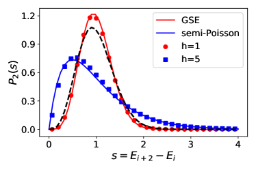
Figure 5: Evolution of next-nearest level spacing distribution from GOE to GSE at $h=1$ and from Poisson to semi-Poisson at $h=5$. The black dashed line corresponds to the distribution in Eq. (21).

Comparing Fig. 5 to Fig. 1(b), we conclude that the distribution of next-nearest-neighbour level spacings can also be used to distinguish the energy spectra in the thermal and MBL phases. Because in the MBL phase the correlation between eigenstates decays exponentially with their distance, it is more advantageous to consider the distribution of next-nearest-neighbour level spacings than that of nearest-neighbour level spacings in finite systems, which, at large disorder, deviates from the Poisson distribution at small level spacings, as shown in Fig. 1(b).

However, the comparison is for the ensemble average. On the other hand, ML tends to ask whether an individual sample belongs to the thermal or the MBL phase, and the phase boundary can be determined by the percentage recognition of the two phases. In this case, our CNN study in the previous subsection reveals roughly equal weights on the two level spacings, which improves the recognition accuracy significantly. We speculate that while the residual level repulsion due to the finite-size effect in the MBL phase favours the next-nearest-neighbour level statistics, the fluctuations in the level spacings tend to blur the difference in the similar peak structures in the two phases. So what we observe is likely a compromise of the two aspects of the finite-size effect. Finally, it’s worth emphasizing the filter size can be further increased to incorporate level spacings on longer ranges, and the higher-order level spacings are also efficient for distinguishing phases. Meanwhile, the results from filter size equals two and three are sufficient to express the main point of current work.

4 Conclusion

We deploy a CNN to study the thermal-MBL transition in a one-dimensional random spin system, using the raw energy spectrum as the training data. Our aim is to reveal the key feature that the neural network extracts to classify the phases. The simplest CNN that contains $2\times 1$ filters can capture the nearest-neighbour level spacings, which can be used to distinguish the thermal phase from the MBL phase. However, the accuracy to identify individual samples is limited by finite-size effect. By using $3\times 1$ filters, the CNN is able to capture next-nearest-neighbouring level spacings. We compare the next-nearest-neighbor level statistics for the thermal and MBL phases to analytical solutions and show that it can also be used to distinguish the two phases. As a result, the CNN improves the test accuracy by $12\%$ by enlarging filters.

Compared to earlier studies, the present approach has the following advantages. First, we use raw energy spectra (normalized to get rid of the trivial band width information in the supervised learning) as the training data. Compared to ES that was used in Ref. [32], our training data is considered to be of “lower level”, which requires less prior knowledge. Second, although the fully-connected NN has been used in learning the thermal-MBL transition[49], the large number of parameters makes it difficult to extract quantities of physical meaning that machine utilizes to distinguish phases. The filters in our CNN architecture allows a clear interpretation of what a machine learns. In contrast, the training with normalized energy spectrum turns out to be much more difficult and unstable for the fully-connected NN. For a comparison, the learning rate in Ref. [49] is the order of $10^{-4}$, which should be reduced to the order of $10^{-8}$ when training data is the normalized energy spectrum. This demonstrates that the NN without a feature extractor is less efficient in learning non-trivial physics, which motivated us to employ a CNN. Finally, we are able to show that machine learning can “discover”less known physical quantity, in this case higher-order level spacings for both the thermal and MBL phases. Therefore, the present work provides a vivid example of how one may use neural networks to develop and to improve methods from low-level data in disordered systems.

In general, our approach can be applied to study dynamical phase transition in any model that has energy or entanglement spectrum. For example, in quantum system with periodic driving where a quasi-energy spectrum replaces the conventional energy spectrum, we believe the CNN can likewise capture the dynamical signal of phase transition through the filters. In addition, by selecting different parts of the energy spectrum as training data, the CNN can also be used to locate the many-body mobility edge.

We note that our discussion only relies on random matrix theory, rather than the specific Hamiltonian. We expect the results can be applied to other disordered and chaotic systems in both ML and conventional studies.

Appendix A Derivation of Eq. (20)

In this appendix we give an analytical derivation for the next-nearest level spacings in thermal phase. We start with the standard (unnormalized) energy level probability density for Gaussian ensembles [38],

$$P\left(\left\{E_{i}\right\}\right)\propto\prod_{i<j}\left|E_{i}-E_{j}\right|^{\nu}e^{-A\sum_{i}E_{i}^{2}}$$ (22)

where $\nu=1$, 2, 4 for GOE, GUE, and GSE, respectively. When dealing with nearest-neighbour level spacing, it is sufficient to consider the $2\times 2$ matrix case [38]. Likewise, to study the next-nearest level spacing, we can consider $3\times 3$ matrix. Introduce $\mathcal{P}_{2}\left(s\right)=P\left(\left|E_{3}-E_{1}\right|=s\right)$, we have

$$\mathcal{P}_{2}\left(s\right)\propto\int_{-\infty}^{\infty}\prod_{i<j}\left|E_{i}-E_{j}\right|^{\nu}\delta\left(s-\left|E_{1}-E_{3}\right|\right)e^{-A\sum_{i}E_{i}^{2}}dE_{1}dE_{2}dE_{3}\text{.}$$ (23)

Now we switch variables to $x_{1}=E_{1}-E_{2}$, $x_{2}=E_{2}-E_{3}$, $x_{3}=\sum_{i=1}^{3}E_{i}$, then

$$\mathcal{P}_{2}\left(s\right) \propto \int_{-\infty}^{\infty}\left|x_{1}\right|^{\nu}\left|x_{2}\right|^{\nu}\left|x_{1}+x_{2}\right|^{\nu}\delta\left(s-\left|x_{1}+x_{2}\right|\right)e^{-\frac{A}{2}\left[x_{1}^{2}+x_{2}^{2}+x_{3}^{2}+\left(x_{1}+x_{2}\right)^{2}\right]}$$ (24)

$$\times\frac{\partial\left(E_{1},E_{2},E_{3}\right)}{\partial\left(x_{1},x_{2},x_{3}\right)}dx_{1}dx_{2}dx_{3}\text{.}$$

In this integral the Jacobian $\frac{\partial\left(E_{1},E_{2},E_{3}\right)}{\partial\left(x_{1},x_{2},x_{3}\right)}$ and the integral for $x_{3}$ are all constants that can be absorbed into the normalization factor. By introducing the polar coordinates $x_{1}=r\cos\theta$, $x_{2}=r\sin\theta$, we can write $\mathcal{P}_{2}\left(s\right)$ as

$$\mathcal{P}_{2}\left(s\right) \propto \int_{0}^{\infty}\int_{0}^{2\pi}r^{3\nu}\left|\cos\theta\right|^{\nu}\left|\sin\theta\right|^{\nu}\left|\cos\theta+\sin\theta\right|^{\nu}$$ (25)

$$\times\delta\left(s-r\left|\cos\theta+\sin\theta\right|\right)e^{-\frac{A}{2}r^{2}\left(2+\sin 2\theta\right)}rdrd\theta$$

$$= \int_{0}^{2\pi}\left(\frac{s}{\left|\cos\theta+\sin\theta\right|}\right)^{3\nu+1}e^{-\frac{A\left(2+\sin 2\theta\right)}{2\left|\cos\theta+\sin\theta\right|^{2}}s^{2}}$$

$$\times\left|\cos\theta\right|^{\nu}\left|\sin\theta\right|^{\nu}\left|\cos\theta+\sin\theta\right|^{\nu}d\theta\text{.}$$

Although the integral for $\theta$ is difficult to solve, it only contributes to the normalization factor and does not influence the scaling behavior of $s$. Therefore, we can simplify $\mathcal{P}_{2}\left(s\right)$ to

$$\mathcal{P}_{2}\left(s\right)=C\left(\nu\right)s^{3\nu+1}e^{-A\left(\nu\right)s^{2}}\text{.}$$ (26)

For GOE, we have $\nu=1$. Finally, by imposing the normalization condition

$$\int_{0}^{\infty}\mathcal{P}_{2}\left(s\right)ds=1\text{, }\int_{0}^{\infty}s\mathcal{P}_{2}\left(s\right)=1$$ (27)

we can determine the coefficients $C\left(\nu\right)$ and $A\left(\nu\right)$ and obtain the GSE distribution as in Eq. (20). The higher-order level spacing distributions can be derived in a similar manner.

References

References

- [1] I. V. Gornyi, A. D. Mirlin, and D. G. Polyakov, Phys. Rev. Lett. 95, 206603 (2005); 95, 046404 (2005).
- [2] D. M. Basko, I. L. Aleiner, and B. L. Altshuler, Ann. Phys. 321, 1126 (2006).
- [3] H. Li and F. D. M. Haldane, Phys. Rev. Lett. 101 , 010504 (2008).
- [4] J. H. Bardarson, F. Pollmann, and J. E. Moore, Phys. Rev. Lett. 109, 017202 (2012).
- [5] J. A. Kjall, J. H. Bardarson, and F. Pollmann, Phys. Rev. Lett. 113, 107204 (2014).
- [6] S. D. Geraedts, R. Nandkishore, and N. Regnault, Phys. Rev. B 93, 174202 (2016).
- [7] S. D. Geraedts, N. Regnault, and R. M. Nandkishore, New J. Phys. 19, 113921 (2017).
- [8] X. Yu, D. J. Luitz, and B. K. Clark, Phys. Rev. B 94, 184202 (2016).
- [9] Z.-C. Yang, C. Chamon, A. Hamma, and E. R. Mucciolo, Phys. Rev. Lett. 115, 267206 (2015).
- [10] M. Serbyn, A. A. Michailidis, M. A. Abanin, and Z. Papic, Phys. Rev. Lett. 117, 160601 (2016).
- [11] J. Gray, S. Bose, and A. Bayat, Phys. Rev. B 97, 201105 (2018).
- [12] X. Li, S. Ganeshan, J. H. Pixley, and S. Das Sarma, Phys. Rev. Lett. 115, 186601 (2015).
- [13] M. Serbyn, Z. Papic, and D. A. Abanin, Phys. Rev. X 5, 041047 (2015).
- [14] I. Goodfellow, Y. Bengio, and A. Courville, Deep Learning (MIT Press 2016).
- [15] A. Tanaka and A. Tomiya, J. Phys. Soc. Jpn. 86, 063001 (2017).
- [16] J. Carrasquilla and R. G. Melko, Nat. Phys. 13, 431 (2017).
- [17] G. Torlai and R. G. Melko, Phys. Rev. B 94, 165134 (2016).
- [18] Y. Zhang and E.-A. Kim, Phys. Rev. Lett. 118, 216401 (2017).
- [19] Y. Zhang, R. G. Melko, and E.-A. Kim, Phys. Rev. B 96, 245119 (2017).
- [20] Y.-H. Liu and E. P. L. van Nieuwenburg, Phys. Rev. Lett. 120, 176401 (2018).
- [21] L. Wang, Phys. Rev. B 94, 195105 (2016).
- [22] K. Ch’ng, J. Carrasquilla, R. G. Melko, and E. Khatami, Phys. Rev. X 7, 031038 (2017).
- [23] A. Morningstar and R. G. Melko, J. Mach. Learn. Res. 18, 5975 (2018).
- [24] P. Ponte and R. G. Melko, Phys. Rev. B 96, 205146 (2017).
- [25] C.-D. Li, D.-R. Tan, and F.-J. Jiang, Ann. Phys. 391 , 312-331 (2018).
- [26] T. Ohtsuki and T. Ohtsuki, J. Phys. Soc. Jpn. 85 , 123706 (2016); 86, 044708 (2017).
- [27] W. Hu, R. R. P. Singh, and R. T. Scalettar, Phys. Rev. E 95, 062122 (2017).
- [28] Z. Li, M. Luo, and X. Wan, Phys. Rev. B 99, 075418 (2019).
- [29] W.-J. Rao, Z. Li, Q. Zhu, M. Luo, and X. Wan, Phys. Rev. B 97, 094207 (2018).
- [30] A. Tanaka and A. Tomiya, J. Phys. Soc. Jpn. 86, 063001 (2017).
- [31] E. Khatami, E. Guardado-Sanchez, B. M. Spar, J. F. Carrasquilla, W. S. Bakr, and R, T. Scalettar, arXiv:2002.12310.
- [32] E. P. L. van Nieuwenburg, Y.-H Liu, and S. D. Huber, Nat. Phys. 13, 435 (2017).
- [33] E. van Nieuwenburg, E. Bairey, and G. Refael, Phys. Rev. B 98, 060301 (2018).
- [34] J. Venderley, V. Khemani, and E.-A. Kim, Phys. Rev. Lett. 120, 257204 (2018).
- [35] F. Schindler, N. Regnault, and T. Neupert, Phys. Rev. B 95, 245134 (2017).
- [36] Y.-T. Hsu, X. Li, D.-L. Deng, and S. Das Sarma, Phys. Rev. Lett. 121, 245701 (2018).
- [37] E. V. H. Doggen, F. Schindler, K. S. Tikhonov, A. D. Mirlin, T. Neupert, D. G. Polyakov, and I. V. Gornyi, Phys. Rev. B 98, 174202 (2018).
- [38] F. Haake, Quantum Signatures of Chaos (Springer 2001).
- [39] E. P. Wigner, Ann. Phys. (N.Y.) 53,36 (1951); 62, 548 (1955); 67, 325 (1958).
- [40] F. J. Dyson, J. Math. Phys. 3, 140 (1962).
- [41] F. J. Dyson, J. Math. Phys. 3, 1191 (1962).
- [42] A. Pal and D. A. Huse, Phys. Rev. B 82, 174411 (2010).
- [43] S. Johri, R. Nandkishore, and R. N. Bhatt, Phys. Rev. Lett. 114, 117401 (2015).
- [44] D. J. Luitz, N. Laflorencie, and F. Alet, Phys. Rev. B 91, 081103(R) (2015).
- [45] M. Serbyn and J. E. Moore, Phys. Rev. B 93, 041424(R) (2016).
- [46] N. Regnault and R. Nandkishore, Phys. Rev. B 93, 104203 (2016).
- [47] N. Regnault and R. Nandkishore, Phys. Rev. B 93, 104203 (2016).
- [48] J. M. G. Gomez, R. A. Molina, A. Relano, and J. Retamosa, Phys. Rev. E 66, 036209 (2002).
- [49] W.-J. Rao, J. Phys.:Condens. Matter 30, 395902 (2018).
- [50] F. Alet and N. Laflorencie, arXiv:1711.03145 (2018).
- [51] E. Hofstetter and M. Schreiber, Phys. Rev. B 48, 16979 (1993).
- [52] A. D. Mirlin, Statistics of energy levels and eigenfunctions in disordered systems, Physics Reports 326, 259 (2000).
- [53] B. I. Shklovskii, B. Shapiro, B. R. Sears, P. Lambrianides, and H. B. Shore, Phys. Rev. Lett. 47 11487 (1993).
- [54] Y. Avishai, J. Richert, and R. Berkovits, Phys. Rev. B 66, 052416 (2002).
- [55] O. Bohigas, M. J. Giannoni, and C. Schmit, Phys. Rev. Lett. 52, 1 (1984).
- [56] J. X. Zhong and T. Geisel, Phys. Rev. E 59, 4071 (1999).
- [57] K. Kudo and T. Deguchi, Phys. Rev. B 69, 132404 (2004).
- [58] L. F. Santos and E. J. Torres-Herrera, Nonequilibrium quantum dynamics of many-body systems, in Chaotic, Fractional, and Complex Dynamics: New Insights and Perspectives, (Springer), (2018).
- [59] A. Gubin and L. F. Santos, Am. J. Phys, 95, 246 (2012).