Automotive-Radar-Based 50-cm Urban Positioning

Abstract

Deployment of automated ground vehicles (AGVs) beyond the confines of sunny and dry climes will require sub-lane-level positioning techniques based on radio waves rather than near-visible-light radiation. Like human sight, lidar and cameras perform poorly in low-visibility conditions. This paper develops and demonstrates a novel technique for robust 50-cm-accurate urban ground positioning based on commercially-available low-cost automotive radars. The technique is computationally efficient yet obtains a globally-optimal translation and heading solution, avoiding local minima caused by repeating patterns in the urban radar environment. Performance is evaluated on an extensive and realistic urban data set. Comparison against ground truth shows that, when coupled with stable short-term odometry, the technique maintains $95$-percentile errors below $50\text{\,}\mathrm{cm}$ in horizontal position and $1\mathrm{°}$ in heading.

I Introduction

Development of automated ground vehicles (AGVs) has spurred research in lane-keeping assist systems, automated intersection management [1], tight-formation platooning, and cooperative sensing [2, 3], all of which demand accurate (e.g., 50-cm at 95%) ground vehicle positioning in an urban environment. But the majority of positioning techniques developed thus far depend on lidar or cameras, which perform poorly in low-visibility conditions such as snowy whiteout, dense fog, or heavy rain. Adoption of AGVs in many parts of the world will require all-weather localization techniques.

Radio-wave-based sensing techniques such as radar and GNSS (global navigation satellite system) remain operable even in extreme weather conditions [4] because their longer-wavelength electromagnetic radiation penetrates snow, fog, and rain. Carrier-phase-differential GNSS (CDGNSS) has been successfully applied for the past two decades as an all-weather decimeter-accurate localization technique in open-sky conditions. Coupling a CDGNSS receiver with a tactical-grade inertial sensor, as in [5, 6, 7, 8] delivers robust high-accuracy positioning even during the extended signal outages common in the urban environment, but such systems are far too expensive for widespread deployment on AGVs. Recent work has shown that 20-cm-accurate (95%) CDGNSS positioning is possible at low cost even in dense urban areas, but solution availability remains below 90%, with occasional long gaps between high-accuracy solutions [9]. Moreover, the global trend of increasing radio interference in the GNSS bands, whether accidental or deliberate [10], underscores the need for GNSS-independent localization: GNSS jamming cannot be allowed to paralyze an area’s automated vehicle networks.

Clearly, there is a need for AGV localization that is low cost, accurate at the $\approx$$50$-cm level, robust to low-visibility conditions, and continuously available. This paper is the first to establish that automotive-radar-based localization can meet these criteria.

Mass-market commercialization has brought the cost of automotive radar down enough that virtually all current production vehicles are equipped with at least one radar unit, which serves as the primary sensor for adaptive cruise control and automatic emergency braking. But use of automotive radar for localization faces the significant challenges of data sparsity and noise: an automotive radar scan has vastly lower resolution than a camera image or a dense lidar scan, and is subject to high rates of false detection (clutter) and missed detection. As such, it is nearly impossible to deduce semantic information or to extract distinctive environmental features from an individual radar scan. This is clear from Fig. 1, which shows a sparse smattering of reflections from a single composite scan using three radar units. The key to localization is to aggregate sequential scans into a batch, as in Fig. 1, where environmental structure is clearly evident. Even still, the data remain so sparse that localization based on traditional machine vision feature extraction and matching is not promising.

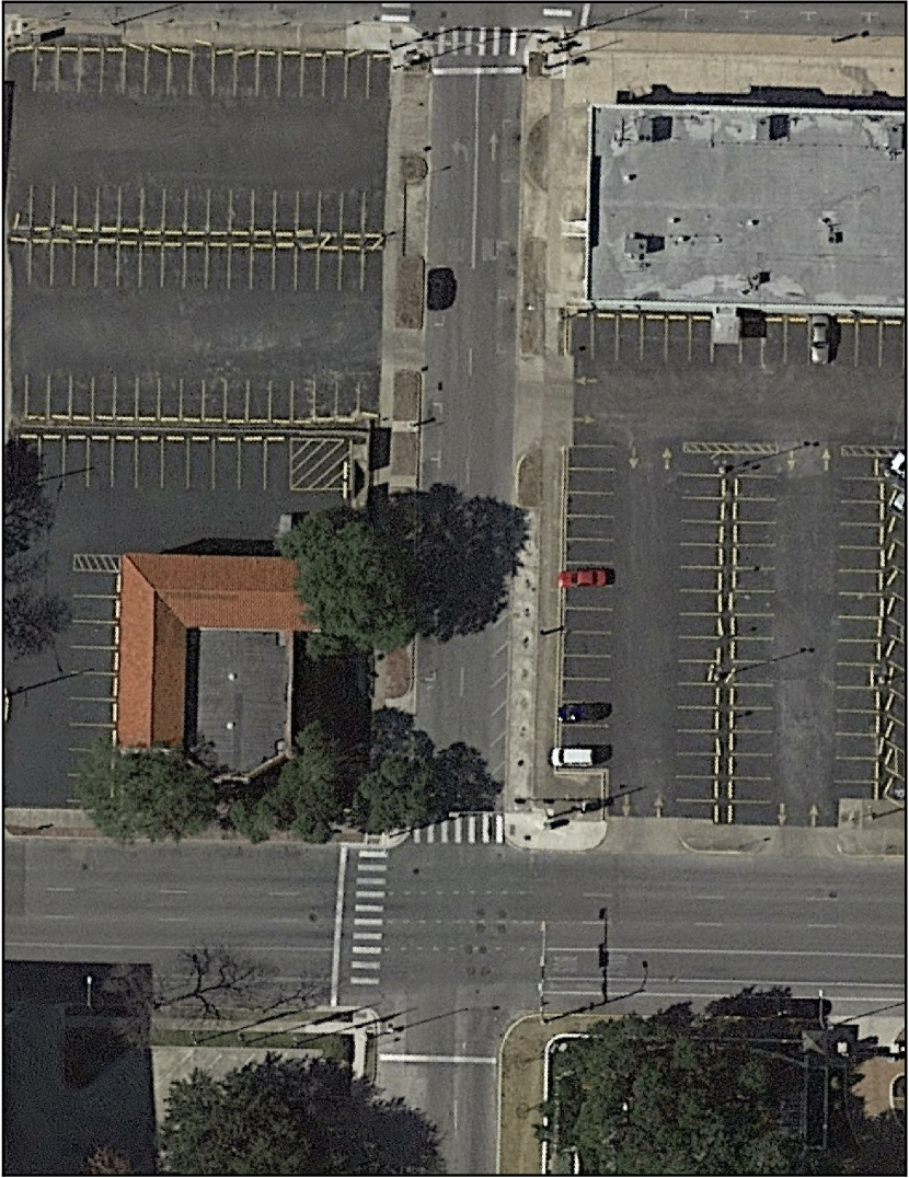
(a)

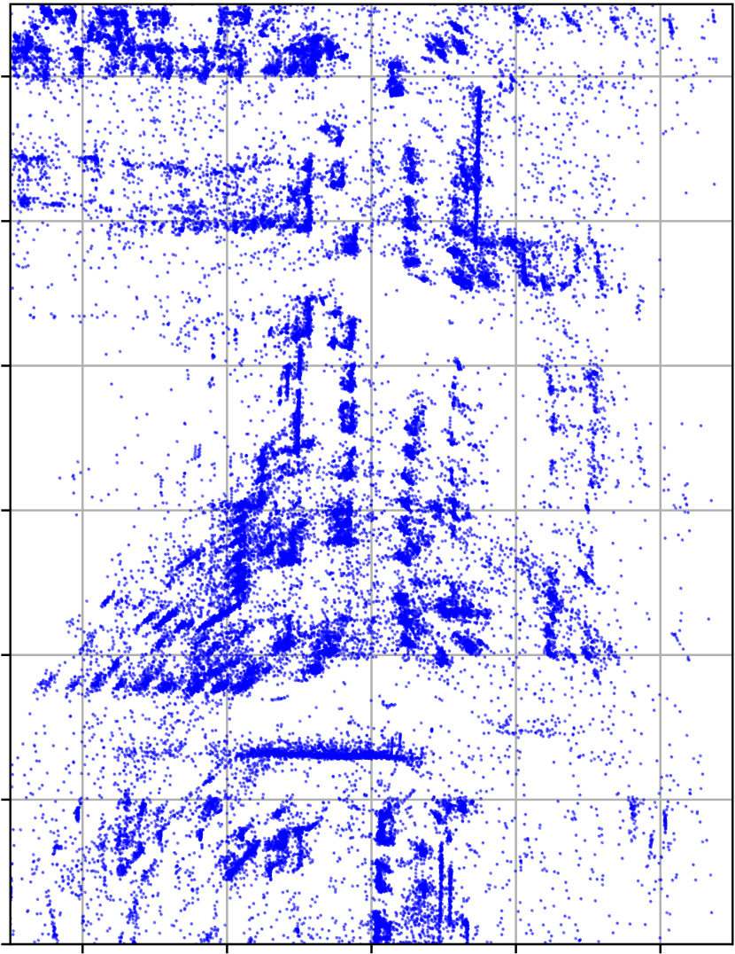
(b)

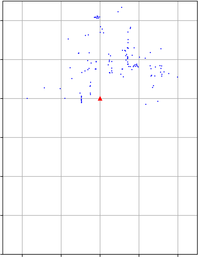
(c)

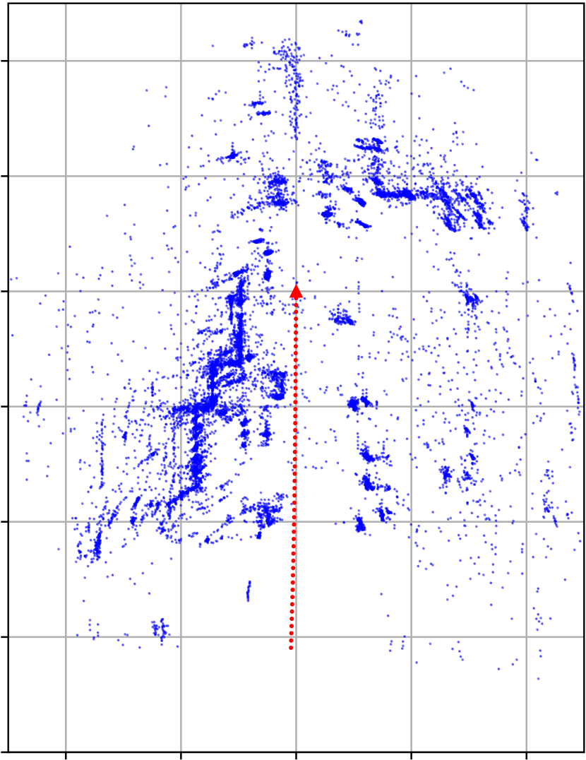
(d)

Figure 1: Panel (a) shows a satellite view of the environment being mapped with automotive radar. Panel (b) shows the generated radar map point cloud with vehicle pose obtained from a reference localization system. Note the repeating structure along the road side due to parked vehicles. An individual radar scan obtained during localization is shown in panel (c), along with the red triangle denoting vehicle location and heading. The scan is sparse and contains significant clutter, making it challenging to register to the prior map. Panel (d) shows a batch of radar scans during localization, with the red dots denoting the vehicle trajectory over the past five seconds. The batch captures the underlying structure which can be registered to the prior map.

This paper proposes a two-step process for radar-based localization. The first is the mapping step: creation of a geo-referenced two-dimensional aggregated map of all radar targets across an area of interest. Fig. 1 shows such a map, hereafter referred to as a radar map. The full radar map used throughout this paper, of which Fig. 1 is a part, was constructed with the benefit of a highly stable inertial platform so that a trustworthy ground truth map would be available against which maps generated by other techniques could be compared. But an expensive inertial system or dedicated mobile mapping vehicle is not required to create a radar map. Instead, it can be crowd-sourced from the very user vehicles that will ultimately exploit the map for localization. During periods of favorable lighting conditions and good visibility, user vehicles can exploit a combination of low-cost CDGNSS, as in [9], and GNSS-aided visual simultaneous localization and mapping, as in [11], to achieve the continuous decimeter-and-sub-degree-accurate geo-referenced position and orientation (pose) required to lay down an accurate radar map. In other words, the radar map can be created when visibility is good and then exploited at any later time, such as during times of poor visibility.

Despite aggregation over multiple vehicle passes, the sparse and cluttered nature of automotive radar data is evident from the radar map shown in Fig. 1: the generated point cloud is much less dense and has a substantially higher fraction of spurious returns than a typical lidar-derived point cloud, making automotive-radar-based localization a significantly more challenging problem.

The second step of this paper’s technique is the localization step. Using some type of all-weather odometric technique such as inertial sensing, radar odometry, or wheel rotation and steering encoders—or a combination of these—the estimated changes in vehicle pose over a short interval (e.g., $5\text{\,}\mathrm{s}$) are used to spatially organize the multiple radar scans over the interval and generate what is hereafter referred to as a batch of scans, or batch for short. Fig. 1 shows a five-second batch terminating at the same location as the individual scan in Fig. 1. In contrast to the individual scan, some environmental structure emerges in the batch of scans, making robust registration to the map feasible. Even so, the localization problem remains challenging due to the dynamic radar environment: note the absence of parked cars on the left side of the street during localization.

Contributions. This paper develops a robust computationally efficient correlation-maximization-based globally-optimal radar scan registration algorithm that estimates a two-dimensional translational and a one-dimensional rotational offset between a prior radar map and a batch of current scans. Significantly, the technique can be applied to the highly sparse and cluttered data produced by commercially-available low-cost automotive radars. Maximization of correlation is shown to be equivalent to minimization of the $L^{2}$ distance between the prior map and the batch probability hypothesis densities.

The proposed method relies on the generation of a batch of radar scans using odometric sensors over short time intervals. An important contribution of this work is to analyze the robustness of the proposed method to short batch lengths and odometric imperfections.

This paper also presents the first evaluation of low-cost automotive-grade radar-based urban positioning on the large-scale dataset described in [12]. Data from automotive sensors are collected over two $1.5\text{\,}\mathrm{h}$ driving sessions through the urban center of Austin, TX on two separate days specifically chosen to provide variety in traffic and parking patterns. Comparison with a post-processed ground truth trajectory shows that proposed radar-based localization algorithm has $95$-percentile errors of $44\text{\,}\mathrm{cm}$ in horizontal position and $0.59\mathrm{°}$ in heading when using drift-free $5\text{\,}\mathrm{s}$ batches.

Organization of the rest of this paper. Sec. II describes the theoretical underpinnings of the proposed localization technique and explains its modeling assumptions. Sec. III compares and contrasts the proposed approach with the prior work in related fields. Implementation details concerning computational efficiency and low-cost automotive radar sensor modeling are presented in Sec. IV. Experimental results on field data are detailed and evaluated in Sec. V, and Sec. VI gives concluding remarks.

II Localization Technique

This section describes the theoretical formulation of the localization technique adopted in this paper. It first details the statistical motivation behind the method, and then develops an efficient approximation to the exact solution.

II-A Localization using Probability Hypothesis Density

For the purpose of radar-based localization, an AGVs environment can be described as a collection of arbitrarily shaped radar reflectors in a specific spatial arrangement. Assuming sufficient temporal permanence of this environment, radar-equipped AGVs make sample measurements of the underlying structure over time.

II-A1 The Probability Hypothesis Density Function

A probabilistic description of the radar environment is required to set up radar-based localization as an optimization problem. This paper chooses the probability hypothesis density (PHD) function [13] representation of the radar environment. The PHD at a given location gives the density of the expected number of radar reflectors at that location. For a static radar environment, the PHD $D(\bm{x})$ at a location $\bm{x}\in\mathcal{X}$ can be written as

$$D(\bm{x})=I\cdot p(\bm{x})$$

where $\mathcal{X}$ is the set of all locations in the environment, $p(\bm{x})$ is a probability density function such that $\int p(\bm{x}){\rm d}\bm{x}=1$, and $I$, the intensity, is the total number of radar reflectors in the environment. For a time-varying radar environment, both $I$ and $p(\bm{x})$ are functions of time. For $\mathcal{A}\subset\mathcal{X}$, the expected number of radar reflectors in $\mathcal{A}$ is given as

$$I_{\mathcal{A}}=\int_{\mathcal{A}}D(\bm{x}){\rm d}\bm{x}$$

II-A2 Estimating Vehicle State from PHDs

Let $D_{\rm m}(\bm{x})$ denote the “map” PHD function representing the distribution of radar reflectors in an environment, estimated as a result of mapping with known vehicle poses. During localization, the vehicle makes a radar scan, or a series of consecutive radar scans. A natural solution to the vehicle localization problem may be stated as the vehicle pose which maximizes the likelihood of the observed batch of scans, given that the scan was drawn from $D_{\rm m}(\bm{x})$ [14]. This maximum likelihood estimate (MLE) has many desirable properties such as asymptotic efficiency. However, the MLE solution is known to be sensitive to outliers that may occur if the batch of scans was sampled from a slightly different PHD, e.g., due to variations in the radar environment between mapping and localization [15].

A more robust solution to the PHD-based localization problem may be stated as follows. Let $\bm{\Theta}$ denote the vector of parameters of the rigid or non-rigid transformation $\mathcal{T}$ between the vehicle’s prior belief of its pose, and its true pose. For example, in case of a two-dimensional rigid transformation, $\bm{\Theta}={\mathopen{}\mathclose{{}\left[\Delta x,\Delta y,\Delta\phi}\right]}^{\top}$, where $\Delta x$ and $\Delta y$ denote a two-dimensional position and $\Delta\phi$ denotes heading. Also, let $D_{\rm b}(\bm{x}^{\prime})$ denote a local “batch” PHD function estimated from a batch of scans during localization, defined over $\bm{x}^{\prime}\in\mathcal{A}\subset\mathcal{X}$. This PHD is represented in the coordinate system consistent with vehicle’s prior belief, such that $\bm{x}^{\prime}=\mathcal{T}_{\bm{\Theta}}(\bm{x})$. Estimating the vehicle pose during localization is defined as estimating $\bm{\Theta}$ such that some distance metric between the PHDs $D_{\rm m}(\bm{x})$ and $D_{\rm b}(\bm{x}^{\prime})$ is minimized.

This paper chooses the $L^{2}$ distance between $D_{\rm m}(\bm{x})$ and $D_{\rm f}(\bm{x}^{\prime})$ as the distance metric to be minimized. As compared to the MLE which minimizes Kullback-Leibler divergence, $L^{2}$ minimization trades off asymptotic efficiency for robustness to measurement model inaccuracy [15]. The $L^{2}$ distance $d_{L^{2}}(\bm{\Theta})$ to be minimized is given as

$$d_{L^{2}}(\bm{\Theta})=\int_{\mathcal{A}}{\mathopen{}\mathclose{{}\left(D_{\rm m}(\bm{x})-D_{\rm b}(\mathcal{T}_{\bm{\Theta}}(\bm{x}))}\right)}^{2}{\rm d}\bm{x}$$

For rigid two-dimensional transformations, it can be shown as follows that minimizing the $L^{2}$ distance between the PHDs is equivalent to maximization of the cross-correlation between the PHDs.

$$\widehat{\bm{\Theta}} =\operatorname*{\arg\!\min}_{\bm{\Theta}^{\prime}}\int_{\mathcal{A}}{\mathopen{}\mathclose{{}\left(D_{\rm m}(\bm{x})-D_{\rm b}(\mathcal{T}_{\bm{\Theta}^{\prime}}(\bm{x}))}\right)}^{2}{\rm d}\bm{x}$$

$$\begin{multlined}=\operatorname*{\arg\!\min}_{\bm{\Theta}^{\prime}}\mathopen{}\mathclose{{}\left[\int_{\mathcal{A}}D_{\rm m}^{2}(\bm{x}){\rm d}\bm{x}+\int_{\mathcal{A}}D_{\rm b}^{2}(\mathcal{T}_{\bm{\Theta}^{\prime}}(\bm{x})){\rm d}\bm{x}}\right.\\ \mathopen{}\mathclose{{}\left.-2\int_{\mathcal{A}}D_{\rm m}(\bm{x})D_{\rm b}(\mathcal{T}_{\bm{\Theta}^{\prime}}(\bm{x})){\rm d}\bm{x}}\right]\end{multlined}=\operatorname*{\arg\!\min}_{\bm{\Theta}^{\prime}}\mathopen{}\mathclose{{}\left[\int_{\mathcal{A}}D_{\rm m}^{2}(\bm{x}){\rm d}\bm{x}+\int_{\mathcal{A}}D_{\rm b}^{2}(\mathcal{T}_{\bm{\Theta}^{\prime}}(\bm{x})){\rm d}\bm{x}}\right.\\ \mathopen{}\mathclose{{}\left.-2\int_{\mathcal{A}}D_{\rm m}(\bm{x})D_{\rm b}(\mathcal{T}_{\bm{\Theta}^{\prime}}(\bm{x})){\rm d}\bm{x}}\right]$$

Note that the first term above is fixed during optimization, while the second term is invariant under rigid transformation. As a result, the above optimization is equivalent to maximizing the cross-correlation:

$$\widehat{\bm{\Theta}}=\operatorname*{\arg\!\max}_{\bm{\Theta}^{\prime}}\int_{\mathcal{A}}D_{\rm m}(\bm{x})D_{\rm b}(\mathcal{T}_{\bm{\Theta}^{\prime}}(\bm{x})){\rm d}\bm{x}$$ (1)

For differentiable $D_{\rm m}$ and $D_{\rm b}$, the above optimization can be solved with gradient-based methods. However, as detailed in Sec. III, the cross-correlation maximization problem in the urban AGV environment may have locally optimal solutions in the vicinity of the global minimum due to repetitive structure of radar reflectors. In applications with high integrity requirements, a search for the globally optimal solution is necessary. This paper notes that if the PHDs in (1) were to be discretized in $\bm{x}$, then the cross-correlation values can be evaluated exhaustively with computationally efficient techniques. Let $\bm{x}_{pq}$ denote the location at the $(p,q)$ translational offset in discretized $\mathcal{A}$. Then

$$\widehat{\bm{\Theta}}=\operatorname*{\arg\!\max}_{\bm{\Theta}^{\prime}}\sum_{p=0}^{P-1}\sum_{q=0}^{Q-1}D_{\rm m}(\bm{x}_{pq})D_{\rm b}(\lfloor\mathcal{T}_{\bm{\Theta}^{\prime}}(\bm{x}_{pq})\rceil)$$ (2)

where $\lfloor.\rceil$ denotes the nearest grid point in the discretized space.

The technique developed above relies on the PHDs $D_{\rm m}$ and $D_{\rm b}$. The next subsections detail the recipe for estimating these PHDs from the radar observations.

II-B Estimating the map PHD from measurements

This section addresses the procedure to estimate the map PHD $D_{\rm m}(\bm{x})$ from radar measurements. This paper works with an occupancy grid map (OGM) approximation to the continuous PHD function. In [16], it has been shown that the PHD representation is a limiting case of the OGM as the grid cell size becomes vanishingly small. Intuitively, let $c_{pq}$ denote the grid cell region with center $\bm{x}_{pq}$, and let $\delta c_{pq}$ denote the area of this grid cell, which is small enough such that no more than one reflector may be found in any cell. Let $p_{pq}(O)$ denote the occupancy probability of $c_{pq}$, and let $\mathcal{A}$ be defined as the region formed by the union of all $c_{pq}$ whose centers $\bm{x}_{pq}$ fall within $\mathcal{A}$. Then, the expected number of radar reflectors $\mathbb{E}\mathopen{}\mathclose{{}\left[\mathopen{}\mathclose{{}\left|{\mathcal{A}}}\right|}\right]$ in $\mathcal{A}$ is given by

$$\mathbb{E}\mathopen{}\mathclose{{}\left[|\mathcal{A}|}\right]=\sum_{c_{pq}\in\mathcal{A}}p_{pq}(O) =\sum_{c_{pq}\in\mathcal{A}}\frac{p_{pq}(O)}{\delta c_{pq}}\delta c_{pq}$$

$$\triangleq\sum_{c_{pq}\in\mathcal{A}}\bar{D}(\bm{x}_{pq})\delta c_{pq}$$

$$=\int_{\mathcal{A}}\bar{D}(\bm{x}_{pq}){\rm d}\bm{x},\quad{\rm as}~{}\lim_{\delta c_{pq}\rightarrow 0}$$

where $\bar{D}(\bm{x}_{pq})\triangleq\frac{p_{pq}(O)}{\delta c_{pq}}$ can be considered to be an approximation of the PHD $D(\bm{x})$ for $\bm{x}\in c_{pq}$ since its integral over $\mathcal{A}$ is equal to the expected number of reflectors in $\mathcal{A}$.

The advantage of working with an OGM approximation of the PHD is two-fold: first, since the OGM does not attempt to model individual objects, it is straightforward to represent arbitrarily-shaped objects, and second, in contrast to the “point target” measurement model assumption in standard PHD filtering, the OGM can straightforwardly model occlusions due to extended objects.

At this point, the task of estimating $D_{\rm m}(\bm{x})$ has been reduced to estimating the occupancy probability of each grid cell in discretized $\mathcal{A}$. Each grid cell $c_{pq}$ takes up one of two states: occupied ($O$) or free ($F$). Based on the radar measurement $\bm{z}_{k}$ at each time $k$, the Bernoulli probability distribution of such binary state cells may be recursively updated with the binary Bayes filter. In particular, let $\bm{z}_{1:k}$ denote all radar measurements made up to time $k$, and let

$$l_{pq}^{k}(O)\triangleq\log{\frac{p_{pq}(O~{}|~{}\bm{z}_{1:k})}{1-p_{pq}(O~{}|~{}\bm{z}_{1:k})}}$$ (3)

denote the log odds ratio of $c_{pq}$ being in state $O$. Also define $l_{pq}^{0}(O)$ as

$$l_{pq}^{0}(O)\triangleq\log{\frac{p_{pq}(O)}{1-p_{pq}(O)}}$$

with $p_{pq}(O)$ being the prior belief on the occupancy state of $c_{pq}$ before any measurements are made. With these definitions, the binary Bayes filter update is given by [17]

$$l_{pq}^{k}(O)=\log{\frac{p_{pq}(O~{}|~{}\bm{z}_{k})}{1-p_{pq}(O~{}|~{}\bm{z}_{k})}}-l_{pq}^{0}(O)+l_{pq}^{k-1}(O)$$ (4)

where $p_{pq}(O~{}|~{}\bm{z}_{k})$ is known as the inverse sensor model: it describes the probability of $c_{pq}$ being in state $O$, given only the latest radar scan $\bm{z}_{k}$.

The required occupancy probability $p_{pq}(O~{}|~{}\bm{z}_{1:k})$ is easy to compute from the log odds ratio in (3). Observe that the inverse sensor model $p_{pq}(O~{}|~{}\bm{z}_{k})$, in addition to the prior occupancy belief $p_{pq}(O)$, completely describes the procedure for estimating the OGM from radar measurements, and hence approximating the PHD. Adapting $p_{pq}(O~{}|~{}\bm{z}_{k})$ to the characteristics of the automotive radar sensors, however, is not straightforward, and will be the topic of Sec. IV-B.

II-C Estimating the batch PHD from measurements

The procedure for generating an approximation to $D_{\rm b}(\bm{x}^{\prime})$ from a batch of radar measurements is identical to the procedure for generating $D_{\rm m}(\bm{x})$ from mapping vehicle data, except that precise, absolute location and orientation data is not available during localization. Instead, inertial odometry is used to estimate the relative locations and orientations of each radar scan in the batch, and the scans are transformed into a common coordinate frame before updating the occupancy state of grid cells.

Once the map and batch PHDs have been approximated from radar measurements, the correlation-maximization technique developed in Sec. II-A can be applied to find a solution to the localization problem.

III Related Work

This section reviews various techniques which may be applicable to the radar-based mapping and localization problem. These include work on point cloud alignment and image registration techniques, occupancy grid-based mapping and localization, and random-finite-set-based mapping and localization.

Related work in point cloud alignment. A radar-based map can have many different representations. One obvious representation is to store all the radar measurements as a point cloud. Fig. 1 is an example of this representation. Localization within this map can be performed with point cloud registration techniques like the iterative closest point (ICP) algorithm. ICP is known to converge to local minima which may occur due to outlying points that do not have correspondences in the two point clouds being aligned. A number of variations and generalizations of ICP robust to such outliers have been proposed in the literature [18, 19, 20, 15, 14, 21].

However, automotive radar data in urban areas exhibit another source of incorrect-but-plausible registration solutions which are not addressed in the above literature—repetitive structure, e.g., due to a series of parked cars, may result in multiple locally-optimal solutions within $23\text{\,}\mathrm{m}$ of the globally-optimal solution. Gradient-based techniques which iteratively estimate correspondences based on the distance between pairs of points are susceptible to converge to such locally-optimal solutions. To demonstrate this phenomenon, the coherent point drift algorithm (CPD) [14], a robust generalization of ICP, is applied to align the map and batch point cloud data collected as part of this work. Fig. 2 shows an example of incorrect convergence for CPD. Observe that the map point cloud in Fig. 2, shown in blue, has four dominant parallel features: a row of parked cars flanked by a building front on each side of the street. In this scenario, when aligning a $5\text{\,}\mathrm{s}$ batch of radar scans shown in red, the CPD algorithm converges to a locally-optimal solution where two of the four parallel features line up correctly. This solution is about $4\text{\,}\mathrm{m}$ south of the globally-optimal solution.

Figure 2: The radar map point cloud is shown in blue and a $5\text{\,}\mathrm{s}$ batch of radar scans is shown in red. Note that the map point cloud has four dominant parallel features: a row of parked cars flanked by a building front on each side of the street. The two point clouds are aligned with the CPD algorithm until convergence. Note the offset of the two point clouds due to convergence to a local cost minimum where two of the four parallel features line up correctly. Black arrows show a few of the matching point features between the map and the batch.

Since a highly-accurate initial estimate of the vehicle position may not always be available, accurate and robust radar-based urban positioning demands an exhaustive search over the initial search region. One way to achieve globally-optimal point cloud registration is to perform global point correspondence based on distinctive feature descriptors instead of choosing the closest point [22]. However, extraction and matching of such features from cluttered automotive radar data is likely to be unreliable. In view of the above limitations, a correlation-maximization-based globally-optimal solution has been developed in this paper.

A few of the above point cloud alignment algorithms have been applied to automotive radar data in the literature [19, 23]. The technique in [19] is only evaluated on a $5\text{\,}\mathrm{min}$ dataset, while [23] performs poorly on datasets larger than $1\text{\,}\mathrm{km}$. The globally-optimal technique in [22] performs admirably on large and challenging datasets, but uses a more sophisticated radar unit than is expected to be available on an AGV. Other point cloud alignment techniques listed above have not been tested with radar data.

Related work in image registration and occupancy grid techniques. Occupancy grid mapping and localization techniques have been traditionally applied for lidar-based systems, and recent work in [24, 25] has explored similar techniques with automotive radar data. In contrast to batch-based localization described in this paper, both [24] and [25] perform particle-filter based localization with individual scans, as is typical for lidar-based systems. These methods were only evaluated on small-scale datasets collected in a parking lot, and even so, the reported localization accuracy was not sufficient for lane-level positioning.

Occupancy grid maps are similar to camera-based top-down images, and thus may be aligned with image registration techniques, that may be visual-descriptor-based [26] or correlation-based [27]. Reliable extraction and matching of visual features, e.g., SIFT, is significantly more challenging with automotive radar data. Correlation-based registration is more robust, and forms the basis of the method developed in this paper. A similar idea has previously been proposed in [27]. In comparison to this paper, [27] provides no probabilistic justification for the approach, assumes perfect odometry information during generation of batches, does not propose a computationally-efficient solution, and only estimates a two-dimensional translational offset with heading assumed to be perfectly known. Each of these extensions in the current paper is nontrivial.

Related work in random finite set mapping and localization. As mentioned in Sec. II, the occupancy grid is an approximation to the PHD function: a concept first introduced in the random finite set (RFS) based target tracking literature. Unsurprisingly, PHD- and RFS-based mapping and localization have been previously studied in [28, 29, 30]. In contrast to the grid-based approximate method developed in this paper, techniques in [28, 29, 30] make the point target assumption where no target may generate more than one measurement in a single scan, and no target may occlude another target. However, in reality, planar and extended targets such as walls and building fronts are commonplace in the urban AGV environment. Mapping of ellipsoidal extended targets has recently been proposed in [31], but occlusions are not modeled and only simulation results are presented.

IV Implementation

Theoretical formulation of the localization technique applied in this paper was described in Sec. II. This section presents some of the implementation details necessary for a computationally efficient globally-optimal solution, and describes the challenge of choosing an inverse sensor model for localization based on automotive radar sensors.

IV-A Efficient Global Optimization

As outlined in Sec. III, repetitive patterns in the urban AGV radar environment give rise to locally-optimal solutions to the radar-based localization problem in the vicinity of the globally-optimal solution. Accordingly, localization problems with tight integrity requirements demand application of techniques to find the global minimum of (1). This section notes that efficient globally-optimal procedures exist for maximizing the discretized PHD correlation as defined in (2), and outlines two optimizations which further reduce the computational complexity of the problem.

IV-A1 FFT-based Cross-Correlation

For two-dimensional vehicle state estimation with perfect batch odometry, the cross-correlation in (2) is to be maximized over the three parameters of two-dimensional rigid transformation ${\mathopen{}\mathclose{{}\left[\Delta x,\Delta y,\Delta\phi}\right]}^{\top}$.

For a given value of $\Delta\phi$, the cross-correlation can be maximized efficiently over $\Delta\bm{t}={\mathopen{}\mathclose{{}\left[\Delta x,\Delta y}\right]}^{\top}$ with FFT-based cross-correlation. The size of the discretized map and batch PHDs to be correlated, denoted $P\times Q$ in (2), is limited by the area scanned by the radar over a batch. Without loss of generality, let $P=Q=n$. Due to the convolution property of the FFT, the circular cross-correlation between $n\times n$ matrices $D_{\rm m}(\bm{x})$ and $D_{\rm b}(\mathcal{T}_{\bm{\Theta}}(\bm{x}))$ can be computed as

$$D_{\rm m}\ast D_{\rm b}=\mathcal{F}^{-1}\{\mathcal{F}\{D_{\rm m}(\bm{x})\}\circ\mathcal{F}\{D_{\rm b}(-\mathcal{T}_{\bm{\Theta}}(\bm{x}))\}\}$$

where $\mathcal{F}$ denotes the FFT operator and $\circ$ the denotes element-wise multiplication operator. To compute the required linear cross-correlation, however, both $D_{\rm m}$ and $D_{\rm b}$ must be padded with $n/2$ zeros on each side along each dimension, leading to matrices $\check{D}_{\rm m}$ and $\check{D}_{\rm b}$ of size $2n\times 2n$. Then, the linear cross-correlation is

$$D_{\rm m}\star D_{\rm b}=\mathcal{F}^{-1}\{\mathcal{F}\{\check{D}_{\rm m}(\bm{x})\}\circ\mathcal{F}\{\check{D}_{\rm b}(-\mathcal{T}_{\bm{\Theta}}(\bm{x}))\}\}$$ (5)

The two FFTs and one IFFT in (5) each have a computational complexity

$$k(2n)^{2}\log{(2n)^{2}}\approx 8kn^{2}\log{n}$$

where $k$ is a constant factor dependent on the FFT implementation. If the number of rotations to be examined are $m$, this leads to a total complexity of

$$3m\times 8kn^{2}\log{n}=24kmn^{2}\log{n}$$ (6)

One observation here is that $\mathcal{F}\{\check{D}_{\rm m}(\bm{x})\}$ for the map is independent of $\Delta\phi$, and so must only be computed once. This reduces the overall complexity to $8k(2m+1)n^{2}\log{n}$.

IV-A2 Minimal Padding for Desired Linear Cross-Correlation

Typically, the size of the map and batch PHDs to be correlated, given by $P\times Q$, is much larger than the translational offset search space due to initial uncertainty in the vehicle position. In other words, the admissible values of $\Delta\bm{t}$ lie within a small fraction of the space scanned in the radar batch. Accordingly, the optimization method only requires the linear cross-correlation values within this admissible region. If $n_{l}$ denotes the size of the translational search space in discretized PHD coordinates, then $D_{\rm m}$ and $D_{\rm b}$ need only be padded with $n_{l}/2$ zeros on each side along each dimension, leading to matrices $\check{D}_{\rm m}$ and $\check{D}_{\rm b}$ of size $(n+n_{l})\times(n+n_{l})$. With minimal padding, the overall complexity of FFT-based correlation maximization now reduces to

$$2k(2m+1)(n+n_{l})^{2}\log{(n+n_{l})}\approx 2k(2m+1)n^{2}\log{n}$$

where the approximation holds if $n_{l}\ll n$.

IV-A3 The FFT Rotation Theorem

Observe from (5) that the method re-computes the FFT after every rotation of the PHD $D_{\rm b}$. The FFT rotation theorem [32] states that a coordinate rotation in the spatial domain leads to the same coordinate rotation in the frequency domain, that is, if $R_{\Delta\phi}$ represents the rotation matrix which operates on the PHD, then

$$\mathcal{F}\{R_{\Delta\phi}\cdot D_{\rm b}(\bm{x})\}=R_{\Delta\phi}\cdot\mathcal{F}\{D_{\rm b}(\bm{x})\}$$

This implies that instead of performing $m$ FFTs on rotated replicas of $D_{\rm b}$, a single FFT may be performed followed by $m$ coordinate rotations. It must be noted that rotation of $\mathcal{F}\{D_{\rm b}(\bm{x})\}$ could involve interpolation of values to non-integer indices, which may offset the computational advantage of this method. Experiments conducted as part of this paper suggest that nearest-neighbor interpolation, i.e., assigning value from the nearest integer index (complexity $\mathcal{O}(n^{2})$), has no discernible adverse effect on the performance of the algorithm.

With application of the FFT rotation theorem, the overall complexity is reduced to

$$2k(m+2)(n+n_{l})^{2}\log{(n+n_{l})}+m(n+n_{l})^{2}\approx 2kmn^{2}\log{n}$$

which is a factor of $12$ faster than the basic implementation in (6).

Algorithm 1 provides the pseudocode for the optimized FFT-based correlation maximization algorithm. For each epoch, the algorithm is provided the prior map point cloud in the true world frame, denoted $\bm{p}_{\rm m}^{W}$ and a batch of $k$ radar scans in the body frame, denoted $\bm{p}_{{\rm b,}1:k}^{B}$. An initial guess for vehicle position and heading trajectories $\bm{t}_{1:k}^{V}$ and $\phi_{1:k}^{V}$ is provided in a frame $V$ which is offset from the $W$ frame by a rigid two-dimensional transform parameterized by $\bm{\Theta}={\mathopen{}\mathclose{{}\left[\Delta x,\Delta y,\Delta\phi}\right]}^{\top}$. The initial guess uncertainties $\sigma_{t}$ and $\sigma_{\phi}$, and the desired discretization steps $\delta t$ and $\delta\phi$ are also provided. The algorithm must estimate the offset transformation $\widehat{\bm{\Theta}}$ between $W$ and $V$.

The toOGM routine converts the provided point cloud to an occupancy grid with the desired grid cell size, according to the procedure described in Sec. II-B. The pad routine pads the provided array with the desired number of zeros along each dimension on both ends. The three-dimensional matrix $\mathsf{R}$ holds the linear cross-correlation outputs.

Input : $\bm{p}_{\rm m}^{W}$, $\bm{p}_{{\rm b,}1:k}^{B}$, $\bm{t}_{1:k}^{V}$, $\phi_{1:k}^{V}$, $\sigma_{t}$, $\sigma_{\phi}$, $\delta t$, $\delta\phi$

Output : $\widehat{\bm{\Theta}}$

1

2

3$D_{\rm m}=\texttt{toOGM}\mathopen{}\mathclose{{}\left(\bm{p}_{\rm m}^{W}-\bm{t}_{k}^{V},\delta t}\right)$

4$\tilde{D}_{\rm m}=\texttt{FFT2}\mathopen{}\mathclose{{}\left(\texttt{pad}\mathopen{}\mathclose{{}\left(D_{\rm m},3\sigma_{t}}\right)}\right)$

5

6$\bm{p}_{{\rm b,}1:k}^{V}=R\mathopen{}\mathclose{{}\left(\phi_{1:k}^{V}}\right)\bm{p}_{{\rm b,}1:k}^{B}+\bm{t}_{1:k}^{V}$

7$D_{\rm b}=\texttt{toOGM}\mathopen{}\mathclose{{}\left(\bm{p}_{{\rm b,}1:k}^{V}-\bm{t}_{k}^{V},\delta t}\right)$

8$\tilde{D}_{\rm b}=\texttt{FFT2}\mathopen{}\mathclose{{}\left(\texttt{pad}\mathopen{}\mathclose{{}\left(D_{\rm b},3\sigma_{t}}\right)}\right)$

9

10$n=3\sigma_{t}/\delta t$

11$m=3\sigma_{\phi}/\delta\phi$

12for i = -m:m do

13       $\Delta\phi=i\delta\phi$

14      $\tilde{D}_{\rm b}^{\Delta\phi}=\texttt{rotate2}\mathopen{}\mathclose{{}\left(\tilde{D}_{\rm b},\Delta\phi}\right)$

15      $\mathsf{R}[i,:,:]=\texttt{IFFT2}\mathopen{}\mathclose{{}\left(\tilde{D}_{\rm m}\circ\texttt{conj}\mathopen{}\mathclose{{}\left(\tilde{D}_{\rm b}^{\Delta\phi}}\right)}\right)\mathopen{}\mathclose{{}\left[-n:n,-n:n}\right]$

16 end for

17$\widehat{\bm{\Theta}}=\operatorname*{\arg\!\max}\mathopen{}\mathclose{{}\left(\mathsf{R}}\right)$

Algorithm 1 fastGlobalAlign

IV-B Automotive Radar Inverse Sensor Model

This section returns to the challenge of adapting the inverse sensor model $p_{pq}(O~{}|~{}\bm{z}_{k})$ to the measurement characteristics of automotive radar sensors, introduced earlier in Sec. II-B. Fig. 3 shows a simplified radar scan $\bm{z}_{k}$ of an underlying occupancy grid. For clarity of exposition, four distinct categories of grid cells in Fig. 3 are defined below:

• Type A: Grid cells in the vicinity of a radar range-azimuth return.

• Type B: Grid cells along the path between the radar sensor and Type A grid cells.

• Type C: Grid cells in the “viewshed” of the radar sensor, i.e., within the radar field-of-view and not shadowed by another object, but not of Type A or Type B.

• Type D: Grid cells outside the field-of-view of the radar (Type D1) or shadowed by other objects closer to the radar (Type D2).

The inverse sensor model must choose a $p_{pq}(O~{}|~{}\bm{z}_{k})$ value for each of these types of grid cells. In the following, the subscript $pq$ is dropped for cleaner notation.

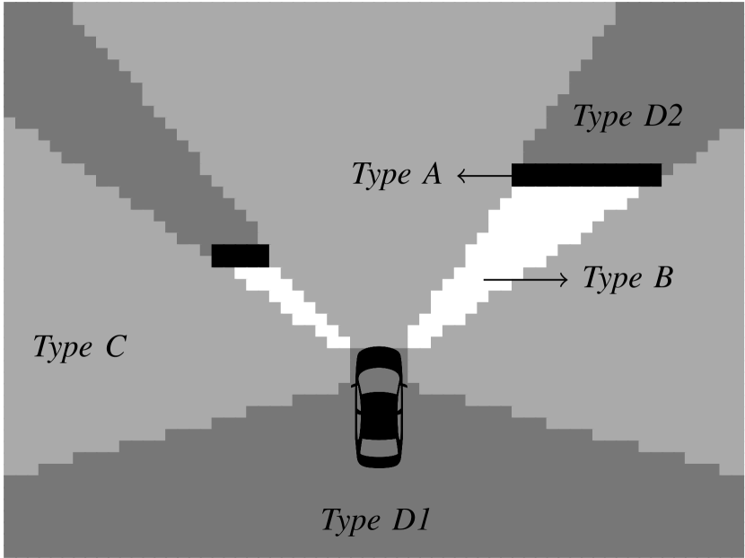
Figure 3: Schematic diagram showing four types of grid cells.

IV-B1 Conventional Choices for the Inverse Sensor Model

Since $\bm{z}_{k}$ provides no additional information on Type D grid cells, the occupancy in these cells is conditionally independent of $\bm{z}_{k}$, that is

$$p^{D}(O~{}|~{}\bm{z}_{k})=p(O)$$

where $p(O)$ is the prior probability of occupancy defined earlier in Sec. II-A.

Grid cells of Type B and Type C may be hypothesized to have low occupancy probability, since these grid cells were scanned by the sensor but no return was obtained. As a result, conventionally

$$p^{B}(O~{}|~{}\bm{z}_{k})\leq p(O)$$

and

$$p^{C}(O~{}|~{}\bm{z}_{k})\leq p(O)$$

Finally, grid cells of Type A may be hypothesized to have higher occupancy probability, since a return has been observed in the vicinity of these cells. Conventionally,

$$p^{A}(O~{}|~{}\bm{z}_{k})\geq p(O)$$

In the limit, if the OGM grid cell size is comparable to the sensor range and angle uncertainty, or if the number of scans is large enough such that the uncertainty is captured empirically, only the grid cells that contain the sensor measurement may be considered to be of Type A.

IV-B2 Automotive Radar Sensor Characteristics

Intense clutter properties and sparsity of the automotive radar data complicate the choice of the inverse sensor model.

Sparsity. First, sparsity of the radar scan implies that many occupied Type A grid cells in the radar environment might be incorrectly categorized as free Type C cells. This can be observed in Fig. 1. As evidenced by the batch of scans in Fig. 1, the radar environment is “dense” in that many grid cells contain radar reflectors. However, any individual radar scan, such as the one shown in Fig. 1, suggests a much more sparse radar environment. As a result, a grid cell which is occupied in truth will be incorrectly categorized as Type C in many scans, and correctly as Type A in a few scans.

The sparsity of radar returns also makes it challenging to distinguish Type C cells from cells of Type D2. Since many occluding obstacles are not detected in each scan, the occluded cells of Type D2 are conflated with free cells of Type C.

In context of the inverse sensor model, as the radar scan becomes more sparse

$$p^{C}(O~{}|~{}\bm{z}_{k})\rightarrow{p^{D}(O~{}|~{}\bm{z}_{k})}^{-}$$

where the superscript $-$ denotes a limit approaching from below. Intuitively, approaching $p^{D}(O~{}|~{}\bm{z}_{k})$ implies that the measurement $\bm{z}_{k}$ is very sparse in comparison to the true occupancy, and thus does not provide much information on lack of occupancy.

Clutter. Second, there is the matter of clutter. The grid cells in the vicinity of a clutter measurement may be incorrectly categorized as Type A, and the grid cells along the path between the radar and clutter measurement may be incorrectly categorized as Type B.

In context of the inverse sensor model, as the radar scan becomes more cluttered

$$p^{B}(O~{}|~{}\bm{z}_{k}) \rightarrow{p^{D}(O~{}|~{}\bm{z}_{k})}^{-}$$

$$p^{A}(O~{}|~{}\bm{z}_{k}) \rightarrow{p^{D}(O~{}|~{}\bm{z}_{k})}^{+}$$

where the superscript $+$ denotes a limit approaching from above.

IV-B3 A Pessimistic Inverse Sensor Model

The results presented in Sec. V are based on a pessimistic sensor model, such that $p^{B}(O~{}|~{}\bm{z}_{k})=p^{C}(O~{}|~{}\bm{z}_{k})=p^{D}(O~{}|~{}\bm{z}_{k})$. This model assumes that the radar measurements provide no information about free space in the radar environment.

In particular, the inverse sensor model assumes

$$p^{B}(O~{}|~{}\bm{z}_{k})=p^{C}(O~{}|~{}\bm{z}_{k})=p^{D}(O~{}|~{}\bm{z}_{k})=p(O)=0.1$$

and

$$p^{A}(O~{}|~{}\bm{z}_{k})=0.2$$

V Experimental Results

The radar-based urban positioning system was evaluated experimentally using the dataset described in [12], collected on Thursday, May 9, 2019 and Sunday, May 12, 2019 during approximately $1.5\text{\,}\mathrm{h}$ of driving each day in and around the urban center of Austin, TX. This section presents the evaluation results.

V-A Data Collection

Fig. 4 shows the route followed by the radar-instrumented vehicle. Of particular interest is the southern part of the route which combs through every street in the Austin, TX downtown area. Urban canyons are the most challenging for precise GNSS-based positioning [9] and would benefit the most from radar-based positioning. The route was driven once on a weekday and again on the weekend to evaluate robustness of the radar map to changes in traffic and parking patterns.

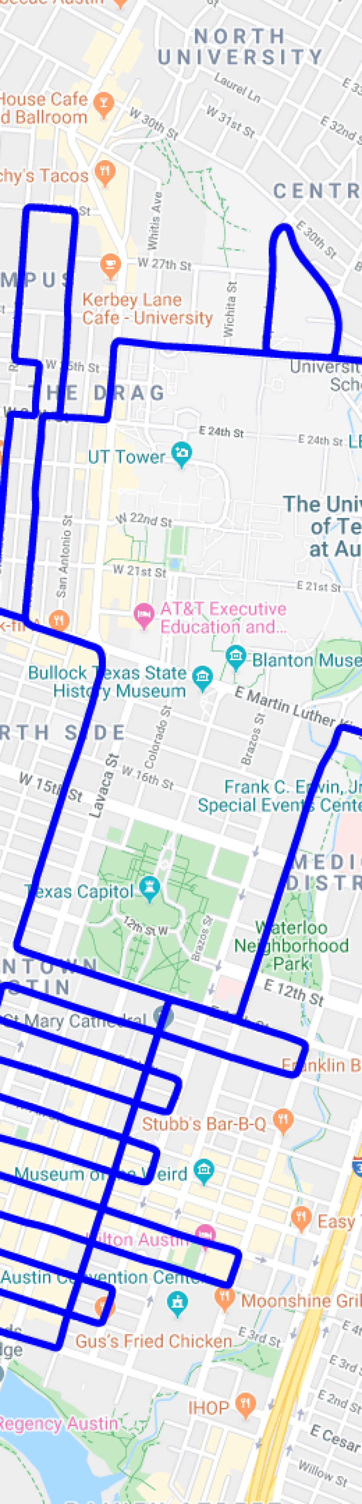
Figure 4: Test route through The University of Texas west campus and Austin downtown. These areas are the most challenging for precise GNSS-based positioning and thus would benefit the most from radar-based positioning. The route was driven once on a weekday and again on the weekend to evaluate robustness of the radar map to changes in traffic and parking patterns.

The Delphi electronically-scanning radar (ESR) and short-range radars (SRR2s) used in this study are mounted on an integrated perception platform called the Sensorium, shown schematically in Fig. 5. The coverage patterns of the radar units are shown in Fig. 6. The Sensorium’s onboard computer timestamps and logs the radar returns from the three radar units.

Figure 5: The University of Texas Sensorium is an integrated platform for automated and connected vehicle perception research. It includes three automotive radar units, one electronically-scanning radar (ESR) and two short-range radars (SRR2s); stereo visible light cameras; automotive- and industrial-grade inertial measurement units (IMUs); a dual-antenna, multi-frequency software-defined GNSS receiver; 4G cellular connectivity; and a powerful internal computer. An iXblue ATLANS-C CDGNSS-disciplined INS (not shown) is mounted at the rear of the platform to provide the ground truth trajectory.

Figure 6: Coverage patterns for the three Sensorium radar units. The ESR provides simultaneous sensing in a narrow ($\pm 10\text{\,}\mathrm{\SIUnitSymbolDegree}$) long-range ($175\text{\,}\mathrm{m}$) coverage area and a wider ($\pm 45\text{\,}\mathrm{\SIUnitSymbolDegree}$) medium-range ($60\text{\,}\mathrm{m}$) area. The SRR2 units each have a coverage area of $\pm 75\text{\,}\mathrm{\SIUnitSymbolDegree}$ and $80\text{\,}\mathrm{m}$. The line $l_{1}$ marks the left-most extent of the right SRR2’s field of view. Similarly, $l_{2}$ marks the right-most extent of the left SRR2’s field of view. Each SRR2 is installed facing outward from the centerline at an angle of $30\text{\,}\mathrm{\SIUnitSymbolDegree}$.

The reference position and orientation trajectory for the data are generated with the iXblue ATLANS-C: a high-performance RTK-GNSS coupled fiber-optic gyroscope (FOG) inertial navigation system (INS). The post-processed position solution obtained from the ATLANS-C is decimeter-accurate throughout the dataset.

(a)

(b)

(c)

Figure 7: This figure shows an interesting example of radar-based urban positioning with the proposed method. Panel (a) shows the occupancy grid estimated from the prior map point cloud. Panel (b) shows the same for a $5\text{\,}\mathrm{s}$ batch of scans collected in the same region. For ease of visualization, the batch occupancy grid has already been aligned with the map occupancy grid. Panel (c) shows the cross-correlation between the batch and map occupancy grids at $\Delta\phi=$ $0\text{\,}\mathrm{\SIUnitSymbolDegree}$. Given that no rotational or translational offset error has been applied to the batch, the correlation peak should appear at $(0,0)$. The offset of the peak in panel (c) from $(0,0)$ is the translational estimate error of the proposed method. Also note the increased positioning uncertainty in the along-track direction, and the two local correlation peaks (marked with red squares in panel (c)) due to the repeating periodic pattern of radar reflectors in the map and the batch (marked with red rectangles in panels (a) and (b)).

V-B Mapping

The first step to radar-based localization is generation of a radar map point cloud. Radar scans collected from the May 9, 2019 session are aggregated to create a map with the benefit of the ATLANS-C reference trajectory. The map point cloud is stored in a k-d tree for efficient querying during localization.

Two important notes are in order here. First, automotive radar clutter is especially intense when the vehicle is stationary. Accordingly, this paper disregards radar returns obtained when the vehicle is moving slower than $1\text{\,}\mathrm{m}\text{\,}{\mathrm{s}}^{-1}$ (approximately $2.23$ miles per hour) for both mapping and localization. This implies that radar-based localization is only available during periods when the vehicle is moving faster than $1\text{\,}\mathrm{m}\text{\,}{\mathrm{s}}^{-1}$. Second, it was observed that radar returns far from the vehicle are mostly clutter and have negligible resemblance to the surrounding structure. As a result, this paper only considers radar returns with range less than $50\text{\,}\mathrm{m}$. It must be noted that these two parameters have not been optimized to produce the smallest estimation errors; they have been fixed based on visual inspection.

V-C Localization Results with Perfect Odometry

This section evaluates the localization performance of the proposed method on the May 12, 2019 radar data for the case in which odometric drift over the radar batch-of-scans interval is negligible. With decreasing quality of the odometry sensor(s), this assumption holds only over ever shorter batch intervals. Therefore, the performance of the algorithm is evaluated for a range of batch lengths.

V-C1 Test procedure

A drift-free vehicle trajectory over a batch-of-scans interval is generated with the reference solution from the iXblue ATLANS-C. This trajectory is then artificially offset by a two-dimensional rigid transformation error. The translational error is distributed such that $\Delta\bm{t}\sim\mathcal{N}(\bm{0},\sigma_{t}^{2}I)$ with $\sigma_{t}=$ $2\text{\,}\mathrm{m}$, and the rotational error is distributed such that $\Delta\phi\sim\mathcal{N}(0,\sigma_{\phi}^{2})$ with $\sigma_{\phi}=$ $3\text{\,}\mathrm{\SIUnitSymbolDegree}$. The proposed localization technique takes the erroneously-offset position and heading trajectory as the initial guess of the vehicle state.

The prior radar map point cloud in the vicinity of the initial guess of the vehicle position is retrieved with a query to the k-d tree. Additionally, the batch of body-frame radar returns is transformed to a common reference frame based on the erroneous trajectory. The goal is to align the two point clouds and thereby estimate the artificially-induced translational and rotational offset.

As a first step, the map and batch occupancy grids are generated based on the aggregated point clouds, following the procedure described in Sec. II and IV. The extent of the occupancy grids is determined by the bounds of the area scanned by the radars during localization. Given the maximum range of radar returns considered here, the correlation region is typically restricted to $\pm 50\text{\,}\mathrm{m}$ around the provided position at the end of the batch. With a grid cell size of $10\text{\,}\mathrm{cm}$, the occupancy grid size in discrete coordinates is typically on the order of $n=1000$. The translation search space is limited to $\pm 3\sigma_{t}=\pm$ $6\text{\,}\mathrm{m}$, resulting in $n_{l}=120$. Similarly, the rotation search space is limited to $\pm 3\sigma_{\phi}=\pm$ $9\text{\,}\mathrm{\SIUnitSymbolDegree}$ with $1\text{\,}\mathrm{\SIUnitSymbolDegree}$ steps, resulting in $m=18$.

V-C2 Five-second Batches

This section evaluates and analyzes the proposed method for a fixed batch length of $5\text{\,}\mathrm{s}$. Fig. 7 shows an interesting example of radar-based urban positioning. For ease of visualization, no translation or rotation offset error has been applied to the batch point cloud. The occupancy grid estimated from the $5\text{\,}\mathrm{s}$ batch point cloud is shown in Fig. 7. Similarly, Fig. 7 shows the occupancy grid estimated from the map point cloud retrieved from the map database. Fig. 7 shows the cross correlation between the batch and map occupancy grids at $\Delta\phi=$ $0\text{\,}\mathrm{\SIUnitSymbolDegree}$. Given that no offset error has been applied to the batch, one should expect the correlation peak to appear at $(0,0)$ in Fig. 7. The offset of the peak from $(0,0)$ in this case is the translational estimate error.

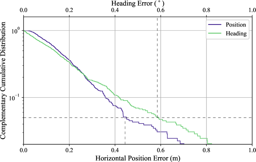
Figure 8: The complementary cumulative distribution (also known as a survival function) indicates how often (that is, in what fraction of $5\text{\,}\mathrm{s}$ epochs) the localization procedure in the text was found to exceed a given level of error. The logarithmic vertical scale makes the tails of the distribution, corresponding to outliers that may cause tracking errors, more visible. For $5\text{\,}\mathrm{s}$ batches, the 95-percentile horizontal positioning error is observed to be $44\text{\,}\mathrm{cm}$ and the 95-percentile heading error is observed to be $0.59\text{\,}\mathrm{\SIUnitSymbolDegree}$.

Two other interesting features of the cross-correlation in Fig. 7 are worth noting. First, the correlation peak decays slower in the along-track direction—in this case approximately aligned with the south-southwest direction. This is a general feature observed throughout the dataset, since most of the radar reflectors are aligned along the sides of the streets. Second, there emerge two local correlation peaks offset by $\approx$$4\text{\,}\mathrm{m}$ along the direction of travel. These local peaks are due to the repeating periodic structure of radar reflectors in both the map and the batch occupancy grids. In other words, shifting the batch occupancy grid forward or backward along the vehicle trajectory by $\approx$$4\text{\,}\mathrm{m}$ aligns the periodically-repeating reflectors in an off-by-one manner, leading to another plausible solution. Importantly, the uncertainty envelope of the initial position peak can span several meters, encompassing both the global optimum and one or more local optima. This explains why gradient-based methods, which seek the nearest optimum, are poorly suited for use with automotive radar.

The complementary cumulative distribution functions (CCDF), i.e., the fraction of epochs exceeding any given level of error, of the horizontal position and heading error magnitudes are plotted on a log scale in Fig. 8 for $5\text{\,}\mathrm{s}$ batches. In 95% of epochs, the horizontal position error magnitude was no greater than $44\text{\,}\mathrm{cm}$, and the heading error magnitude was no greater than $0.59\text{\,}\mathrm{\SIUnitSymbolDegree}$.

V-C3 Sensitivity to Batch Length

The assumption of negligible odometric drift over the batch-of-scans interval does not hold over $5\text{\,}\mathrm{s}$ for low-cost odometry sensors, but may hold for longer than $5\text{\,}\mathrm{s}$ for high-performance sensors. Thus, is important to evaluate the proposed localization technique’s sensitivity to batch length.

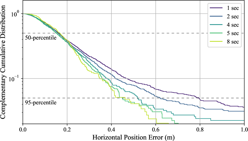
Figure 9: CCDFs for different batch lengths between $1\text{\,}\mathrm{s}$ and $8\text{\,}\mathrm{s}$. The $50$-percentile errors are similar for shorter and longer batch lengths, but the difference becomes more noticeable at higher percentiles.

Fig. 9 shows the CCDF for different batch lengths between $1\text{\,}\mathrm{s}$ and $8\text{\,}\mathrm{s}$. As expected, the errors are smaller for longer batch lengths. It is interesting to note that the $50$-percentile errors are similar for different batch lengths, but difference between the CCDFs becomes more pronounced at higher percentiles. This indicates that the shorter batch lengths are adequate in most cases, but the longer batches help contain the estimation error in a few cases. Such behavior must be taken into account in the integrity analysis of the system. For example, while all batch lengths exhibit similar $50$-percentile error behavior, batches shorter than $4\text{\,}\mathrm{s}$ cannot be used in applications with a $50\text{\,}\mathrm{cm}$ alert limit and integrity risk smaller than $0.05$ per batch. On the other hand, in applications where $50$-percentile error is the performance metric, it may be desirable to choose batches shorter than $4\text{\,}\mathrm{s}$ to relax the requirements on short term odometric performance.

V-D Sensitivity to Odometric Drift

Even over small batch durations, the odometric vehicle trajectory may exhibit non-negligible drift. While the proposed technique does not provide a means to estimate and eliminate such drift, it is important to study if such effects lead to catastrophic degradation in performance.

This section considers simple drift models for position and heading drift during batch generation. In particular, odometry-based orientation is typically computed as integrated angular rate (e.g., from a gyroscope), and odometry-based distance is typically derived as either integrated speed (e.g., with rotary encoders, radar-based odometry), or as double-integrated acceleration (e.g., with an accelerometer). To a coarse approximation, this section assumes that the largest source of error in odometry is due to integration of residual biases. This has the effect of a linear drift in orientation estimates and either linear (in case of integrated velocity measurements) or quadratic (in case of double-integrated acceleration) drift in position estimates.

Figure 10: CCDFs for $5\text{\,}\mathrm{s}$ batches with three different levels of trajectory drift during batch generation. The solid lines represent quadratic drift in position and linear drift in heading. The dashed lines represent linear drift in both position and heading. The three different colors represent standard deviation of the drift at the end of the $5\text{\,}\mathrm{s}$ interval: ($10\text{\,}\mathrm{cm}$, $0.25\text{\,}\mathrm{\SIUnitSymbolDegree}$), ($20\text{\,}\mathrm{cm}$, $0.5\text{\,}\mathrm{\SIUnitSymbolDegree}$), and ($40\text{\,}\mathrm{cm}$, $1\text{\,}\mathrm{\SIUnitSymbolDegree}$).

As before, a drift-free vehicle batch trajectory is obtained from the reference solution from the iXblue ATLANS-C. In addition to the rigid transformational offset error applied in the previous subsection, a time-dependent position and heading drift is introduced in to the batch trajectory. The trajectory is then used to transform the body-frame radar returns in to a common reference frame as before. Assuming that the odometric drift is small as compared to the rigid offset, the proposed approach is evaluated in its ability to estimate the rigid offset.

This section restricts the analysis to $5\text{\,}\mathrm{s}$ batches with three different levels of pose drift. The level of drift is characterized by the standard deviation of the position and heading error at the end of the $5\text{\,}\mathrm{s}$ interval. The three pairs of drift levels considered here are chosen such that they are relatively small as compared to $\sigma_{t}$ and $\sigma_{\phi}$: ($10\text{\,}\mathrm{cm}$, $0.25\text{\,}\mathrm{\SIUnitSymbolDegree}$), ($20\text{\,}\mathrm{cm}$, $0.5\text{\,}\mathrm{\SIUnitSymbolDegree}$), and ($40\text{\,}\mathrm{cm}$, $1\text{\,}\mathrm{\SIUnitSymbolDegree}$). Both the linear and quadratic error growth models for position drift are explored.

Fig. 10 shows the CCDF plots for different levels of odometric drift and different position drift models. As expected, the performance degrades with larger drift during batch generation. Nevertheless, the effect of impairment is not catastrophic—with quadratic position and linear heading drift standard deviation of $40\text{\,}\mathrm{cm}$ and $1\text{\,}\mathrm{\SIUnitSymbolDegree}$ at $5\text{\,}\mathrm{s}$, respectively, the $95$-percentile error in estimation of the rigid offset is $67\text{\,}\mathrm{cm}$ and $1.17\mathrm{°}$.

VI Conclusion

A novel technique for robust 50-cm-accurate urban ground positioning based on commercially-available low-cost automotive radars has been proposed. This is a significant development in the field of AGV localization, which has traditionally been based on sensors such as lidar and cameras that perform poorly in bad weather conditions. The proposed technique is computationally efficient yet obtains a globally-optimal translation and heading solution, avoiding local minima caused by repeating patterns in the urban radar environment. Performance evaluation on an extensive and realistic urban data set shows that, when coupled with stable short-term odometry, the technique maintains $95$-percentile errors below $50\text{\,}\mathrm{cm}$ in horizontal position and $1\mathrm{°}$ in heading.

References

- [1] D. Fajardo, T.-C. Au, S. Waller, P. Stone, and D. Yang, “Automated intersection control: Performance of future innovation versus current traffic signal control,” Transportation Research Record: Journal of the Transportation Research Board, no. 2259, pp. 223–232, 2011.
- [2] J. Choi, V. Va, N. Gonzalez-Prelcic, R. Daniels, C. R. Bhat, and R. W. Heath, “Millimeter-wave vehicular communication to support massive automotive sensing,” IEEE Communications Magazine, vol. 54, no. 12, pp. 160–167, December 2016.
- [3] D. LaChapelle, T. E. Humphreys, L. Narula, P. A. Iannucci, and E. Moradi-Pari, “Automotive collision risk estimation under cooperative sensing,” in Proceedings of the IEEE International Conference on Acoustics, Speech, and Signal Processing, Barcelona, Spain, 2020.
- [4] K. S. Yen, C. Shankwitz, B. Newstrom, T. A. Lasky, and B. Ravani, “Evaluation of the University of Minnesota GPS Snowplow Driver Assistance Program,” Tech. Rep., 2015.
- [5] M. Petovello, M. Cannon, and G. Lachapelle, “Benefits of using a tactical-grade IMU for high-accuracy positioning,” Navigation, Journal of the Institute of Navigation, vol. 51, no. 1, pp. 1–12, 2004.
- [6] B. M. Scherzinger, “Precise robust positioning with inertially aided RTK,” Navigation, vol. 53, no. 2, pp. 73–83, 2006.
- [7] H. T. Zhang, “Performance comparison on kinematic GPS integrated with different tactical-grade IMUs,” Master’s thesis, The University of Calgary, Jan. 2006.
- [8] S. Kennedy, J. Hamilton, and H. Martell, “Architecture and system performance of SPAN—NovAtel’s GPS/INS solution,” in Position, Location, And Navigation Symposium, 2006 IEEE/ION. IEEE, 2006, p. 266.
- [9] T. E. Humphreys, L. Narula, and M. J. Murrian, “Deep urban unaided precise GNSS vehicle positioning,” IEEE Intelligent Transportation Systems Magazine, 2020, to be published.
- [10] T. E. Humphreys, Springer Handbook of Global Navigation Satellite Systems. Springer, 2017, ch. Interference, pp. 469–504.
- [11] L. Narula, J. M. Wooten, M. J. Murrian, D. M. LaChapelle, and T. E. Humphreys, “Accurate collaborative globally-referenced digital mapping with standard GNSS,” Sensors, vol. 18, no. 8, 2018. [Online]. Available: http://www.mdpi.com/1424-8220/18/8/2452
- [12] L. Narula, D. M. LaChapelle, M. J. Murrian, J. M. Wooten, T. E. Humphreys, J.-B. Lacambre, E. de Toldi, and G. Morvant, “TEX-CUP: The University of Texas Challenge for Urban Positioning,” in Proceedings of the IEEE/ION PLANS Meeting, Portland, OR, 2020, to be published.
- [13] R. P. Mahler, “Multitarget Bayes filtering via first-order multitarget moments,” IEEE Transactions on Aerospace and Electronic systems, vol. 39, no. 4, pp. 1152–1178, 2003.
- [14] A. Myronenko and X. Song, “Point set registration: Coherent point drift,” IEEE Transactions on Pattern Analysis and Machine Intelligence, vol. 32, no. 12, pp. 2262–2275, 2010.
- [15] B. Jian and B. C. Vemuri, “Robust point set registration using Gaussian mixture models,” IEEE Transactions on Pattern Analysis and Machine Intelligence, vol. 33, no. 8, pp. 1633–1645, 2010.
- [16] O. Erdinc, P. Willett, and Y. Bar-Shalom, “The bin-occupancy filter and its connection to the PHD filters,” IEEE Transactions on Signal Processing, vol. 57, no. 11, pp. 4232–4246, 2009.
- [17] S. Thrun, W. Burgard, and D. Fox, Probabilistic robotics. MIT press, 2005.
- [18] D. Chetverikov, D. Svirko, D. Stepanov, and P. Krsek, “The trimmed iterative closest point algorithm,” in Object recognition supported by user interaction for service robots, vol. 3. IEEE, 2002, pp. 545–548.
- [19] E. Ward and J. Folkesson, “Vehicle localization with low cost radar sensors,” in 2016 IEEE Intelligent Vehicles Symposium (IV). IEEE, 2016, pp. 864–870.
- [20] Y. Tsin and T. Kanade, “A correlation-based approach to robust point set registration,” in European conference on computer vision. Springer, 2004, pp. 558–569.
- [21] W. Gao and R. Tedrake, “FilterReg: Robust and efficient probabilistic point-set registration using gaussian filter and twist parameterization,” in Proceedings of the IEEE Conference on Computer Vision and Pattern Recognition, 2019, pp. 11 095–11 104.
- [22] S. H. Cen and P. Newman, “Radar-only ego-motion estimation in difficult settings via graph matching,” arXiv preprint arXiv:1904.11476, 2019.
- [23] M. Holder, S. Hellwig, and H. Winner, “Real-time pose graph SLAM based on radar,” in 2019 IEEE Intelligent Vehicles Symposium (IV). IEEE, 2019, pp. 1145–1151.
- [24] F. Schuster, C. G. Keller, M. Rapp, M. Haueis, and C. Curio, “Landmark based radar SLAM using graph optimization,” in Intelligent Transportation Systems (ITSC), 2016 IEEE 19th International Conference on. IEEE, 2016, pp. 2559–2564.
- [25] M. Schoen, M. Horn, M. Hahn, and J. Dickmann, “Real-time radar SLAM.”
- [26] J. Callmer, D. Törnqvist, F. Gustafsson, H. Svensson, and P. Carlbom, “Radar SLAM using visual features,” EURASIP Journal on Advances in Signal Processing, vol. 2011, no. 1, p. 71, 2011.
- [27] K. Yoneda, N. Hashimoto, R. Yanase, M. Aldibaja, and N. Suganuma, “Vehicle localization using 76GHz omnidirectional millimeter-wave radar for winter automated driving,” in 2018 IEEE Intelligent Vehicles Symposium (IV). IEEE, 2018, pp. 971–977.
- [28] J. Mullane, B.-N. Vo, M. D. Adams, and B.-T. Vo, “A random-finite-set approach to Bayesian SLAM,” IEEE Transactions on Robotics, vol. 27, no. 2, pp. 268–282, 2011.
- [29] H. Deusch, S. Reuter, and K. Dietmayer, “The labeled multi-Bernoulli SLAM filter,” IEEE Signal Processing Letters, vol. 22, no. 10, pp. 1561–1565, 2015.
- [30] M. Stübler, S. Reuter, and K. Dietmayer, “A continuously learning feature-based map using a Bernoulli filtering approach,” in 2017 Sensor Data Fusion: Trends, Solutions, Applications (SDF). IEEE, 2017, pp. 1–6.
- [31] M. Fatemi, K. Granström, L. Svensson, F. J. Ruiz, and L. Hammarstrand, “Poisson multi-bernoulli mapping using Gibbs sampling,” IEEE Transactions on Signal Processing, vol. 65, no. 11, pp. 2814–2827, 2017.
- [32] B. S. Reddy and B. N. Chatterji, “An FFT-based technique for translation, rotation, and scale-invariant image registration,” IEEE transactions on image processing, vol. 5, no. 8, pp. 1266–1271, 1996.