DagoBERT: Generating Derivational Morphology
with a Pretrained Language Model

Abstract

Can pretrained language models (PLMs) generate derivationally complex words? We present the first study investigating this question, taking BERT as the example PLM. We examine BERT’s derivational capabilities in different settings, ranging from using the unmodified pretrained model to full finetuning. Our best model, DagoBERT (Derivationally and generatively optimized BERT), clearly outperforms the previous state of the art in derivation generation (DG). Furthermore, our experiments show that the input segmentation crucially impacts BERT’s derivational knowledge, suggesting that the performance of PLMs could be further improved if a morphologically informed vocabulary of units were used.

1 Introduction

What kind of linguistic knowledge is encoded by pretrained language models (PLMs) such as ELMo (Peters et al., 2018), GPT-2 (Radford et al., 2019), and BERT (Devlin et al., 2019)? This question has attracted a lot of attention in NLP recently, with a focus on syntax (e.g., Goldberg, 2019) and semantics (e.g., Ethayarajh, 2019). It is much less clear what PLMs learn about other aspects of language. Here, we present the first study on the knowledge of PLMs about derivational morphology, taking BERT as the example PLM. Given an English cloze sentence such as this jacket is           . and a base such as wear, we ask: can BERT generate correct derivatives such as unwearable?

The motivation for this study is twofold. On the one hand, we add to the growing body of work on the linguistic capabilities of PLMs. Most PLMs segment words into subword units (Bostrom and Durrett, 2020), e.g., unwearable is segmented into un, ##wear, ##able by BERT’s WordPiece tokenizer (Wu et al., 2016). The fact that many of these subword units are derivational affixes suggests that PLMs might acquire knowledge about derivational morphology (Table 1), but this has not been tested. On the other hand, we are interested in derivation generation (DG) per se, a task that has been only addressed using LSTMs (Cotterell et al., 2017; Vylomova et al., 2017; Deutsch et al., 2018), not models based on Transformers like BERT.

[width=]dagobert-tikz

Figure 1: Basic experimental setup. We input sentences such as this jacket is unwearable . to BERT, mask out derivational affixes, and recover them using a derivational classification layer (DCL).

Type	Examples
Prefixes	anti, auto, contra, extra, hyper, mega, mini, multi, non, proto, pseudo
Suffixes	##able, ##an, ##ate, ##ee, ##ess, ##ful, ##ify, ##ize, ##ment, ##ness, ##ster

Table 1: Examples of derivational affixes in the BERT WordPiece vocabulary. Word-internal WordPiece tokens are marked with ## throughout the paper.

Contributions. We develop the first framework for generating derivationally complex English words with a PLM, specifically BERT, and analyze BERT’s performance in different settings. Our best model, DagoBERT (Derivationally and generatively optimized BERT), clearly outperforms an LSTM-based model, the previous state of the art. We find that DagoBERT’s errors are mainly due to syntactic and semantic overlap between affixes. Furthermore, we show that the input segmentation impacts how much derivational knowledge is available to BERT, both during training and inference. This suggests that the performance of PLMs could be further improved if a morphologically informed vocabulary of units were used. We also publish the largest dataset of derivatives in context to date.

2 Derivational Morphology

Linguistics divides morphology into inflection and derivation. Given a lexeme such as wear, while inflection produces word forms such as wears, derivation produces new lexemes such as unwearable. There are several differences between inflection and derivation (Haspelmath and Sims, 2010), two of which are particularly important for the task of DG.

First, derivation covers a much larger spectrum of meanings than inflection (Acquaviva, 2016), and it is not possible to predict in general with which of them a particular lexeme is compatible. This is different from inflectional paradigms, where it is automatically clear whether a certain form will exist (Bauer, 2019). Second, the relationship between form and meaning is more varied in derivation than inflection. On the one hand, derivational affixes tend to be highly polysemous, i.e., individual affixes can represent a number of related meanings (Lieber, 2019). On the other hand, several affixes can represent the same meaning, e.g., ity and ness. While such competing affixes are often not completely synonymous as in the case of hyperactivity and hyperactiveness, there are examples like purity and pureness or exclusivity and exclusiveness where a semantic distinction is more difficult to gauge (Bauer et al., 2013; Plag and Balling, 2020). These differences make learning functions from meaning to form harder for derivation than inflection.

Derivational affixes differ in how productive they are, i.e., how readily they can be used to create new lexemes (Plag, 1999). While the suffix ness, e.g., can attach to practically all English adjectives, the suffix th is much more limited in its scope of applicability. In this paper, we focus on productive affixes such as ness and exclude unproductive affixes such as th. Morphological productivity has been the subject of much work in psycholinguistics since it reveals implicit cognitive generalizations (see Dal and Namer (2016) for a review), making it an interesting phenomenon to explore in PLMs. Furthermore, in the context of NLP applications such as sentiment analysis, productively formed derivatives are challenging because they tend to have very low frequencies and often only occur once (i.e., they are hapaxes) or a few times in large corpora (Mahler et al., 2017). Our focus on productive derivational morphology has crucial consequences for dataset design (Section 3) and model evaluation (Section 4) in the context of DG.

3 Dataset of Derivatives

		P			S			PS
Bin	$\mu_{f}$	$n_{d}$	$n_{s}$	Examples	$n_{d}$	$n_{s}$	Examples	$n_{d}$	$n_{s}$	Examples
B1	.041	60,236	60,236	antijonny	39,543	39,543	takeoverness	20,804	20,804	unaggregateable
B2	.094	39,181	90,857	antiastronaut	22,633	52,060	alaskaness	8,661	19,903	unnicknameable
B3	.203	26,967	135,509	antiyale	14,463	71,814	blockbusterness	4,735	23,560	unbroadcastable
B4	.423	18,697	196,295	antihomework	9,753	100,729	abnormalness	2,890	29,989	unbrewable
B5	.868	13,401	287,788	antiboxing	6,830	145,005	legalness	1,848	39,501	ungooglable
B6	1.750	9,471	410,410	antiborder	4,934	211,233	tragicness	1,172	50,393	uncopyrightable
B7	3.515	6,611	573,442	antimafia	3,580	310,109	lightweightness	802	69,004	unwashable

Table 2: Data summary statistics. The table shows statistics of the data used in the study by frequency bin and affix type. We also provide example derivatives with anti (P), ness (S), and un##able (PS) for the different bins. $\mu_{f}$: mean frequency per billion words; $n_{d}$: number of distinct derivatives; $n_{s}$: number of context sentences.

We base our study on a new dataset of derivatives in context similar in form to the one released by Vylomova et al. (2017), i.e., it is based on sentences with a derivative (e.g., this jacket is unwearable .) that are altered by masking the derivative (this jacket is           .). Each item in the dataset consists of (i) the altered sentence, (ii) the derivative (unwearable) and (iii) the base (wear). The task is to generate the correct derivative given the altered sentence and the base. We use sentential contexts rather than tags to represent derivational meanings because they better reflect the semantic variability inherent in derivational morphology (Section 2). While Vylomova et al. (2017) use Wikipedia, we extract the dataset from Reddit. Since productively formed derivatives are not part of the language norm initially (Bauer, 2001), social media is a particularly fertile ground for our study.

For determining derivatives, we use the algorithm introduced by Hofmann et al. (2020a), which takes as input a set of prefixes, suffixes, and bases and checks for each word in the data whether it can be derived from a base using a combination of prefixes and suffixes. The algorithm is sensitive to morpho-orthographic rules of English Plag (2003), e.g., when ity is removed from applicability, the result is applicable, not applicabil. Here, we use BERT’s prefixes, suffixes, and bases as input to the algorithm. Drawing upon a comprehensive list of 52 productive prefixes and 49 productive suffixes in English (Crystal, 1997), we find that 48 and 44 of them are contained in BERT’s vocabulary. We assign all fully alphabetic words with more than 3 characters in BERT’s vocabulary except for stopwords and previously identified affixes to the set of bases, yielding a total of 20,259 bases. We then extract every sentence including a word that is derivable from one of the bases using at least one of the prefixes or suffixes from all publicly available Reddit posts.

The sentences are filtered to contain between 10 and 100 words, i.e., they provide more contextual information than the example sentence above. See Appendix A.1 for details about data preprocessing. The resulting dataset comprises 413,271 distinct derivatives in 123,809,485 context sentences, making it more than two orders of magnitude larger than the one released by Vylomova et al. (2017). To get a sense of segmentation errors in the dataset, we randomly pick 100 derivatives for each affix and manually count missegmentations. We find that the average precision of segmentations in the sample is .960$\pm$.074, with higher values for prefixes (.990$\pm$.027) than suffixes (.930$\pm$.093).

For this study, we extract all derivatives with a frequency $f\in[1,128)$ from the dataset. We divide the derivatives into 7 frequency bins with $f=1$ (B1), $f\in[2,4)$ (B2), $f\in[4,8)$ (B3), $f\in[8,16)$ (B4), $f\in[16,32)$ (B5), $f\in[32,64)$ (B6), and $f\in[64,128)$ (B7). Notice that we focus on low-frequency derivatives since we are interested in productive derivational morphology (Section 2). In addition, BERT is likely to have seen high-frequency derivatives multiple times during pretraining and might be able to predict the affix because it has memorized the connection between the base and the affix, not because it has knowledge of derivational morphology. BERT’s pretraining corpus has 3.3 billion words, i.e., words in the lower frequency bins are very unlikely to have been seen by BERT before. This observation also holds for average speakers of English, who have been shown to encounter at most a few billion word tokens in their lifetime (Brysbaert et al., 2016).

Regarding the number of affixes, we confine ourselves to three cases: derivatives with one prefix (P), derivatives with one suffix (S), and derivatives with one prefix and one suffix (PS). We treat these cases separately because they are known to have different linguistic properties. In particular, since suffixes in English can change the POS of a lexeme, the syntactic context is more affected by suffixation than by prefixation. Table 2 provides summary statistics for the seven frequency bins as well as example derivatives for P, S, and PS. For each bin, we randomly split the data into 60% training, 20% development, and 20% test. Following Vylomova et al. (2017), we distinguish the lexicon settings SPLIT (no overlap between bases in train, dev, and test) and SHARED (no constraint on overlap).

4 Experiments

4.1 Setup

To examine whether BERT can generate derivationally complex words, we use a cloze test: given a sentence with a masked word such as this jacket is           . and a base such as wear, the task is to generate the correct derivative such as unwearable. The cloze setup has been previously used in psycholinguistics to probe derivational morphology (Pierrehumbert, 2006; Apel and Lawrence, 2011) and was introduced to NLP in this context by Vylomova et al. (2017).

In this work, we frame DG as an affix classification task, i.e., we predict which affix is most likely to occur with a given base in a given context sentence. More formally, given a base $b$ and a context sentence $\mathbf{x}$ split into left and right contexts $\mathbf{x}^{(l)}=(x_{1},\dots,x_{d-1})$ and $\mathbf{x}^{(r)}=(x_{d+1},\dots,x_{n})$, with $x_{d}$ being the masked derivative, we want to find the affix $\hat{a}$ such that

$$\hat{a}=\operatorname*{arg\,max}_{a}P\left(\psi(b,a)|\mathbf{x}^{(l)},\mathbf{x}^{(r)}\right),$$ (1)

where $\psi$ is a function mapping bases and affixes onto derivatives, e.g., $\psi(\text{{wear}},\text{{un\#\#able}})=\text{{unwearable}}$. Notice we do not model the function $\psi$ itself, i.e., we only predict derivational categories, not the morpho-orthographic changes that accompany their realization in writing. One reason for this is that as opposed to previous work, our study focuses on low-frequency derivatives, for many of which $\psi$ is not right-unique, e.g., ungoogleable and ungooglable or celebrityness and celebritiness occur as competing forms in the data.

As a result of the semantically diverse nature of derivation (Section 2), deciding whether a particular prediction $\hat{a}$ is correct or not is less straightforward than it may seem. Taking again the example sentence this jacket is           . with the masked derivative unwearable, compare the following five predictions:

• $\psi(b,\hat{a})=\text{{wearity}}$: ill-formed;

• $\psi(b,\hat{a})=\text{{wearer}}$: well-formed, syntactically incorrect (wrong POS);

• $\psi(b,\hat{a})=\text{{intrawearable}}$: well-formed, syntactically correct, semantically dubious;

• $\psi(b,\hat{a})=\text{{superwearable}}$: well-formed, syntactically correct, semantically possible, but did not occur in the example sentence;

• $\psi(b,\hat{a})=\text{{unwearable}}$: well-formed, syntactically correct, semantically possible, and did occur in the example sentence.

These predictions reflect increasing degrees of derivational knowledge. A priori, where to draw the line between correct and incorrect predictions on this continuum is not clear, especially with respect to the last two cases. Here, we apply the most conservative criterion: a prediction $\hat{a}$ is only judged correct if $\psi(b,\hat{a})=x_{d}$, i.e., if $\hat{a}$ is the affix in the masked derivative. Thus, we ignore affixes that might potentially produce equally possible derivatives such as superwearable.

We use mean reciprocal rank (MRR), macro-averaged over affixes, as the evaluation measure (Radev et al., 2002). We calculate the MRR value of an individual affix $a$ as

$$\operatorname{MRR}_{a}=\frac{1}{|D_{a}|}\sum_{i\in D_{a}}\operatorname{R}_{i}^{-1},$$ (2)

where $D_{a}$ is the set of derivatives containing $a$, and $\operatorname{R}_{i}$ is the predicted rank of $a$ for derivative $i$. We set $\operatorname{R}_{i}^{-1}=0$ if $\operatorname{R}_{i}>10$. Denoting with $\mathcal{A}$ the set of all affixes, the final MRR value is given by

$$\operatorname{MRR}=\frac{1}{|\mathcal{A}|}\sum_{a\in\mathcal{A}}\operatorname{MRR}_{a}.$$ (3)

4.2 Segmentation Methods

Method	B1	B2	B3	B4	B5	B6	B7	$\mu\pm\sigma$
HYP	.197	.228	.252	.278	.300	.315	.337	.272$\pm$.046
INIT	.184	.201	.211	.227	.241	.253	.264	.226$\pm$.027
TOK	.141	.157	.170	.193	.218	.245	.270	.199$\pm$.044
PROJ	.159	.166	.159	.175	.175	.184	.179	.171$\pm$.009

Table 3: Performance (MRR) of pretrained BERT for prefix prediction with different segmentations. Best score per column in gray, second-best in light-gray.

Since BERT distinguishes word-initial (wear) from word-internal (##wear) tokens, predicting prefixes requires the word-internal form of the base. However, only 795 bases in BERT’s vocabulary have a word-internal form. Take as an example the word unallowed: both un and allowed are in the BERT vocabulary, but we need the token ##allowed, which does not exist (BERT tokenizes the word into una, ##llo, ##wed). To overcome this problem, we test the following four segmentation methods:

	SHARED								SPLIT
Model	B1	B2	B3	B4	B5	B6	B7	$\mu\pm\sigma$	B1	B2	B3	B4	B5	B6	B7	$\mu\pm\sigma$
DagoBERT	.373	.459	.657	.824	.895	.934	.957	.728$\pm$.219	.375	.386	.390	.411	.412	.396	.417	.398$\pm$.014
BERT+	.296	.380	.497	.623	.762	.838	.902	.614$\pm$.215	.303	.313	.325	.340	.341	.353	.354	.333$\pm$.018
BERT	.197	.228	.252	.278	.300	.315	.337	.272$\pm$.046	.199	.227	.242	.279	.305	.307	.351	.273$\pm$.049
LSTM	.152	.331	.576	.717	.818	.862	.907	.623$\pm$.266	.139	.153	.142	.127	.121	.123	.115	.131$\pm$.013
RB	.064	.067	.064	.067	.065	.063	.066	.065$\pm$.001	.068	.064	.062	.064	.062	.064	.064	.064$\pm$.002

Table 4: Performance (MRR) of prefix (P) models. Best score per column in gray, second-best in light-gray.

	SHARED								SPLIT
Model	B1	B2	B3	B4	B5	B6	B7	$\mu\pm\sigma$	B1	B2	B3	B4	B5	B6	B7	$\mu\pm\sigma$
DagoBERT	.427	.525	.725	.868	.933	.964	.975	.774$\pm$.205	.424	.435	.437	.425	.421	.393	.414	.421$\pm$.014
BERT+	.384	.445	.550	.684	.807	.878	.921	.667$\pm$.197	.378	.387	.389	.380	.364	.364	.342	.372$\pm$.015
BERT	.229	.246	.262	.301	.324	.349	.381	.299$\pm$.052	.221	.246	.268	.299	.316	.325	.347	.289$\pm$.042
LSTM	.217	.416	.669	.812	.881	.923	.945	.695$\pm$.259	.188	.186	.173	.154	.147	.145	.140	.162$\pm$.019
RB	.071	.073	.069	.068	.068	.068	.068	.069$\pm$.002	.070	.069	.069	.071	.070	.069	.068	.069$\pm$.001

Table 5: Performance (MRR) of suffix (S) models. Best score per column in gray, second-best in light-gray.

	SHARED								SPLIT
Model	B1	B2	B3	B4	B5	B6	B7	$\mu\pm\sigma$	B1	B2	B3	B4	B5	B6	B7	$\mu\pm\sigma$
DagoBERT	.143	.355	.621	.830	.914	.940	.971	.682$\pm$.299	.137	.181	.199	.234	.217	.270	.334	.225$\pm$.059
BERT+	.103	.205	.394	.611	.754	.851	.918	.548$\pm$.296	.091	.128	.145	.182	.173	.210	.218	.164$\pm$.042
BERT	.082	.112	.114	.127	.145	.155	.190	.132$\pm$.032	.076	.114	.130	.177	.172	.226	.297	.170$\pm$.069
LSTM	.020	.338	.647	.781	.839	.882	.936	.635$\pm$.312	.015	.019	.026	.034	.041	.072	.081	.041$\pm$.024
RB	.002	.003	.003	.005	.006	.008	.012	.006$\pm$.003	.002	.004	.003	.006	.006	.007	.009	.005$\pm$.002

Table 6: Performance (MRR) of prefix-suffix (PS) models. Best score per column in gray, second-best in light-gray.

HYP. We insert a hyphen between the prefix and the base in its word-initial form, yielding the tokens un, -, allowed in our example. Since both prefix and base are guaranteed to be in the BERT vocabulary (Section 3), and since there are no tokens starting with a hyphen in the BERT vocabulary, BERT always tokenizes words of the form prefix-hyphen-base into prefix, hyphen, and base, making this a natural segmentation for BERT.

INIT. We simply use the word-initial instead of the word-internal form, segmenting the derivative into the prefix followed by the base, i.e., un, allowed in our example. Notice that this looks like two individual words to BERT since allowed is a word-initial unit.

TOK. To overcome the problem of INIT, we segment the base into word-internal tokens, i.e., our example is segmented into un, ##all, ##owed. This means that we use the word-internal counterpart of the base in cases where it exists.

PROJ. We train a projection matrix that maps embeddings of word-initial forms of bases to word-internal embeddings. More specifically, we fit a matrix $\hat{\mathbf{T}}\in\mathbb{R}^{m\times m}$ ($m$ being the embedding size) via least squares,

$$\hat{\mathbf{T}}=\operatorname*{arg\,min}_{\mathbf{T}}||\mathbf{E}\mathbf{T}-\mathbf{E}_{\#\#}||^{2}_{2},$$ (4)

where $\mathbf{E},\mathbf{E}_{\#\#}\in\mathbb{R}^{n\times m}$ are the word-initial and word-internal token input embeddings of bases with both forms. We then map bases with no word-internal form and a word-initial input token embedding $\mathbf{e}$ such as allow onto the projected word-internal embedding $\mathbf{e}^{\top}\hat{\mathbf{T}}$.

We evaluate the four segmentation methods on the SHARED test data for P with pretrained BERT_BASE, using its pretrained language modeling head for prediction and filtering for prefixes. The HYP segmentation method performs best (Table 3) and is adopted for BERT models on P and PS.

Model	SHARED	SPLIT
DagoBERT	.943	.615
LSTM	.824	.511
LSTM (V)	.830	.520

Table 7: Performance on Vylomova et al. (2017) dataset. We report accuracies for comparability. LSTM (V): LSTM in Vylomova et al. (2017). Best score per column in gray, second-best in light-gray.

4.3 Models

Type	Clusters
Prefixes	$\{$bi, demi, fore, mini, proto, pseudo, semi, sub, tri$\}$, $\{$arch, extra, hyper, mega, poly, super, ultra$\}$, $\{$anti, contra, counter, neo, pro$\}$, $\{$mal, mis, over, under$\}$, $\{$inter, intra$\}$, $\{$auto, de, di, in, re, sur, un$\}$, $\{$ex, vice$\}$, $\{$non, post, pre$\}$
Suffixes	$\{$##al, ##an, ##ial, ##ian, ##ic, ##ite$\}$, $\{$##en, ##ful, ##ive, ##ly, ##y$\}$, $\{$##able, ##ish, ##less$\}$, $\{$##age, ##ance, ##ation, ##dom, ##ery, ##ess, ##hood, ##ism, ##ity, ##ment, ##ness$\}$, $\{$##ant, ##ee, ##eer, ##er, ##ette, ##ist, ##ous, ##ster$\}$, $\{$##ate, ##ify, ##ize$\}$

Table 8: Prefix and suffix clusterings produced by Girvan-Newman after 4 graph splits on the DagoBERT confusion matrix. For reasons of space, we do not list clusters consisting of only one affix.

All BERT models use BERT_BASE and add a derivational classification layer (DCL) with softmax activation for prediction (Figure 1). We examine three BERT models and two baselines. See Appendix A.2 for details about implementation, hyperparameter tuning, and runtime.

DagoBERT. We finetune both BERT and DCL on DG, a model that we call DagoBERT (short for Derivationally and generatively optimized BERT). Notice that since BERT cannot capture statistical dependencies between masked tokens (Yang et al., 2019), all BERT-based models predict prefixes and suffixes independently in the case of PS.

BERT+. We keep the model weights of pretrained BERT fixed and only train DCL on DG. This is similar in nature to a probing task.

BERT. We use pretrained BERT and leverage its pretrained language modeling head as DCL, filtering for affixes, e.g., we compute the softmax only over prefixes in the case of P.

LSTM. We adapt the approach described in Vylomova et al. (2017), which combines the left and right contexts $\mathbf{x}^{(l)}$ and $\mathbf{x}^{(r)}$ of the masked derivative by means of two BiLSTMs with a character-level representation of the base. To allow for a direct comparison with BERT, we do not use the character-based decoder proposed by Vylomova et al. (2017) but instead add a dense layer for the prediction. For PS, we treat prefix-suffix bundles as units (e.g., un##able).

In order to provide a strict comparison to Vylomova et al. (2017), we also evaluate our LSTM and best BERT-based model on the suffix dataset released by Vylomova et al. (2017) against the reported performance of their encoder-decoder model. Notice Vylomova et al. (2017) show that providing the LSTM with the POS of the derivative increases performance. Here, we focus on the more general case where the POS is not known and hence do not consider this setting.

Random Baseline (RB). The prediction is a random ranking of all affixes.

5 Results

5.1 Overall Performance

Results are shown in Tables 4, 5, and 6. For P and S, DagoBERT clearly performs best. Pretrained BERT is better than LSTM on SPLIT but worse on SHARED. BERT+ performs better than pretrained BERT, even on SPLIT (except for S on B7). S has higher scores than P for all models and frequency bins, which might be due to the fact that suffixes carry POS information and hence are easier to predict given the syntactic context. Regarding frequency effects, the models benefit from higher frequencies on SHARED since they can connect bases with certain groups of affixes. For PS, DagoBERT also performs best in general but is beaten by LSTM on one bin. The smaller performance gap as compared to P and S can be explained by the fact that DagoBERT as opposed to LSTM cannot learn statistical dependencies between two masked tokens (Section 4).

The results on the dataset released by Vylomova et al. (2017) confirm the superior performance of DagoBERT (Table 7). DagoBERT beats the LSTM by a large margin, both on SHARED and SPLIT. We also notice that our LSTM (which predicts derivational categories) has a very similar performance to the LSTM encoder-decoder proposed by Vylomova et al. (2017).

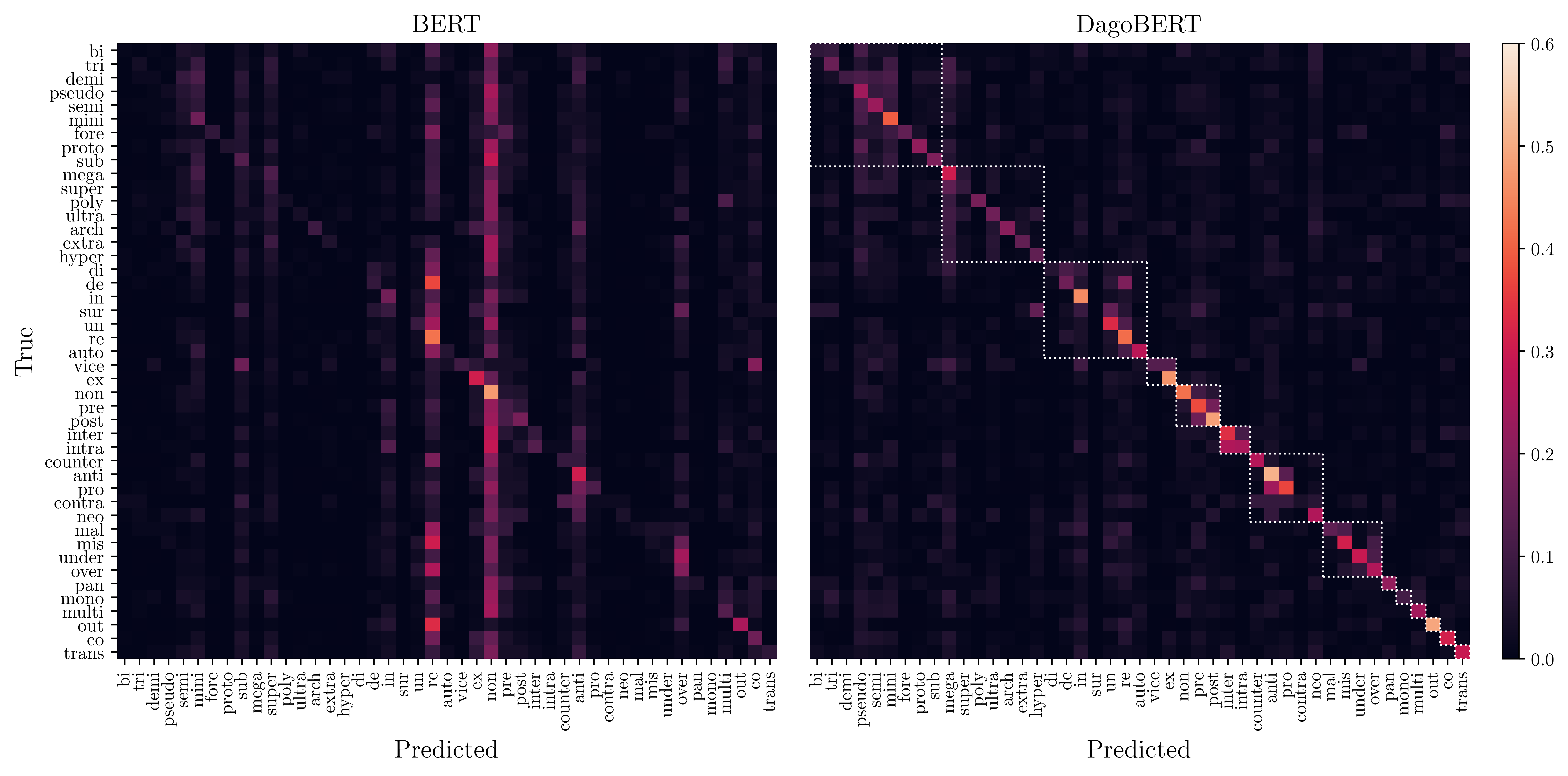
Figure 2: Prefixes predicted by BERT (left) and DagoBERT (right). Vertical lines indicate that a prefix has been overgenerated (particularly re and non in the left panel). The white boxes in the right panel highlight the clusters produced by Girvan-Newman after 4 graph splits.

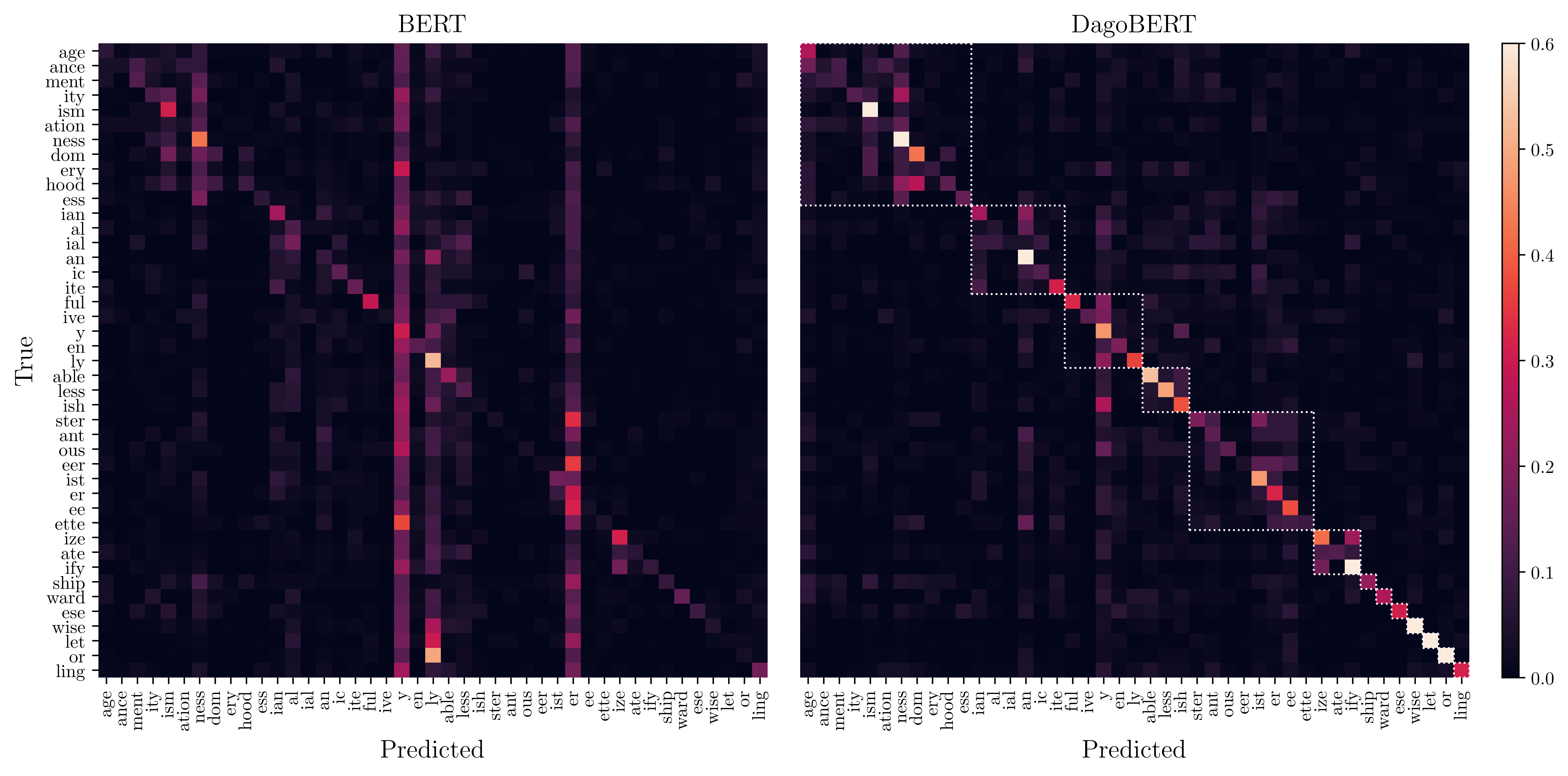
Figure 3: Suffixes predicted by pretrained BERT (left) and DagoBERT (right). Vertical lines indicate that a suffix has been overgenerated (particularly y, ly, and er in the left panel). The white boxes in the right panel highlight the clusters produced by Girvan-Newman after 4 graph splits.

5.2 Patterns of Confusion

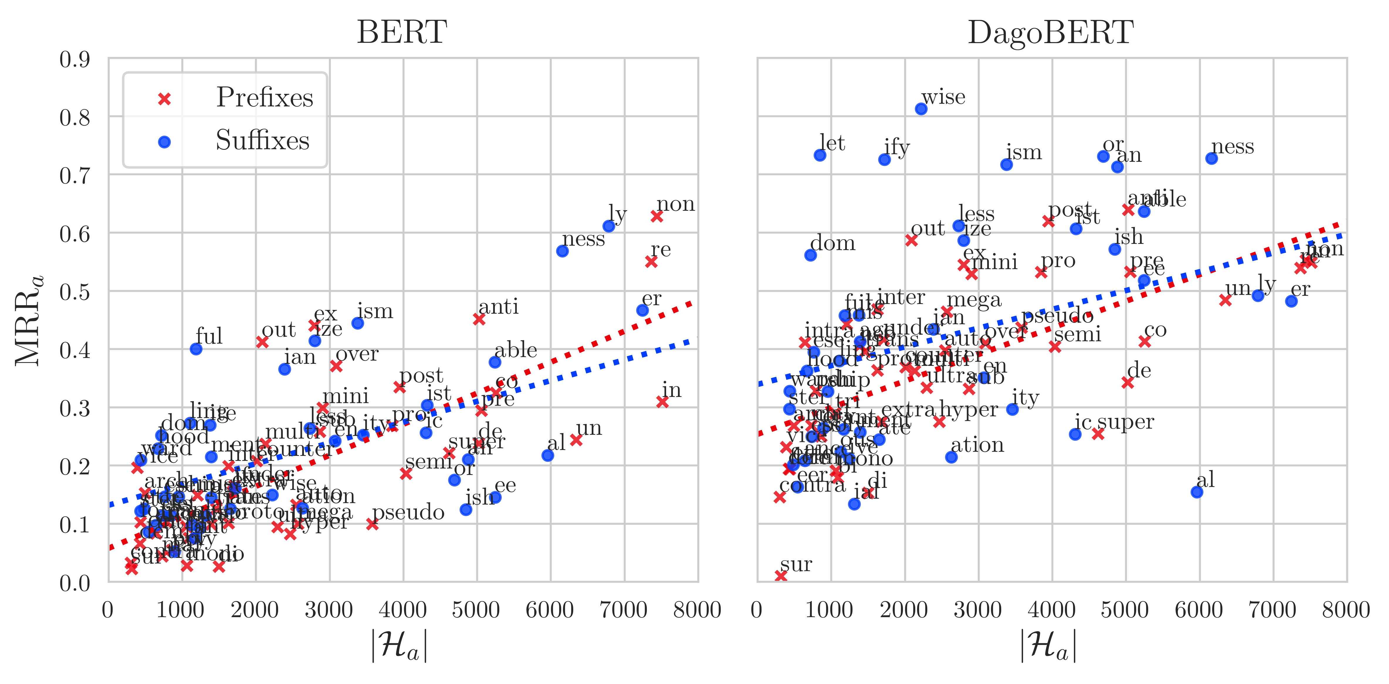
Figure 4: Correlation between number of hapaxes and MRR for pretrained BERT (left) and DagoBERT (right) on B1. The highly productive suffix y at $(12662,0.49)$ (left) and $(12662,0.62)$ (right) is not shown.

We now analyze in more detail the performance of the best performing model, DagoBERT, and contrast it with the performance of pretrained BERT. As a result of our definition of correct predictions (Section 4.1), the set of incorrect predictions is heterogeneous and potentially contains affixes resulting in equally possible derivatives. We are hence interested in patterns of confusion in the data.

We start by constructing the row-normalized confusion matrix $\mathbf{C}$ for the predictions of DagoBERT on the hapax derivatives (B1, SHARED) for P and S. Based on $\mathbf{C}$, we create a confusion graph $\mathcal{G}$ with adjacency matrix $\mathbf{G}$, whose elements are

$$G_{ij}=\bigl{\lceil}C_{ij}-\theta\bigr{\rceil},$$ (5)

i.e., there is a directed edge from affix $i$ to affix $j$ if $i$ was misclassified as $j$ with a probability greater than $\theta$. We set $\theta$ to 0.08. To uncover the community structure of $\mathcal{G}$, we use the Girvan-Newman algorithm (Girvan and Newman, 2002), which clusters the graph by iteratively removing the edge with the highest betweenness centrality.

The resulting clusters reflect linguistically interpretable groups of affixes (Table 8). In particular, the suffixes are clustered in groups with common POS. These results are confirmed by plotting the confusion matrix with an ordering of the affixes induced by all clusterings of the Girvan-Newman algorithm (Figure 2, Figure 3). They indicate that even when DagoBERT does not predict the affix occurring in the sentence, it tends to predict an affix semantically and syntactically congruent with the ground truth (e.g., ness for ity, ify for ize, inter for intra). In such cases, it is often a more productive affix that is predicted in lieu of a less productive one. Furthermore, DagoBERT frequently confuses affixes denoting points on the same scale, often antonyms (e.g., pro and anti, pre and post, under and over). This can be related to recent work showing that BERT has difficulties with negated expressions (Ettinger, 2020; Kassner and Schütze, 2020). Pretrained BERT shows similar confusion patterns overall but overgenerates several affixes much more strongly than DagoBERT, in particular re, non, y, ly, and er, which are among the most productive affixes in English (Plag, 1999, 2003).

To probe the impact of productivity more quantitatively, we measure the cardinality of the set of hapaxes formed by means of a particular affix $a$ in the entire dataset, $|\mathcal{H}_{a}|$, and calculate a linear regression to predict the MRR values of affixes based on $|\mathcal{H}_{a}|$. $|\mathcal{H}_{a}|$ is a common measure of morphological productivity (Baayen and Lieber, 1991; Pierrehumbert and Granell, 2018). This analysis shows a significant positive correlation for both prefixes ($R^{2}=.566$, $F(1,43)=56.05$, $p<.001$) and suffixes ($R^{2}=.410$, $F(1,41)=28.49$, $p<.001$): the more productive an affix, the higher its MRR value. This also holds for DagoBERT’s predictions of prefixes ($R^{2}=.423$, $F(1,43)=31.52$, $p<.001$) and suffixes ($R^{2}=.169$, $F(1,41)=8.34$, $p<.01$), but the correlation is weaker, particularly in the case of suffixes (Figure 4).

5.3 Impact of Input Segmentation

	FROZEN								FINETUNED
Segmentation	B1	B2	B3	B4	B5	B6	B7	$\mu\pm\sigma$	B1	B2	B3	B4	B5	B6	B7	$\mu\pm\sigma$
Morphological	.634	.645	.658	.675	.683	.692	.698	.669$\pm$.022	.762	.782	.797	.807	.800	.804	.799	.793$\pm$.015
WordPiece	.572	.578	.583	.590	.597	.608	.608	.591$\pm$.013	.739	.757	.766	.769	.767	.755	.753	.758$\pm$.010

Table 9: Performance (accuracy) of BERT on morphological well-formedness prediction with morphologically correct segmentation versus WordPiece tokenization. Best score per column in gray.

We have shown that BERT can generate derivatives if it is provided with the morphologically correct segmentation. At the same time, we observed that BERT’s WordPiece tokenizations are often morphologically incorrect, an observation that led us to impose the correct segmentation using hyphenation (HYP). We now examine more directly how BERT’s derivational knowledge is affected by using the original WordPiece segmentations versus the HYP segmentations.

We draw upon the same dataset as for DG (SPLIT) but perform binary instead of multi-class classification, i.e., the task is to predict whether, e.g., unwearable is a possible derivative in the context this jacket is           . or not. As negative examples, we combine the base of each derivative (e.g., wear) with a randomly chosen affix different from the original affix (e.g., ##ation) and keep the sentence context unchanged, resulting in a balanced dataset. We only use prefixed derivatives for this experiment.

We train binary classifiers using BERT_BASE and one of two input segmentations, the morphologically correct segmentation or BERT’s WordPiece tokenization. The BERT output embeddings for all subword units belonging to the derivative in question are max-pooled and fed into a dense layer with a sigmoid activation. We examine two settings: training only the dense layer while keeping BERT’s model weights frozen (FROZEN), or finetuning the entire model (FINETUNED). See Appendix A.3 for details about implementation, hyperparameter tuning, and runtime.

Morphologically correct segmentation consistently outperforms WordPiece tokenization, both on FROZEN and FINETUNED (Table 9). We interpret this in two ways. Firstly, the type of segmentation used by BERT impacts how much derivational knowledge can be learned, with positive effects of morphologically valid segmentations. Secondly, the fact that there is a performance gap even for models with frozen weights indicates that a morphologically invalid segmentation can blur the derivational knowledge that is in principle available and causes BERT to force semantically unrelated words to have similar representations. Taken together, these findings provide further evidence for the crucial importance of morphologically valid segmentation strategies in language model pretraining (Bostrom and Durrett, 2020).

6 Related Work

PLMs such as ELMo (Peters et al., 2018), GPT-2 (Radford et al., 2019), and BERT (Devlin et al., 2019) have been the focus of much recent work in NLP. Several studies have been devoted to the linguistic knowledge encoded by the parameters of PLMs (see Rogers et al. (2020) for a review), particularly syntax (Goldberg, 2019; Hewitt and Manning, 2019; Jawahar et al., 2019; Lin et al., 2019) and semantics (Ethayarajh, 2019; Wiedemann et al., 2019; Ettinger, 2020). There is also a recent study examining morphosyntactic information in a PLM, specifically BERT (Edmiston, 2020).

There has been relatively little recent work on derivational morphology in NLP. Both Cotterell et al. (2017) and Deutsch et al. (2018) propose neural architectures that represent derivational meanings as tags. More closely related to our study, Vylomova et al. (2017) develop an encoder-decoder model that uses the context sentence for predicting deverbal nouns. Hofmann et al. (2020b) propose a graph auto-encoder that models the morphological well-formedness of derivatives.

7 Conclusion

We show that a PLM, specifically BERT, can generate derivationally complex words. Our best model, DagoBERT, clearly beats an LSTM-based model, the previous state of the art in DG. DagoBERT’s errors are mainly due to syntactic and semantic overlap between affixes. Furthermore, we demonstrate that the input segmentation impacts how much derivational knowledge is available to BERT. This suggests that the performance of PLMs could be further improved if a morphologically informed vocabulary of units were used.

Appendix A Appendices

A.1 Data Preprocessing

We filter the posts for known bots and spammers Tan and Lee (2015). We exclude posts written in a language other than English and remove strings containing numbers, references to users, and hyperlinks. Sentences are filtered to contain between 10 and 100 words. We control that derivatives do not appear more than once in a sentence.

A.2 Hyperparameters

We tune hyperparameters on the development data separately for each frequency bin (selection criterion: MRR). Models are trained with categorical cross-entropy as the loss function and Adam (Kingma and Ba, 2015) as the optimizer. Training and testing are performed on a GeForce GTX 1080 Ti GPU (11GB).

DagoBERT. We use a batch size of 16 and perform grid search for the learning rate $l\in\{$1\text{\times}{10}^{-6}$,$3\text{\times}{10}^{-6}$,$1\text{\times}{10}^{-5}$,$3\text{\times}{10}^{-5}$\}$ and the number of epochs $n_{e}\in\{1,\dots,8\}$ (number of hyperparameter search trials: 32). All other hyperparameters are as for BERT_BASE. The number of trainable parameters is 110,104,890.

BERT+. We use a batch size of 16 and perform grid search for the learning rate $l\in\{$1\text{\times}{10}^{-4}$,$3\text{\times}{10}^{-4}$,$1\text{\times}{10}^{-3}$,$3\text{\times}{10}^{-3}$\}$ and the number of epochs $n_{e}\in\{1,\dots,8\}$ (number of hyperparameter search trials: 32). All other hyperparameters are as for BERT_BASE. The number of trainable parameters is 622,650.

LSTM. We initialize word embeddings with 300-dimensional GloVe (Pennington et al., 2014) vectors and character embeddings with 100-dimensional random vectors. The BiLSTMs consist of three layers and have a hidden size of 100. We use a batch size of 64 and perform grid search for the learning rate $l\in\{$1\text{\times}{10}^{-4}$,$3\text{\times}{10}^{-4}$,$1\text{\times}{10}^{-3}$,$3\text{\times}{10}^{-3}$\}$ and the number of epochs $n_{e}\in\{1,\dots,40\}$ (number of hyperparameter search trials: 160). The number of trainable parameters varies with the type of the model due to different sizes of the output layer and is 2,354,345 for P, 2,354,043 for S, and 2,542,038 for PS models.

Table 10 lists statistics of the validation performance over hyperparameter search trials and provides information about the best validation performance as well as corresponding hyperparameter configurations. We also report runtimes for the hyperparameter search.

For the models trained on the Vylomova et al. (2017) dataset, hyperparameter search is identical as for the main models, except that we use accuracy as the selection criterion. Runtimes for the hyperparameter search in minutes are 754 for SHARED and 756 for SPLIT in the case of DagoBERT, and 530 for SHARED and 526 for SPLIT in the case of LSTM. Best validation accuracy is .943 ($l=$3\text{\times}{10}^{-06}$$, $n_{e}=7$) for SHARED and .659 ($l=$1\text{\times}{10}^{-05}$$, $n_{e}=4$) for SPLIT in the case of DagoBERT, and .824 ($l=$1\text{\times}{10}^{-04}$$, $n_{e}=38$) for SHARED and .525 ($l=$1\text{\times}{10}^{-04}$$, $n_{e}=33$) for SPLIT in the case of LSTM.

A.3 Hyperparameters

We use the HYP segmentation method for models with morphologically correct segmentation. We tune hyperparameters on the development data separately for each frequency bin (selection criterion: accuracy). Models are trained with binary cross-entropy as the loss function and Adam as the optimizer. Training and testing are performed on a GeForce GTX 1080 Ti GPU (11GB).

For FROZEN, we use a batch size of 16 and perform grid search for the learning rate $l\in\{$1\text{\times}{10}^{-4}$,$3\text{\times}{10}^{-4}$,$1\text{\times}{10}^{-3}$,$3\text{\times}{10}^{-3}$\}$ and the number of epochs $n_{e}\in\{1,\dots,8\}$ (number of hyperparameter search trials: 32). The number of trainable parameters is 769. For FINETUNED, we use a batch size of 16 and perform grid search for the learning rate $l\in\{$1\text{\times}{10}^{-6}$,$3\text{\times}{10}^{-6}$,$1\text{\times}{10}^{-5}$,$3\text{\times}{10}^{-5}$\}$ and the number of epochs $n_{e}\in\{1,\dots,8\}$ (number of hyperparameter search trials: 32). The number of trainable parameters is 109,483,009. All other hyperparameters are as for BERT_BASE.

Table 11 lists statistics of the validation performance over hyperparameter search trials and provides information about the best validation performance as well as corresponding hyperparameter configurations. We also report runtimes for the hyperparameter search.

			SHARED							SPLIT
Model			B1	B2	B3	B4	B5	B6	B7	B1	B2	B3	B4	B5	B6	B7
DagoBERT	P	$\mu$	.349	.400	.506	.645	.777	.871	.930	.345	.364	.375	.383	.359	.359	.357
		$\sigma$	.020	.037	.096	.160	.154	.112	.064	.018	.018	.018	.019	.018	.017	.022
		$\max$	.372	.454	.657	.835	.896	.934	.957	.368	.385	.399	.412	.397	.405	.392
		$l$	1e-5	3e-5	3e-5	3e-5	1e-5	3e-6	3e-6	3e-6	1e-5	3e-6	1e-6	3e-6	1e-6	1e-6
		$n_{e}$	3	8	8	8	5	8	6	5	3	3	5	1	1	1
	S	$\mu$	.386	.453	.553	.682	.805	.903	.953	.396	.403	.395	.395	.366	.390	.370
		$\sigma$	.031	.058	.120	.167	.164	.118	.065	.033	.024	.020	.020	.019	.029	.027
		$\max$	.419	.535	.735	.872	.933	.965	.976	.429	.430	.420	.425	.403	.441	.432
		$l$	3e-5	3e-5	3e-5	3e-5	1e-5	1e-5	3e-6	3e-5	1e-5	3e-6	1e-6	1e-6	1e-6	1e-6
		$n_{e}$	2	7	8	6	8	7	6	2	3	5	7	3	2	1
	PS	$\mu$	.124	.214	.362	.554	.725	.840	.926	.119	.158	.175	.194	.237	.192	.176
		$\sigma$	.018	.075	.173	.251	.238	.187	.119	.013	.013	.011	.016	.020	.021	.018
		$\max$	.146	.337	.620	.830	.915	.945	.970	.135	.177	.192	.219	.269	.235	.209
		$l$	1e-5	3e-5	3e-5	3e-5	1e-5	3e-5	1e-5	1e-5	3e-6	3e-6	1e-6	1e-6	1e-6	1e-6
		$n_{e}$	6	8	8	5	8	3	7	6	8	3	4	4	1	1
		$\tau$	192	230	314	440	631	897	1,098	195	228	313	438	631	897	791
BERT+	P	$\mu$	.282	.336	.424	.527	.655	.764	.860	.280	.298	.318	.324	.323	.324	.322
		$\sigma$	.009	.020	.046	.078	.090	.080	.051	.011	.007	.009	.013	.009	.012	.009
		$\max$	.297	.374	.497	.633	.759	.841	.901	.293	.312	.334	.345	.341	.357	.346
		$l$	1e-4	1e-3	3e-3	1e-3	3e-4	3e-4	3e-4	1e-4	1e-4	1e-4	1e-4	1e-4	1e-4	1e-4
		$n_{e}$	7	8	8	8	8	8	8	5	8	7	2	4	1	1
	S	$\mu$	.358	.424	.491	.587	.708	.817	.886	.369	.364	.357	.350	.337	.335	.332
		$\sigma$	.010	.018	.043	.073	.086	.072	.049	.010	.010	.010	.013	.017	.017	.009
		$\max$	.372	.452	.557	.691	.806	.884	.925	.383	.377	.375	.372	.366	.377	.357
		$l$	1e-4	1e-3	1e-3	1e-3	1e-3	1e-3	3e-4	1e-4	1e-4	1e-4	1e-4	1e-4	1e-4	1e-4
		$n_{e}$	4	7	8	8	7	7	8	8	4	5	1	1	1	1
	PS	$\mu$	.084	.152	.257	.419	.598	.741	.849	.083	.104	.127	.137	.158	.139	.136
		$\sigma$	.008	.024	.062	.116	.119	.099	.062	.009	.014	.015	.014	.017	.011	.008
		$\max$	.099	.206	.371	.610	.756	.847	.913	.099	.131	.154	.170	.206	.173	.164
		$l$	1e-4	3e-3	3e-3	3e-3	1e-3	1e-3	1e-3	1e-4	1e-4	1e-4	1e-4	1e-4	1e-4	1e-4
		$n_{e}$	7	8	8	8	8	8	8	5	3	3	1	1	1	1
		$\tau$	81	102	140	197	285	406	568	80	101	140	196	283	400	563
LSTM	P	$\mu$	.103	.166	.314	.510	.661	.769	.841	.089	.113	.107	.106	.103	.103	.116
		$\sigma$	.031	.072	.163	.212	.203	.155	.107	.019	.024	.020	.017	.010	.010	.013
		$\max$	.159	.331	.583	.732	.818	.864	.909	.134	.152	.141	.138	.121	.120	.139
		$l$	1e-3	1e-3	1e-3	1e-3	3e-4	1e-4	3e-4	3e-4	3e-4	3e-4	3e-4	1e-4	1e-4	3e-4
		$n_{e}$	33	40	38	35	35	40	26	38	36	37	38	40	37	29
	S	$\mu$	.124	.209	.385	.573	.721	.824	.881	.108	.133	.136	.132	.132	.127	.128
		$\sigma$	.037	.098	.202	.229	.206	.162	.111	.029	.034	.027	.015	.013	.012	.012
		$\max$	.214	.422	.674	.812	.882	.925	.945	.192	.187	.179	.157	.159	.157	.153
		$l$	3e-4	1e-3	1e-3	1e-3	3e-4	3e-4	3e-4	3e-4	3e-4	3e-4	3e-4	3e-4	1e-4	1e-4
		$n_{e}$	40	40	37	31	37	38	39	37	38	37	39	38	39	29
	PS	$\mu$	.011	.066	.255	.481	.655	.776	.848	.009	.015	.025	.035	.046	.032	.071
		$\sigma$	.005	.090	.256	.301	.276	.220	.177	.003	.004	.006	.006	.008	.008	.015
		$\max$	.022	.346	.649	.786	.844	.886	.931	.016	.024	.038	.047	.065	.055	.104
		$l$	3e-3	3e-3	3e-3	3e-4	3e-4	3e-4	3e-4	3e-4	3e-3	3e-4	3e-4	3e-3	3e-3	3e-4
		$n_{e}$	38	40	39	40	33	40	39	40	39	23	32	28	15	31
		$\tau$	115	136	196	253	269	357	484	100	120	142	193	287	352	489

Table 10: Validation performance statistics and hyperparameter search details. The table shows the mean ($\mu$), standard deviation ($\sigma$), and maximum ($\max$) of the validation performance (MRR) on all hyperparameter search trials for prefix (P), suffix (S), and prefix-suffix (PS) models. It also gives the learning rate ($l$) and number of epochs ($n_{e}$) with the best validation performance as well as the runtime ($\tau$) in minutes averaged over P, S, and PS for one full hyperparameter search (32 trials for DagoBERT and BERT+, 160 trials for LSTM).

		FROZEN							FINETUNED
Segmentation		B1	B2	B3	B4	B5	B6	B7	B1	B2	B3	B4	B5	B6	B7
Morphological	$\mu$	.617	.639	.650	.660	.671	.684	.689	.732	.760	.764	.750	.720	.692	.657
	$\sigma$	.010	.009	.009	.008	.014	.009	.009	.016	.017	.029	.052	.067	.064	.066
	$\max$	.628	.649	.660	.669	.682	.692	.698	.750	.779	.793	.802	.803	.803	.808
	$l$	3e-4	3e-4	1e-4	1e-4	1e-4	1e-4	1e-4	1e-5	3e-6	3e-6	1e-6	1e-6	1e-6	1e-6
	$n_{e}$	8	5	7	7	5	3	5	4	8	5	8	3	2	1
	$\tau$	137	240	360	516	765	1,079	1,511	378	578	866	1,243	1,596	1,596	1,793
WordPiece	$\mu$	.554	.561	.569	.579	.584	.592	.596	.706	.730	.734	.712	.669	.637	.604
	$\sigma$	.011	.010	.011	.012	.011	.010	.011	.030	.021	.025	.052	.066	.061	.046
	$\max$	.568	.574	.582	.592	.597	.605	.608	.731	.752	.762	.765	.763	.759	.759
	$l$	1e-4	1e-4	1e-4	1e-4	1e-4	1e-4	1e-4	1e-5	3e-6	3e-6	1e-6	1e-6	1e-6	1e-6
	$n_{e}$	6	8	6	2	8	2	7	3	7	6	8	3	1	1
	$\tau$	139	242	362	517	765	1,076	1,507	379	575	869	1,240	1,597	1,598	1,775

Table 11: Validation performance statistics and hyperparameter search details. The table shows the mean ($\mu$), standard deviation ($\sigma$), and maximum ($\max$) of the validation performance (accuracy) on all hyperparameter search trials for classifiers using morphological and WordPiece segmentations. It also gives the learning rate ($l$) and number of epochs ($n_{e}$) with the best validation performance as well as the runtime ($\tau$) in minutes for one full hyperparameter search (32 trials for both morphological and WordPiece segmentations).

References

- Acquaviva (2016) Paolo Acquaviva. 2016. Morphological semantics. In Andrew Hippisley and Gregory Stump, editors, The Cambridge handbook of morphology, pages 117–148. Cambridge University Press, Cambridge.
- Apel and Lawrence (2011) Kenn Apel and Jessika Lawrence. 2011. Contributions of morphological awareness skills to word-level reading and spelling in first-grade children with and without speech sound disorder. Journal of Speech, Language, and Hearing Research, 54(5):1312–1327.
- Baayen and Lieber (1991) R. Harald Baayen and Rochelle Lieber. 1991. Productivity and English derivation: A corpus-based study. Linguistics, 29(5).
- Bauer (2001) Laurie Bauer. 2001. Morphological productivity. Cambridge University Press, Cambridge, UK.
- Bauer (2019) Laurie Bauer. 2019. Rethinking morphology. Edinburgh University Press, Edinburgh, UK.
- Bauer et al. (2013) Laurie Bauer, Rochelle Lieber, and Ingo Plag. 2013. The Oxford reference guide to English morphology. Oxford University Press, Oxford, UK.
- Bostrom and Durrett (2020) Kaj Bostrom and Greg Durrett. 2020. Byte pair encoding is suboptimal for language model pretraining. In arXiv 2004.03720.
- Brysbaert et al. (2016) Marc Brysbaert, Michaël Stevens, Paweł Mandera, and Emmanuel Keuleers. 2016. How many words do we know? practical estimates of vocabulary size dependent on word definition, the degree of language input and the participant’s age. Frontiers in Psychology, 7:1116.
- Cotterell et al. (2017) Ryan Cotterell, Ekaterina Vylomova, Huda Khayrallah, Christo Kirov, and David Yarowsky. 2017. Paradigm completion for derivational morphology. In Conference on Empirical Methods in Natural Language Processing (EMNLP) 2017.
- Crystal (1997) David Crystal. 1997. The Cambridge encyclopedia of the English language. Cambridge University Press, Cambridge, UK.
- Dal and Namer (2016) Georgette Dal and Fiammetta Namer. 2016. Productivity. In Andrew Hippisley and Gregory Stump, editors, The Cambridge handbook of morphology, pages 70–89. Cambridge University Press, Cambridge.
- Deutsch et al. (2018) Daniel Deutsch, John Hewitt, and Dan Roth. 2018. A distributional and orthographic aggregation model for English derivational morphology. In Annual Meeting of the Association for Computational Linguistics (ACL) 56.
- Devlin et al. (2019) Jacob Devlin, Ming-Wei Chang, Kenton Lee, and Kristina Toutanova. 2019. BERT: Pre-training of deep bidirectional transformers for language understanding. In Annual Conference of the North American Chapter of the Association for Computational Linguistics: Human Language Technologies (NAACL HTL) 17.
- Dodge et al. (2019) Jesse Dodge, Suchin Gururangan, Dallas Card, Roy Schwartz, and Noah A. Smith. 2019. Show your work: Improved reporting of experimental results. In Conference on Empirical Methods in Natural Language Processing (EMNLP) 2019.
- Edmiston (2020) Daniel Edmiston. 2020. A systematic analysis of morphological content in BERT models for multiple languages. In arXiv 2004.03032.
- Ethayarajh (2019) Kawin Ethayarajh. 2019. How contextual are contextualized word representations? comparing the geometry of BERT, ELMo, and GPT-2 embeddings. In Conference on Empirical Methods in Natural Language Processing (EMNLP) 2019.
- Ettinger (2020) Allyson Ettinger. 2020. What BERT is not: Lessons from a new suite of psycholinguistic diagnostics for language models. Transactions of the Association for Computational Linguistics, 8:34–48.
- Girvan and Newman (2002) Michelle Girvan and Mark Newman. 2002. Community structure in social and biological networks. Proceedings of the National Academy of Sciences of the United States of America, 99(12):7821–7826.
- Goldberg (2019) Yoav Goldberg. 2019. Assessing BERT’s syntactic abilities. In arXiv 1901.05287.
- ten Hacken (2014) Pius ten Hacken. 2014. Delineating derivation and inflection. In Rochelle Lieber and Pavol Štekauer, editors, The Oxford handbook of derivational morphology, pages 10–25. Oxford University Press, Oxford.
- Haspelmath and Sims (2010) Martin Haspelmath and Andrea D. Sims. 2010. Understanding morphology. Routledge, New York, NY.
- Hewitt and Manning (2019) John Hewitt and Christopher D. Manning. 2019. A structural probe for finding syntax in word representations. In Annual Conference of the North American Chapter of the Association for Computational Linguistics: Human Language Technologies (NAACL HTL) 17.
- Hofmann et al. (2020a) Valentin Hofmann, Janet B. Pierrehumbert, and Hinrich Schütze. 2020a. Predicting the growth of morphological families from social and linguistic factors. In Annual Meeting of the Association for Computational Linguistics (ACL) 58.
- Hofmann et al. (2020b) Valentin Hofmann, Hinrich Schütze, and Janet B. Pierrehumbert. 2020b. A graph auto-encoder model of derivational morphology. In Annual Meeting of the Association for Computational Linguistics (ACL) 58.
- Jawahar et al. (2019) Ganesh Jawahar, Benoit Sagot, and Djamé Seddah. 2019. What does BERT learn about the structure of language? In Annual Meeting of the Association for Computational Linguistics (ACL) 57.
- Kassner and Schütze (2020) Nora Kassner and Hinrich Schütze. 2020. Negated and misprimed probes for pretrained language models: Birds can talk, but cannot fly. In Annual Meeting of the Association for Computational Linguistics (ACL) 58.
- Kingma and Ba (2015) Diederik P. Kingma and Jimmy L. Ba. 2015. Adam: A method for stochastic optimization. In International Conference on Learning Representations (ICLR) 3.
- Lieber (2019) Rochelle Lieber. 2019. Theoretical issues in word formation. In Jenny Audring and Francesca Masini, editors, The Oxford handbook of morphological theory, pages 34–55. Oxford University Press, Oxford.
- Lin et al. (2019) Yongjie Lin, Yi C. Tan, and Robert Frank. 2019. Open sesame: Getting inside BERT’s linguistic knowledge. In Analyzing and Interpreting Neural Networks for NLP (BlackboxNLP) 2.
- Mahler et al. (2017) Taylor Mahler, Willy Cheung, Micha Elsner, David King, Marie-Catherine de Marneffe, Cory Shain, Symon Stevens-Guille, and Michael White. 2017. Breaking NLP: Using morphosyntax, semantics, pragmatics and world knowledge to fool sentiment analysis systems. In Workshop on Building Linguistically Generalizable NLP Systems 1.
- Pennington et al. (2014) Jeffrey Pennington, Richard Socher, and Christopher D. Manning. 2014. GloVe: Global vectors for word representation. In Conference on Empirical Methods in Natural Language Processing (EMNLP) 2014.
- Peters et al. (2018) Matthew Peters, Mark Neumann, Mohit Iyyer, Matt Gardner, Christopher Clark, Kenton Lee, and Luke Zettlemoyer. 2018. Deep contextualized word representations. In Annual Conference of the North American Chapter of the Association for Computational Linguistics: Human Language Technologies (NAACL HLT) 16.
- Pierrehumbert (2006) Janet B. Pierrehumbert. 2006. The statistical basis of an unnatural alternation. In Louis Goldstein, Douglas H. Whalen, and Catherine T. Best, editors, Laboratory Phonology 8, pages 81–106. De Gruyter, Berlin.
- Pierrehumbert and Granell (2018) Janet B. Pierrehumbert and Ramon Granell. 2018. On hapax legomena and morphological productivity. In Workshop on Computational Research in Phonetics, Phonology, and Morphology (SIGMORPHON) 15.
- Plag (1999) Ingo Plag. 1999. Morphological productivity: Structural constraints in English derivation. De Gruyter, Berlin.
- Plag (2003) Ingo Plag. 2003. Word-formation in English. Cambridge University Press, Cambridge, UK.
- Plag and Balling (2020) Ingo Plag and Laura W. Balling. 2020. Derivational morphology: An integrative perspective on some fundamental questions. In Vito Pirrelli, Ingo Plag, and Wolfgang U. Dressler, editors, Word knowledge and word usage: A cross-disciplinary guide to the mental lexicon, pages 295–335. De Gruyter, Berlin.
- Radev et al. (2002) Dragomir Radev, Hong Qi, Harris Wu, and Weiguo Fan. 2002. Evaluating web-based question answering systems. In International Conference on Language Resources and Evaluation (LREC) 3.
- Radford et al. (2019) Alec Radford, Jeffrey Wu, Rewon Child, David Luan, Dario Amodei, and Ilya Sutskever. 2019. Language models are unsupervised multitask learners.
- Rogers et al. (2020) Anna Rogers, Olga Kovaleva, and Anna Rumshisky. 2020. A primer in BERTology: What we know about how BERT works. In arXiv 2002.12327.
- Tan and Lee (2015) Chenhao Tan and Lillian Lee. 2015. All who wander: On the prevalence and characteristics of multi-community engagement. In International Conference on World Wide Web (WWW) 24.
- Vylomova et al. (2017) Ekaterina Vylomova, Ryan Cotterell, Timothy Baldwin, and Trevor Cohn. 2017. Context-aware prediction of derivational word-forms. In Conference of the European Chapter of the Association for Computational Linguistics (EACL) 15.
- Wiedemann et al. (2019) Gregor Wiedemann, Steffen Remus, Avi Chawla, and Chris Biemann. 2019. Does BERT make any sense? interpretable word sense disambiguation with contextualized embeddings. In arXiv 1909.10430.
- Wu et al. (2016) Yonghui Wu, Mike Schuster, Zhifeng Chen, Quoc Le V, Mohammad Norouzi, Wolfgang Macherey, Maxim Krikun, Yuan Cao, Qin Gao, Klaus Macherey, Jeff Klingner, Apurva Shah, Melvin Johnson, Xiaobing Liu, Łukasz Kaiser, Stephan Gouws, Yoshikiyo Kato, Taku Kudo, Hideto Kazawa, Keith Stevens, George Kurian, Nishant Patil, Wei Wang, Cliff Young, Jason Smith, Jason Riesa, Alex Rudnick, Oriol Vinyals, Greg Corrado, Macduff Hughes, and Jeffrey Dean. 2016. Google’s neural machine translation system: Bridging the gap between human and machine translation. In arXiv 1609.08144.
- Yang et al. (2019) Zhilin Yang, Zihang Dai, Yiming Yang, Jaime Carbonell, Ruslan Salakhutdinov, and Quoc V. Le. 2019. XLNet: Generalized autoregressive pretraining for language understanding. In Advances in Neural Information Processing Systems (NeurIPS) 33.