Stochastic Neighbor Embedding of Multimodal Relational Data
for Image-Text Simultaneous Visualization

Abstract

Multimodal relational data analysis has become of increasing importance in recent years, for exploring across different domains of data, such as images and their text tags obtained from social networking services (e.g., Flickr). A variety of data analysis methods have been developed for visualization; to give an example, $t$-Stochastic Neighbor Embedding ($t$-SNE) computes low-dimensional feature vectors so that their similarities keep those of the observed data vectors. However, $t$-SNE is designed only for a single domain of data but not for multimodal data; this paper aims at visualizing multimodal relational data consisting of data vectors in multiple domains with relations across these vectors. By extending $t$-SNE, we herein propose Multimodal Relational Stochastic Neighbor Embedding (MR-SNE), that (1) first computes augmented relations, where we observe the relations across domains and compute those within each of domains via the observed data vectors, and (2) jointly embeds the augmented relations to a low-dimensional space. Through visualization of Flickr and Animal with Attributes 2 datasets, proposed MR-SNE is compared with other graph embedding-based approaches; MR-SNE demonstrates the promising performance.

1 Introduction

Many different types of data called multimodal data (i.e., text, image, and audio) has become readily available over recent years, by virtue of the rapid development of information technology. The data type is especially called domain or view, and analyzing the relations across different domains has attracted extensive attention (Davidson et al.,, 2010; Sharma et al.,, 2012; Hong et al.,, 2014; Mathew et al.,, 2016; Chu and Tsai,, 2017).

As can be easily assumed from the surrounding environment of image processing, datasets employed recently comprise high-dimensional data vectors and their complicated relations. For instance, images and their relevant texts have complicated graph-structured relations, as several texts are simultaneously associated with each of the images. Such a relation across domains is characterized by an across-domains graph; data vectors in each domain and the across-domains graph are together called multimodal relational data.

However, these data vectors are perplexing to comprehend by humans due to their high-dimensionality. Thus data visualization has an indispensable role in delving into the observed relational data, as it converts the perplexing high-dimensional data vectors into the corresponding low-dimensional vectors that are easily comprehensible to humans. Their underlying relations within and across domains are then expected to be identified with external human knowledge.

One of the most popular approaches for visualization in recent years is $t$-stochastic neighbor embedding ($t$-SNE; Maaten and Hinton,, 2008), that first computes similarities between all pairs of the data vectors, where they are especially called stochastic neighbor graph, and it subsequently computes the low-dimensional vectors so that their graph is preserved. $t$-SNE is classified into manifold learning (Belkin and Niyogi,, 2003; Cayton,, 2005; Talwalkar et al.,, 2008), which is well developed so far. However, manifold learning requires defining similarities between data vectors; $t$-SNE cannot be applied to multimodal data, that contains data vectors whose different dimensionalities depend on the domain.

Although $t$-SNE cannot be directly applied, there have been a variety of alternatives for visualizing multimodal relational data. One way is to employ cross-domain matching correlation analysis (CDMCA; Shimodaira,, 2016, Figure 1(a)), which incorporates graph embedding into linear canonical correlation analysis (CCA; Harold,, 1936) so that the low-dimensional vectors represent observed graph-structured relations. Probabilistic multi-view graph embedding (PMvGE; Okuno et al.,, 2018) employs highly expressive neural networks for transforming data vectors to low-dimensional feature vectors. PMvGE predicts an underlying relation via similarity between the pair of obtained feature vectors, which may provide a good visualization. In our link prediction experiment across domains, PMvGE using inner-product similarity and squared Euclidean distance demonstrate a better ROC-AUC score than CDMCA and random prediction.

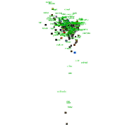
(a) CDMCA (0.657)

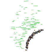
(b) PMvGE (0.811)
Inner-Product

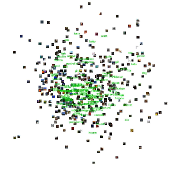
(c) PMvGE (0.884)
Squared-Distance

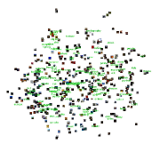
(d) MR-SNE (0.828)
Proposal

Figure 1: An observed graph across text and image domains in the Flickr dataset is embedded into a $2$-dim. subspace. ROC-AUC scores for link prediction across domains are provided in parentheses (higher is better). Note that the existing $t$-SNE is not listed here as it cannot be applied to the multimodal relational data. See Section 4 for further details.

However, PMvGE with only the observed across-domains graph does not fully leverage the underlying but unobserved relations within each of domains, that are also crucial for visualization; its visualization can be unsatisfactory in several practical cases. For instance, Figure 1(b) shows that the text and image feature vectors obtained via PMvGE with inner-product similarity are completely separated, even though it shows a good ROC-AUC score for link prediction across domains. Mimno and Thompson, (2017) reported the same phenomenon in skip-gram (Mikolov et al.,, 2013) (a.k.a. word2vec), that similarly considers only a graph across word and context domains. Figure 1(c) shows that text vectors are unnaturally concentrated around the center when squared Euclidean distance is employed.

Therefore, this paper extends $t$-SNE to the multimodal setting, so that not only the observed across-domains graph but also stochastic neighbor graphs computed within each domain are considered, as shown in Figure 2.

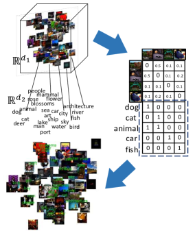
Figure 2: Proposed MR-SNE: Observed across-domains graph and stochastic neighbor graphs computed within each of domains are jointly embedded into the common subspace, by applying $t$-SNE framework.

Our contribution: We propose Multimodal Relational Stochastic Neighbor Embedding (MR-SNE), that (i) first computes stochastic neighbor graphs within each domain so that they predict the underlying but unobserved relations, (ii) computes augmented relations for the multimodal relational data, by linking up the observed across-domains graph and the stochastic neighbor graphs computed within each of domains, and (iii) jointly embeds the augmented relations by applying the existing $t$-SNE framework. The proposed MR-SNE extends $t$-SNE to the multimodal setting, and it provides a good visualization, as shown in Figure 3. Extensive numerical experiments are conducted through visualization of Flicker and Animal with Attributes 2 (AwA2) dataset; other possible approaches for visualizing multimodal relational data are also empirically compared with the proposed MR-SNE.

Organization of this paper: problem setting is summarized in Section 2, proposed MR-SNE is described in Section 3, numerical experiments are conducted in Section 4, and Section 5 concludes this paper.

1.1 Related Works

Laplacian eigenmaps (Belkin and Niyogi,, 2003), multidimensional scaling (MDS; Torgerson,, 1952) and Isomap (Tenenbaum et al.,, 2000) are manifold learning methods; they cannot be applied to multimodal data, similarly to $t$-SNE (Maaten and Hinton,, 2008) and principal component analysis (PCA; Pearson,, 1901). Multi-view SNE (m-SNE; Xie et al.,, 2011) considers vector representations of objects in $2$ domains, indicating their $2$ different perspectives; the objects therein are essentially $1$-view, and m-SNE consequently provides one vector representation for each object by aggregating these $2$-domains. Thus the problem setting is different from this paper. One-to-one relations across $2$ domains and stochastic neighbor graphs computed within each of $2$ domains are simultaneously considered in Quadrianto and Lampert, (2011), Sun and Chen, (2007), Zhao and Evans-Dugelay Zhao et al., (2013) and Wang and Zhang, (2013), but they cannot be applied to multimodal relational data.

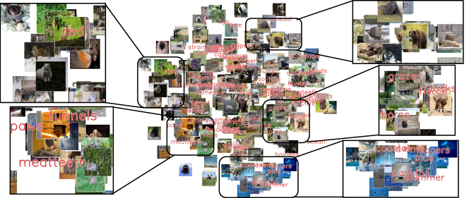
Figure 3: Simultaneous visualization of $n_{1}=2500$ images and their $n_{2}=85$ text tags in Animal with Attributes 2 dataset (Xian et al.,, 2018). Randomly selected 500 images are shown here. The data vectors are $d_{1}=2048$ dim. CNN image vectors $\{x^{(1)}_{i}\}_{i=1}^{n_{1}}$ and $d_{2}=300$ dim. GloVe word vectors $\{x^{(2)}_{j}\}_{j=1}^{n_{2}}$. These data vectors are embedded in $K=2$-dim. common subspace, by applying the proposed MR-SNE. See Fig. 7 in Supplementary Material B for Flickr dataset.

2 Problem Setting

In this section, we describe the problem setting when $D=2$ domains are considered. It can be straightforwardly generalized to arbitrary $D\geq 1$.

Let $d_{1},d_{2},n_{1},n_{2}\in\mathbb{N}$ and let $\{x_{i}^{(1)}\}_{i=1}^{n_{1}}\subset\mathbb{R}^{d_{1}},\{x_{j}^{(2)}\}_{j=1}^{n_{2}}\subset\mathbb{R}^{d_{2}}$ be data vectors for the two domains. $W=(w_{ij})\in\mathbb{R}_{\geq 0}^{n_{1}\times n_{2}}$ is the observed across-domains graph; $w_{ij}\geq 0$ represents the strength of relation between $x^{(1)}_{i}\in\mathbb{R}^{d_{1}}$ and $x^{(2)}_{j}\in\mathbb{R}^{d_{2}}$, where $w_{ij}=0$ represents no relation. Then, our goal is to provide a better visualization of the multimodal relational data $(\{x^{(1)}_{i}\}_{i=1}^{n_{1}},\{x^{(2)}_{j}\}_{j=1}^{n_{2}},\{w_{ij}\}_{i,j=1}^{n_{1},n_{2}})$, by transforming $d_{1},d_{2}$-dimensional data vectors in each domain into the user-specified $K(\leq\min\{d_{1},d_{2}\})$-dimensional feature vectors $\{y_{i}^{(1)}\}_{i=1}^{n_{1}},\{y_{j}^{(2)}\}_{j=1}^{n_{2}}\subset\mathbb{R}^{K}$. Particularly, $K=2$ is considered for visualization.

A typical example is the simultaneous visualization of images and their text tags, which is shown in Figure 3. In this example, (i) data vectors for images $\{x_{i}^{(1)}\}_{i=1}^{n_{1}}\subset\mathbb{R}^{d_{1}}$ and their text tags $\{x^{(2)}_{j}\}_{j=1}^{n_{2}}\subset\mathbb{R}^{d_{2}}$, and (ii) relations $\{w_{ij}\}_{i,j=1}^{n_{1},n_{2}}$ across image and text domains, are observed; $w_{ij}=1$ indicates that the image $i$ is tagged with the text $j$ and $w_{ij}=0$ otherwise.

Current issue is that the conventional $t$-SNE cannot be applied to multimodal relational data, whose dimensions $d_{1},d_{2}$ of $2$ domains are different, as it requires measuring Euclidean distance between data vectors. For instance, considering the case that $d_{1}=10,d_{2}=20$, Euclidean distance between $x^{(1)}_{i}\in\mathbb{R}^{10},x^{(2)}_{j}\in\mathbb{R}^{20}$ is not well-defined.

3 Proposed Method

In this section, we propose an extension of $t$-SNE, that can be applied to multimodal relational data. Stochastic neighbor graph is defined in Section 3.1, and the proposed method is described in Section 3.2. Although the case of $D=2$ domains is considered, it can be straightforwardly extended to general $D\geq 1$; $D=1$ corresponds to the conventional $t$-SNE.

3.1 Stochastic neighbor Graph Within Each Domain

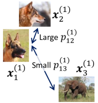
Figure 4: $p^{(1)}_{ij}$ is computed depending on the distance between vectors.

In this section, we explain the stochastic neighbor graph within each domain, that is defined in Maaten and Hinton, (2008) for the case $D=1$. Firstly, let us think of the graph for domain $1$.

Conditional probability for each pair $(x^{(1)}_{i},x^{(1)}_{j})$ is defined as

$$p_{j|i}^{(1)} =\scalebox{0.85}{$\displaystyle\frac{{\rm exp}(-\|x^{(1)}_{i}-x^{(1)}_{j}\|_{2}^{2}/2s^{2}_{i})}{\sum_{k\neq i}\ \exp(-\|x^{(1)}_{i}-x^{(1)}_{k}\|_{2}^{2}/2s^{2}_{i})}$},$$ (1)

where $s_{i}>0\>(i=1,2,\ldots,n_{1})$ are user-specified parameters. In Maaten and Hinton, (2008), the parameters $\{s_{i}\}_{i=1}^{n_{1}}$ are determined by (i) specifying only one parameter $\lambda>0$ called “perplexity”, and (ii) solving equations $\lambda=2^{H_{i}}$ with $H_{i}:=-\sum_{j}p^{(1)}_{j\mid i}\log p^{(1)}_{j\mid i}$, for $i=1,2,\ldots,n$. Using (1), pairwise similarity is defined as $p^{(1)}_{ij}:=(p^{(1)}_{i\mid j}+p^{(1)}_{j\mid i})/2n_{1}$ for $i\neq j$ and $p^{(1)}_{ii}=0$; stochastic Neighbor graph is defined as $P^{(1)}=(p^{(1)}_{ij})$. $t$-SNE regards each entry $p^{(1)}_{ij}$ as a joint probability of the pair $(x^{(1)}_{i},x^{(1)}_{j})$, as $\{p^{(1)}_{ij}\}$ are non-negative and their total sum is $1$. The graph $P^{(2)}$ for domain $2$ is similarly defined.

3.2 Proposed Method

In this section, we propose Multimodal Relational Stochastic Neighbor Embedding (MR-SNE) that visualizes the multimodal relational data, as shown in Figure 2; the procedure is formally defined in the following (i)-(iii), and is also shown in Algorithm 1 in Supplement A.

1. Stochastic neighbor graphs $P^{(1)}=(p_{ij}^{(1)})\in\mathbb{R}_{\geq 0}^{n_{1}\times n_{1}},P^{(2)}=(p_{ij}^{(2)})\in\mathbb{R}_{\geq 0}^{n_{2}\times n_{2}}$ for each domain $1,2$ are computed as explained in Section 3.1.

2. Observed across-domains graph $W=(w_{ij})\in\mathbb{R}^{n_{1}\times n_{2}}_{\geq 0}$ is normalized to $r_{ij}=\frac{w_{ij}}{\sum_{i=1}^{n_{1}}\sum_{j=1}^{n_{2}}w_{ij}}$. $r_{ij}$ is regarded as the joint probability of the pair of $2$ domain vectors $(x^{(1)}_{i},x^{(2)}_{j})$. We denote the normalized across-domains graph by $R=(r_{ij})\in\mathbb{R}^{n_{1}\times n_{2}}_{\geq 0}$.

3. We construct a matrix $\tilde{P}\in\mathbb{R}_{\geq 0}^{(n_{1}+n_{2})\times(n_{1}+n_{2})}$ from the above matrices $P^{(1)},P^{(2)},R$ as

   $$\tilde{P}:=\scalebox{0.85}{$\displaystyle\left(\begin{array}[]{cc}\beta_{1}P^{(1)}&\frac{\beta_{12}}{2}R\\ \frac{\beta_{12}}{2}R^{\top}&\beta_{2}P^{(2)}\\ \end{array}\right)$},$$ (4)

   where $\beta_{1},\beta_{12},\beta_{2}\geq 0$ are user-specified parameters satisfying a constraint $\beta_{1}+\beta_{12}+\beta_{2}=1$. Then, we regard the entries in $\tilde{P}$ as a joint probability of the corresponding data vectors, as all the entries are non-negative and their total sum is $1$.

4. We consider the corresponding low-dimensional feature vectors $\{y^{(1)}_{i}\}_{i=1}^{n_{1}},\{y^{(2)}_{i}\}_{i=1}^{n_{2}}\subset\mathbb{R}^{K}$, and define a joint probability of $(y^{(d)}_{i},y^{(e)}_{j})$ for $i\in[n_{d}],j\in[n_{e}],d,e\in[2]$ by

   $$q^{(d,e)}_{ij}=\scalebox{0.85}{$\displaystyle\frac{(1+\|y^{(d)}_{i}-y^{(e)}_{j}\|_{2}^{2})^{-1}}{\sum_{(f,k)}\sum_{(g,l)\neq(f,k)}(1+\|y^{(f)}_{k}-y^{(g)}_{l}\|_{2}^{2})^{-1}}\quad(\text{if }(d,i)\neq(e,j))$},$$ (5)

   and $q^{(d,d)}_{ii}=0$. We construct a matrix $\tilde{Q}\in\mathbb{R}_{\geq 0}^{(n_{1}+n_{2})\times(n_{1}+n_{2})}$ from the matrices $Q^{(1)}=(q^{(1,1)}_{ij}),Q^{(2)}=(q^{(2,2)}_{ij}),Q^{(1,2)}=(q^{(1,2)}_{ij})$ as

   $$\tilde{Q}:=\scalebox{0.85}{$\displaystyle\left(\begin{array}[]{cc}Q^{(1)}&Q^{(1,2)}\\ (Q^{(1,2)})^{\top}&Q^{(2)}\\ \end{array}\right)$}.$$ (8)

5. Low-dimensional vectors $\{y^{(1)}_{i}\}_{i=1}^{n_{1}},\{y^{(2)}_{i}\}_{i=1}^{n_{2}}\subset\mathbb{R}^{K}$ are consequently computed by minimizing the Kullback-Leibler divergence between the two distributions $\tilde{P},\tilde{Q}$, that is

   $$\tilde{C} =\text{KL}(\tilde{P}||\tilde{Q})=\sum_{d=1}^{2}\beta_{d}\underbrace{\scalebox{0.85}{$\displaystyle\sum_{i=1}^{n_{d}}\sum_{j=1}^{n_{d}}p^{(d)}_{ij}\log\frac{p^{(d)}_{ij}}{q^{(d,d)}_{ij}}$}}_{\text{within each domain}}+\beta_{12}\underbrace{\scalebox{0.85}{$\displaystyle\sum_{i=1}^{n_{1}}\sum_{j=1}^{n_{2}}r_{ij}\log\frac{r_{ij}}{q^{(1,2)}_{ij}}$}}_{\text{across domains}}+\text{Const.},$$ (9)

   where $\beta_{1},\beta_{12},\beta_{2}\geq 0$ are parameters specified in (4). In practice, we employ full-batch gradient descent (Rumelhart et al.,, 1987) with momentum, to optimize the objective function (9).

4 Numerical Experiments

In this section, we conduct numerical experiments on visualizing $2$-domain data vectors of images and their text tags, in the $(K=)2$-dimensional common subspace.

• Datasets: We employ two datasets consisting of $n_{1}$ images, $n_{2}$ text tags, and their graph across domains $W=(w_{ij})\in\mathbb{R}^{n_{1}\times n_{2}}_{\geq 0}$. $w_{ij}=1$ represents that the text $j$ is tagged with the image $i$, and $w_{ij}=0$ otherwise. Within-domain graphs are not observed.

  • For Flickr dataset (Thomee et al.,, 2016), $n_{1}=1000$ images are picked up at random, and the most frequently appeared $n_{2}=613$ text tags are selected. $d_{1}=2048$-dimensional image vectors are computed by CNN using ImageNet (Szegedy et al.,, 2016). We here employ $1$-hot vectors for representing text tags, i.e., $y^{(2)}_{j}\in\{0,1\}^{n_{2}}$ whose $j$-th entry is $1$ and $0$ otherwise; distributed representations of words, such as word2vec (Mikolov et al.,, 2013), may be employed instead.

  • For Animal with Attributes 2 (AwA2) dataset (Xian et al.,, 2018), we employ $n_{1}=2500$ images consisting of 50 images for each of 50 classes, and their associated $n_{2}=85$ text tags. $d_{1}=2048$-dimensional image vectors are computed by ResNet (He et al.,, 2016), and $d_{2}=300$-dimensional word vectors are computed by GloVe (Pennington et al.,, 2014).

• Baselines: The following methods are compared to the proposed MR-SNE.

  • CDMCA (Shimodaira,, 2016) extends linear CCA (Harold,, 1936) so that across-domains graph $W=(w_{ij})$ is considered. Kernel CDMCA incorporates Gaussian kernel into CDMCA. They both are also regularized. See Supplement F for details.

  • PMvGE (Okuno et al.,, 2018) computes feature vectors $y^{(d)}_{i}:=f^{(d)}_{\theta}(x^{(d)}_{i})\in\mathbb{R}^{K}$ via neural networks $f^{(d)}_{\theta}:\mathbb{R}^{p_{d}}\to\mathbb{R}^{K}$ for each domain $d=1,2$, by maximizing the likelihood using a model $w_{ij}\overset{\text{indep.}}{\sim}\text{B}(\sigma(-s(y^{(1)}_{i},y^{(2)}_{j})))$. $\text{B}(\mu)$ represents Bernoulli distribution whose expectation is $\mu\in[0,1]$, and $\sigma(z):=(1+\exp(z))^{-1}$. Although arbitrary $s:\mathbb{R}^{2K}\to\mathbb{R}$ can be used, $s(y,y^{\prime}):=\|y-y^{\prime}\|_{2}^{2}$ is here considered; see Figure 1 for visualization with inner-product $s(y,y^{\prime})=-\langle y,y^{\prime}\rangle$.

• Preprocessing: the following options are considered.

  • For CDMCA / Kernel CDMCA / PMvGE: (ignored) unobserved within-domain graphs $W^{(1)},W^{(2)}$ are not considered as usual.

  • For PMvGE: (2nd-order) $\hat{W}^{(1)}=W^{\top}W,\hat{W}^{(2)}=WW^{\top}$ called 2nd-order proximity (see, e.g., Tang et al., (2015)) are alternatively employed for domain $1,2$.

  • For the proposed MR-SNE, the across-domains graph $W$ is (unnorm) used without normalization, (norm) normalized as $\frac{w_{ij}}{\sqrt{\sum_{k\neq i}w_{ik}}\sqrt{\sum_{l\neq j}w_{lj}}}$, (PMI) normalized as $\frac{w_{ij}}{\sum_{k\neq i}w_{ik}\sum_{l\neq j}w_{lj}}$ similarly to Point-wise Mutual Information (Church and Hanks,, 1990).

• Training: The proposed model is trained by fullbatch gradient descent summarized in Algorithm 1 in Supplement A, with the number of iterations $T=500$, learning rate $\eta=100$ and momentum $\alpha=0.5$. Also see Supplement A.1 for computational time. PMvGE is trained by minibatch SGD with negative sampling, that is used in a variety of existing researches, such as word2vec (Mikolov et al.,, 2013), LINE (Tang et al.,, 2015).

4.1 Experiment 1: Visualization

Flickr and AwA2 datasets are visualized in the following Figures 6 and 6, respectively. These plots show 500 images randomly selected from the $n_{1}$ images. Also, the 120 most frequently used tags in Flickr and all 85 tags in AwA2 are displayed in green.

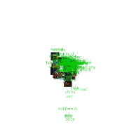
(a) CDMCA

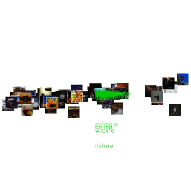
(b) Kernel CDMCA

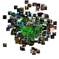
(c) PMvGE (ignored)

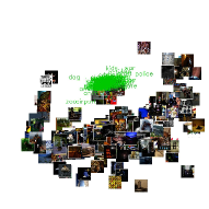
(d) PMvGE (2nd-order)

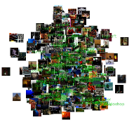
(e) Proposal
($\beta_{1}=\beta_{12}=1/2,\beta_{2}=0)$

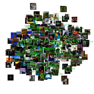
(f) Proposal ($\beta_{1}\propto n_{1}^{2}$,
$\beta_{12}\propto n_{1}n_{2},\beta_{2}=0$)

Figure 5: Visualization of Flickr dataset

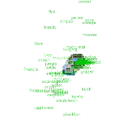
(a) PMvGE (ignored)

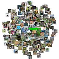
(b) Proposal
($\beta_{1}=\beta_{12}=\beta_{2}=1/3)$

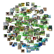
(c) Proposal ($\beta_{1}\propto n_{1}^{2}$,
$\beta_{12}\propto n_{1}n_{2},\beta_{2}\propto n_{2}^{2}$)

Figure 6: Visualization of AwA2 dataset

Results: (i) Feature vectors obtained in CDMCA (Fig. 5(a)) and kernel CDMCA (Fig. 5(b)) are unnaturally concentrated at the center in Flickr experiment. (ii) PMvGE that does not leverage within-domain graphs, i.e., PMvGE using only the across-domains graph, provides appropriate visualization for Flickr dataset (Fig. 5(c)), but not for AwA2 dataset (Fig. 6(a)). (iii) Text vectors computed via PMvGE with 2nd-order proximity are improperly shrinked for Flickr visualization (Fig. 5(d)). (iv) The proposed MR-SNE provides good visualization for both Flickr and AwA2 datasets (Fig. 5(e), 5(f), 6(b), 6(c)); See Figure 3 for more detailed visualization. Above methods including the proposed MR-SNE are numerically evaluated in the following Section 4.2 and 4.3.

4.2 Experiment 2: Graph Reconstruction

Using Flickr and AwA2 dataset, the proposed MR-SNE and other baselines are evaluated by ROC-AUC score for graph reconstruction, that is defined as follows: (i) for each query image, nearest $k$ images or text tags are predicted to be linked, (ii) ROC-AUC score (Bradley,, 1997) with respect to $k=1,2,\ldots,n_{1}+n_{2}-1$ is subsequently computed for Flickr ($k=1,2,\ldots,1612$) and AwA2 ($k=1,2,\ldots,2584$). Therefore, this experiment considers reconstructing both within-domain and across-domains graph, though only the across-domains graph can be leveraged for training. Higher ROC-AUC score is better; scores for Flickr and AwA2 datasets are listed in the following Table 7(a) and 7(b), respectively. ROC curves for these experiments are also shown in Supplement C.

Table 1: ROC-AUC score for graph reconstruction. For $K>2$, $t$-SNE is applied to obtain $2$-dim. vectors. Best score is bolded and the second best is underlined.

		ignored / unnorm	2nd-order / norm	PMI
CDMCA	$(K=2)$	0.5022	/	/
	$(K=200)$	0.6112	/	/
	$(K=613)$	0.5707	/	/
K-CDMCA	$(K=2)$	0.4902	/	/
	$(K=200)$	0.5428	/	/
	$(K=613)$	0.5445	/	/
PMvGE	($K=2$)	0.7482	0.7918	/
	$(K=100)$	0.7111	0.7778	/
MR-SNE	($\beta_{1}=\beta_{12}=1,\beta_{2}=0$)	0.7134	0.7038	0.6690
	( $\beta_{1}=\frac{n_{1}^{2}}{n_{1}^{2}+n_{1}n_{2}},\beta_{2}=0,\beta_{12}=\frac{n_{1}n_{2}}{n_{1}^{2}+n_{1}n_{2}}$ )	0.7000	0.6902	0.6542

(a) Flickr dataset

		ignored / unnorm	2nd-order / norm	PMI
CDMCA	$(K=2)$	0.5650	/	/
	$(K=200)$	0.6506	/	/
	$(K=613)$	0.6439	/	/
K-CDMCA	$(K=2)$	0.6427	/	/
	$(K=200)$	0.7283	/	/
	$(K=613)$	0.7285	/	/
PMvGE	($K=2$)	0.6576	0.3517	/
	$(K=100)$	0.3682	0.3657	/
MR-SNE	($\beta_{1}=\beta_{2}=\beta_{12}=1$)	0.7117	0.7161	0.7109
	( $\beta_{d}=\frac{n_{d}^{2}}{n_{1}^{2}+n_{2}^{2}+n_{1}n_{2}},\beta_{12}=\frac{n_{1}n_{2}}{n_{1}^{2}+n_{2}^{2}+n_{1}n_{2}}$ )	0.8033	0.8124	0.8134

(b) AwA2 dataset

Interpretation: Overall, the proposed MR-SNE outperforms the existing CDMCA and Kernel-CDMCA. So we here mainly consider comparing the proposed MR-SNE to existing highly non-linear PMvGE. Firstly, Table 7(a) indicates that PMvGE demonstrates higher ROC-AUC score than others for Flickr dataset; the proposed MR-SNE is next to PMvGE. Unlike the Flickr dataset consisting of $n_{1}=1000$ images and $n_{2}=613$ text tags, AwA2 dataset contains $n_{1}=2500$ images and much fewer $n_{2}=85$ text tags; the numbers are disproportionate. In the AwA2 dataset, PMvGE demonstrates the worst performance whereas the proposed MR-SNE demonstrates the highest score therein. Thus the proposed MR-SNE is only a method that demonstrates promising performance for both of these two datasets.

4.3 Experiment 3: Variance of Feature Vectors for Different Domains

Whereas ROC-AUC score for graph reconstruction is considered in the previous Section 4.2, we hereinafter examine whether the obtained feature vectors for both domains are not shrinked improperly, by computing their variance. In this experiment, we first compute the sample variance-covariance matrices $\hat{\Sigma}^{(\text{image})},\hat{\Sigma}^{(\text{text})}\in\mathbb{R}^{2\times 2}$ for sets of data vectors $\mathcal{Y}^{(\text{image})}:=\{y_{i}^{(\text{image})}\}_{i=1}^{n_{1}},\mathcal{Y}^{(\text{text})}:=\{y_{j}^{(\text{text})}\}_{j=1}^{n_{2}}$, respectively. Subsequently, $r:=\frac{\text{tr}\hat{\Sigma}^{(\text{image})}}{\text{tr}\hat{\Sigma}^{(\text{text})}}$ is computed for each of datasets in Table 2 below, where $\text{tr}A=\sum_{i=1}^{d}a_{ii}$ denotes trace of $A=(a_{ij})$.

		ignored / unnorm	2nd-order / norm	PMI
PMvGE	$(K=2)$	1.448	1.666	/
	$(K=100)$	1.192	0.719	/
MR-SNE	($\beta_{1}=\beta_{12}=1,\beta_{2}=0$)	1.706	1.388	1.151
	( $\beta_{1}=\frac{n_{1}^{2}}{n_{1}^{2}+n_{1}n_{2}},\beta_{2}=0,\beta_{12}=\frac{n_{1}n_{2}}{n_{1}^{2}+n_{1}n_{2}}$ )	1.556	1.475	1.067

(c) Flickr dataset

		ignored / unnorm	2nd-order / norm	PMI
PMvGE	$(K=2)$	0.031	0.001	/
	$(K=100)$	0.170	0.282	/
MR-SNE	($\beta_{1}=\beta_{2}=\beta_{12}=1$)	56.563	26.139	27.800
	( $\beta_{d}=\frac{n_{d}^{2}}{n_{1}^{2}+n_{2}^{2}+n_{1}n_{2}},\beta_{12}=\frac{n_{1}n_{2}}{n_{1}^{2}+n_{2}^{2}+n_{1}n_{2}}$ )	1.087	1.190	1.165

(d) AwA2 dataset

Table 2: $r:=\frac{\text{tr}\hat{\Sigma}^{(\text{image})}}{\text{tr}\hat{\Sigma}^{(\text{text})}}$ is listed; $t$-SNE is applied to obtain $2$-dimensional vectors for $K>2$.

Interpretation: Roughly speaking, the vectors are improperly shrinked if $r$ is far away from the value $1$. For instance, PMvGE ($K=2$) using $2$nd-order proximity leads to $r=0.001$, indicating that $\text{tr}\hat{\Sigma}^{(\text{image})}$ is much smaller than $\text{tr}\hat{\Sigma}^{(\text{text})}$. Image vectors are then obviously improperly shrinked. On the other hand, MR-SNE with the adaptive weights satisfies $r\approx 1$ for both of datasets; MR-SNE is more stable than the existing PMvGE.

4.4 Additional Numerical Experiments

Additional numerical experiments are also conducted in Supplement D. Overall, the proposed MR-SNE demonstrates better score than other baselines for $K=2$; thus MR-SNE is expected to provide better visualization. Also see Supplement E for PMvGE equipped with stochastic neighbor graph.

5 Conclusion and Future Works

We proposed MR-SNE, that visualizes multimodal relational data, such as images, texts, and their relations in Flickr (Thomee et al.,, 2016) and AwA2 (Xian et al.,, 2018) datasets. MR-SNE (i) first computes augmented relations for the multimodal relational data, where the relations across domains are observed and those within domains are computed via the observed data vectors, and (2) jointly embeds the multimodal relational data to a common low-dimensional subspace. Numerical experiments were conducted for performing MR-SNE and other alternatives for visualizing multimodal relational data. For future work, it would be worthwhile to (i) consider more efficient computation of MR-SNE by referring to a multi-core extension of $t$-SNE (van der Maaten,, 2014; Ulyanov,, 2016), and (ii) develop more effective metric for evaluating visualization methods.

Appendix A Algorithm

The following Algorithm 1 describes the optimization procedure of the proposed MR-SNE, that is also explained in Section 3.2.

Algorithm 1 Multimodal Relational Stochastic Neighbor Embedding ($D=2$).

0:  Data vectors $\{x^{(1)}_{i}\}^{n_{1}}_{i=1}\in\mathbb{R}^{d_{1}}$, $\{x^{(2)}_{j}\}^{n_{2}}_{j=1}\in\mathbb{R}^{d_{2}}$, across-domains graph $W=(w_{ij})\in\mathbb{R}^{n_{1}\times n_{2}}$, and dimensionality $K$ of the common subspace.For cost function: perplexity $\lambda>0$, weights $\beta_{1},\beta_{2},\beta_{12}\geq 0$ satisfying $\beta_{1}+\beta_{2}+\beta_{12}=1$. For optimization: number of iterations $T\in\mathbb{N}$, initial learning rate $\eta>0$, momentum $\alpha>0$.

0:  Low-dimensional vectors $\{y^{(1)}_{i}\}_{i=1}^{n_{1}},\{y^{(2)}_{j}\}_{j=1}^{n_{2}}\subset\mathbb{R}^{K}$.

  Parameters $\{\sigma_{i}\}_{i=1}^{n}$ are computed via the user-specified perplexity.

  Compute stochastic neighbor graphs $P^{(1)},P^{(2)}$ and the normalized across-domains graph $R$ by the step (i) in Section 3.2; subsequently construct the matrix $\tilde{P}$ from the matrices $P^{(1)},P^{(2)},R$.

  Randomly initialize the entries in $Y=(y^{(1)}_{1},y^{(1)}_{2},\ldots,y^{(1)}_{n_{1}},y^{(2)}_{1},y^{(2)}_{2},\ldots,y^{(2)}_{n_{2}})$ with the normal distribution $N(0,10^{-4})$, and set $Y^{(0)}=Y^{(1)}$.

  for $t=1$ to $T$ do

     Compute $\tilde{Q}$ by the step (ii) in Section 3.2.

     Update $Y^{(t)}$ by leveraging the full-batch gradient descent with momentum:

$$Y^{(t+1)}=Y^{(t)}-\eta_{t}\frac{\partial\tilde{C}}{\partial Y^{(t)}}+\alpha_{t}(Y^{(t)}-Y^{(t-1)}),$$ (10)

where $\tilde{C}$ is defined in eq. (9).

     Multiply $1/10$ to the learning rate for each $400$ iterations: $\eta_{t+1}=\eta_{t}/10$ for $t=400k\>(k\in\mathbb{N})$ and $\eta_{t+1}=\eta_{t}$ otherwise. The momentum is kept fixed as $\alpha_{t}=\alpha$ in our implementation.

  end for

  Output $Y^{(T+1)}$.

A.1 Computational time

Numerical experiments were performed on a server with (CPU) 3.70 GHz Intel Xeon E5-1620 v2 and (GPU) NVIDIA GP102 TITAN Xp. The computation time was roughly $8$ hours and $11.5$ hours for training MR-SNE on the Flickr and AwA2 datasets, respectively. In this this study, we did not attempt an efficient implementation of MR-SNE, and it would be a future work to consider more efficient computation by referring to a multi-core extension of $t$-SNE (van der Maaten,, 2014; Ulyanov,, 2016).

Appendix B Visualization of Flickr dataset

Similarly to Figure 3 of AwA2 dataset, visualization of Flickr dataset is shown in Figure 7.

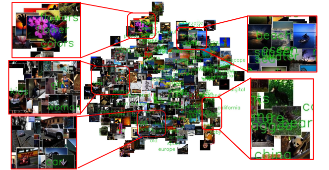
Figure 7: Simultaneous visualization of $n_{1}=1000$ images and most frequently appeared $n_{2}=613$ text tags in Flickr dataset. Randomly selected 500 images and the 120 most frequently used tags are displayed in green. These vectors are embedded in $K=2$ dimensional common subspace, by applying the proposed MR-SNE.

Appendix C ROC-Curve

In Experiment 2 shown in Section 4.2, proposed MR-SNE is compared to the baselines by ROC-AUC score for the task of graph reconstruction. ROC curve is shown in Figure 8, for each of Flickr and AwA2 datasets. In these plots, “MR-SNE (weight + …)” represents that the weights $\beta_{1},\beta_{2},\beta_{12}$ therein are specified by $\beta_{1}=\frac{n_{1}^{2}}{n_{1}^{2}+n_{1}n_{2}},\beta_{2}=0,\beta_{12}=\frac{n_{1}n_{2}}{n_{1}^{2}+n_{1}n_{2}}$ for Flickr dataset and $\beta_{d}=\frac{n_{d}^{2}}{n_{1}^{2}+n_{2}^{2}+n_{1}n_{2}},\beta_{12}=\frac{n_{1}n_{2}}{n_{1}^{2}+n_{2}^{2}+n_{1}n_{2}}$ for AwA2 dataset.

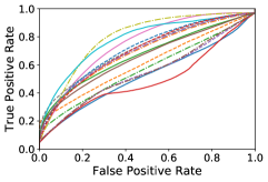
(a) Flickr

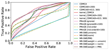
(b) AwA2

Figure 8: ROC-curve

Appendix D Additional Numerical Experiments

In addition to Experiment 1–3 shown in Section 4.1–4.3, the proposed MR-SNE and other baselines are here evaluated by the following four evaluation metrics, that are also shown in Figure 9. Amongst all the evaluations, $k$-nearest neighbors are computed via the obtained feature vectors in the common subspace.

1. Metric (I) across domains: For each query image, we examine whether at least one associated text tag is in its $k$-nearest neighbor text tags (searched over all the text tags); we then compute the proportion of such queries to all the query images.

2. Metric (I) within image domain: For each query image, we examine whether at least one image in its $k$-nearest neighbor (searched over all the images) shares at least one text tag with the query; we then compute the proportion of such queries to all the query images.

3. Metric (II) across domains: For each query image, we compute the number of associated text tags in its $k$-nearest neighbor text tags (searched over all the text tags); the numbers are also averaged over all the query images.

4. Metric (II) within image domain: For each query image, we compute the number of images sharing at least one text tag with the query, in its $k$-nearest neighbor images (searched over all the images); the numbers are also averaged over all the query images.

Higher score is better; scores for Flickr and AwA2 datasets are listed in the following Table 310(a)–610(h). In these tables, “MR-SNE (weight + …)” represents that $\beta_{1},\beta_{2},\beta_{12}$ are specified as defined in Supplement C.

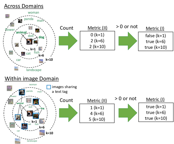
Figure 9: Four metrics used in supplementary numerical experiments. For a image query (dog), we compute the scores: the scores are averaged over all the queries.

D.1 Metric (I) across domains

Table 3: Evaluated by metric (I) across domains. For $K>2$, $t$-SNE is applied to obtain $2$-dim. vectors. Best score is bolded and the second best is underlined.

		$k=$1	2	5	10	20	50	100	200	500
CDMCA	($K=2$)	0.021	0.042	0.085	0.141	0.221	0.382	0.531	0.707	0.912
	($K=200$)	0.758	0.808	0.843	0.852	0.871	0.891	0.909	0.923	0.949
	($K=613$)	0.806	0.821	0.838	0.856	0.884	0.929	0.944	0.952	0.955
K-CDMCA	($K=2$)	0.024	0.030	0.062	0.121	0.229	0.379	0.517	0.665	0.888
	($K=200$)	0.046	0.056	0.103	0.143	0209	0.365	0.503	0.706	0.912
	($K=613$)	0.059	0.064	0.102	0.166	0.253	0.384	0.523	0.684	0.917
PMvGE-ignored	($K=2$)	0.078	0.136	0.263	0.414	0.629	0.837	0.928	0.952	0.955
	($K=100$)	0.544	0.651	0.763	0.824	0.871	0.908	0.940	0.952	0.955
PMvGE-2nd-order	($K=2$)	0.015	0.074	0.196	0.371	0.569	0.805	0.895	0.943	0.955
	($K=100$)	0.035	0.040	0.050	0.075	0.127	0.210	0.315	0.538	0.920
MR-SNE	(unnorm)	0.163	0.280	0.464	0.632	0.774	0.870	0.904	0.930	0.952
	(norm)	0.234	0.363	0.578	0.733	0.848	0.926	0.942	0.949	0.955
	(PMI)	0.319	0.485	0.729	0.844	0.905	0.938	0.943	0.952	0.955
	(weight+unnorm)	0.163	0.258	0.458	0.621	0.741	0.848	0.889	0.925	0.950
	(weight+norm)	0.208	0.349	0.568	0.725	0.829	0.902	0.930	0.946	0.954
	(weight+PMI)	0.313	0.462	0.674	0.809	0.889	0.927	0.942	0.948	0.954

(a) Flickr dataset

		$k=$1	2	3	5	10	20	30	50
CDMCA	($K=2$)	0.579	0.798	0.893	0.970	0.994	0.999	1.000	1.000
	($K=200$)	0.246	0.502	0.635	0.798	0.939	1.000	1.000	1.000
	($K=300$)	0.264	0.539	0.718	0.858	0.995	1.000	1.000	1.000
K-CDMCA	($K=2$)	0.576	0.754	0.843	0.962	1.000	1.000	1.000	1.000
	($K=200$)	0.174	0.490	0.713	0.874	0.952	0.986	1.000	1.000
	($K=300$)	0.192	0.497	0.704	0.855	0.955	0.986	1.000	1.000
PMvGE-ignored	($K=2$)	0.698	0.887	0.948	0.988	0.999	1.000	1.000	1.000
	($K=100$)	0.140	0.220	0.540	0.720	0.904	0.924	0.944	1.000
PMvGE-2nd-order	($K=2$)	0.685	0.950	0.997	1.000	1.000	1.000	1.000	1.000
	($K=100$)	0.100	0.180	0.180	0.800	0.974	1.000	1.000	1.000
MR-SNE	(unnorm)	0.539	0.756	0.804	0.923	0.984	0.999	1.000	1.000
	(norm)	0.232	0.389	0.669	0.798	0.906	0.987	1.000	1.000
	(PMI)	0.128	0.291	0.389	0.516	0.712	0.947	0.999	1.000
	(weight+unnorm)	0.520	0.751	0.863	0.919	0.995	0.999	1.000	1.000
	(weight+norm)	0.620	0.758	0.824	0.925	0.997	1.000	1.000	1.000
	(weight+PMI)	0.703	0.841	0.881	0.961	0.995	0.999	1.000	1.000

(b) AwA2 dataset

Overall, CDMCA ($K=613$) demonstrates better scores in Flickr dataset. However, the good scores are for $K=613$, meaning that the dimension of feature vector is very high; when considering only the case $K=2$, that is usually used for visualization, MR-SNE (PMI) demonstrates the best performance. Thus MR-SNE is expected for providing better visualization. For AwA2 dataset, PMI-2nd ($K=2$) demonstrates the best scores. Overall, $K=2$ is better than $K>2$ amongst all the baselines; only the low-dimension is required for representing associations across domains, for AwA2 dataset.

D.2 Metric (I) within image domain

Table 4: Evaluated by metric (I) within image domain. For $K>2$, $t$-SNE is applied to obtain $2$-dim. vectors. Best score is bolded and the second best is underlined.

		$k=$1	2	5	10	20	50	100	200	500
CDMCA	($K=2$)	0.170	0.272	0.421	0.522	0.634	0.760	0.838	0.903	0.950
	($K=200$)	0.887	0.904	0.913	0.926	0.939	0.944	0.947	0.949	0.953
	($K=613$)	0.643	0.722	0.790	0.841	0.884	0.918	0.937	0.948	0.955
K-CDMCA	($K=2$)	0.094	0.169	0.329	0.511	0.655	0.809	0.876	0.925	0.949
	($K=200$)	0.191	0.280	0.441	0.566	0.699	0.809	0.874	0.915	0.944
	($K=613$)	0.194	0.291	0.434	0.550	0.677	0.805	0.870	0.922	0.946
PMvGE-ignored	($K=2$)	0.213	0.337	0.536	0.700	0.819	0.917	0.949	0.955	0.955
	($K=100$)	0.640	0.762	0.874	0.911	0.938	0.948	0.954	0.955	0.955
PMvGE-2nd-order	($K=2$)	0.210	0.322	0.529	0.664	0.787	0.881	0.929	0.949	0.955
	($K=100$)	0.641	0.758	0.852	0.896	0.922	0.941	0.946	0.950	0.953
MR-SNE	(unnorm)	0.266	0.409	0.602	0.731	0.821	0.897	0.923	0.939	0.951
	(norm)	0.296	0.450	0.689	0.806	0.888	0.935	0.949	0.951	0.954
	(PMI)	0.329	0.514	0.742	0.864	0.919	0.950	0.953	0.953	0.955
	(weight+unnorm)	0.262	0.386	0.584	0.708	0.805	0.889	0.916	0.935	0.951
	(weight+norm)	0.283	0.438	0.656	0.779	0.863	0.923	0.942	0.951	0.955
	(weight+PMI)	0.343	0.487	0.690	0.826	0.900	0.941	0.950	0.954	0.955

(c) Flickr dataset

		$k=$1	2	5	10	20	50	100	200	500	1000
CDMCA	($K=2$)	0.124	0.162	0.259	0.376	0.541	0.787	0.919	0.978	0.996	1.000
	($K=200$)	0.721	0.773	0.820	0.849	0.872	0.917	0.945	0.969	0.991	1.000
	($K=300$)	0.730	0.787	0.837	0.859	0.887	0.916	0.947	0.970	0.992	0.999
K-CDMCA	($K=2$)	0.170	0.242	0.388	0.546	0.724	0.892	0.960	0.991	0.998	1.000
	($K=200$)	0.647	0.736	0.831	0.874	0.906	0.941	0.966	0.986	0.996	0.999
	($K=300$)	0.661	0.748	0.833	0.877	0.904	0.942	0.967	0.986	0.996	1.000
PMvGE-ignored	($K=2$)	0.088	0.157	0.299	0.461	0.656	0.865	0.950	0.985	0.999	1.000
	($K=100$)	0.038	0.058	0.059	0.060	0.060	0.080	0.100	0.140	0.260	0.460
PMvGE-2nd-order	($K=2$)	0.027	0.051	0.131	0.235	0.393	0.676	0.863	0.974	1.000	1.000
	($K=100$)	0.096	0.156	0.252	0.380	0.549	0.790	0.918	0.979	0.997	1.000
MR-SNE	(unnorm)	0.553	0.638	0.728	0.777	0.831	0.888	0.934	0.964	0.989	0.998
	(norm)	0.540	0.612	0.701	0.760	0.810	0.880	0.929	0.964	0.993	0.998
	(PMI)	0.560	0.642	0.727	0.784	0.828	0.893	0.936	0.968	0.989	0.999
	(weight+unnorm)	0.767	0.837	0.899	0.924	0.940	0.958	0.972	0.982	0.994	0.999
	(weight+norm)	0.775	0.847	0.904	0.925	0.944	0.963	0.975	0.986	0.993	0.998
	(weight+PMI)	0.758	0.837	0.892	0.918	0.936	0.956	0.972	0.984	0.992	0.998

(d) AwA2 dataset

Observation is almost similar to the evaluation by metric (I) across domains. For both datasets, overall, MR-SNE demonstrates higher scores than other methods if $K=2$; MR-SNE is expected for providing better visualization. If $K>2$, PMvGE demonstrates higher scores than others for Flickr dataset, whereas MR-SNE does for AwA2.

D.3 Metric (II) across domains

Table 5: Evaluated by metric (II) across domains. For $K>2$, $t$-SNE is applied to obtain $2$-dim. vectors. Best score is bolded and the second best is underlined.

		$k=$1	2	5	10	20	50	100	200	500
CDMCA	($K=2$)	0.021	0.048	0.118	0.227	0.392	0.765	1.236	2.078	4.233
	($K=200$)	0.758	1.212	1.599	1.694	1.798	2.081	2.538	3.322	5.090
	($K=613$)	0.806	1.050	1.135	1.222	1.346	1.743	2.297	3.449	5.338
K-CDMCA	($K=2$)	0.024	0.033	0.071	0.151	0.359	0.780	1.214	1.916	3.967
	($K=200$)	0.046	0.074	0.147	0.217	0.321	0.648	1.099	2.075	4.503
	($K=613$)	0.059	0.087	0.160	0.260	0.423	0.776	1.312	2.171	4.616
PMvGE-ignored	($K=2$)	0.078	0.142	0.328	0.584	1.067	2.283	3.672	4.959	5.551
	($K=100$)	0.544	0.865	1.357	1.758	2.173	2.823	3.467	4.323	5.470
PMvGE-2nd-order	($K=2$)	0.015	0.075	0.243	0.549	1.066	1.978	2.858	3.880	5.382
	($K=100$)	0.035	0.046	0.061	0.103	0.210	0.384	0.652	1.293	4.867
MR-SNE	(unnorm)	0.163	0.311	0.646	1.066	1.663	2.713	3.634	4.590	5.417
	(norm)	0.234	0.426	0.801	1.286	1.873	2.855	3.597	4.425	5.429
	(PMI)	0.319	0.549	1.069	1.519	2.045	2.784	3.361	4.069	5.296
	(weight+unnorm)	0.163	0.294	0.637	1.081	1.690	2.726	3.591	4.459	5.400
	(weight+norm)	0.208	0.395	0.819	1.247	1.822	2.737	3.472	4.289	5.385
	(weight+PMI)	0.313	0.546	0.967	1.378	1.839	2.503	3.142	3.918	5.282

(e) Flickr dataset

		$k=$1	2	3	5	10	20	30	50
CDMCA	($K=2$)	0.579	1.142	1.728	2.892	5.766	11.169	16.257	24.929
	($K=200$)	0.246	0.591	0.855	1.491	3.340	7.269	10.922	18.555
	($K=300$)	0.264	0.636	0.973	1.582	3.110	6.849	10.906	19.327
K-CDMCA	($K=2$)	0.576	1.146	1.541	2.438	4.706	8.812	12.109	19.620
	($K=200$)	0.174	0.563	1.064	1.650	3.528	7.281	11.254	19.222
	($K=300$)	0.192	0.597	1.052	1.646	3.520	7.156	11.255	19.267
PMvGE-ignored	($K=2$)	0.697	1.387	2.072	3.366	6.786	13.547	19.505	26.720
	($K=100$)	0.140	0.240	0.660	1.280	2.545	4.686	6.493	14.005
PMvGE-2nd-order	($K=2$)	0.685	1.442	2.298	3.272	6.694	12.583	18.077	26.386
	($K=100$)	0.100	0.220	0.240	1.120	2.298	6.520	10.794	20.900
MR-SNE	(unnorm)	0.539	1.116	1.542	2.515	4.783	8.991	13.232	20.397
	(norm)	0.232	0.523	1.022	1.866	3.657	7.636	11.901	20.972
	(PMI)	0.128	0.368	0.637	1.216	2.690	6.245	11.663	22.029
	(weight+unnorm)	0.520	1.078	1.640	2.606	5.122	10.943	16.841	25.017
	(weight+norm)	0.620	1.150	1.536	2.463	4.982	9.883	15.232	24.361
	(weight+PMI)	0.703	1.301	1.902	2.979	5.766	10.462	14.266	21.985

(f) AwA2 dataset

Amongst all the methods with $K=2$, for Flickr dataset, MR-SNE demonstrates the best score for $k\leq 50$, whereas PMvGE (ignored) is the best for $k>50$; thus MR-SNE outperforms PMvGE (ignored) depending on the dataset. However, on the other hand, for AwA2 dataset, PMvGE (ignored) shows better performance than others for $K=2$. For $K>2$, PMvGE and CDMCA outperform MR-SNE, whereas increasing $K>2$ does not improve the scores for AwA2 dataset.

D.4 Metric (II) within image domain

Table 6: Evaluated by metric (II) within image domain. For $K>2$, $t$-SNE is applied to obtain $2$-dim. vectors. Best score is bolded and the second best is underlined.

		$k=$1	2	5	10	20	50	100	200	500
CDMCA	($K=2$)	0.170	0.359	0.902	1.726	3.392	7.965	14.842	26.061	47.934
	($K=200$)	0.887	1.688	3.453	4.801	6.102	8.941	13.375	21.465	42.486
	($K=613$)	0.643	1.033	1.556	2.230	3.380	6.405	11.029	19.172	40.605
K-CDMCA	($K=2$)	0.094	0.186	0.458	0.931	1.844	4.556	8.906	17.528	43.205
	($K=200$)	0.191	0.338	0.760	1.358	2.458	5.138	9.361	17.967	42.529
	($K=613$)	0.194	0.355	0.774	1.357	2.388	5.142	9.468	18.181	42.710
PMvGE-ignored	($K=2$)	0.213	0.405	0.954	1.843	3.685	8.947	16.960	31.457	62.299
	($K=100$)	0.640	1.192	2.563	4.287	6.852	12.690	19.875	31.230	56.989
PMvGE-2nd-order	($K=2$)	0.210	0.393	0.961	1.943	3.806	9.311	18.334	35.087	68.956
	($K=100$)	0.641	1.147	2.389	3.963	6.685	13.637	23.434	37.873	65.739
MR-SNE	(unnorm)	0.266	0.549	0.954	1.843	3.685	8.947	16.960	31.457	62.299
	(norm)	0.296	0.581	1.414	2.721	5.045	11.036	19.525	32.592	59.104
	(PMI)	0.329	0.664	1.552	2.873	5.085	10.471	17.700	28.494	51.905
	(weight+unnorm)	0.262	0.497	1.233	2.424	4.640	10.791	19.479	33.216	60.680
	(weight+norm)	0.283	0.558	1.350	2.544	4.775	10.461	18.302	30.544	56.870
	(weight+PMI)	0.343	0.643	1.460	2.665	4.705	9.532	15.950	26.055	50.217

(g) Flickr dataset

		$k=$1	2	5	10	20	50	100	200	500	1000
CDMCA	($K=2$)	0.124	0.178	0.312	0.548	1.020	2.4052	4.562	8.338	17.577	28.845
	($K=200$)	0.721	1.360	3.105	5.794	10.696	21.044	26.800	30.992	36.768	42.002
	($K=300$)	0.730	1.400	3.258	6.109	11.202	22.010	28.050	32.106	37.954	42.546
K-CDMCA	($K=2$)	0.170	0.270	0.554	1.003	1.788	3.702	6.210	9.869	17.610	27.447
	($K=200$)	0.647	1.188	2.486	4.070	6.018	9.304	12.810	17.692	26.788	36.288
	($K=300$)	0.661	1.218	2.546	4.181	6.130	9.384	12.755	17.562	26.443	35.956
PMvGE-ignored	($K=2$)	0.088	0.184	0.443	0.854	1.661	3.808	7.110	12.761	24.470	36.839
	($K=100$)	0.038	0.074	0.182	0.364	0.726	1.797	2.895	4.855	10.735	20.535
PMvGE-2nd-order	($K=2$)	0.027	0.051	0.139	0.264	0.517	1.258	2.517	4.952	11.763	22.279
	($K=100$)	0.096	0.192	0.458	0.844	1.497	3.030	4.937	7.599	14.563	24.318
MR-SNE	(unnorm)	0.553	1.013	2.278	4.221	7.673	14.724	18.703	21.747	26.868	32.510
	(norm)	0.540	0.997	2.259	4.208	7.750	14.870	18.344	21.349	26.351	32.016
	(PMI)	0.560	1.047	2.396	4.481	8.102	15.326	19.503	22.623	26.829	32.067
	(weight+unnorm)	0.767	1.483	3.532	6.824	13.063	27.188	33.363	36.922	40.957	44.492
	(weight+norm)	0.775	1.492	3.560	6.878	13.227	27.998	34.212	37.498	40.739	43.966
	(weight+PMI)	0.758	1.472	3.502	6.777	12.948	27.621	34.212	37.804	40.872	43.866

(h) AwA2 dataset

For AwA2 dataset, overall, MR-SNE ourperforms all the other methods, including those for $K>2$; thus MR-SNE is expected to provide good visualization. For Flickr dataset, MR-SNE shows the best score for $K=2$, whereas PMvGE outperforms MR-SNE for $K>2$. This is also the same observation as the experiments in Supplement D.1.

Appendix E PMvGE using Stochastic Neighbor Graph

Similarly to the proposed MR-SNE, we may consider employing stochastic neighbor (SN) graph for PMvGE. Although such an augmented PMvGE using SN graph is not included in the original PMvGE, meaning that this extension may not be included in baselines, we here perform this augmented PMvGE to be compared with MR-SNE.

For training the PMvGE, we sampled $10^{5}$ edges with probabilities depending on the SN graph, that we call as “positive” edges; using a graph consisting of the sampled edges, we optimize PMvGE using negative sampling. Then, Flickr and AwA2 datasets are visualized in Figure 10.

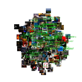
(i) Flickr

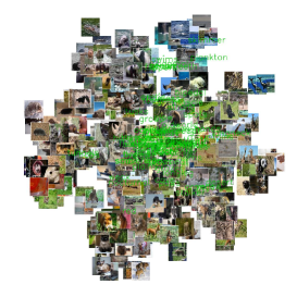
(j) AwA2

Figure 10: Visualization of PMvGE using stochastic neighbor graph.

ROC-AUC scores and variance scores considered in Section 4.2, 4.3 are shown in the following Table 7.

Table 7: ROC-AUC and variance scores are listed; $t$-SNE is applied to obtain $2$-dimensional vectors for $K>2$. Best score is bolded and the second best is underlined.

		ROC-AUC		Variance score
		Flickr	AwA2	Flickr	AwA2
MR-SNE	(unnorm)	0.7134	0.7117	1.706	56.563
	(norm)	0.7038	0.7161	1.388	26.139
	(PMI)	0.6690	0.7109	1.151	27.800
	(weight+unnorm)	0.7000	0.8033	1.556	1.087
	(weight+norm)	0.6902	0.8124	1.475	1.190
	(weight+PMI)	0.6542	0.8134	1.067	1.165
PMvGE + SN graph	$(K=2)$	0.6966	0.8588	1.143	0.042
	$(K=100)$	0.6717	0.8863	1.064	2.670

Overall, PMvGE using SN graph demonstrates good ROC-AUC scores; the score is better than MR-SNE for AwA2, though worse for Flickr dataset. Similarly to most of other baselines, variance score is far from $1$ for AwA2 dataset; MR-SNE with proper weights is yet more stable than the PMvGE using SN graph.

Appendix F CDMCA and Kernel CDMCA

Canonical Correlation Analysis (CCA; Harold,, 1936) is one of the most well-known and widely-accepted methods for multi-view data analysis. However, CCA is designed for considering one-to-one correspondence across domains, meaning that across-domains graph cannot be considered in CCA; Cross-Domain Matching Correlation Analysis (CDMCA; Shimodaira,, 2016) extends CCA so that the across-domains graph is considered. In fact, a special case of (kernel) CDMCA for $2$ domains is obtained by applying (kernel) CCA to preprocessed data vectors; the procedure is shown in the following Section F.1.

For implementation of CCA and kernel CCA, we employ Pyrcca (Bilenko and Gallant,, 2016), that is an open-source Python package for kernel CCA; therein, we specify the regularization parameter by $\lambda=0.01$.

F.1 Preprocessing

Assuming that an across-domains graph $W=(w_{ij})\in\{0,1\}^{n_{1}\times n_{2}}$ is observed. Note that, we here consider only the binary weights $w_{ij}\in\{0,1\}$ representing links in the graph, and within-domain graphs are not considered. Then, we first compute a set of index pairs whose corresponding weights are positive, i.e., $\mathcal{S}:=\{(i,j)\mid 1\leq i\leq n_{1},1\leq j\leq n_{2},w_{ij}=1\}$; by assigning new symbols, the set can also be written as

$$\mathcal{S}=\{(i_{1},j_{1}),(i_{2},j_{2}),\ldots,(i_{m},j_{m})\},$$

where $m\in\mathbb{N}$ is the number of links in the graph. Then, by specifying new data vectors

$$\tilde{x}^{(1)}_{k}=x^{(1)}_{i_{k}},\quad\tilde{x}^{(2)}_{k}=x^{(2)}_{j_{k}},\quad(k=1,2,\ldots,m),$$ (11)

the two data vectors in the pair $(\tilde{x}^{(1)}_{k},\tilde{x}^{(2)}_{k})$ are associated by the link; we have copied the same data vectors several times when they have multiple links. Now, the preproccessed new data vectors $\{\tilde{x}^{(1)}_{k}\}_{k=1}^{m},\{\tilde{x}^{(2)}_{k}\}_{k=1}^{m}$ have one-to-one association with positive weight $w_{i_{k}j_{k}}=1$ as illustrated in Figure 11. Applying CCA to the preprocessed new data vectors (11) is equivalent to a special case of CDMCA for $2$-domains; kernel CDMCA is also similarly defined, by applying kernel CDMCA (Lai and Fyfe,, 2000) to the data vectors (11).

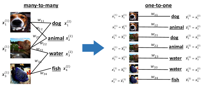
Figure 11: Many to many relations can be converted to one-to-one relations by duplicating some data vectors; applying CCA to the new data vectors yields CDMCA ($D=2$).

References

- Belkin and Niyogi, (2003) Belkin, M. and Niyogi, P. (2003). Laplacian Eigenmaps for Dimensionality Reduction and Data Representation. Neural Computation, 15(6):1373–1396.
- Bilenko and Gallant, (2016) Bilenko, N. Y. and Gallant, J. L. (2016). Pyrcca: Regularized kernel canonical correlation analysis in python and its applications to neuroimaging. Frontiers in Neuroinformatics, 10:49.
- Bradley, (1997) Bradley, A. P. (1997). The use of the area under the ROC curve in the evaluation of machine learning algorithms. Pattern Recognition, 30(7):1145–1159.
- Cayton, (2005) Cayton, L. (2005). Algorithms for manifold learning. Technical report, University of California, San Diego. CS2008-092.
- Chu and Tsai, (2017) Chu, W.-T. and Tsai, Y.-L. (2017). A hybrid recommendation system considering visual information for predicting favorite restaurants. World Wide Web, 20(6):1313–1331.
- Church and Hanks, (1990) Church, K. W. and Hanks, P. (1990). Word association norms, mutual information, and lexicography. Computational Linguistics, 16(1):22–29.
- Davidson et al., (2010) Davidson, J., Liebald, B., Liu, J., Nandy, P., Van Vleet, T., Gargi, U., Gupta, S., He, Y., Lambert, M., Livingston, B., et al. (2010). The YouTube video recommendation system. In Proceedings of the fourth ACM Conference on Recommender Systems, pages 293–296.
- Harold, (1936) Harold, H. (1936). Relations between two sets of variates. Biometrika, 28(3/4):321–377.
- He et al., (2016) He, K., Zhang, X., Ren, S., and Sun, J. (2016). Deep residual learning for image recognition. In Proceedings of the IEEE Conference on Computer Vision and Pattern Recognition, pages 770–778.
- Hong et al., (2014) Hong, C., Yu, J., Tao, D., and Wang, M. (2014). Image-Based Three-Dimensional Human Pose Recovery by Multiview Locality-Sensitive Sparse Retrieval. IEEE Transactions on Industrial Electronics, 62(6):3742–3751.
- Lai and Fyfe, (2000) Lai, P. L. and Fyfe, C. (2000). Kernel and nonlinear canonical correlation analysis. International Journal of Neural Systems, 10(05):365–377.
- Maaten and Hinton, (2008) Maaten, L. v. d. and Hinton, G. (2008). Visualizing data using t-SNE. Journal of Machine Learning Research, 9(Nov):2579–2605.
- Mathew et al., (2016) Mathew, P., Kuriakose, B., and Hegde, V. (2016). Book Recommendation System through content based and collaborative filtering method. In Proceedings of the 2016 International Conference on Data Mining and Advanced Computing, pages 47–52. IEEE.
- Mikolov et al., (2013) Mikolov, T., Sutskever, I., Chen, K., Corrado, G. S., and Dean, J. (2013). Distributed representations of words and phrases and their compositionality. In Advances in Neural Information Processing Systems, pages 3111–3119.
- Mimno and Thompson, (2017) Mimno, D. and Thompson, L. (2017). The strange geometry of skip-gram with negative sampling. In Proceedings of the 2017 Conference on Empirical Methods in Natural Language Processing, pages 2873–2878.
- Okuno et al., (2018) Okuno, A., Hada, T., and Shimodaira, H. (2018). A probabilistic framework for multi-view feature learning with many-to-many associations via neural networks. In Proceedings of the 35th International Conference on Machine Learning, volume 80 of Proceedings of Machine Learning Research, pages 3888–3897. PMLR.
- Pearson, (1901) Pearson, K. (1901). Principal components analysis. The London, Edinburgh, and Dublin Philosophical Magazine and Journal of Science, 6(2):559.
- Pennington et al., (2014) Pennington, J., Socher, R., and Manning, C. D. (2014). Glove: Global vectors for word representation. In Proceedings of the 2014 Conference on Empirical Methods in Natural Language Processing, pages 1532–1543.
- Quadrianto and Lampert, (2011) Quadrianto, N. and Lampert, C. H. (2011). Learning Multi-View Neighborhood Preserving Projections. In Proceedings of the 28th International Conference on Machine Learning, page 425–432.
- Rumelhart et al., (1987) Rumelhart, D. E., Hinton, G. E., and Williams, R. J. (1987). Learning Internal Representations by Error Propagation. In Parallel Distributed Processing: Explorations in the Microstructure of Cognition: Foundations, volume 1, chapter 8, pages 318–362. MIT Press, Cambridge, MA, USA.
- Sharma et al., (2012) Sharma, A., Kumar, A., Daume, H., and Jacobs, D. W. (2012). Generalized Multiview Analysis: A Discriminative Latent Space. In Proceedings of the 2012 IEEE Conference on Computer Vision and Pattern Recognition, pages 2160–2167. IEEE.
- Shimodaira, (2016) Shimodaira, H. (2016). Cross-validation of matching correlation analysis by resampling matching weights. Neural Networks, 75:126–140.
- Sun and Chen, (2007) Sun, T. and Chen, S. (2007). Locality preserving CCA with applications to data visualization and pose estimation. Image and Vision Computing, 25(5):531–543.
- Szegedy et al., (2016) Szegedy, C., Vanhoucke, V., Ioffe, S., Shlens, J., and Wojna, Z. (2016). Rethinking the inception architecture for computer vision. In Proceedings of the 2016 IEEE Conference on Computer Vision and Pattern Recognition, pages 2818–2826. IEEE.
- Talwalkar et al., (2008) Talwalkar, A., Kumar, S., and Rowley, H. (2008). Large-Scale Manifold Learning. In 2008 IEEE Conference on Computer Vision and Pattern Recognition, pages 1–8. IEEE.
- Tang et al., (2015) Tang, J., Qu, M., Wang, M., Zhang, M., Yan, J., and Mei, Q. (2015). LINE: Large-scale Information Network Embedding. In Proceedings of the 24th International Conference on World Wide Web, pages 1067–1077.
- Tenenbaum et al., (2000) Tenenbaum, J. B., De Silva, V., and Langford, J. C. (2000). A global geometric framework for nonlinear dimensionality reduction. Science, 290(5500):2319–2323.
- Thomee et al., (2016) Thomee, B., Shamma, D. A., Friedland, G., Elizalde, B., Ni, K., Poland, D., Borth, D., and Li, L.-J. (2016). YFCC100M: The new data in multimedia research. Communications of the ACM, 59(2):64–73.
- Torgerson, (1952) Torgerson, W. S. (1952). Multidimensional scaling: I. Theory and method. Psychometrika, 17(4):401–419.
- Ulyanov, (2016) Ulyanov, D. (2016). Multicore-TSNE. https://github.com/DmitryUlyanov/Multicore-TSNE.
- van der Maaten, (2014) van der Maaten, L. (2014). Accelerating t-SNE using Tree-Based Algorithms. Journal of Machine Learning Research, 15(93):3221–3245.
- Wang and Zhang, (2013) Wang, F. and Zhang, D. (2013). A New Locality-Preserving Canonical Correlation Analysis Algorithm for Multi-View Dimensionality Reduction. Neural processing letters, 37(2):135–146.
- Xian et al., (2018) Xian, Y., Lampert, C. H., Schiele, B., and Akata, Z. (2018). Zero-Shot Learning-A Comprehensive Evaluation of the Good, the Bad and the Ugly. IEEE Transactions on Pattern Analysis and Machine Intelligence, 41(9):2251–2265.
- Xie et al., (2011) Xie, B., Mu, Y., Tao, D., and Huang, K. (2011). m-SNE: Multiview stochastic neighbor embedding. IEEE Transactions on Systems, Man, and Cybernetics, Part B (Cybernetics), 41(4):1088–1096.
- Zhao et al., (2013) Zhao, X., Evans, N., and Dugelay, J.-L. (2013). Unsupervised multi-view dimensionality reduction with application to audio-visual speaker retrieval. In 2013 IEEE International Workshop on Information Forensics and Security, pages 7–12. IEEE.
Supplementary Material: