Kink dynamics and quantum simulation of supersymmetric lattice Hamiltonians

Abstract

We propose a quantum simulation of a supersymmetric lattice model using atoms trapped in a 1D configuration and interacting through a Rydberg dressed potential. The elementary excitations in the model are kinks or (in a sector with one extra particle) their superpartners - the skinks. The two are connected by supersymmetry and display identical quantum dynamics. We provide an analytical description of the kink/skink quench dynamics and propose a protocol to prepare and detect these excitations in the quantum simulator. We make a detailed analysis, based on numerical simulation, of the Rydberg atom simulator and show that it accurately tracks the dynamics of the supersymmetric model.

Introduction. Models of strongly interacting fermions are key to our understanding of condensed matter systems. At the same time, they are notoriously hard to track, even with sophisticated tools ranging from numerical approaches such as quantum Monte-Carlo Suzuki (1993); Gubernatis et al. (2016); Becca and Sorella (2017) and tensor networks Orús (2014); Montangero et al. (2018) to application of gauge-gravity duality Zaanen et al. (2015). One strategy to make progress is to consider models with special symmetries. A non-standard but intriguing choice is to consider supersymmetry as an explicit symmetry on the lattice Nicolai (1976); Fendley et al. (2003a, b); Fu et al. (2017); Sannomiya et al. (2017); O’Brien and Fendley (2018) or as an emergent symmetry Grover et al. (2014); Huijse et al. (2014); Yu and Yang (2010).

${\cal N}=2$ supersymmetry in a lattice model or a quantum field theory comes with a number of tools, such as the Witten index Witten (1982), which facilitate the analysis. Exploiting these tools unveils remarkable features such as extensive ground state degeneracies, a phenomenon dubbed superfrustration van Eerten (2005); Fendley and Schoutens (2005) which can lead to multicriticality Chepiga et al. (2021).

Despite the supersymmetry, many hard questions remain, such as the nature of the quantum phases in higher spatial dimensions. Here a quantum simulator might provide ingenious insights to these questions. We make a step in this direction and propose such a simulator using arrays of neutral atoms trapped in optical potentials and dressed to their Rydberg state. This is motivated by the high versatility of these platforms Browaeys and Lahaye (2020); Barredo et al. (2016); Endres et al. (2016); Barredo et al. (2018); Wang et al. (2019); Schauß et al. (2015); Labuhn et al. (2016); Bernien et al. (2017); de Léséleuc et al. (2019); Helmrich et al. (2020) and by the fact that an off-resonant dressing Balewski et al. (2014); Jau et al. (2016); Zeiher et al. (2016); Arias et al. (2019) naturally implements the constrained dynamics inherent to the supersymmetric lattice model. Specifically, we consider a so-called M₁ model for spin-less fermions on a 1D chain Fendley et al. (2003a). As a function of a parameter $\lambda$, this model interpolates between a trivial ($\lambda=0$) and a quantum critical ($\lambda=1$) phase, the latter connecting to superconformal field theory Fendley et al. (2003a); Huijse (2011). The value of the Witten index $W=2$ indicates the existence of two supersymmetric vacua and points at kinks connecting these two vacua as elementary excitations. Furthermore, in a sector with one particle added, the excitations correspond to the superpartners of the kinks, which we call the skinks. We propose a protocol for the (s)kink preparation and detection and solve for their dynamics following a quench (we note a recent study of kink-antikink pair dynamics in a spin chain Milsted et al. (2020)). We show that it is identical in both cases and accurately reproduced by the quantum simulator which is a direct consequence and a clear-cut sign of the underlying supersymmetry.

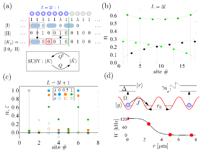
Figure 1: (a) An infinite chain with staggering $11\lambda$ can accommodate two ground states $\ket{{\rm I}},\ket{{\rm II}}$. The lowest energy states for an open chain of length $L=3l+1$ and $l$ particles are kinks $\ket{K_{j}}$. A supercharge $Q$ acting on a kink creates a particle at the kink location. The blue oval represents the triplet. (b) Particle densities in the ground state of an open chain, $L=3l$, $\lambda=1$ with an apparent ${\mathbb{Z}}_{3}$ pattern highlighted by the light green, dark green and black datapoints. (c) Particle (filled symbols) and energy (empty symbols) densities of $\ket{K_{1}}$ for $\lambda=0,0.5,1$ (blue circles, orange squares, green diamonds). (d) Scheme of the proposed realization. Atoms in their electronic ground state $\ket{g}$ tunnel in an optical lattice with spacing $r_{0}$ at rate $J$ subject to dressing to a Rydberg state $\ket{r}$. Lower graph shows the dressed potential $W(r)$ for the $\ket{84{\rm}{\rm S}}$ state of ${}^{6}{\rm Li}$ with $\Omega=2\pi\times 10\,{\rm MHz}$, $\Omega/\Delta=1/10$, $C_{6}=645\,{\rm GHz}\cdot\mu{\rm m}^{6}$.

The M₁ model. An ${\cal N}=2$ supersymmetric lattice Hamiltonian for spinless fermions can be defined as

$$H_{Q}=\{Q,Q^{\dagger}\},$$ (1)

where $Q$ is the nilpotent supercharge, $Q^{2}=0$, and the brackets denote the anti-commutator. The M₁ model Fendley et al. (2003a) (on a bipartite graph) arises when $Q=\sum_{i}Q_{i}$ with $Q_{i}=(-1)^{i}\lambda_{i}c^{\dagger}_{i}P_{\braket{i}}$, where $c_{i}$ are fermionic annihilation operators, $\{c_{i},c_{j}\}=\{c_{i}^{\dagger},c_{j}^{\dagger}\}=0$, $\{c_{i},c^{\dagger}_{j}\}=\delta_{ij}$, and $\lambda_{i}\in{\mathbb{C}}$. The M₁ model constraint, stipulating that fermions are not allowed to occupy nearest neighbour sites $\braket{ij}$, is implemented via the projector $P_{\braket{i}}=\prod_{j\in\braket{ij}}P_{j}$, with $P_{j}=1-n_{j}$, $n_{j}=c_{j}^{\dagger}c_{j}$. The Hamiltonian $H_{Q}$ describes nearest neighbour hoppings and local interactions; it preserves the number of particles, $[H_{Q},\sum_{i}n_{i}]=0$.

We now specialize to 1D and specify real $\vec{\lambda}=\{\lambda_{1},\lambda_{2},\ldots,\lambda_{L}\}$, where $L$ is the length of the chain, $\lambda\geq 0$ and $\lambda_{i}$ repeats every 3 sites in a pattern $1\,1\,\lambda$. For this choice of staggering, the M₁ model is known to be integrable Fendley and Hagendorf (2011). We refer to $\lambda=0$ as extreme staggering.

Supersymmetric groundstates. Let us first consider periodic boundary conditions, $L=3l$, $l\in{\mathbb{N}}$ and $\vec{\lambda}=(1,1,\lambda,\ldots,1,1,\lambda)$. In this case, there are two supersymmetric ground states with $E=0$, each at 1/3 filling. At extreme staggering, they are $\ket{{\rm I}}\equiv\ket{t_{1,2}0_{3}\ldots t_{L-2,L-1}0_{L}}$, $\ket{{\rm II}}\equiv\ket{0_{1}0_{2}1_{3}\ldots 0_{L-2}0_{L-1}1_{L}}$, where $t_{j,j+1}=1/\sqrt{2}(c_{j}^{\dagger}+c_{j+1}^{\dagger})\ket{{\rm vac}}$ is the triplet state and $\ket{\rm vac}$ the fermionic vacuum, see Fig. 1a. For an open chain of length $L=3l$, the degeneracy is lifted and we have a single $E=0$ ground state. Ref. Fendley and Hagendorf (2011) analysed the particle densities $\braket{n_{i}}$ in this groundstate, perturbatively in $1/\lambda$. The same particle densities have been studied at the critical point $\lambda=1$ by invoking conformal field theory which provides closed form expressions for the associated scaling functions Huijse (2011); Sup . The corresponding particle densities constitute a direct experimental probe of the M₁ model as they follow a characteristic ${\mathbb{Z}}_{3}$ pattern indicated by the grey lines in Fig. 1b together with the data points (diamonds) for $l=6$ Sup .

Kinks at extreme staggering. For an open chain of $L=3l+1$ there are no supersymmetric groundstates. Instead, at extreme staggering the lowest energy states with $l$ particles interpolate between the ground state configurations $\ket{{\rm I}}$ and $\ket{{\rm II}}$, with an empty site at position $i=3j-2$, with $j=1,\ldots,l+1$. We write these bare kink states as $\ket{K_{j}}=\ket{{\rm I}_{[1,i-1]}0_{i}{\rm II}_{[i+1,L]}}$, where ${\rm I}_{[a,b]}$, ${\rm II}_{[a,b]}$ denote the part of the ground state configuration located between sites $a$ and $b$. They all have energy $E=1$. The labels $j=1\;(j=l+1)$ correspond to the leftmost (rightmost) kink, see Fig. 1a. Acting with the supercharge on the kink increases the number of particles by one creating the kink’s superpartner, the skink, $\ket{\bar{K}_{j}}\equiv Q\ket{K_{j}}=\ket{{\rm I}_{[1,i-1]}1_{i}{\rm II}_{[i+1,L]}}$. Consequently, $Q^{\dagger}\ket{\bar{K}_{j}}=\ket{K_{j}}$ such that $\ket{K_{j}}$ and $\ket{\bar{K}_{j}}$ form doublets under supersymmetry, see Fig. 1a Fokkema and Schoutens (2017). To characterize the kinks, we introduce a local energy density $h_{i}=\frac{1}{2}\left(\{Q,Q^{\dagger}_{i}\}+\{Q^{\dagger},Q_{i}\}\right)$ such that $H_{Q}=\sum_{i=1}^{L}h_{i}$.

Fig. 1c shows the particle density $n=\braket{n_{i}}$ and energy density $\varepsilon=\braket{h_{i}}$ for the leftmost kink $\ket{K_{1}}$ for $\lambda=0$ (blue data). The kink is clearly located at the left end of the chain with a corresponding peak in the energy density.

Kinks at general $\lambda$. We claim that the notion of 1-kink (and multi-kink) states is well defined also away from extreme staggering, when $0<\lambda\leq 1$. To illustrate this, we present in the inset of Fig. 2a the spectrum of the system for $l=4$. The energies become degenerate for $\lambda=0$ taking odd positive values corresponding to the 1-kink, 3-kink, etc. states. The unavoided level crossings, characteristic for integrability, allow us to unambiguously characterize states as multi-kink states for all $\lambda$.

Fig. 2a shows the low-lying part of the spectrum, which includes a band of $l+1$ 1-kink eigenstates $\ket{v_{k}}$ of energy $E_{k}$. We define a localized kink as Minář and Schoutens

$$\ket{K_{j}}=\sqrt{\frac{2}{l+2}}\sum_{k=1}^{l+1}\sin(\tilde{k}j)\ket{v_{k}},$$ (2)

where $\tilde{k}=\pi k/(l+2)$.

In Fig. 1c the orange and green data points show the particle and energy densities in the state $\ket{K_{1}}$ obtained numerically using Eq. (2) for $\lambda=0.5,1$. We see that, even for $\lambda=1$, the kink is well defined with most of its energy localized at the kink position.

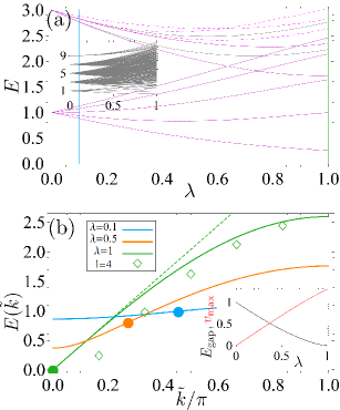
Figure 2: (a) Spectrum (inset) and nine lowest eigenenergies for $l=4$ in $l$ (grey) and $l+1$ (dashed magenta) particle-number sector of $H_{Q}$. (b) The dispersion Eq. (4) for $\lambda=0.1,0.5,1$ (blue, orange, green). The filled circles correspond to the fastest mode $\tilde{k}$ with $v_{\rm max}$. The green diamonds denote the exact eigenenergies for $l=4$ and $\lambda=1$. The green dashed line is an eye-guide depicting the linear dispersion at the origin. The inset shows the gap, i.e. the lowest energy, (black) and $v_{\rm max}$ (red) vs. $\lambda$.

Figure 3: (a) Time evolution of $|o(t)|^{2}$, Eq. (3), (solid lines) and $\delta n$ (dashed lines) for a quench from the exact (blue) and reduced fidelity (red) kink state $\ket{K_{1}}$ for $l=4$. The grey line corresponds to $|o(t)|^{2}$ evaluated with Eq. (4) for the eigenenergies. (b) Numerical evaluation (grey, Eq. (3)) and saddle point approximation (green dashed, red, Eq. (5)) of the overlap $|o(t)|^{2}$ for $l=101$. The green (red) lines correspond to considering the first two (only the second) saddle points. The inset shows the onset of oscillations around $tv_{F}/l=3$. (c) Quench dynamics for 10-site chain ($l=3$), with initial states $\ket{K_{1}^{\prime}}$ (blue) and $\ket{\bar{K}_{1}^{\prime}}$ (magenta). Solid lines show dynamics under the full Hamiltonian $H_{\rm Ry}$, while the grey curve is for a truncation of $H_{\rm Ry}$, neglecting interactions beyond next-nearest neighbours. Dashed lines show dynamics under $H_{Q}$. The red line shows the average population in the Rydberg state $\overline{n^{r}}=1/l\sum_{i}n^{r}_{i}$, while the green line tracks the nearest-neighbour occupation of ground state atoms, $\overline{n_{i}n_{i+1}}=1/l\sum_{i^{\prime}}n_{i^{\prime}}n_{i^{\prime}+1}$. Parameters as in Fig. 1d.

Kink dynamics. We now proceed with the evaluation of the kink dynamics. We start from the leftmost kink $\ket{K_{1}}$ and consider overlap at time $t$ with the rightmost kink, $o(t)\equiv\braket{K_{l+1}}{K_{1}(t)}$, where $\ket{K_{1}(t)}={\rm e}^{-iH_{Q}t}\ket{K_{1}}$. It follows from Eq. (2) that

$$o(t)=\frac{2}{l+2}\sum_{k=1}^{l+1}\sin\left(\tilde{k}\right)\sin\left(\tilde{k}(l+1)\right){\rm e}^{-iE_{k}t}.$$ (3)

For simplicity, from now on we focus on the critical case $\lambda=1$. In Fig. 3a we show $|o(t)|^{2}$ for $l=4$ (solid blue line). At criticality, the fastest mode propagates with the Fermi velocity $v_{F}$, see the discussion after Eq. (4). This results in the onset of the overlap at $tv_{F}/l\approx 1$, with the maximum achieved for a later time, $tv_{F}/l\approx 1.75$.

Kink detection. To make a connection with experimentally observable quantities, we construct an observable $\delta n$ which detects the presence of a kink at the right end of the system, by requiring that $\braket{K_{i}}{\delta n}{K_{j}}\approx\delta_{i,l+1}\delta_{j,l+1}$. Taking $\delta n=\alpha(\lambda,l)\left[1-\beta(\lambda,l)\left(n_{L-1}+n_{L+1}\right)\right]$ we find $\alpha(0,l)=1$, $\beta(0,l)=1$ for any $l$ and $\alpha(1,l)\approx 1.08$, $\beta(1,l)\approx 1.09$ for $l=3,4$ Sup . The numerically obtained result for $\delta n(t)$ is shown as a blue dashed line in Fig. 3a and corresponds to a good accuracy to $|o|^{2}$.

Kink preparation. An important question is how the spatially localized kink $\ket{K_{1}}$ can be prepared in practice. To this end we note that the kink site and its nearest neighbours remain approximately empty for all $\lambda$, cf. Fig. 1c. We thus consider an adiabatic preparation of a ground state $\ket{K_{1}^{\prime}}$ of the final Hamiltonian $H_{f}=H_{Q}+\mu(n_{1}+n_{2})$, where $\mu\rightarrow\infty$ ensures the kink condition on the first two sites. The initial Hamiltonian is chosen such that its ground state is a kink at extreme staggering $\lambda=0$ (and similarly for skinks below), cf. Sup . For $l=4$ we find the fidelities $F\in[0.95,1]$, where $F=|\braket{K_{1}^{\prime}}{K_{1}}|$, with the highest (lowest) value at extreme staggering (criticality). In Fig. 3a we show the numerically evaluated overlap $|o^{\prime}|^{2}=|\braket{K_{l+1}}{K_{1}^{\prime}(t)}|^{2}$ and the corresponding observable $\delta n^{\prime}$ as solid (dashed) red lines. We find that despite the limited fidelity of the initial state, $|o^{\prime}|^{2}$ and $\delta n^{\prime}$ agree well with $|o|^{2}$ and $\delta n$.

Skinks. Supersymmetry guarantees that the 1-skink energies (the lower dashed magenta lines in Fig. 2a) in the sector with $l+1$ particles are identical to the 1-kink energies $E_{k}$. As a consequence, the quench dynamics for the skinks is again given by Eq. (3). For the detection of $\ket{\bar{K}_{l+1}}$ we propose $\delta\bar{n}=-\bar{\alpha}(\lambda,l)\left[1-\bar{\beta}(\lambda,l)\left(n_{L-2}+n_{L-1}+n_{L+1}\right)\right]$ with $\bar{\alpha}(0,l)=2$, $\bar{\beta}(0,l)=1$ and $\bar{\alpha}(1,l)\approx 1.46$, $\bar{\beta}(1,l)\approx 0.98$ for $l=3,4$. For the preparation we find that the ground state $\ket{\bar{K}_{1}^{\prime}}$ of $H_{f}=H_{Q}+3(-n_{1}+n_{2}-0.5n_{3})$ corresponds well to $\ket{\bar{K}_{1}}$ Sup . The $l=4$ fidelities are $\bar{F}\in[0.93,1]$ with $\bar{F}=|\braket{\bar{K}_{1}^{\prime}}{\bar{K}_{1}}|$.

Kink/skink dynamics at large $l$. Surprisingly, the kink arrival amplitude Eq. (3) is analytically tractable, for general $\lambda$, in the large-$l$ limit. A key element for this is the continuum limit $E(\tilde{k})$ of the kink dispersion relation. Exploiting a relation between the M₁ model and the XYZ spin-1/2 chain Fendley and Hagendorf (2010), we have found Minář and Schoutens

$$E(\tilde{k})=\frac{\left(3\lambda+s\right)^{3/2}\sqrt{1-\left(1-\frac{\left(-3\lambda+s\right)^{3}\left(\lambda+s\right)}{\left(-\lambda+s\right)\left(3\lambda+s\right)^{3}}\right)\cos^{2}\left(\frac{\tilde{k}}{2}\right)}}{2\sqrt{2}\sqrt{\lambda+s}},$$ (4)

where $s=\sqrt{8+\lambda^{2}}$. In Fig. 2b we show the dispersion for $\lambda=0.1,0.5,1$. We denote by $v_{\rm max}(\lambda)$ the maximum value of the group velocity $v(\tilde{k})=\partial_{\tilde{k}}E(\tilde{k})$. At criticality, $v_{\rm max}(\lambda=1)=v_{F}=3\sqrt{3}/4$, with $v_{F}$ the Fermi velocity. This gives real space velocity (since kinks hop three sites at a time) $3v_{F}=9\sqrt{3}/4$, in agreement with Huijse (2011).

In Fig.  3a the grey line shows the overlap Eq. (3) evaluated with the energies $E(\tilde{k})$ instead of $E_{k}$ (blue line). The difference is a consequence of finite $l$, cf. the green diamonds vs. green solid line in Fig. 2b.

Using the dispersion $E(\tilde{k})$ we can evaluate the large-$l$ limit of Eq. (3) in a saddle point approximation Sup , giving

$$o(t) \approx \frac{2}{l+2}\sum_{s=1}^{\infty}\theta\left(\frac{v_{\rm max}t}{l+2}-(2s-1)\right)\sin\left(\tilde{k}_{s}\right)^{2}$$ (5)

$${\rm e}^{i\left[(2s-1)\pi k_{s}+E(\tilde{k}_{s})t\right]+i\frac{5\pi}{4}}\sqrt{\frac{2\pi}{-E^{\prime\prime}(\tilde{k}_{s})t}},$$

where $\theta$ is the Heaviside step function, $k_{s}=\left.E^{\prime}\right.^{-1}\left((2s-1)\pi/t\right)$, $E^{\prime}=\partial_{k}E(\tilde{k})$, $E^{\prime\prime}=\partial^{2}_{k}E(\tilde{k})$ and $s$ labels the saddle point corresponding to the arrival times $t=(2s-1)(l+2)/v_{\rm max}\approx(2s-1)l/v_{\rm max}$, $s\in\mathbb{N}$, of the kink front (maximum velocity mode). At criticality, where $E(\tilde{k})=2v_{F}\sin(\tilde{k}/2)$, the saddle point expression takes a simple closed form Sup .

In Fig. 3b we show an example of the dynamics for $l=101$ evaluated using Eq. (3) (grey line) together with the prediction of Eq. (5) (green dashed line). We see a close to perfect agreement, with the inset showing the details around $tv_{F}/l=3$, where the second saddle point, $s=2$, starts to generate the characteristic modulation of the overlap due to the interference of the kink front propagating at $v_{F}$ incident on the right edge (after it has undergone one round trip) and the kink tail. We note the frequency chirp of the modulation due to the non-trivial time dependence of $\tilde{k}_{s}$. Here we do not show the observable $\delta n(t)$ as for large $l$ the Hamiltonian cannot be diagonalized exactly.

Experimental implementation. We now discuss how $H_{Q}$ can be engineered using Rydberg dressed atoms Henkel et al. (2010); Pupillo et al. (2010). We consider effectively two-level atoms with the ground and Rydberg states $\ket{g}$, $\ket{r}$, where the ground state atoms experience an optical lattice potential and the atoms in a Rydberg state a repulsive Van der Waals interaction described by

$$H_{\rm Ry} = -J\sum_{i=1}^{L-1}\left(c^{\dagger}_{i+1}c_{i}+c^{\dagger}_{i}c_{i+1}\right)+\sum_{i=1}^{L}\mu_{i}n_{i}$$ (6)

$$+\sum_{i=1}^{L}\Omega\sigma^{x}_{i}+\Delta n^{r}_{i}+\sum_{i>j=1}^{L-1}V_{ij}n^{r}_{i}n^{r}_{j}.$$

Here, $J>0$ is the hopping amplitude, $\sigma^{x}=\ket{r}\bra{g}+\ket{g}\bra{r}$, $n^{r}=\ket{r}\bra{r}$ and $V_{ij}=C_{6}/(r_{0}|i-j|)^{6}$ with $C_{6}$ the Van der Waals coefficient and $r_{0}$ the lattice spacing. We consider a regime of large detuning $\Omega/\Delta\ll 1$, where the ground state atoms interact, up to order $\Omega^{4}$, through an effective flat-top potential $W(r=r_{0}|i-j|)=2\Omega^{4}V_{ij}/[\Delta^{3}(V_{ij}+2\Delta)]$, cf. Fig. 1d. To obtain the supersymmetric $H_{Q}$, the interaction and chemical potentials $W$, $\mu$ and the hopping $J$ need to be tuned as follows.

For simplicity, we refer the discussion of general $\lambda$ to Sup and focus on $\lambda=1$. In this case the chemical potential terms in $H_{Q}$ become site-independent up to the boundary terms originating from $P_{1}P_{3}$ and $P_{L-2}P_{L}$, which can be accounted for by setting $\mu_{1}=\mu_{L}=J$.

Next, the M₁ model Hamiltonian forbids nearest neighbour occupation while the potential terms are of the form $P_{i-1}P_{i+1}$, with no interactions beyond lattice distance 2. For this to be captured by the flat-top potential we need $W(r_{0})/W(2r_{0})\gg 1$ and $W(2r_{0})/W(3r_{0})\gg 1$ with the maximum achieved in the limit $r_{0}\rightarrow\infty$. However, to counteract experimental imperfections Sup , one should reduce the duration of the simulation by maximizing the relevant energy scale, here $W(2r_{0})$, which happens for $r_{0}\rightarrow 0$ and one has to set $J=W(2r_{0})$. This corresponds to the optimal approximation of $H_{Q}$ using single dressing. Importantly, we show in Sup that $H_{Q}$ can be reached in principle with arbitrary number of dressings with already a tenfold increase in $W(r_{0})/W(2r_{0})$ and $W(3r_{0})/W(2r_{0})$ for a double dressing with realistic parameters.

As a specific example, we consider the fermionic ${}^{6}{\rm Li}$ dressed with the $\ket{84{\rm S}}$ state with $C_{6}=645\,{\rm GHz}\cdot\mu{\rm m}^{6}$ Šibalić et al. (2017, ) and lattice spacing $r_{0}=2.5\,\mu{\rm m}$. The resulting dressed potential is shown in Fig. 1d. We get $W(2r_{0})=J\approx 4\,{\rm kHz}$, which for the optical lattice laser wavelength $\lambda=2r_{0}=5\,\mu{\rm m}$ corresponds to lattice depth $\approx 5.5E_{r}$, $E_{r}$ being the recoil energy Arzamasovs and Liu (2017) .

Fig. 3c shows the quantum simulation of $H_{Q}$, where we compare the dynamics generated by the Rydberg Hamiltonian (6) with that of $H_{Q}$ quenching from $\ket{K_{1}^{\prime}}$ and $\ket{\bar{K}_{1}^{\prime}}$, see caption for details. We draw two main conclusions. First, the quantum simulator accurately tracks the dynamics set by the model hamiltonian $H_{Q}$ and, second, the dynamics in the $l$-particle sector (blue lines) is highly similar to that in the $l+1$ particle sector (magenta lines). The latter observation is direct evidence of the supersymmetry of $H_{Q}$.

Outlook. We have proposed a realization of a supersymmetric lattice Hamiltonian $H_{Q}$ based on atoms interacting through a Rydberg dressed potential Weimer et al. (2012a, b). Our results constitute a stepping stone to quantum simulations of supersymmetric lattice models in higher dimensions Fendley and Schoutens (2005); Huijse et al. (2008, 2012); Galanakis et al. (2012); Surace et al. (2020), which can require $n$-body, rather than 2-body, interactions. In this context, it would be interesting to consider a scheme relying on coupling the Rydberg atoms with phonons Gambetta et al. (2020) or to use cold molecules with permanent or electric-field induced dipole moments, avoiding the need for off-resonant dressing Büchler et al. (2007); Carr et al. (2009); Baranov et al. (2012); Balakrishnan (2016). Another interesting avenue is to exploit the mapping of the supersymmetric lattice Hamiltonians to spins Fendley et al. (2003b); Fendley and Hagendorf (2010); Chepiga et al. (2021); Minář and Schoutens which would allow for simulations with platforms such as superconducting devices with $n$-body interactions Pedersen et al. (2019); Roy et al. (2020).

Acknowledgments. We are very grateful to P. Fendley, I. Lesanovsky, Y. Miao, E. Ilievski, N. Chepiga, F. Schreck, K. van Druten, R. Spreeuw, R. Gerritsma, T. Lahaye, B. Pasquiou, V. Barbé and A. Urech for stimulating discussions. This work is part of the Delta ITP consortium, a program of the Netherlands Organisation for Scientific Research (NWO) that is funded by the Dutch Ministry of Education, Culture and Science (OCW).

I Ground state particle densities

In this section we recall the expressions for single particle densities for the M₁ model at criticality, on an open chain of length $L=3l$. We used these expressions to produce the grey lines in Fig. 1b. Exploiting the tools of conformal field theory, the model can be mapped to a free boson and the particle densities can be expressed in terms of the correlators of the bosonic vertex operators with a characteristic ${\mathbb{Z}}_{3}$ pattern Huijse (2011). Specifically, they read

$$n_{3j-2} =\frac{1}{3}-\frac{2A}{3}\frac{s(x)}{{\mathfrak{s}}(x)}$$ (S1a)

$$n_{3j-1} =\frac{1}{3}+\frac{2A}{3}\frac{c(x-L^{\prime}/2)}{{\mathfrak{s}}(x)}$$ (S1b)

$$n_{3j} =\frac{1}{3}+\frac{2A}{3}\frac{s(x-L^{\prime})}{{\mathfrak{s}}(x)},$$ (S1c)

where $x\in[2,L]$, $L^{\prime}=L+3$ and

$$s(x) =\left(\frac{\pi}{2L^{\prime}}\right)^{\frac{1}{3}}\sin\left(\frac{\pi x}{3L^{\prime}}\right)$$ (S2a)

$$c(x) =\left(\frac{\pi}{2L^{\prime}}\right)^{\frac{1}{3}}\cos\left(\frac{\pi x}{3L^{\prime}}\right)$$ (S2b)

$${\mathfrak{s}}(x) =\sin\left(\frac{\pi x}{L^{\prime}}\right)^{\frac{1}{3}}.$$ (S2c)

Here, the parameter $A$ has been determined numerically as $A=0.77$ Huijse (2011). We note that analogous results hold for $L=3l-1$ Huijse (2011).

II (S)kink profiles and design of the observables

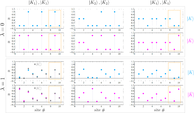
Figure S1: Single site particle densities of kinks (blue data points) and skinks (magenta data points) for $l=3$ at extreme staggering $\lambda=0$ (first two rows) and at criticality $\lambda=1$ (third and fourth row) for the leftmost (s)inks $\ket{K_{1}},\ket{\bar{K}_{1}}$ (first column), $\ket{K_{2}},\ket{\bar{K}_{2}}$ (second column) and the rightmost (s)kinks $\ket{K_{4}},\ket{\bar{K}_{4}}$ (third column). The gray data points for $\lambda=1$ indicate the densities evaluated with $\ket{K_{1}^{\prime}}$ and $\ket{\bar{K}_{1}^{\prime}}$ for kinks and skinks respectively, see text for details.

To motivate the choice of observables, we will first examine the kink and skink profiles. Fig. S1 shows the single site particle densities of kinks (blue data points) and skinks (magenta data points) for $l=3$ at extreme staggering, $\lambda=0$, (first two rows) and at criticality, $\lambda=1$, (third and fourth row) for the leftmost (s)inks $\ket{K_{1}},\ket{\bar{K}_{1}}$ (first column), $\ket{K_{2}},\ket{\bar{K}_{2}}$ (second column) and the rightmost (s)kinks $\ket{K_{4}},\ket{\bar{K}_{4}}$ (third column). We wish to design observables which capture the properties of the overlaps $o(t)=\braket{K_{l+1}}{K_{1}(t)}=\braket{\bar{K}_{l+1}}{\bar{K}_{1}(t)}=\bar{o}(t)$ signalling the arrival of the leftmost kink to the right edge. Motivated by the (s)kink profiles, we in particular examine the situation in the last unit cell corresponding to the last three sites of the chain and to staggering $1\lambda 1$ indicated by the orange boxes in Fig. S1. For the observable we consider a function of the particle densities on these three sites, $\delta n=\delta n(n_{L-2},n_{L-1},n_{L})$, and require that $\braket{K_{i}}{\delta n}{K_{j}}\approx\delta_{i,l+1}\delta_{j,l+1}$. We find that these conditions are satisfied by imposing

$$\braket{K_{1}}{\delta n}{K_{1}} =0$$ (S3a)

$$\braket{K_{l+1}}{\delta n}{K_{l+1}} =1$$ (S3b)

and similarly for the skinks.

At extreme staggering, the occupation of the last unit cell is 1 and 1/2 for $\ket{K_{1}}$ and $\ket{K_{l+1}}$ (1 and 3/2 for $\ket{\bar{K}_{1}}$ and $\ket{\bar{K}_{l+1}}$). We also note, that for kinks the total particle number at the last two sites is different for $\ket{K_{1}}$ and $\ket{K_{l+1}}$, but the same for the skinks. In contrast to the extreme staggering, at criticality (and generally for $\lambda>0$) the total particle number in the last unit cell varies and is not equal to integer or half-integer values. This motivates us to introduce the following observables

$$\delta n =\alpha(\lambda,l)\left[1-\beta(\lambda,l)\left(n_{L-1}+n_{L+1}\right)\right]$$ (S4a)

$$\delta n_{3} =\alpha_{3}(\lambda,l)\left[1-\beta_{3}(\lambda,l)\left(n_{L-2}+n_{L-1}+n_{L+1}\right)\right]$$ (S4b)

$$\delta\bar{n} =-\bar{\alpha}(\lambda,l)\left[1-\bar{\beta}(\lambda,l)\left(n_{L-2}+n_{L-1}+n_{L+1}\right)\right],$$ (S4c)

where the coefficients $\alpha,\beta$ in general depend on $\lambda$ and the chain length $L=3l+1$, where the latter is to be expected, similarly to the presence of such scaling in the particle densities (S1) of the ground state of chain of length $L=3l$. At extreme staggering, the value of the coefficients can be read-off directly from Fig. S1 and we obtain

$$\lambda=0:$$

$$(\alpha,\beta) =(1,1)$$ (S5a)

$$(\alpha_{3},\beta_{3}) =(2,1)$$ (S5b)

$$(\bar{\alpha},\bar{\beta}) =(2,1)$$ (S5c)

which are independent of $l$. For $\lambda=1$, the values are obtained from the defining property (S3) and their scaling with $l$ is shown in Fig. S2a-f (up to $l=6$). We use these values in the analysis of the critical dynamics.

To examine the observables, in Fig. S2g we show the (square of the) overlap (gray) together with $\delta n,\delta n_{3}$ (solid and dashed blue) and $\delta\bar{n}$ (magenta) for a quench from $\ket{K_{1}}$ and $\ket{\bar{K}_{1}}$ respectively with the dynamics generated by the supersymmetric Hamiltonian $H_{Q}$, Eq. (1). We see that the proposed observables nicely capture the overlap function $|o|^{2}$.

Figure S2: Scaling of the coefficients (a,d) $\alpha,\beta$, (b,e) $\alpha_{3},\beta_{3}$ and (c,f) $\bar{\alpha},\bar{\beta}$ parametrizing the observables (S4) with $l$ at criticality, $\lambda=1$. (g) Time evolution of the observables (S4) for $l=3$ following a quench from $\ket{K_{1}}$ (blue lines) and $\ket{\bar{K}_{1}}$ (magenta line) together with the square of the overlap $|o|^{2}=|\braket{K_{l+1}}{K_{1}(t)}|^{2}=|\braket{\bar{K}_{l+1}}{\bar{K}_{1}(t)}|^{2}$ (gray line).

III State preparation

In this section we study state preparation by means of adiabatic following for the two scenarios considered in the main text, an open chain of length $L=3l$ and staggering $1\lambda 1...1\lambda 1$ (scenario 1) and an open chain of length $L=3l+1$ and staggering $11\lambda\ldots 1\lambda 1$ (scenario 2). Motivated by the relative simplicity of the experimental implementation, we focus on the critical case $\lambda=1$. We comment on the (un)suitability of the adiabatic protocol for critical systems at the end of the section.

We consider a preparation of a ground state of a final Hamiltonian $H_{f}$ by adiabatic following from $H_{i}$, such that the time-dependent Hamiltonian can be expressed as

$$H(t)=(1-\mathcal{F}(t))H_{i}+\mathcal{F}(t)H_{f}.$$ (S6)

We consider three distinct cases for $H_{f}$. (i) $H_{f}=H_{Q}$ in (scenario 1), (ii) $H_{f}=H_{Q}+\mu(n_{1}+n_{2})$ with $\mu\rightarrow\infty$ for kink and (iii) $H_{f}=H_{Q}+\bar{\mu}(-n_{1}+n_{2}-\bar{\nu}n_{3})$ with $\bar{\mu},\bar{\nu}\approx 3,1/2$ for skink preparation in (scenario 2). $H_{f}$ in (ii) is chosen to ensure no occupation of the first two sites in preparation of the leftmost kink $\ket{K_{1}}$, a condition well satisfied even at criticality. This is apparent from Fig. S1 ($\lambda=1,\ket{K_{1}}$ pane, blue data points) where we plot the densities corresponding to the ground state $\ket{K^{\prime}_{1}}$ of $H_{f}$ as gray data points. For skinks, enforcing a particle at first site and zero particle on the second yields a density on the third site which is too small as compared with the ideal skink $\ket{\bar{K}_{1}}$. To rectify that, we introduce the $H_{f}$ described in (iii) and optimize the skink fidelity by tuning $\bar{\mu},\bar{\nu}$ with optimal values indicated above. The corresponding densities are shown as gray data points in Fig. S1 ($\lambda=1$, $\ket{\bar{K}_{1}}$ pane).

The function ${\cal F}(t)$ in Eq. (S6) has to be chosen such that it satisfies the adiabatic theorem Messiah (1999); Teufel (2003); Albash and Lidar (2018). In particular, ${\mathcal{F}}(0)=0$, ${\mathcal{F}}(T)=1$, and it is at least twice differentiable. Here $T$ is the duration of the adiabatic sweep. In order to provide a specific example, we consider

$${\mathcal{F}}(t)=\frac{1}{2}\left[1-\cos\left(\pi\frac{t}{T}\right)\right].$$ (S7)

While we focus on a critical system, as we are concerned with experiments with a finite number of atoms, the system will remain gapped (we exploit the rigorous results for the finite size scaling of the gap in Sec. V.5). To this end we consider an approximate but qualitatively sufficient picture that the time duration of the adiabatic sweep $T$ should be much larger than the inverse of the spectral gap $1/\Delta_{sg}$ (see e.g. Messiah (1999); Teufel (2003); Albash and Lidar (2018); Avron and Elgart (1998); Rigolin and Ortiz (2012) for discussion of adiabaticity conditions). We define the spectral gap as the energy difference between the lowest and the first excited state of the Hamiltonian .

Note on the initial Hamiltonian. In order to ensure that no level-crossing occurs as the Hamiltonian is swept from $H_{i}$ to $H_{f}$, some care has to be taken in the choice of $H_{i}$. One possibility is to choose $H_{i}$ such that its ground state is the lowest energy state of $H_{Q}$ at extreme staggering. For the specific lengths and staggerings considered, the $\lambda=0$ states are particularly simple as they are given by product states of the form (see Table 1 for a summary of low energy spectral properties of the M₁ model at extreme staggering)

$$(i) \;L=3l,\;1\lambda 1\ldots\;\rightarrow\;\ket{\psi_{i}}=\ket{010010...}$$ (S8a)

$$(ii) \;L=3l+1,\;11\lambda\ldots\;\rightarrow\;\ket{\psi_{i}}=\ket{001001...}$$ (S8b)

$$(iii) \;L=3l+1,\;11\lambda\ldots\;\rightarrow\;\ket{\psi_{i}}=\ket{101001...}$$ (S8c)

We thus take the initial Hamiltonian, which enforces the $l$ particles to be trapped at sites $s=\{2,5,...\}$, $s=\{3,6,...\}$ for cases (i), (ii) and $l+1$ particles at sites $s=\{1,3,6,...\}$ for (iii), to be of the form

$$H_{i}=-\sum_{i}(\alpha i+\mu_{0})n_{i}-\mu\sum_{i\in s}n_{i}.$$ (S9)

The first summand is meant to lift remaining degeneracies and in principle more complicated functions of the position $i$ can be considered. In practice, as we are mainly concerned with preserving the gap between the lowest energy and the first excited state, the details of this function are not essential as far as $\mu\gg\mu_{0},\alpha i$ for all $i$, which is used in the following. The state is prepared as

$$\ket{\psi(t)}={\cal T}{\rm e}^{-i\int_{0}^{t}{\rm d}t^{\prime}\,H(t^{\prime})}\ket{\psi_{i}},$$ (S10)

where $H(t)$ is given by (S6), $\cal{T}$ is the usual time ordering operator and $\ket{\psi_{i}}$ are given by (S8) . Press et al. (2007) We further denote the prepared state at the end of the adiabatic evolution as $\ket{\psi_{\rm prep}}\equiv\ket{\psi(T)}$. We then quantify the fidelity of the prepared state as (i) $F=|\braket{\psi_{\rm prep}}{\psi_{0}}|$, where $\ket{\psi_{0}}$ is the ground state of $H_{Q}$ and (ii) $F_{j}=|\braket{\psi_{\rm prep}}{K_{j}}|$, (iii) $\bar{F}_{j}=|\braket{\psi_{\rm prep}}{\bar{K}_{j}}|$. The results for (i) and (ii) are shown in Fig. S3, see the caption for details (the results of (iii) not shown are similar to (ii)). In summary, the fidelity of preparation $F>0.92$ ($F>0.95$ for the boundary kinks $\ket{K_{1}},\ket{K_{l+1}}$ and $\bar{F}>0.91$ for the boundary skinks $\ket{\bar{K}_{1}},\ket{\bar{K}_{l+1}}$) for system sizes we analyzed numerically, i.e. $l\leq 6$.

Optimization. Few remarks are in order with respect to the adiabatic procedure considered. A first technical one is that one can optimize the sweep function (S7) which adapts the rate of change to the instantaneous gap $\Delta_{sg}(t)$ evolving at a slower rate for smaller gaps, which has the potential to significantly reduce the time required to achieve a desired fidelity for a given system size Albash and Lidar (2018). This is desirable as the final (and minimal) gap $\Delta_{sg}(t=T)$ is decreasing with system size, so that using the same ${\mathcal{F}}(t)$ for different system sizes will result in larger times in order to achieve the same target fidelity as is illustrated in Fig. S3. The other remark is qualitative and is about the inadequacy of adiabatic protocols for preparing critical states with a vanishing gap in the thermodynamic limit, requiring an infinitely slow sweep akin to the Kibble-Zurek mechanism. While we consider the adiabatic preparation protocol even in this case, we note that other schemes using spatiotemporal quenches have been proposed recently Agarwal et al. (2018). Whether such a scheme can be implemented in our setup goes beyond the scope of the present work and we leave it for future investigations.

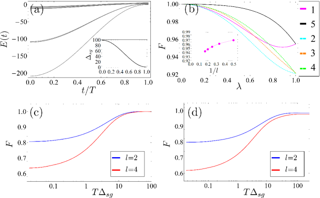
Figure S3: Adiabatic state preparation. (a) Example of the spectrum of the Hamiltonian (S6) for case (i), i.e. $L=3l$ with $l=2$, as a function of time. The inset shows the spectral gap. (b) Fidelity $|\braket{K_{j}^{\prime}}{K_{j}}|$ of the kink states as a function of $\lambda$ for case (ii), $L=3l+1$ with $l=4$. The solid (dashed) lines are for the boundary, i.e. rightmost and leftmost, (bulk) kinks respectively. Here, $\ket{K_{j}^{\prime}}$ are the lowest energy states of the Hamiltonian $H+\mu\sum_{i\in j-{\rm th\;kink}}n_{i}$, where the $\mu$-term enforces no occupation (for $\mu\rightarrow\infty$) on the sites of $j$-th kink, $i=(3(j-1),3(j-1)+1,3(j-1)+2)$ for $1<j<l+1$ and $i=1,2$ ($i=L-1,L$) for the leftmost (rightmost) kink $\ket{K_{1}}$ ($\ket{K_{l+1}}$), see also the main text. The inset shows the finite size scaling of the fidelity of the leftmost kink at criticality for $l=2,3,4,5,6$. (c) Fidelity of the preparation of the ground state as a function of the adiabatic sweep length $T$ for $l=2,4$ (blue, red), i.e. case (i), $L=3l$, $\lambda=1$. (d) Fidelity of the preparation of the leftmost kink $\ket{K_{1}}$ as a function of the adiabatic sweep length $T$ for $l=2,4$ (blue, red), i.e. case (ii), $L=3l+1$, $\lambda=1$. In (c) and (d) the horizontal axes are in terms of $T\Delta_{sg}$, where $\Delta_{sg}=\Delta_{sg}(T)$.

	$11\lambda$ …	$1\lambda 1\ldots$	$\lambda 11\ldots$
$3l-1$	1,0,2	1,0,1	1,0,1
$3l$	1,0,1	1,0,2	1,0,1
$3l+1$	$l+1$,1,2	$l+1$, 1,2	1,0,1

Table 1: Summary of the low energy properties of the M₁ model at extreme staggering $\lambda=0$. The three possible staggerings and system sizes are listed in the top row/left column respectively. The three numbers are $({\rm deg}_{\rm lowest},E_{\rm lowest},\Delta_{sg})=$(degeneracy of the lowest energy manifold, energy of the lowest energy states, spectral gap between the lowest and first excited state).

IV Saddle point approximation

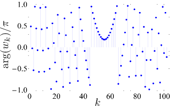
Figure S4: Argument of the summands $w_{k}$ in (S11) for $l=101,t=120$ and $s=1$.

When analyzing the kink dynamics, we have introduced the overlap between the time evolved lefttmost kink and the rightmost kink, which, in the thermodynamic limit of large $l$, where $E_{k}\rightarrow E(\tilde{k})$, becomes

$$o(t)=\braket{K_{l+1}}{K_{1}(t)}\approx\frac{2}{l+2}\sum_{k=1}^{l+1}\sin\left(\tilde{k}\right)\sin\left(\tilde{k}(l+1)\right){\rm e}^{-iE(\tilde{k})t}=:\sum_{k=1}^{l+1}w_{k}$$ (S11)

with $\tilde{k}=\pi k/(l+2)$. We note that the form of the overlap is reminiscent of the saddle point approximation for a purely imaginary exponent

$$o(t)\sim\int{\rm d}z\,f(z){\rm e}^{ig(z)}\approx{\rm e}^{ig(z_{0})\pm i\frac{\pi}{4}}f(z_{0})\sqrt{\frac{\pm 2\pi}{g^{\prime\prime}(z_{0})}},$$ (S12)

where $g(z)\in{\mathbb{R}}$, the saddle point $z_{0}$ satisfies $g^{\prime}(z_{0})=\left.\partial_{z}g(z)\right|_{z=z_{0}}=0$ and the signs are chosen such that the term under the square root is positive. Expanding the second sine term in Eq. (S11) we obtain

$$\sin\left(\tilde{k}\right)\sin\left(\tilde{k}(l+1)\right)=\cos\left(\pi k\right)\sin\left(\tilde{k}\right)^{2}=e^{i(2s-1)\pi k}\sin\left(\tilde{k}\right)^{2},\;s\in{\mathbb{Z}}.$$ (S13)

Absorbing the phase factor in the exponential term in (S11), by comparison with (S12) we define

$$g(k)=(2s-1)\pi k-E(k)t.$$ (S14)

Differentiating with respect to $k$ and imposing the saddle point condition, we can formally write the $s$-dependent solution for the saddle point as

$$k_{s}(t)=(E^{\prime})^{-1}\left(\frac{(2s-1)\pi}{t}\right),\;s=1,2,\ldots,$$ (S15)

where the positivity of $s$ follows from the non-negativity of $E^{\prime}(k)$ in $g^{\prime}(k)=0$. We thus get the saddle point which needs to be evaluated at each time $t$. The situation for a specific time is depicted in Fig. S4, where we show the argument of the summands in (S11) for $l=101$ and $t=120$. We see a clear rapid oscillatory behaviour resulting in the cancellation of terms from most $k$ but the ones in the vicinity of saddle point, which (here for $s=1$) is evaluated from (S15) to $k_{s}=56$.

Next, we write the condition $g^{\prime}(k)=0$ for the saddle point as

$$\frac{v_{\rm max}t}{l+2}\tilde{v}(k)-(2s-1)=0,$$ (S16)

where we have used $\partial_{k}\tilde{k}=\pi/(l+2)$ and the definition of the group velocity $v(\tilde{k})=\partial_{\tilde{k}}E(\tilde{k})$, which we have written as $v(\tilde{k})=v_{\rm max}\tilde{v}(k)$, so that $0\leq\tilde{v}(k)\leq 1$. It follows from (S16), that with increasing $t$, an increasing number of saddle-points $s=1,2,\ldots$ contribute, with the limiting values of $t$ corresponding to the fastest mode, $\tilde{v}(k)=1$. This leads us to the final result, namely Eq. (5) in the main text.

We note that the expressions can be simplified in particular cases, such as at criticality, $\lambda=1$, where the dispersion takes a simple form $E(\tilde{k})=2v_{F}\sin(\tilde{k}/2)$. For the first saddle point ($s=1$), for $x=(l+2)/(v_{F}t)<1$, the overlap Eq. (5) evaluates to

$$|o(t)|=\frac{2}{\pi}\sin^{2}(\tilde{k}_{1})\sqrt{4\pi\over v_{F}t\sin(\tilde{k}_{1}/2)}=\frac{16}{\sqrt{\pi(l+2)}}(1-x^{2})^{3\over 4}x^{5\over 2}.$$ (S17)

It follows that the probability $|o(t)|^{2}$ (green-dashed curve in Fig. 3b) peaks at arrival time

$$x_{\rm max}=\sqrt{5\over 8}\qquad\Rightarrow\quad t_{\rm max}=\sqrt{8\over 5}{l+2\over v_{F}}.$$ (S18)

Similarly, we get the contribution from the second saddle point ($s=2$, red curve in Fig. 3b) by substituting $x=3(l+2)/(v_{F}t)$ in the above formula.

V Experimental implementation

In order to realize the blockade mechanism, we assume the ground state atoms to be excited off-resonantly with detuning $\Delta$ to the Rydberg state $\ket{r}$ as described by the Hamiltonian (6). We assume that the sites can be addressed individually such that a ground state $\ket{g}$ of an atom at site $i$ is coupled to $\ket{r}$ with Rabi frequency $\Omega_{i}$, while the detuning $\Delta$ is kept constant for all atoms. When $\Delta\gg\Omega_{i}$ for all $i$, one can adiabatically eliminate the many-body Rydberg states by means of Brillouin-Wigner perturbation theory carried out to fourth order in $\Omega/\Delta$ Henkel et al. (2010); Pupillo et al. (2010), which leads to a so-called flat-top potential. Here we present a useful shortcut derivation for two atoms, which, to the order considered, coincides with the results of the systematic adiabatic elimination and which has been also invoked in the analysis of Rydberg atoms in optical lattices Macrì and Pohl (2014).

V.1 Shortcut derivation of the dressed atomic potential

The Rydberg Hamiltonian of a system of two atoms located at positions ${\bf r}_{i}$ and ${\bf r}_{j}$ with $r=|{\bf r}_{j}-{\bf r}_{i}|$ and $i<j$ reads

$$H=\Omega_{i}\sigma^{x}_{i}+\Omega_{j}\sigma^{x}_{j}+\Delta\left(n^{r}_{i}+n^{r}_{j}\right)+Vn^{r}_{i}n^{r}_{j}.$$ (S19)

In the basis $\{\ket{gg},\ket{gr},\ket{rg},\ket{rr}\}$ it can be written as

$$H=\begin{pmatrix}0&\Omega_{j}&\Omega_{i}&0\\ \Omega_{j}&\Delta&0&\Omega_{i}\\ \Omega_{i}&0&\Delta&\Omega_{j}\\ 0&\Omega_{i}&\Omega_{j}&2\Delta+V,\end{pmatrix}$$ (S20)

where $V=C_{6}/r^{6}$. The Schrödinger equation for the coefficients of the wavefunction is

$$i\dot{{\bf c}}=H{\bf c},$$ (S21)

where

$${\bf c}=(c_{gg},c_{gr},c_{rg},c_{rr})^{T}.$$ (S22)

Since $\Omega_{i,j}\ll\Delta$, we eliminate the rapidly oscillating components by setting $\dot{c}_{gr}=\dot{c}_{rg}=\dot{c}_{rr}=0$ in (S21). Solving for these three components and substituting in the remaining equation for $c_{gg}$, which is of the form $i\dot{c}_{gg}=W^{\prime}(r)c_{gg}$, yields the effective potential

$$W^{\prime}(r)=-\frac{2\Omega_{i}\Omega_{j}(2\Delta+V(r))}{\Delta(2\Delta+V(r))-2\Omega_{i}\Omega_{j}}.$$ (S23)

Expanding in $\Omega$ and subtracting a global offset $-2\Omega_{i}\Omega_{j}/\Delta$ we obtain the effective potential between the two ground state atoms

$$W(r)=\frac{2(\Omega_{i}\Omega_{j})^{2}V(r)}{\Delta^{3}(2\Delta+V(r))}+O(\Omega^{6}),$$ (S24)

with amplitude $W(0)-W(\infty)=2(\Omega_{i}\Omega_{j})^{4}/\Delta^{3}$, which sets the maximum available energy for realizing the blockade. In practice, one needs to accommodate the lattice spacing $r_{0}$ so that the blockade energy is $W(r_{0})$ and the energy scale of the Hamiltonian is $W(2r_{0})$. We note that the chemical potentials $\mu_{i}$ of the ground state atoms are not affected by the dressing. For future convenience let us parametrize the dressed interaction between atoms at site $i$ and $i+n$ by writing the the Eq. (S24) as

$$W_{i}(nr_{0})=\frac{2(\Omega_{i}\Omega_{i+n})^{2}V(nr_{0})}{\Delta^{3}(2\Delta+V(nr_{0}))},$$ (S25)

where we have ommited the higher order contributions $O(\Omega^{6})$.

V.2 Implementing the M₁ model off criticality

Here we discuss how to implement the M₁ model off criticality, $0\leq\lambda<1$. It is instructive to write $H_{Q}$ explicitly. For $l=2$, $L=3l+1$ and staggering pattern $11\lambda\ldots$ it reads

$$H_{Q} = -\sum_{i=1}^{L-2}{\tilde{J}}_{i,i+1}P_{i-1}\left(c_{i}^{\dagger}c_{i+1}+{\rm H.c.}\right)P_{i+2}+P_{2}+\sum_{i=1}^{L-2}{\tilde{W}}_{i+1}P_{i}P_{i+2}+P_{L-1},$$

$$JH_{Q} = -\sum_{i=1}^{L-2}J_{i,i+1}P_{i-1}\left(c_{i}^{\dagger}c_{i+1}+{\rm H.c.}\right)P_{i+2}+\sum_{i=1}^{L}\mu_{i}n_{i}+\sum_{i=1}^{L-2}W_{i}(2r_{0})n_{i}n_{i+2}.$$ (S26)

In the first line, $H_{Q}$ is expressed in dimensionless units with $\vec{\tilde{J}}=(1,\lambda,\lambda,1,\lambda,\lambda)$, $\vec{\tilde{W}}=(1,\lambda^{2},1,1,\lambda^{2})$. In the last line, we have expanded the projectors $P_{i}=(1-n_{i})$ (except in the kinetic term) and restored the dimensions to make connection with the physical Rydberg Hamiltonian, $\vec{J}=J\vec{\tilde{J}}$, $\vec{W}=J\vec{\tilde{W}}$, where $J=W(2r_{0})$. Omitting a constant factor, we have for the chemical potentials $\vec{\mu}=-J(1,1+\lambda^{2},2,1+\lambda^{2},1+\lambda^{2},2,\lambda^{2})$. The situation is summarized in Fig. S5, see the caption for details. We thus have a repeated pattern of period three (starting at the second site for $L=3l+1$) of tunneling amplitudes, next-nearest neighbour interaction potentials and chemical potentials, denoted by the black dashed box in Fig. S5. We now comment on the details of implementation related to each of these three types of Hamiltonian contributions.  
 
Chemical potentials. The chemical potentials can be realized by a bichromatic optical lattice with the two lattice wave vectors having ratio of 1/3 as depicted in Fig. S5. We note that, due to the boundary conditions, the chemical potentials $\mu_{1},\mu_{L}$ on the first and last site get an extra offset which can be realized by for instance additional optical fields.  
 
Interaction potential. It is straightforward to show from Eq. (S24), that the off-critical potential pattern $\vec{W}$ can be realized by the pattern of on-site Rabi frequencies $\vec{\Omega}\propto(\lambda,\lambda,1,\lambda,\lambda,1,\lambda)$. In principle, the atoms in the ground and the Rydberg state will experience different polarizability leading to a different AC Stark shift originating both in the driving Rabi field $\Omega$ and the optical lattice potential. Since $\Omega\gg J$, the leading contribution to the AC Stark shift will be from the Rabi frequencies and is proportional to $\Omega^{2}/\Delta\ll\Delta$ so that it has been neglected in the derivation of Eq. (S24) assuming identical detunings $\Delta$ for all lattice sites.  
 
Tunneling amplitudes. Similarly to the chemical and interaction potentials, one needs to tune the tunneling amplitudes, which can be achieved in principle by means of Raman assisted hoppings Jaksch and Zoller (2003); Aidelsburger et al. (2011); Miyake et al. (2013), with $J_{i,i+1}\propto\Omega^{R}_{i}\Omega^{R}_{i+1}/\Delta^{R}$, where $\Omega^{R}_{i}$ and $\Delta^{R}$ label the on-site (single-photon) Raman Rabi frequencies and detunings, respectively, see Fig. S5. These additional laser beams will also contribute to the ground and Rydberg state polarizabilities, however, as $J\ll\Delta$, they will contribute only a subleading correction to the dressed potential as discussed in the previous paragraph.

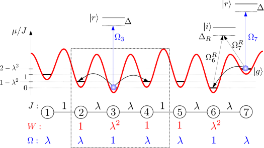
Figure S5: Scheme of the possible experimental implementation of the M₁ model for a generic $\lambda$. The pattern of tunneling amplitudes $J$, next-nearest neighbour interactions $W$ and the corresponding on-site Rydberg laser Rabi frequencies $\Omega$ is given at the bottom in black, red, blue respectively. The necessary periodicity can be achieved with a bi-chromatic optical lattice with ratio 1/3 between the lattice wavelengths. In order to realize the required tunneling amplitudes, one might use Raman assisted hoppings with Raman Rabi frequencies $\Omega^{R}_{i}$ and detunings $\Delta_{R}$ via an intermediate state $\ket{i}$. The dashed rectangle denotes the basic building block which, when repeated, constitutes the whole chain (with the appropriate boundary chemical potentials as indicated).

V.2.1 Effect of the interaction tails off-criticality

It is instructive to consider the effect of the dressed interaction beyond next-to-nearest neighbours. Using the pattern of the on-site Rabi frequencies $\Omega_{i}$ shown in Fig. S5 and the Eq. (S25) we get for the patterns of the next-to and the next-to-next-to nearest neighbours

$$\vec{\Omega} = \Omega(\lambda,\lambda,1,\lambda,\lambda,1,\ldots)$$

$$\Rightarrow$$

$$\vec{W}(2r_{0}) = (W_{1}(2r_{0}),W_{2}(2r_{0}),W_{3}(2r_{0}),W_{4}(2r_{0}),\ldots)\propto\Omega^{4}(\lambda^{2},\lambda^{4},\lambda^{2},\lambda^{2},\ldots)$$

$$\vec{W}(3r_{0}) = (W_{1}(3r_{0}),W_{2}(3r_{0}),W_{3}(3r_{0}),\ldots)\propto\Omega^{4}(\lambda^{4},\lambda^{4},1,\ldots)$$ (S27)

It is thus apparent that for sufficiently small $\lambda$, the neglected interactions beyond next-to-nearest neighbours $W(3r_{0})$ will become dominant (the “1” terms in $\vec{W}(3r_{0})$) and cannot be neglected anymore. We would like to emphasize that this observation does not affect the discussion of the kink dynamics at the critical point $\lambda=1$ in the main text, but it clearly limits the exploration of the off-critical regime. To quantify the effect of the long-range interactions we consider system sizes $L=3l$ featuring a unique ground state, cf. the Table 1, and the dressed Hamiltonian (S26) which now includes all the terms beyond $W(2r_{0})$

$$JH_{Q}^{\rm long-range}=JH_{Q}+\sum_{n=3}^{L-1}\sum_{i=1}^{L-n}W_{i}(nr_{0})n_{i}n_{i+n}$$ (S28)

Let us denote by $\ket{\psi_{\rm long-range}}$, $\ket{\psi_{0}}$ the ground states of (S28) and (S26), $\ket{\psi_{0}}$ corresponding to the notation used in Sec. III. In Fig. S6a we show the fidelity

$$F=|\braket{\psi_{\rm long-range}}{\psi_{0}}|$$ (S29)

vs. $\lambda$ for various system sizes (gray lines). It is apparent that the inclusion of the long-range tails limits the exploration of the off-critical regime to $\lambda$ asymptotically approaching 1 in the limit of infinite system sizes. Panes (b,c) of Fig. S6 then show the finite-size scaling of the value of $\lambda$ corresponding to maximum slope (largest gradient) of the fidelity

$$\lambda_{\rm max-slope}=\max\limits_{\lambda}\left(\partial_{\lambda}F(\lambda)\right),$$ (S30)

pane (b), and the error $1-F$ in the ground state fidelity at criticality, pane (c) (gray lines).

In the following section we discuss how to significantly suppress the unwanted effect of the tails of the interaction using doubly-dressed Rydberg potential. This not only allows to extend the region of high fidelity ground states to smaller $\lambda$ and larger system sizes but also achieves tenfold improvement in the $W(2r_{0})/W(3r_{0})$ ratio over the single dressing scheme.

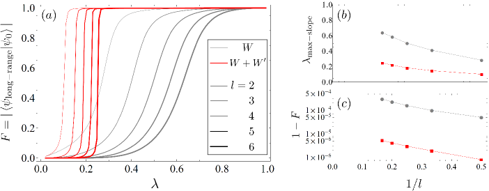
Figure S6: (a) Fidelity (S29) vs. $\lambda$ for the single and double dressing schemes (gray and red lines respectively) corresponding to the dressed potentials $W$ and $W_{\rm tot}=W+W^{\prime}$, see Sec. V.3. The line thickness indicates varying system size from $l=2$ (thin lines) to $l=6$ (thick lines). (b) Finite-size scaling of $\lambda_{\rm max-slope}$, Eq. (S30), corresponding to the largest gradient of the fidelity in (a) for the single (gray) and double (red) dressing scheme. (c) Finite-size scaling of the error $1-F$ at criticality ($\lambda=1$) for the single (gray) and double (red) dressing scheme.

V.3 Improving the scheme using double dressing

The idea behind the improvement is to suppress the long-range tail $W_{i}(nr_{0})$, $n>2$, of the dressed potential (S25) by a second potential with asymptotically the same behaviour in the long separation limit, but with opposite sign. Specifically, from (S25) we have

$$\left.W_{i}(nr_{0})\right|_{n\rightarrow\infty}=\frac{(\Omega_{i}\Omega_{i+n})^{2}}{\Delta^{4}}V(nr_{0}).$$ (S31)

With a slight abuse of notation, let us denote the quantities corresponding to the second potential with a prime (not to be confused with (S23)). We thus require

$$\left.W_{i}(nr_{0})\right|_{n\rightarrow\infty}=-\left.W^{\prime}_{i}(nr_{0})\right|_{n\rightarrow\infty}\;\;\Rightarrow\;\;\Omega^{\prime}=\Omega\left|\frac{\Delta^{\prime}}{\Delta}\right|\left|\frac{C_{6}}{C_{6}^{\prime}}\right|^{\frac{1}{4}},$$ (S32)

where $\Omega^{(^{\prime})}$ is the amplitude of the pattern of the on-site Rabi frequencies, $\vec{\Omega}^{(^{\prime})}=\Omega^{(^{\prime})}(\lambda,\lambda,1,\ldots)$, and we recall that the bare Rydberg interaction reads $V^{(^{\prime})}(nr_{0})=C^{(^{\prime})}_{6}/(nr_{0})^{6}$ and $C_{6}^{{}^{\prime}}<0$. The Eq. (S32) thus represents a condition for the amplitude of the second dressing Rabi frequency with other parameters given. We also note that in order to avoid the resonance $\Delta^{\prime}+V^{\prime}(r)=0$, which leads to the vanishing denominator in (S25) and can be exploited for instance to realize a spin model featuring both attractive and repulsive interaction Lan et al. (2015), we take $\Delta^{\prime}<0$.

The considered construction is allowed by an appropriate choice of the additional Rydberg state which features attractive rather than repulsive interaction. Specifically, in addition to the $\ket{{\rm nS}}$ state of ${}^{6}{\rm Li}$ which has $C_{6}>0$ we choose the $\ket{{\rm nD}_{\frac{3}{2}}}$ state with $C_{6}^{\prime}<0$. An example of $W$, $W^{\prime}$ and $W+W^{\prime}$ is shown in Fig. S7 as solid red, blue and black lines respectively. Here we have assumed $\lambda=1$, i.e. $\Omega_{i}=\Omega\;\forall i$ for the sake of simple illustration and considered the Rydberg level $\ket{74{\rm D}_{\frac{3}{2}}}$ with $C_{6}^{\prime}=-6\,005\,{\rm GHz}\cdot\mu{\rm m}^{6}$ Šibalić et al. (2017, ) in addition to the $\ket{84{\rm S}}$ one. Clearly, the details of the resulting potential depend on the precise choice of the parameters in the now extended parameter space spanned by $\Omega,\Delta,C_{6},\Delta^{\prime},C_{6}^{\prime}$ (with $\Omega^{\prime}$ given by (S32)). The detailed exploration of this parameter space goes beyond the scope of the present work, however we note that the resulting choice is typically a compromise between maximizing the energy scale $W_{\rm tot}(2r_{0})$ and maximizing the ratios $W_{\rm tot}(r_{0})/W_{\rm tot}(2r_{0})$ and $W_{\rm tot}(2r_{0})/W_{\rm tot}(3r_{0})$ which characterize the blockade and the suppression of the long-range tails respectively. Here $W_{\rm tot}=W+W^{\prime}$ is the total dressed potential. To illustrate this, the inset of Fig. S7 shows the detail of the potential for the next-to and next-to-next-to nearest neighbours for $\ket{84{\rm D}_{\frac{3}{2}}}$ with $C_{6}^{\prime}=-24\,200\,{\rm GHz}\cdot\mu{\rm m}^{6}$ Šibalić et al. (2017, ) (dashed line) in addition to the potential stemming from the $\ket{74{\rm D}_{\frac{3}{2}}}$ state (solid line). We get for these two situations

$$\ket{84{\rm S}},\ket{74{\rm D}_{\frac{3}{2}}}:\;(W_{\rm tot}(2r_{0})=J,W_{\rm tot}(r_{0})/W_{\rm tot}(2r_{0}),W_{\rm tot}(2r_{0})/W_{\rm tot}(3r_{0})) \approx (1\,{\rm kHz},74,94)$$

$$\ket{84{\rm S}},\ket{84{\rm D}_{\frac{3}{2}}}:\;(W_{\rm tot}(2r_{0})=J,W_{\rm tot}(r_{0})/W_{\rm tot}(2r_{0}),W_{\rm tot}(2r_{0})/W_{\rm tot}(3r_{0})) \approx (2.4\,{\rm kHz},35,56).$$ (S33)

which illustrate the point discussed, i.e. the increase of the effective Hamiltonian energy scale $W_{\rm tot}(2r_{0})$ at the expense of reducing the quality of the blockade and the suppression of the interaction tails. In particular the values $(W_{\rm tot}(r_{0})/W_{\rm tot}(2r_{0}),W_{\rm tot}(2r_{0})/W_{\rm tot}(3r_{0}))$ should be contrasted with the values 21 and 11 respectively of the single dressing scheme. We thus see that both of these ratios can be enhanced by a factor 5-10 with the double dressing scheme.

Two minor comments are in order. Firstly, as $\Omega^{\prime}$ is constrained by the Eq. (S32) one has to check whether it still satisfies $\Omega^{\prime}\ll|\Delta^{\prime}|$ required for the perturbative description to hold. Since we have chosen $|\Delta^{\prime}|\approx|\Delta|$ and we have $|C_{6}^{\prime}|>|C_{6}|$, it follows from (S32) that it is indeed the case (specifically, for the chosen value $\Delta^{\prime}=-500\,{\rm MHz}$ we get $|\Omega^{\prime}/\Delta^{\prime}|\approx 1/17.5$ with $\Omega^{\prime}\approx 2\pi\times 4.5\,{\rm MHz}$ for $\ket{74{\rm D}_{\frac{3}{2}}}$ and $|\Omega^{\prime}/\Delta^{\prime}|\approx 1/24.5$ with $\Omega^{\prime}\approx 2\pi\times 3.2\,{\rm MHz}$ for $\ket{84{\rm D}_{\frac{3}{2}}}$). Secondly, one should also verify whether the separation between adjacent Rydberg levels is larger than the considered detunings so that one still selectively addresses the target Rydberg state. For the range $n\sim 70-80$ of the principal quantum numbers, the typical separation between adjacent $\ket{{\rm nS}}-\ket{{\rm(n+1)S}}$ and $\ket{{\rm nD}}-\ket{{\rm(n+1)D}}$ states is of the order of 10 GHz which is well above the values of the considered detunings $|\Delta|,|\Delta^{\prime}|\sim 0.5\,{\rm GHz}$.

Finally, let us go back to the discussion of Sec. V.2.1 about the effect of the long-range tails of the interactions as quantified by the ground state fidelity of the supersymmetric Hamiltonian (S26). The fidelity, $\lambda_{\rm max-slope}$ and the ground state error $1-F$ at criticality corresponding to the doubly-dressed potential are shown in red in Fig. S6. We see that the double dressing scheme significantly improves over the single dressing one reducing $\lambda_{\rm max-slope}$ by a factor of $\gtrsim 3$ and the error at criticality by two orders of magnitude for the same system size.

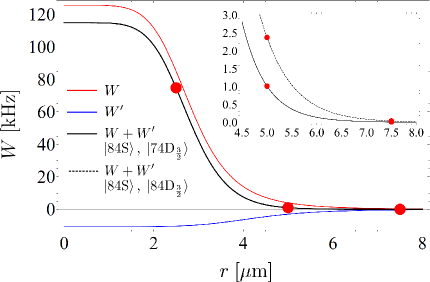
Figure S7: The doubly dressed potential $W_{\rm tot}=W+W^{\prime}$ (solid black line) composed of the repulsive $W$ (solid red line) and attractive $W^{\prime}$ (solid blue line) as a function of the distance $r$. The red circles indicate the potential at the positions of the atoms spaced by $r_{0}=2.5\,\mu{\rm m}$. Parameters used for $W$ are that of Fig. 1, i.e. $\Omega=2\pi\times 10\,{\rm MHz}$, $\Omega/\Delta=1/10$, $C_{6}=645\,{\rm GHz}\cdot\mu{\rm m}^{6}$ corresponding to the state $\ket{84{\rm}{\rm S}}$ of ${}^{6}{\rm Li}$. Parameters used for $W^{\prime}$ are $\Delta^{\prime}=-500\,{\rm MHz}$, $C_{6}^{\prime}=-6\,005\,{\rm GHz}\cdot\mu{\rm m}^{6}$ for $\ket{74{\rm D}_{\frac{3}{2}}}$ with $\Omega^{\prime}=2\pi\times 4.5\,{\rm MHz}$ given by the Eq. (S32). The inset shows, in addition to $W_{\rm tot}$ of the main plot (solid black line), $W_{\rm tot}$ corresponding to taking $\ket{84{\rm D}_{\frac{3}{2}}}$ instead of $\ket{74{\rm D}_{\frac{3}{2}}}$ for the second Rydberg state with parameters $C_{6}^{\prime}=-24\,200\,{\rm GHz}\cdot\mu{\rm m}^{6}$ yielding $\Omega^{\prime}=2\pi\times 3.2\,{\rm MHz}$ (dashed black line).

V.4 Arbitrary number of dressing potentials

In this section we generalize the above considerations and address the following question: Provided an arbitrary number of dressing potentials $W$ of the form (S24) is available, is it possible to generate a total potential $W_{\rm tot}=\sum_{\{W\}}W$ which matches the target potential implementing the supersymmetric model, i.e. satisfying (we again focus on the critical case $\lambda=1$ for simplicity)

$$\frac{W_{\rm tot}(r_{0})}{W_{\rm tot}(2r_{0})} \rightarrow\infty\;\;\;\text{(perfect blockade)}$$ (S34a)

$$\frac{W_{\rm tot}(2r_{0})}{W_{\rm tot}(nr_{0})} \rightarrow\infty\;\;\text{for}\;n>2\;\;\;\text{(no interaction tails)}$$ (S34b)

with $W(2r_{0})$ the relevant energy scale? To this end we first write the $j$-th potential (S24) in a customary form as

$$W(r,\rho_{j}) =A_{j}\frac{1}{(\rho_{j}r)^{6}+1}$$ (S35a)

$$A_{j} =\frac{2\left.\Omega^{(j)}\right.^{4}}{\left.\Delta^{(j)}\right.^{3}}$$ (S35b)

$$\rho_{j} =\left(\frac{2\Delta^{(j)}}{C^{(j)}_{6}}\right)^{\frac{1}{6}},$$ (S35c)

where $A_{j}$ is the potential amplitude and $\rho_{j}$ the characteristic inverse radius. The functions $W(r,\rho_{j})$ constitute a set on which we wish to decompose our target potential $W_{\rm target}$. If we allow for an infinite such set with smoothly varying $A$ and $\rho$, we can formulate this requirement as

$$W_{\rm target}(r)=\int_{0}^{\infty}{\rm d}\rho\,W(r,\rho)A(\rho).$$ (S36)

This is nothing but the inhomogeneous Fredholm equation of the first kind with kernel $W(r,\rho)$ and an unknown function $A(\rho)$. In order to proceed, we need to specify the target potential $W_{\rm target}$, which has to be chosen to satisfy the conditions (S34). Motivated by the fact that at long distances the dressed potentials decay as $r^{-6}$, we consider a function

$$\frac{W_{\rm target}(nr_{0})}{W_{\rm target}(2r_{0})}=\begin{cases}s\;\;\;\text{for}\;\;\;n=1\\ 1\;\;\;\text{for}\;\;\;n=2\\ \frac{1}{s}\;\;\;\text{for}\;\;\;n=3\\ \frac{1}{s}\left(\frac{3}{n}\right)^{6}\;\;\;\text{for}\;\;\;n>3,\end{cases}$$ (S37)

where $s$ is the suppression factor such that $W_{\rm target}(r_{0})/W_{\rm target}(2r_{0})=W_{\rm target}(2r_{0})/W_{\rm target}(3r_{0})=s$ and
$W_{\rm target}(nr_{0})/W_{\rm target}((n+1)r_{0})=(n+1)^{6}/n^{6}$. One obtains the ideal supersymmetric potential in the limit $s\rightarrow\infty$.

Next, we need to determine the potential amplitudes $A(\rho)$. To proceed, we consider a discrete set of separations $\{r_{i}\}$ and inverse characteristic radii $\{\rho_{j}\}$ such that we get from the Fredholm equation (S36)

$$W_{\rm target}(r_{i})=\sum_{j}W(r_{i},\rho_{j})A(\rho_{j}).$$ (S38)

The equation (S38) is thus a matrix equation for the amplitudes $A$ which can be inverted using pseudoinverse $W^{+}$ as

$$A=W^{+}W_{\rm target}.$$ (S39)

Here we consider the pseudoinverse since we are dealing in general with a rectangular rather than a square matrix $W(r_{i},\rho_{j})$. In fact, even when dealing with a square matrix, it might not be invertible (and in general is not). Since we use a finite set $\{r_{i}\}$ in (S38), the resulting total potential

$$W_{\rm tot}(r)=\sum_{j}W(r,\rho_{j})A(\rho_{j})$$ (S40)

will differ from $W_{\rm target}$ for a general $r\not\in\{r_{i}\}$.

It would be desirable to investigate the mathematical properties of (S36),(S38) in detail. For the purpose of demonstrating that such approach can yield arbitrary suppression $s$, yielding the ideal potential satisfying Eqs. (S34), we consider specific examples illustrated in Fig. S8. We refer the reader to the caption for all relevant details.

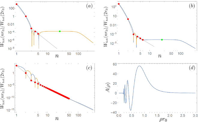
Figure S8: The total potential $W_{\rm tot}$ (blue and yellow solid lines in (a-c)), Eq. (S40), obtained from the discrete version of the Fredholm equation (S38) for suppression factors $s=10^{3}$ (a,c) and $s=10^{5}$ (b). The red circles indicate the set $\{r_{i}\}$ of atomic distances used in (S38). In (a,b) [(c)] we use 8 [200] equally spaced inverse radii $\rho_{j}$ from the interval $\rho_{j}r_{0}\in[0.01,2]$ [$\rho_{j}r_{0}\in[0.01,3]$]. Since we use the logarithmic plot, the blue (yellow) colour indicate the positive (negative) part of $W_{\rm tot}$. One can see from (a-c) that the total potential matches the specified points $\{r_{i}\}$ but deviates from $W_{\rm target}$, Eq. (S37) (solid gray line), for $r\not\in\{r_{i}\}$. In particular, one has to verify that the condition (S34b) is satisfied for large $r$. In (a), (b) we get $W_{\rm tot}(2r_{0})/W_{\rm tot}(25r_{0})\approx-5200$ and $6\cdot 10^{6}$ respectively, where the reference point $n=25$ is indicated by the green circle. Furthermore, in (d) we show the form of the amplitude function $A(\rho_{j})$ for the parameters used in (c).

The results presented in the Fig. S8 indicate that arbitrary suppression $s$, and thus the ideal supersymmetric potential corresponding to the next-to-nearest neighbour interaction (S34) can be achieved in principle, provided a sufficient number of suitable dressing potentials is available. To assess an experimental feasibility of such approach would however require a detailed study of available van der Waals couplings provided by the Rydberg levels and realistic Rabi frequencies and detunings. More involved dressing schemes would also increase the decoherence rates as we discuss in the next section. While such a detailed study of experimental feasibility goes beyond the scope of the present work, the possibility of engineering step-like potentials through multiple dressings remains an interesting opening which it might be interesting to address in the future.

V.5 Coherent evolution

In practice, any experiment is prone to detrimental effects, such as decoherence due to off-resonant scattering from the Rydberg state. On the one hand, one can reduce the scattering, the rate of which $\propto(\Omega/\Delta)^{2}$, by reducing $\Omega/\Delta$. On the other hand, to limit the influence of such scattering, it is desirable to reduce the time of the experiment, by increasing the energy scale of $H_{\rm Ry}$. Since $J=W(2r_{0})\propto\Omega^{4}/\Delta^{3}$, it can be achieved by increasing $\Omega$ and reducing $\Delta$ while still in the perturbative regime $\Omega/\Delta\ll 1$. For this reason, to weigh between these two effects, we choose as a figure of merit the achievable system size, for which $\ket{K_{1}}$ traverse the chain coherently in time $t=LT_{c}$, where $T_{c}=1/(3v_{F}W(2r_{0}))$ is the characteristic propagation time between lattice sites. To obtain $L_{\rm max}$, $t$ should be equated with the effective decay time $\tau=1/\gamma$, where $\gamma\cong L/3\gamma_{0}(\Omega/\Delta)^{2}$ is the sum of $\approx L/3$ individual atomic far-detuned decay rates Wüster et al. (2011). Combining these expressions we get

$$L_{\rm max}=3\sqrt{\frac{\tau_{0}v_{F}W(2r_{0})}{\left(\frac{\Omega}{\Delta}\right)^{2}}}=3\Omega\sqrt{\frac{2\tau_{0}v_{F}}{\Delta\left(1+\frac{2\Delta}{V_{2}}\right)}}.$$ (S41)

Fig. S9 shows $L_{\rm max}$ vs. $\Delta/\Omega$ for the state $\ket{84{\rm S}}$ of ⁶Li and parameters used in the main text, $C_{6}=645\,{\rm GHz}\cdot\mu{\rm m}^{6}$, $r_{0}=2.5\,\mu{\rm m}$. It is apparent from the Figure that system sizes of the order of 100 sites might be achievable for realistic parameters. While this is encouraging, it is known that the dressing schemes are sensitive to detrimental effects, such as line broadening Goldschmidt et al. (2016) leading to avalanche dephasing Boulier et al. (2017); Young et al. (2018). It has been suggested, however, that these effects can be mitigated by cooling to reduce the black-body radiation or quenching the contaminant states Boulier et al. (2017).

Next, in analogy to the derivation of Eq. (S41) we can derive the scaling of the system size taking into account both adiabatic preparation, cf. Sec. III, and the subsequent time evolution. We note that the estimation Eq. (S41) holds for any $\lambda$, in which case $v_{F}$ should be replaced by $v_{\rm max}(\lambda)$.

To proceed, we quantify the preparation time as a multiple $\kappa$ of the inverse spectral gap,

$$T=\frac{\kappa}{\Delta_{sg}}.$$ (S42)

Working at criticality, we use the formula for finite size scaling of the gap Huijse (2011)

$$\Delta_{sg}\approx\frac{2\pi E_{\rm SCFT}3v_{F}W(2r_{0})}{L},$$ (S43)

where $E_{\rm SCFT}=1/3\;(2/3)$ for $L=3l+1$ ($L=3l$) respectively. We write the dispersive decay rates of $l\approx L/3$ atoms as

$$\Gamma=\frac{L}{3}\frac{1}{\tau_{0}}\left(\frac{\Omega}{\Delta}\right)^{2}\bar{p},\qquad\gamma=\frac{L}{3}\frac{1}{\tau_{0}}\left(\frac{\Omega}{\Delta}\right)^{2},$$ (S44)

where $\bar{p}$ stands for the average probability of being in the Rydberg state during the adiabatic sweep and depends on the form of the sweep. For the function (S7) it is taken to be

$$\left(\frac{\Omega}{\Delta}\right)^{2}\bar{p}=\frac{1}{T}\int_{0}^{T}{\rm d}t\,\left(\frac{\Omega(t)}{\Delta}\right)^{2}=\left(\frac{\Omega}{\Delta}\right)^{2}\frac{1}{T}\int_{0}^{T}{\rm d}t\,\sqrt{{\mathcal{F}}(t)}=\left(\frac{\Omega}{\Delta}\right)^{2}\frac{2}{\pi}\;\rightarrow\;\bar{p}=\frac{2}{\pi},$$ (S45)

where the ramping of the Hamiltonian is implemented by tuning the Rabi frequency so that ${\mathcal{F}}(t)\propto\Omega(t)^{4}$ and correspondingly for the tunnelings $J(t)$. Setting

$$\Gamma T+\gamma t=1$$ (S46)

and recalling that $t=LT_{c}=L/[3v_{F}W(2r_{0})]$, we can express $L$ after substituting (S42-S44) to (S46) as

$$L_{\rm max}=3\Omega\sqrt{\frac{\tau_{0}2v_{F}}{\Delta\left(1+\frac{2\Delta}{V_{2}}\right)}\frac{1}{\left(\frac{1}{2\pi}E_{\rm SCFT}\kappa\bar{p}+1\right)}}.$$ (S47)

We note that setting $\kappa=0$ corresponds to ignoring the preparation stage and we recover the formula (S41). Similarly, ignoring the time evolution, as in the case of the preparation of the ground states for chains with $L=3l$, amounts to neglecting the “+1” term in the second denominator.

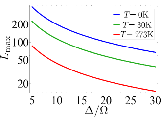
Figure S9: Maximum chain length $L_{\rm max}$ for a coherent evolution using Rydberg state $\ket{84{\rm S}}$ of ${}^{6}{\rm Li}$ for temperatures $T=(0,30,273)\,{\rm K}$ (blue, green, red) corresponding to $\tau_{0}=(8.6,2.8,0.42)\,{\rm ms}$ Šibalić et al. (2017, ).

V.6 Energy scales and quality of the approximations

Estimates of energy scales. It is apparent from the previous sections that engineering the supersymmetric Hamiltonian is a tradeoff between a number of requirements. On one hand one wishes to maximize the energy scales, namely the dressing Rabi frequency $\Omega$, which determines the interaction Eq. (S24) to overcome the decoherence, cf. Eq. (S47). Tuning the Hamiltonian to the supersymmetric point $J=W(2r_{0})$, it also maximizes the tunneling rate, cf. Eq. (S26). Same effects result from reducing $\Delta$.

On the other hand, one wishes to minimize $\Omega/\Delta$ to be well in the adiabatic approximation regime, where the flat-top interaction potential (S24) remains valid, the population in the Rydberg state is negligible and where the Rydberg Hamiltonian, Eq. (6) of the main text, approaches the supersymmetric one.

While precise quantification of this trade-off goes beyond the scope of the present article, for illustration purposes it is instructive to consider specific example. Focusing on fermionic ${}^{6}{\rm Li}$, the choice of the Rydberg state $\ket{84{\rm S}}$ used in the main text is motivated by the maximization of the Rydberg state lifetime to overcome the decoherence, cf. Eq. (S47), as (at zero temperature) $\tau_{0}\propto\left.n^{*}\right.^{3}$, where $n^{*}$ is the effective principal quantum number accounting for a quantum defect Gallagher (2005). The associated Van der Waals coefficient $C_{6}=645\;{\rm GHz}\cdot\mu{\rm m}^{6}$ determines the Rydberg interaction energy. Choosing $\Omega=2\pi\times 10$ MHz and $\Omega/\Delta=1/10$ as experimentally sensible values, the lattice constant $r_{0}=2.5\;\mu{\rm m}$ is determined to satisfy the hierarchy $W(r_{0})\gg W(2r_{0})\gg W(3r_{0})$. This then finally determines the actual energy scale of the Hamiltonian at the supersymmetric point $J=W(2r_{0})\approx 4\;{\rm kHz}$.

In the main text, we have focused mainly on the critical case $\lambda=1$. This was motivated by the relative experimental simplicity compared to the off-critical one described in Sec. V.2, but also by its prominence, since at criticality the propagating kinks reach their maximum velocity, the Fermi velocity $v_{F}$. In this case the chemical potential $\mu$ in Eq. (S26) contributes a uniform global offset and can be thus dropped everywhere but at the boundaries, where $\mu_{1}=\mu_{L}=J$.

With this, we can now enquire about the experimental feasibility of such scenario. Our construction relies on the tight-binding approximation for atoms tunneling in the optical lattice. For lattice potentials of the form $V(x)=V_{0}/2\cos(2kx)$ this occurs in the limit $V_{0}/E_{r}\gg 1$, where $E_{r}=(\hbar k)^{2}/(2m)$ is the recoil energy, $m$ the atom mass and $k=2\pi/\lambda$ the lattice wavevector. In the tight-binding regime, the tunneling rate is given by Arzamasovs and Liu (2017)

$$J/E_{r}=\frac{4}{\sqrt{\pi}}\left(\frac{V_{0}}{E_{r}}\right)^{\frac{3}{4}}{\rm e}^{-2\sqrt{\frac{V_{0}}{E_{r}}}}$$ (S48)

and the band width $\Delta E=4J$. Furthermore, taking a harmonic approximation for the minima of the potential $V(x)$, one can identify the corresponding harmonic oscillator frequency separating the ground and the first excited state as $\omega=\sqrt{2V_{0}k^{2}/m}$. This indicates the relevant energy scale for the temperature of the atoms, namely $k_{\rm B}T\ll\omega$ in order to avoid thermal excitations of the higher bands of the lattice. Put together we thus require $V_{0}\gg E_{r}$ and $\Delta E,k_{\rm B}T\ll\omega$.

The above parameters fix the tunneling rate $J\approx 4\;{\rm kHz}$, which implies $V_{0}\approx 5.5\,E_{r}$ (for $\lambda=2r_{0}=5\,\mu{\rm m}$ of the optical lattice laser light) and $\omega\approx 2\pi\times 6\;{\rm kHz}$ corresponding to $\hbar\omega/k_{\rm B}\approx 0.3\;\mu{\rm K}$. To this end we note that temperatures of order $O(10\;{\rm nK})$ have been achieved when cooling fermions in optical lattices Taie et al. (2012); Ozawa et al. (2018); Taie et al. (2020). Clearly, the value $V_{0}/E_{r}\approx 5.5$ puts in question the appropriateness of the tight-binding approximation. One way to ensure its applicability is to increase $V_{0}/E_{r}$, reducing however the tunneling rate significantly. For instance for $V_{0}/E_{r}=40$ we get $J=6\;{\rm Hz}$. To remedy this, one could implement the Raman assisted hopping as suggested in Fig. S5 in the context of the off-critical implementation of the ${\rm M}_{1}$ model, leading to $J\propto\left.\Omega^{R}\right.^{2}/\Delta_{R}$.

Quality of the approximations. In the proposed quantum simulation of the supersymmetric lattice Hamiltonian, we have made two crucial approximations, namely we have adiabatically eliminated the Rydberg states, cf. Sec. V.1 and neglected the long range tails of the dressed interaction beyond next-to-nearest neighbours. The former approximation effectively neglects a finite population in the Rydberg state which results in photon scattering with associated energy scale $\gamma\propto\gamma_{0}(\Omega/\Delta)^{2}$, cf. Sec. V.5, while the energy scale of the latter is $W(3r_{0})$. These two scales then set a bound on the times where the approximations remain valid. Importantly, one also requires coherent evolution up to times $tJ/l\sim O(1)$, where $J=W(2r_{0})$, to see the effects of the (s)kink propagation.

Here we specifically focus on evaluating the effect of neglecting the tails of the interaction versus neglecting the scattering. We further parametrize $W(nr_{0})=w_{n}\Omega^{4}/\Delta^{3}$ and ask what is the effect of both for a given time $tJ$. We get for the scattering and neglecting the tails respectively

$$\frac{t\gamma}{tJ}\propto\frac{1}{w_{2}}\frac{\Delta}{\Omega}\frac{\gamma_{0}}{\Omega},\;\;\frac{tW(3r_{0})}{tJ}=\frac{W(3r_{0})}{W(2r_{0})}.$$ (S49)

The ratio $W(3r_{0})/W(2r_{0})\ll 1$ by construction. In comparison, $\Delta\gamma_{0}/(w_{2}\Omega^{2})\approx 290$ for the parameters used in the main text, i.e. $\Omega=2\pi\times 10\,{\rm MHz}$, $\Omega/\Delta=1/10$, $C_{6}=645\,{\rm GHz}\cdot\mu{\rm m}^{6}$, $r_{0}=2.5\,\mu{\rm m}$ and taking $\tau_{0}=1/\gamma_{0}=8.6\,{\rm ms}$ corresponding to zero temperature lifetime of $\ket{84{\rm}{\rm S}}$ state of ${}^{6}{\rm Li}$. It is thus clear that the off-resonant scattering is the dominant limiting factor for the coherent evolution. Furthermore, this trend will become even more pronounced in the double dressing scheme discussed in Sec. V.3, which further reduces the ratio $W(3r_{0})/W(2r_{0})$ and increases the scattering due to the off-resonant coupling to the additional Rydberg state. This is indeed compatible with the time dynamics generated by the Rydberg Hamiltonian with interactions truncated beyond next-to-nearest neighbour (gray line in Fig. 3c). In this case, the only discrepancy with respect to the dynamics generated by the supersymmetric Hamiltonian (blue dashed line in Fig. 3c) comes from the leakage to the Rydberg state. While this increases with increasing $\Omega/\Delta$, the overall optimization is dictated by the requirements in Eq. (S49), namely it is favorable to increase $\Omega/\Delta$ while maximizing $\Omega$, cf. Sec. V.5.

In summary, while further optimization is in principle possible, for realistic parameters the effect of omitting the tails remains negligible in comparison with the leakage of the atom population to the Rydberg state and the associated scattering. As mentioned in the main text, a promissing avenue to overcome this difficulty is to use cold molecules instead of Rydberg atoms Büchler et al. (2007); Baranov et al. (2012). These are particularly interesting as they provide permanent or electric-field induced dipole moment, which is typically of order 1 Debye corresponding to the interaction energy of 10 kHz for $1\,\mu{\rm m}$ separation Carr et al. (2009); Baranov et al. (2012); Balakrishnan (2016), scale comparable to the present study. This would provide the blockade without the need of dressing to the optically excited state avoiding thus the decoherence due to off-resonant scattering.

Symmetry considerations. Let us recap the effects of the finite energy scales from the point of view of the (super)symmetry of the target Hamiltonian. As discussed in the previous paragraph, for the relevant parameter regime, the imperfect blockade $W(r_{0})/W(2r_{0})<\infty$ dominates over the effect of the interaction tails $W(nr_{0}),n>2$, cf. Eq. (S28), and both represent a weak breaking of the supersymmetry.

In order to quantify the effect of the tails in the limit of large system sizes one could treat the effects of the $W(nr_{0})$ terms, $n>2$, perturbatively (as suggested in a similar context in Lesanovsky and Katsura (2012)) or using large-scale numerical simulations for real time evolution such as the DMRG Paeckel et al. (2019) or neural networks Carleo and Troyer (2017) based methods. Similarly, one could perform a systematic study of the imperfect blockade by replacing the projectors $P_{i}$ in the definition of the supercharges $Q$, cf. (S26), by $P_{i}\rightarrow P_{i}+\eta n_{i}$, where $\eta=O(1/W(r_{0}))$ Lesanovsky and Katsura (2012) and simultaneous deformation of $H_{Q}$ from the supersymmetric point with a potential $\sum_{i}W(r_{0})n_{i}n_{i+1}$ to account for the nearest-neihbour interaction. However, such detailed analysis is beyond the scope of the present work.

Importantly, we note that $H_{Q}$, Eq. (S26), is recovered from the parent Rydberg Hamiltonian (6) in the limit of $W(r_{0})/W(2r_{0}),W(2r_{0})/W(nr_{0})\rightarrow\infty,\;\forall n>2$. This is reminiscent of a situation encountered in the early proposals Zohar et al. (2012); Banerjee et al. (2012) of the cold atom based quantum simulators of lattice gauge theories (LGT). There, the local Hamiltonian symmetry corresponds to the Gauss law which was recovered only asymptotically in the limit of infinite interaction strength of the parent Hubbard-like model from which the effective Hamiltonian corresponding to the LGT was derived. The engineering of the Gauss law has then been improved in Kasamatsu et al. (2013) by invoking the Higgs field, cf. also Haase et al. (2021); Paulson et al. (2020) for recent developments.

In this context, it would be interesting to explore alternative avenues for engineering the supersymmetric lattice Hamiltonians in order to recover the exact supersymmetry, for instance through the mapping to spin Hamiltonians as discussed in the Outlook of the main text.

References

- Suzuki (1993) M. Suzuki, Quantum Monte Carlo methods in condensed matter physics (World scientific, 1993).
- Gubernatis et al. (2016) J. Gubernatis, N. Kawashima, and P. Werner, Quantum Monte Carlo Methods (Cambridge University Press, 2016).
- Becca and Sorella (2017) F. Becca and S. Sorella, Quantum Monte Carlo approaches for correlated systems (Cambridge University Press, 2017).
- Orús (2014) R. Orús, Annals of Physics 349, 117 (2014).
- Montangero et al. (2018) S. Montangero, S. Montangero, and Evenson, Introduction to Tensor Network Methods (Springer, 2018).
- Zaanen et al. (2015) J. Zaanen, Y. Liu, Y.-W. Sun, and K. Schalm, Holographic duality in condensed matter physics (Cambridge University Press, 2015).
- Nicolai (1976) H. Nicolai, J. Phys. A 9, 1497 (1976).
- Fendley et al. (2003a) P. Fendley, K. Schoutens, and J. de Boer, Phys. Rev. Lett. 90, 120402 (2003a).
- Fendley et al. (2003b) P. Fendley, B. Nienhuis, and K. Schoutens, J. Phys. A 36, 12399 (2003b).
- Fu et al. (2017) W. Fu, D. Gaiotto, J. Maldacena, and S. Sachdev, Phys. Rev. D 95, 026009 (2017).
- Sannomiya et al. (2017) N. Sannomiya, H. Katsura, and Y. Nakayama, Phys. Rev. D 95, 065001 (2017).
- O’Brien and Fendley (2018) E. O’Brien and P. Fendley, Phys. Rev. Lett. 120, 206403 (2018).
- Grover et al. (2014) T. Grover, D. Sheng, and A. Vishwanath, Science 344, 6181 (2014).
- Huijse et al. (2014) L. Huijse, B. Bauer, and E. Berg, Phys. Rev. Lett. 114, 9 (2014).
- Yu and Yang (2010) Y. Yu and K. Yang, Phys. Rev. Lett. 105, 150605 (2010).
- Witten (1982) E. Witten, Nuclear Physics B 202, 253 (1982).
- van Eerten (2005) H. van Eerten, J. Math. Phys. 46, 123302 (2005).
- Fendley and Schoutens (2005) P. Fendley and K. Schoutens, Phys. Rev. Lett. 95, 046403 (2005).
- Chepiga et al. (2021) N. Chepiga, J. Minář, and K. Schoutens, arXiv:2105.04359 (2021).
- Browaeys and Lahaye (2020) A. Browaeys and T. Lahaye, Nature Physics 16, 132 (2020).
- Barredo et al. (2016) D. Barredo, S. De Léséleuc, V. Lienhard, T. Lahaye, and A. Browaeys, Science 354, 1021 (2016).
- Endres et al. (2016) M. Endres, H. Bernien, A. Keesling, H. Levine, E. R. Anschuetz, A. Krajenbrink, C. Senko, V. Vuletic, M. Greiner, and M. D. Lukin, Science 354, 1024 (2016).
- Barredo et al. (2018) D. Barredo, V. Lienhard, S. De Leseleuc, T. Lahaye, and A. Browaeys, Nature 561, 79 (2018).
- Wang et al. (2019) Y. Wang, S. Shevate, T. Wintermantel, M. Morgado, G. Lochead, and S. Whitlock, arXiv:1912.04200 (2019).
- Schauß et al. (2015) P. Schauß, J. Zeiher, T. Fukuhara, S. Hild, M. Cheneau, T. Macrì, T. Pohl, I. Bloch, and C. Groß, Science 347, 1455 (2015).
- Labuhn et al. (2016) H. Labuhn, D. Barredo, S. Ravets, S. De Léséleuc, T. Macrì, T. Lahaye, and A. Browaeys, Nature 534, 667 (2016).
- Bernien et al. (2017) H. Bernien, M. D. Lukin, H. Pichler, S. Choi, M. Greiner, V. Vuletić, A. Omran, H. Levine, S. Schwartz, A. Keesling, M. Endres, and A. S. Zibrov, Nature 551, 579 (2017).
- de Léséleuc et al. (2019) S. de Léséleuc, V. Lienhard, P. Scholl, D. Barredo, S. Weber, N. Lang, H. P. Büchler, T. Lahaye, and A. Browaeys, Science 365, 775 (2019).
- Helmrich et al. (2020) S. Helmrich, A. Arias, G. Lochead, T. Wintermantel, M. Buchhold, S. Diehl, and S. Whitlock, Nature 577, 481 (2020).
- Balewski et al. (2014) J. B. Balewski, A. T. Krupp, A. Gaj, S. Hofferberth, R. Löw, and T. Pfau, New Journal of Physics 16, 063012 (2014).
- Jau et al. (2016) Y.-Y. Jau, A. Hankin, T. Keating, I. Deutsch, and G. Biedermann, Nature Physics 12, 71 (2016).
- Zeiher et al. (2016) J. Zeiher, R. Van Bijnen, P. Schauß, S. Hild, J.-y. Choi, T. Pohl, I. Bloch, and C. Gross, Nature Physics 12, 1095 (2016).
- Arias et al. (2019) A. Arias, G. Lochead, T. M. Wintermantel, S. Helmrich, and S. Whitlock, Phys. Rev. Lett. 122, 053601 (2019).
- Huijse (2011) L. Huijse, J. Stat. Mech. 2011, P04004 (2011).
- Milsted et al. (2020) A. Milsted, J. Liu, J. Preskill, and G. Vidal, arXiv:2012.07243 (2020).
- Fendley and Hagendorf (2011) P. Fendley and C. Hagendorf, J. Stat. Mech. 2011, P02014 (2011).
- (37) See Supplemental Material for (i) particle densities of the critical ground states, (ii) (s)kink profiles and observables, (iii) state preparation, (iv) saddle point approximation and (v) details of the experimental implementation.
- Fokkema and Schoutens (2017) T. Fokkema and K. Schoutens, SciPost Phys. 3, 004 (2017).
- (39) J. Minář and K. Schoutens, In Preparation.
- Fendley and Hagendorf (2010) P. Fendley and C. Hagendorf, J. Phys. A 43, 402004 (2010).
- Henkel et al. (2010) N. Henkel, R. Nath, and T. Pohl, Phys. Rev. Lett. 104, 195302 (2010).
- Pupillo et al. (2010) G. Pupillo, A. Micheli, M. Boninsegni, I. Lesanovsky, and P. Zoller, Phys. Rev. Lett. 104, 223002 (2010).
- Šibalić et al. (2017) N. Šibalić, J. D. Pritchard, C. S. Adams, and K. J. Weatherill, Computer Physics Communications 220, 319 (2017).
- (44) N. Šibalić, J. D. Pritchard, C. S. Adams, and K. J. Weatherill, “Arc package,” https://arc-alkali-rydberg-calculator.readthedocs.io/en/latest/.
- Arzamasovs and Liu (2017) M. Arzamasovs and B. Liu, European Journal of Physics 38, 065405 (2017).
- Note (1) In order to be well in the deep lattice limit where the tight-binding approximation is applicable, one might further reduce . This would in turn reduce and the achievable . To overcome this limitation, one could use a Raman-assisted hopping as we discuss in Sup .
- Weimer et al. (2012a) H. Weimer, L. Huijse, A. Gorshkov, G. Pupillo, P. Zoller, M. Lukin, and E. Demler, in APS Division of Atomic, Molecular and Optical Physics Meeting Abstracts (2012).
- Weimer et al. (2012b) H. Weimer, L. Huijse, A. Gorshkov, G. Pupillo, P. Zoller, M. Lukin, and E. Demler, in 76. annual conference of the DPG and DPG Spring meeting 2012 (2012).
- Huijse et al. (2008) L. Huijse, J. Halverson, P. Fendley, and K. Schoutens, Phys. Rev. Lett. , 146406 (2008).
- Huijse et al. (2012) L. Huijse, D. Mehta, N. Moran, K. Schoutens, and J. Vala, New J. Phys. 14, 073002 (2012).
- Galanakis et al. (2012) D. Galanakis, C. L. Henley, and S. Papanikolaou, Phys. Rev. B 86, 195105 (2012).
- Surace et al. (2020) F. M. Surace, G. Giudici, and M. Dalmonte, arXiv:2003.11073 (2020).
- Gambetta et al. (2020) F. M. Gambetta, W. Li, F. Schmidt-Kaler, and I. Lesanovsky, Phys. Rev. Lett. 124, 043402 (2020).
- Büchler et al. (2007) H. Büchler, A. Micheli, and P. Zoller, Nature Physics 3, 726 (2007).
- Carr et al. (2009) L. D. Carr, D. DeMille, R. V. Krems, and J. Ye, New Journal of Physics 11, 055049 (2009).
- Baranov et al. (2012) M. A. Baranov, M. Dalmonte, G. Pupillo, and P. Zoller, Chemical Reviews 112, 5012 (2012).
- Balakrishnan (2016) N. Balakrishnan, The Journal of chemical physics 145, 150901 (2016).
- Pedersen et al. (2019) S. P. Pedersen, K. S. Christensen, and N. T. Zinner, Phys. Rev. Research 1, 033123 (2019).
- Roy et al. (2020) T. Roy, S. Hazra, S. Kundu, M. Chand, M. P. Patankar, and R. Vijay, Phys. Rev. Applied 14, 014072 (2020).
- Press et al. (2007) W. H. Press, S. A. Teukolsky, W. T. Vetterling, and B. P. Flannery, Numerical recipes 3rd edition: The art of scientific computing (Cambridge university press, 2007).
- Messiah (1999) A. Messiah, ed., Quantum Mechanics (Dover Publications, New York, 1999).
- Teufel (2003) S. Teufel, Adiabatic perturbation theory in quantum dynamics (Springer, 2003).
- Albash and Lidar (2018) T. Albash and D. A. Lidar, Rev. Mod. Phys. 90, 015002 (2018).
- Avron and Elgart (1998) J. E. Avron and A. Elgart, Phys. Rev. A 58, 4300 (1998).
- Rigolin and Ortiz (2012) G. Rigolin and G. Ortiz, Phys. Rev. A 85, 062111 (2012).
- Note (2) This is in contrast to the gap used in the main text in scenario (ii), which was the energy of the lowest excited state, i.e. its distance from the zero energy corresponding to the true ground state of the supersymmetric Hamiltonian on a chain with periodic boundaries. In the thermodynamic limit the lowest excited states become however equidistant as a consequence of the conformal symmetry and coincides with .
- Note (3) We numerically implement the time evolution using Crank-Nicholson discrete time-step evolution given by Press et al. (2007).
- Agarwal et al. (2018) K. Agarwal, R. N. Bhatt, and S. L. Sondhi, Phys. Rev. Lett. 120, 210604 (2018).
- Macrì and Pohl (2014) T. Macrì and T. Pohl, Phys. Rev. A 89, 011402 (2014).
- Note (4) Here it becomes apparent why we have introduced the site-dependent factor in the definition of the supercharge - this is required, for real, for the kinetic term to be negative. Another consequence of this choice is the appearance of triplets in the ground state . Conversely, the omission of the factor leads to positive kinetic term and singlets instead of triplets in .
- Jaksch and Zoller (2003) D. Jaksch and P. Zoller, New Journal of Physics 5, 56 (2003).
- Aidelsburger et al. (2011) M. Aidelsburger, M. Atala, S. Nascimbène, S. Trotzky, Y.-A. Chen, and I. Bloch, Phys. Rev. Lett. 107, 255301 (2011).
- Miyake et al. (2013) H. Miyake, G. A. Siviloglou, C. J. Kennedy, W. C. Burton, and W. Ketterle, Phys. Rev. Lett. 111, 185302 (2013).
- Lan et al. (2015) Z. Lan, J. c. v. Minář, E. Levi, W. Li, and I. Lesanovsky, Phys. Rev. Lett. 115, 203001 (2015).
- Wüster et al. (2011) S. Wüster, C. Ates, A. Eisfeld, and J. Rost, New J. Phys. 13, 073044 (2011).
- Goldschmidt et al. (2016) E. A. Goldschmidt, T. Boulier, R. C. Brown, S. B. Koller, J. T. Young, A. V. Gorshkov, S. L. Rolston, and J. V. Porto, Phys. Rev. Lett. 116, 113001 (2016).
- Boulier et al. (2017) T. Boulier, E. Magnan, C. Bracamontes, J. Maslek, E. A. Goldschmidt, J. T. Young, A. V. Gorshkov, S. L. Rolston, and J. V. Porto, Phys. Rev. A 96, 053409 (2017).
- Young et al. (2018) J. T. Young, T. Boulier, E. Magnan, E. A. Goldschmidt, R. M. Wilson, S. L. Rolston, J. V. Porto, and A. V. Gorshkov, Phys. Rev. A 97, 023424 (2018).
- Gallagher (2005) T. F. Gallagher, Rydberg atoms, 3 (Cambridge University Press, 2005).
- Taie et al. (2012) S. Taie, R. Yamazaki, S. Sugawa, and Y. Takahashi, Nature Physics 8, 825 (2012).
- Ozawa et al. (2018) H. Ozawa, S. Taie, Y. Takasu, and Y. Takahashi, Phys. Rev. Lett. 121, 225303 (2018).
- Taie et al. (2020) S. Taie, E. Ibarra-García-Padilla, N. Nishizawa, Y. Takasu, Y. Kuno, H.-T. Wei, R. T. Scalettar, K. R. Hazzard, and Y. Takahashi, arXiv:2010.07730 (2020).
- Lesanovsky and Katsura (2012) I. Lesanovsky and H. Katsura, Phys. Rev. A 86, 041601 (2012).
- Paeckel et al. (2019) S. Paeckel, T. Köhler, A. Swoboda, S. R. Manmana, U. Schollwöck, and C. Hubig, Annals of Physics 411, 167998 (2019).
- Carleo and Troyer (2017) G. Carleo and M. Troyer, Science 355, 602 (2017).
- Zohar et al. (2012) E. Zohar, J. I. Cirac, and B. Reznik, Phys. Rev. Lett. 109, 125302 (2012).
- Banerjee et al. (2012) D. Banerjee, M. Dalmonte, M. Müller, E. Rico, P. Stebler, U.-J. Wiese, and P. Zoller, Phys. Rev. Lett. 109, 175302 (2012).
- Kasamatsu et al. (2013) K. Kasamatsu, I. Ichinose, and T. Matsui, Phys. Rev. Lett. 111, 115303 (2013).
- Haase et al. (2021) J. F. Haase, L. Dellantonio, A. Celi, D. Paulson, A. Kan, K. Jansen, and C. A. Muschik, Quantum 5, 393 (2021).
- Paulson et al. (2020) D. Paulson, L. Dellantonio, J. F. Haase, A. Celi, A. Kan, A. Jena, C. Kokail, R. van Bijnen, K. Jansen, P. Zoller, et al., arXiv:2008.09252 (2020).
SUPPLEMENTAL MATERIAL