Unexpected crossovers in correlated random-diffusivity processes

Abstract

The passive and active motion of micron-sized tracer particles in crowded liquids and inside living biological cells is ubiquitously characterised by "viscoelastic" anomalous diffusion, in which the increments of the motion feature long-ranged negative and positive correlations. While viscoelastic anomalous diffusion is typically modelled by a Gaussian process with correlated increments, so-called fractional Gaussian noise, an increasing number of systems are reported, in which viscoelastic anomalous diffusion is paired with non-Gaussian displacement distributions. Following recent advances in Brownian yet non-Gaussian diffusion we here introduce and discuss several possible versions of random-diffusivity models with long-ranged correlations. While all these models show a crossover from non-Gaussian to Gaussian distributions beyond some correlation time, their mean squared displacements exhibit strikingly different behaviours: depending on the model crossovers from anomalous to normal diffusion are observed, as well as unexpected dependencies of the effective diffusion coefficient on the correlation exponent. Our observations of the strong non-universality of random-diffusivity viscoelastic anomalous diffusion are important for the analysis of experiments and a better understanding of the physical origins of "viscoelastic yet non-Gaussian" diffusion.

1 Introduction

Gaussianity is so fundamentally engrained in statistics that we almost take it for granted. The law of large numbers, merging into the central limit theorem (CLT) states that the sum of independent and identically distributed random variables with finite variance necessarily converges to a Gaussian ("normal") limit distribution. A prime example is the Gaussian probability density function (PDF) $P(x,t)=(4\pi Dt)^{-1/2}\exp(-x^{2}/[4Dt])$ of Brownian motion that also encodes the mean squared displacement (MSD) $\langle x^{2}(t)\rangle=2Dt$ with the diffusion coefficient $D$ [1].

The powerful CLT notwithstanding, a growing number of "Brownian yet non-Gaussian" processes are being reported. The original case was made by the Granick group for colloid motion along nanotubes and tracer diffusion in gels [2]. Similar behaviour is found for nanoparticle diffusion in nanopost arrays [3], diffusion of colloidal particles on fluid interfaces [4], and colloid motion on membranes as well as in suspension [5]. For further examples see [6, 7]. Typically, the shape of the PDF in these cases is exponential ("Laplace distribution"), while in some cases a crossover from exponential to Gaussian is observed beyond some correlation time [2]. An invariant exponential PDF can be explained by "superstatistics" in which the measured PDF is viewed as an ensemble average over the Gaussian PDSs of individual particles, weighted by a diffusivity distribution $p(D)$ [2, 8]. The crossover to a Gaussian can be described by the "diffusing-diffusivity" (DD) picture, in which the diffusion coefficient is assumed to be stochastically varying in time. The inherent correlation time of the stationary diffusivity process then determines the crossover of the PDF to a Gaussian at long times whose width is determined by an "effective" diffusion coefficient. Different versions of DD models have been discussed, all encoding a short time non-Gaussian and long time Gaussian PDF [9, 10, 6, 11, 12, 13, 14, 15]. Brownian yet non-Gaussian dynamics was also derived from extreme value arguments [16] and for a model with ongoing tracer multimerisation [17]. Several random-diffusivity models based on Brownian motion were discussed in [18, 19].

Micron-sized tracers in crowded in vitro liquids [20, 21], inside live biological cells [22, 23, 24, 25], and lipids in bilayer membranes [26] perform "viscoelastic" anomalous diffusion with MSD $\langle x^{2}(t)\rangle\simeq D_{H}t^{2H}$ and Hurst exponent $0<H<1/2$. A hallmark of viscoelastic diffusion is the anticorrelation of the passive tracer motion [27, 20, 21, 22, 23, 24, 26, 25]. Viscoelastic diffusion at equilibrium is described by the fractional Langevin equation [29, 27, 28], while in the non-equilibrium of live cells the description is typically based on fractional Brownian motion (FBM) [30, 31, 28]. Active, superdiffusive particle transport in live cells is captured by positively correlated FBM dynamics and Hurst exponent $1/2<H<2$ [25, 32]. FBM by definition is a Gaussian process, that is, the underlying fractional Gaussian noise has a Gaussian amplitude distribution [30, 31]. Yet in a number of systems characterised by viscoelastic anomalous diffusion it was shown that the tracer particle PDF is non-Gaussian, including tracer motion in live bacteria and yeast cells [33], protein diffusion in lipid bilayer membranes [34, 35] as well as in active vesicle transport in amoeba cells [32]. For invariant non-Gaussian shapes of the PDF "viscoelastic yet non-Gaussian" diffusion can be modelled by generalised superstatistics [33, 36]. Yet in the above sub- and superdiffusive systems we expect the PDF to cross over to Gaussian statistics beyond some system-specific correlation time. The description of this phenomenon is the goal of this paper.

With experimental techniques such as in vivo single-particle tracking, experimentalists routinely obtain ever more precise insights into molecular processes in biological cells, e.g., how single proteins are produced and diffusive to their target [37, 38], how cargo such as messenger RNA molecules or vesicles are transported [39, 40, 41, 25, 32], or how viruses reach the nucleus of an infected cell [42]. Such data allow us to extend models for gene regulation [43] or motor-based transport [44] and ultimately allow more accurate predictions for viral infectious pathways, drug delivery, or gene silencing techniques in live cells or in other complex liquids.

We here address the immanent question for a minimal model of non-Gaussian viscoelastic diffusion with finite correlation time. Analysing different extensions of Brownian DD models, now fuelled by correlated Gaussian noise, we demonstrate that the similarity of these models in the Brownian case disappears in the anomalous diffusion case. We present detailed results for this non-universality in the viscoelastic anomalous diffusion case in terms of the time evolution of the MSDs, the effective diffusivities, and the PDFs of these processes. Specifically, we show that in some cases anomalous diffusion persists beyond the correlation time while in others normal diffusion emerges. Comparing our theoretical predictions with experiments will allow us to pinpoint more precisely the exact mechanisms of viscoelastic yet non-Gaussian diffusion with its high relevance to crowded liquids and live cells.

2 FBM-generalisation of the minimal diffusing-diffusivity model

We first analyse the FBM-generalisation of our minimal DD model [6], whose Langevin equation for the particle position reads

$$dx/dt=\sqrt{2D(t)}\xi_{H}(t)$$ (1)

in dimensionless form (see A). The dynamics of $D(t)$ is assumed to follow the square of an auxiliary Ornstein-Uhlenbeck process $Y(t)$ [6],

$$D(t)=Y^{2}(t),\quad dY/dt=-Y+\eta(t).$$ (2)

In the above $\xi_{H}(t)$ represents fractional Gaussian noise, understood as the derivative of smoothed FBM with zero mean and autocovariance $\langle\xi^{2}_{H}\rangle_{\tau}\equiv\langle\xi_{H}(t)\xi_{H}(t+\tau)\rangle$ [30, 31]

$$\left\langle\xi^{2}_{H}\right\rangle_{\tau}=(2\delta^{2})^{-1}\left(|\tau+\delta|^{2H}-2|\tau|^{2H}+|\tau-\delta|^{2H}\right),$$ (3)

decaying as $\langle\xi^{2}_{H}\rangle_{\tau}\sim H(2H-1)\tau^{2H-2}$ for $\tau$ longer than the physically infinitesimal (smoothening) time scale $\delta$ [30]. $\eta(t)$ is a zero-mean white Gaussian noise of unit variance. We assume equilibrium initial conditions for $Y(t)$, i.e., $Y(0)$ is taken randomly from the equilibrium distribution $f_{\mathrm{eq}}(Y)=\pi^{-1/2}\exp(-Y^{2})$ [6, 12]. Thus the process $Y(t)$ is stationary with variance $\langle Y^{2}\rangle=\langle D\rangle=1/2$. The autocorrelation is $\langle Y(t)Y(t+\tau)\rangle=\exp(-|\tau|)/2$ with unit correlation time in our dimensionless units. From equation (1) we obtain the MSD (see B)

$$\langle x^{2}(t)\rangle=4\int_{0}^{t}(t-\tau)K(\tau)\langle\xi^{2}_{H}\rangle_{\tau}d\tau$$ (4)

with kernel $K(\tau)=\langle\sqrt{D(t_{1})D(t_{2})}\rangle=(1/\pi)[b(\tau)+a(\tau)\mathrm{arctan}(a(\tau)/b(\tau))]$, where $\tau=|t_{1}-t_{2}|$, $a(\tau)=e^{-\tau}$, and $b(\tau)=\sqrt{1-a^{2}(\tau)}$.

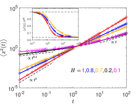
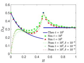
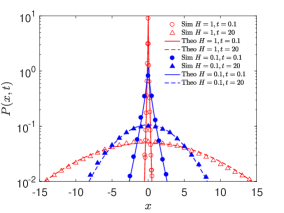
Figure 1: Dynamics of the FBM-DD model. Left: Comparison between simulations of equation (1) and the exact MSD (47) for $H=1$ as well as numerical integration of (4) for different $H$. The MSD approaches the limits (dashed lines) $t^{2H}$ at short times and, at long times, anomalous [$(2/\pi)t^{2H}$] or normal [$2D_{\mathrm{eff}}t$] scaling for super- and subdiffusion, respectively. Middle: Effective diffusion coefficient as function of $H$. The theoretical curve (equation (57) for $H<1/2$ and $1/\pi$ for $H>1/2$) shows a distinct discontinuity at the Brownian value $H=1/2$. Results from numerical evaluation of equations (48), (4), and simulations are shown to gradually approach the theoretical values (see text and D). Right: Crossover of the PDF from short-time non-Gaussian form with exponential tails to long-time Gaussian. The crossover is described in terms of the kurtosis (see text).

We first demonstrate how to get the main results for the MSD from simple estimates at short and long times compared to the correlation time of $D(t)$ dynamics. As the diffusion coefficient does not change considerably at times shorter than the correlation time, $K(0)\approx\langle\sqrt{D(t)D(t)}\rangle=\langle D\rangle=1/2$, equation (4) yields

$$\langle x^{2}(t)\rangle\sim 4\langle D\rangle\int_{0}^{t}(t-\tau)\langle\xi^{2}_{H}\rangle_{\tau}d\tau=t^{2H}.$$ (5)

For long times $t\gg 1$, more care is needed: as we will see, the long-time limit is different for the persistent and anti-persistent cases. For the persistent case $H>1/2$ we assume that the main contribution to the integral in equation (4) at long times comes from large $\tau$, since the noise autocorrelation decays very slowly. We thus approximate $K(\tau)\approx\langle|Y(t)|\rangle\langle|Y(t+\tau)|\rangle=\langle|Y(t)|\rangle^{2}=1/\pi$. Then,

$$\langle x^{2}(t)\rangle\sim 4\langle|Y(t)|\rangle^{2}\int_{0}^{t}(t-\tau)\langle\xi^{2}_{H}\rangle_{\tau}=(2/\pi)t^{2H}.$$ (6)

In the anti-persistent case $H<1/2$ we split equation (4) into two integrals, $4t\int_{0}^{t}K(\tau)\langle\xi^{2}_{H}\rangle_{\tau}d\tau$ and $-4\int_{0}^{t}\tau K(\tau)\langle\xi^{2}_{H}\rangle_{\tau}d\tau$. In the first integral at long times it is eligible to replace the upper limit of the integral by infinity, since it converges. The second integral produces a subleading term, since it is bounded from above by $Ct^{2H}$, $C$ being a constant. We therefore have the following asymptotic result for the MSD in the anti-persistent case at long times,

$$\langle x^{2}(t)\rangle\sim 2D_{\mathrm{eff}}t,$$ (7)

with $D_{\mathrm{eff}}=\lim_{\delta\to 0}2\int_{0}^{+\infty}K(\tau)\langle\xi^{2}_{H}\rangle_{\tau}d\tau$. Thus, the FBM-DD model demonstrates surprising crossovers in the behaviour of the MSD. In the persistent case the MSD scales as $t^{2H}$ at both short and long times, but with different diffusion coefficients. This is in a sharp contrast with the Brownian yet non-Gaussian diffusion characterised by the same, invariant diffusivity at all times. In the antipersistent case the situation is even more counterintuitive: the subdiffusive scaling of the MSD at short times crosses over to normal diffusion at long times.

The behaviour of the MSD is shown in figure 1. For superdiffusion, the change of the diffusivity between the short and long time superdiffusive scaling $\simeq t^{2H}$ is distinct. Excellent agreement is observed between the exact and numerical evaluation for $H=1$ and $H=0.7,0.8$, respectively. The exact analytical expression for $H=1$ is derived in C. In the subdiffusive case simulations and numerical evaluation nicely coincide and show the crossover from subdiffusion to normal diffusion. Figure 1 also shows the effective long time diffusivity. For superdiffusion the constant value $2/\pi\approx 0.63$ is distinct from the $H$-dependency for subdiffusion ($H<1/2$). For the Brownian case, $D_{\mathrm{eff}}=1/2$, leading to a distinct discontinuity at $H=1/2$. Note the slow convergence to the theory of simulations results and numerical evaluation of the respective integrals (see D for details).

Given the above arguments that at short times ($t\ll 1$) the diffusivity is approximately constant, we expect that in this regime the PDF corresponds to the superstatistical average of a single Gaussian over the stationary diffusivity distribution of the Ornstein-Uhlenbeck process,

$$P(x,t)=(\pi\langle x^{2}(t)\rangle_{\mathrm{ST}}^{1/2})^{-1}K_{0}(x/\langle x^{2}(t)\rangle_{\mathrm{ST}}^{1/2}),$$ (8)

where $\langle x^{2}(t)\rangle_{\mathrm{ST}}=t^{2H}$ and $K_{0}$ is the modified Bessel function of the second kind [6]. For long times ($t\gg 1$) the diffusivity correlations decay and the Gaussian limit $P(x,t)=G(\langle x^{2}(t)\rangle_{\mathrm{LT}})$ is recovered, where

$$G(\langle x^{2}(t)\rangle)=(2\pi\langle x^{2}(t)\rangle)^{-1/2}\exp\left(-x^{2}/[2\langle x^{2}(t)\rangle]\right).$$ (9)

For $H>1/2$, the long-time MSD is $\langle x^{2}(t)\rangle_{\mathrm{LT}}=(2/\pi)t^{2H}$ while for $H<1/2$, $\langle x^{2}(t)\rangle_{\mathrm{LT}}=2D_{\mathrm{eff}}t$. The crossover behaviour of $P(x,t)$ is indeed corroborated in figure 1 for different values of $H$.

How do these observations compare to generalisations of other established random-diffusivity models? While in the normal-diffusive regime these models encode very similar behaviour, we show now that striking differences in the dynamics emerge when the motion is governed by long-range correlations.

3 FBM-generalisation of the Tyagi-Cherayil (TC) model

The generalised TC model [11] in dimensionless units reads

$$dx/dt=\sqrt{2}Z(t)\xi_{H}(t),\,\,\,\,dZ/dt=-Z(t)+\eta(t).$$ (10)

This expression is obtained from the original equations (E) via the transformations $t\to t/\tau_{c}$ and $x\to x/(\sigma_{1}\sigma_{2}\tau_{c}^{H+1/2})$. Using the same notation as before, $\eta$ represents zero-mean white Gaussian noise and $\xi_{H}(t)$ is fractional Gaussian noise with Hurst exponent $H$.

The TC model looks quite similar to the minimal DD model, however, there exists a decisive difference: In equations (10) the OU-process $Z(t)$ enters without the absolute value used in the minimal DD model (1). In expression (10) the prefactor $Z(t)$ is therefore not a diffusion coefficient (by definition, a non-negative quantity). In the case $H=1/2$, the noise $\xi_{1/2}(t)$ is white, that is, uncorrelated, and has zero mean. Due to the symmetry of the OU-process (for symmetric initial condition) and the noise $\xi_{1/2}(t)$, the absolute value of $Z(t)$ can be treated as the diffusion coefficient. In the fractional case, we may still treat $|Z(T)|$ as a diffusion coefficient, however, in the correlated (persistent or antipersistent) cases we would then imply a compulsory change in the sign of $\xi(t)$ when $Z(t)$ changes sign. Yet this model is principally different from the formulation in (10). As our discussion shows, the close similarity between the TS and DD models in the case $H=1/2$ is replaced by a distinct dissimilarity in the emerging dynamics.

The MSD of the FBM-TC model reads

$$\langle x^{2}(t)\rangle=4\int_{0}^{t}(t-\tau)K(\tau)\langle\xi^{2}_{H}\rangle_{\tau}d\tau,$$ (11)

where the kernel $K(\tau)$ is defined as

$$K(\tau)=\langle Z(t_{1})Z(t_{2})\rangle=\exp(-\tau)/2.$$ (12)

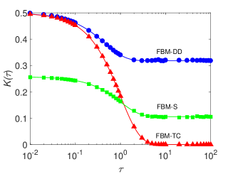
Figure 4: Comparison between simulations of the respective stochastic equations (circles, triangles, and squares) and the exact autocorrelation function $K(\tau)$ (solid curves) of the three diffusing-diffusivity models: FBM-DD (blue, equation (31)), FBM-TC (red, equation (12)), and FBM-S (green, equation (82)). The parameters of the FBM-S model are $D_{1}=1$, $D_{2}=0.01$, $k_{12}=3/4$, and $k_{21}=1/4$.

It is shown in figure 4 along with the corresponding Langevin simulations.

Before presenting the exact solution, let us apply an analogous reasoning for the behaviour of the MSD as developed for the FBM-DD model above. Namely, at short times we approximate $K(\tau)\approx\langle Z^{2}\rangle=1/2$. Then equation (11) becomes $\langle x^{2}(t)\rangle\approx 4\langle D\rangle\int_{0}^{t}(t-\tau)\langle\xi_{H}^{2}\rangle_{\tau}d\tau\propto t^{2H}$. At long times the MSD can be composed of the two parts $\langle x^{2}(t)\rangle=4t\int_{0}^{t}K(\tau)\langle\xi_{H}^{2}\rangle_{\tau}d\tau-4\int_{0}^{t}\tau K(\tau)\langle\xi_{H}^{2}\rangle_{\tau}d\tau$. The upper limit of the first integral can be replaced by infinity because the first integral converges in both persistent and anti-persistent cases at long times ($K(\tau)$ decays to 0 exponentially, different from the FBM-DD model). The second term is subleading in comparison to the first term. As a result the MSD at long times scales linearly in time, $\langle x^{2}(t)\rangle\sim 2D_{\mathrm{eff}}t$, for both sub- and superdiffusion, where $D_{\mathrm{eff}}=\lim_{\delta\to 0}2\int_{0}^{\infty}K(\tau)\langle\xi_{H}^{2}\rangle_{\tau}d\tau$.

Indeed, from the exact form of the MSD in E we obtain the limiting behaviours

$$\langle x^{2}(t)\rangle\sim\left\{\begin{array}[]{ll}t^{2H},&t\to 0\\ \Gamma(2H+1)t,&t\to\infty\end{array}\right..$$ (13)

Thus for both sub- and superdiffusion this model shows a crossover from anomalous to normal diffusion, as demonstrated in figure 2. The effective long-time diffusion coefficient in this model varies continuously as $D_{\mathrm{eff}}=\Gamma(2H+1)/2$ for all $H$. In particular, this means that for $H=1/2$, $D_{\mathrm{eff}}=1/2$. Figure 2 shows the exact match of the simulations results and the numerical evaluation at finite integration step.

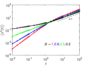
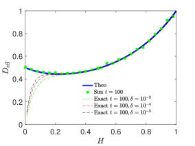
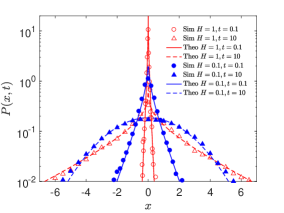
Figure 2: Dynamics of the FBM-TC model. Left: Crossover dynamics of the MSD, showing simulations (symbols) and the solution (67). For both sub- and superdiffusion the long-time scaling is Brownian. Middle: Continuous variation of the effective diffusion coefficient with $H$. The exact result (71) gradually converges to the theoretical curve for different $\delta$ and $t$. Right: Crossover of the PDF from short-time non-Gaussian shape with exponential tails to a long-time Gaussian. The crossover is described in terms of the kurtosis in E.

The PDF at short times coincides with the superstatistical limit in expression (8) above, as shown explicitly in equation (72). At long times we recover the Gaussian $P(x,t)=G(\Gamma(2H+1)t)$. Note that for $H=1$ the noise is equal to unity at all times and the dynamics of $x(t)$ is completely determined by the superstatistic encoded by the OU-process $Z(t)$. The tails of the PDF are thus always exponential, reflected by the fact that the kurtosis has the invariant value 9 (see E).

Despite the strong similarity between the DD and TC models in the Brownian case, for correlated driving noise their detailed behaviour is strikingly dissimilar, due to the different asymptotic forms of the kernel $K(\tau)$ (figure 4).

4 FBM-generalisation of the Switching (S) model

The third case model we consider here is the S-model with generalised noise [14],

$$dx/dt=\sqrt{2}\theta(t)\xi_{H}(t),\,\,\,\,\theta(t)=[D_{2}^{1/2}-D_{1}^{1/2}]n(t)+D_{1}^{1/2},$$ (14)

where $n(t)$ is a two-state Markov chain switching between the values $\{0,1\}$ and $\xi_{H}(t)$ represents again fractional Gaussian noise. The constants $D_{i}$ are the diffusivities in the two states. The switching rates are $k_{12}$ and $k_{21}$, such that the correlation time is $\tau_{c}=1/(k_{12}+k_{21})$.

From the first and second moments of the process $\theta(t)$, equations (81) and (82), we calculate the MSD of the process. In the Brownian limit $H=1/2$ the MSD has a linear dependence at all times,

$$\langle x^{2}(t)\rangle=2(k_{21}D_{1}+k_{12}D_{2})\tau_{c}t.$$ (15)

This result was also obtained in [15]. For the general case with the correlation function based on fractional Gaussian noise, we have

$$\langle x^{2}(t)\rangle = 4\int_{0}^{t}(t-\tau)K(\tau)\langle\xi^{2}_{H}\rangle_{\tau}d\tau$$ (16)

$$= 2a_{1}e^{-t/\tau_{c}}t^{2H}+2a_{2}t^{2H}+4Ha_{1}\tau_{c}^{2H-1}\gamma(2H,t/\tau_{c})t$$

$$+2(1-2H)a_{1}\tau_{c}^{2H}\gamma(2H+1,t/\tau_{c})$$

$$-\frac{2a_{1}(t+1)\delta^{2H}}{(H+1)(2H+1)}-\frac{2a_{2}\delta^{2H}}{(H+1)(2H+1)}+o(\delta^{2H}),$$

where $K(\tau)=\left\langle\theta(t_{1})\theta(t_{2})\right\rangle$, $a_{1}=(D_{2}^{1/2}-D_{1}^{1/2})^{2}k_{12}k_{21}\tau_{c}^{2}$, and $a_{2}=(k_{21}D_{1}^{1/2}+k_{12}D_{2}^{1/2})^{2}\tau_{c}^{2}$. At short times $t\ll\tau_{c}$ we find the scaling behaviour

$$\langle x^{2}(t)\rangle_{\mathrm{ST}}\sim 2(a_{1}+a_{2})t^{2H}=2(k_{21}D_{1}+k_{12}D_{2})\tau_{c}t^{2H}.$$ (17)

At long times $t\gg\tau_{c}$ the same scaling law is obtained, but with a different prefactor for the persistent case ($H>1/2$),

$$\left\langle x^{2}(t)\right\rangle_{\mathrm{LT}}\sim 2a_{2}t^{2H}=2[k_{21}D_{1}^{1/2}+k_{12}D_{2}^{1/2}]^{2}\tau_{c}^{2}t^{2H}.$$ (18)

In contrast, for the anti-persistent case ($H<1/2$), we derive a crossover to normal diffusion,

$$\left\langle x^{2}(t)\right\rangle_{\mathrm{LT}}\simeq 2D_{\mathrm{eff}}t\langle x^{2}(t)\rangle\sim 2[\Gamma(2H+1)\tau^{2H-1}a_{1}]t.$$ (19)

From equations (15), (18), and (19), the long-time effective diffusivity can be obtained as

$$D_{\mathrm{eff}}=\left\{\begin{array}[]{ll}(k_{21}D_{1}^{1/2}+k_{12}D_{2}^{1/2})^{2}\tau_{c}^{2},&1/2<H\leq 1\\[5.69046pt] (k_{21}D_{1}+k_{12}D_{2})\tau_{c},&H=1/2\\[5.69046pt] \Gamma(2H+1)(D_{2}^{1/2}-D_{1}^{1/2})^{2}k_{12}k_{21}\tau_{c}^{2H+1},&0<H<1/2\end{array}\right..$$ (23)

The crossover behaviours of the MSD in the peristent and anti-persistent cases, analogous to the difference in the long-time scalings of the FBM-DD model, are displayed in figure 3. We also see some similarities between the FBM-S and FBM-DD models for the effective diffusivity. For the TC-DD model an $H$-dependent behaviour for $H<1/2$ is followed by a discontinuity at $H=1/2$ and then a constant value for $H>1/2$. The results of the MSD for finite values $\delta$ and $t$ are given in F.

Next we discuss the PDF and kurtosis. At short times the continuous superstatistic of the previous cases is reduced to the discrete case of two superimposed Gaussians, producing the non-exponential form

$$P(x,t) = P(x,t|\theta(t)=D_{1}^{1/2})\times\mathrm{Pr}\{\theta(t)=D_{1}^{1/2}\}$$ (24)

$$+P(x,t|\theta(t)=D_{2}^{1/2})\times\mathrm{Pr}\{\theta(t)=D_{2}^{1/2}\}$$

$$= [k_{21}G(2D_{1}t^{2H})+k_{12}G(2D_{2}t^{2H})]\tau_{c}.$$

At long times a single Gaussian dominates,

$$P(x,t)\sim G\left(\langle x^{2}(t)\rangle_{\mathrm{LT}}\right),$$ (25)

where $\langle x^{2}(t)\rangle_{\mathrm{LT}}$ is given by equations (18) and (19) for the super- and subdiffusive cases, respectively. Figure 3 shows the superimposed two Gaussians at short times and the single Gaussian at long times.

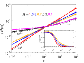
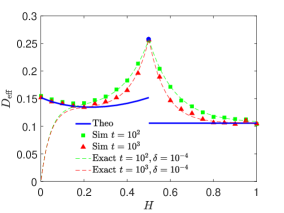
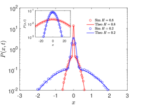
Figure 3: Dynamics of the FBM-S model. Left: crossover dynamics of the MSD showing simulations (symbols) and result (16). For sub- and superdiffusion, respectively, the long-time scaling is $t^{2H}$ and $2D_{\mathrm{eff}}t$. Middle: $D_{\mathrm{eff}}$ as function of $H$. The theoretical behaviour (23) shows a distinct discontinuity around the Brownian case $H=1/2$. The gradual convergence of simulations and results (83) and (84) for different $t$ and $\delta$ are shown. Right: Initially the non-Gaussian shape is composed of two Gaussians with different diffusivity. At long times a single Gaussian emerges. The crossover is described in terms of the kurtosis (see F).

5 Conclusions

Viscoelastic anomalous diffusion with long-ranged correlations is a non-Markovian, natively Gaussian process widely observed in complex liquids and the cytoplasm of biological cells. Most data analyses have concentrated on the MSD and the displacement autocorrelation function. Yet, once probed, the PDF in many of these systems turns out to be non-Gaussian, a phenomenon ascribed to the heterogeneity of the systems. Building on recent results for Brownian yet non-Gaussian diffusion, in which the non-Gaussian ensemble behaviour is understood as a consequence of a heterogeneous diffusivity coefficient, we here analysed three different random-diffusivity models driven by correlated Gaussian noise.

Despite the simplicity of these models we observed surprising behaviours. Thus, while in the Brownian case all models display a linear PSD with invariant diffusion coefficient, in the correlated case a crossover occurs from short to long-time behaviours, with respect to the intrinsic correlation times. In particular, whether the long-time scaling of the MSD is anomalous or normal, depends on the specific model. Moreover, the effective diffusivity exhibits unexpectedly complex behaviours with discontinuities in the FBM-DD and FBM-S models.

In all cases a crossover from an initial non-Gaussian to a Gaussian PDF occurs. We showed that the FBM-S model is different from the other models in that it encodes an initial superposition of two Gaussians, turning into a single Gaussian at long times. We note that while the short-time exponential shape may point towards a universal, extreme-value jump-dominated dynamics [16], data also show stretched-Gaussian shapes [34], as well as long(er)-time convergence towards an exponential [7]. Clearly, the phenomenology of heterogeneous environments is rich and needs further investigation.

Experimentally, the behaviours unveiled here may be used to explore further the relevance of the different possible stochastic formulations of random-diffusivity processes. For instance, in artificially crowded media one may vary the Hurst exponent by changing the volume fraction of crowders or the tracer sizes, or add drugs to change the system from super- to subdiffusive [25]. Comparison of the resulting scaling behaviours of MSD and associated effective diffusivity may then yield decisive clues.

The results found here will also be of interest in mathematical finance. In fact, the original DD model is equivalent to the Heston model [45] used to describe return dynamics of financial markets. Fractional Gaussian noise in mathematical finance is used to include an increased "roughness" to the emerging dynamics [46]. The different models studied here could thus enrich market models.

The CLT is a central dogma in statistical physics, based on the fact that the entry variables are identically distributed. For inhomogeneous environments, ubiquitous in many complex systems, new concepts generalising the CLT will have to be developed. While random-diffusivity models are a start in this direction and provide relevant strategies for data analyses [47], ultimately more fundamental models including the quenched nature of the disordered environment [18] need to be conceived.

Appendix A Dimensionless units for the FBM-DD model

In dimensional form the starting equations governing the evolution of the position $x(t)$ of the diffusing particle in the fractional version of the minimal DD-model read

$$\frac{d}{dt}x(t)=\sqrt{2D(t)}\sigma_{1}\xi_{H}(t),\,\,\,D(t)=Y^{2}(t),\,\,\,\frac{d}{dt}Y(t)=-\frac{Y}{\tau_{c}}+\sigma_{2}\eta(t).$$ (26)

Here $D(t)$ is the diffusion coefficient of dimension $[D]=\mathrm{cm}^{2}/\mathrm{sec}$, $\xi_{H}$ represents fractional Gaussian noise with the Hurst index $H\in(0,1]$ whose dimension is $[\xi_{H}]=\mathrm{sec}^{H-1}$ and whose correlation function reads [30]

$$\langle\xi_{H}(t)\xi_{H}(t+\tau)\rangle\equiv\langle\xi^{2}_{H}\rangle_{\tau}=(2\delta^{2})^{-1}\left((\tau+\delta)^{2H}-2\tau^{2H}+|\tau-\delta|^{2H}\right).$$ (27)

Moreover, $\sigma_{1}$ in equation (26) is the noise amplitude of dimension $[\sigma_{1}]=\mathrm{sec}^{1/2-H}$. $Y(t)$ is an auxiliary Ornstein-Uhlenbeck process with correlation time $\tau_{c}$, $\eta(t)$ is a white Gaussian noise with zero mean and unit variance. $\sigma_{2}$ of units $[\sigma_{2}]=\mathrm{cm}/\mathrm{sec}$ is the noise amplitude associated with $\eta(t)$. To simplify the calculations and to obtain a more elegant formulation we introduce dimensionless variables according to $t^{\prime}=t/t_{0}$ and $x^{\prime}=x/x_{0}$. Equations (26) then become

$$\frac{dx^{\prime}}{dt^{\prime}}=\sqrt{2D(t_{0}t^{\prime})}\frac{t_{0}\sigma_{1}}{x_{0}}\xi_{H}(t_{0}t^{\prime}),\,\,\,D(t_{0}t^{\prime})=Y^{2}(t_{0}t^{\prime}),\,\,\,\frac{dY}{dt^{\prime}}=-\frac{Y}{\tau_{c}/t_{0}}+\sigma_{2}t_{0}\eta(t_{0}t^{\prime}).$$

Noting that for the Gaussian noise sources we have $\xi_{H}(t_{0}t^{\prime})=t_{0}^{H-1}\xi_{H}(t^{\prime})$ and $\eta(t_{0}t^{\prime})=t_{0}^{-1/2}\eta(t^{\prime})$ we rewrite equations (26) as

$$\frac{dx^{\prime}}{dt^{\prime}}=\sqrt{2\overline{D}(t^{\prime})}\xi_{H}(t^{\prime}),\,\,\,\overline{D}(t^{\prime})=\overline{Y}^{2}(t^{\prime}),\,\,\,\frac{d\overline{Y}}{dt^{\prime}}=-\frac{\overline{Y}}{\overline{\tau}_{c}}+\overline{\sigma}_{2}\eta(t^{\prime}),$$

where

$$\overline{D}=\frac{\sigma_{1}^{2}t_{0}^{2H}}{x_{0}^{2}}D,\quad\overline{Y}=\frac{\sigma_{1}t_{0}^{H}}{x_{0}}Y,\quad\overline{\tau}_{c}=\frac{\tau_{c}}{t_{0}},\quad\overline{\sigma_{2}}=\frac{\sigma_{1}t_{0}^{1/2+H}}{x_{0}}\sigma_{2}.$$

Now, we choose the temporal and spatial scales such that $\overline{\tau}_{c}=\overline{\sigma}_{2}=1$, such that

$$t_{0}=\tau_{c},\quad x_{0}=\sigma_{1}\sigma_{2}\tau_{c}^{1/2+H}.$$

With this choice of units, the stochastic equations of our minimal FBM-DD model are then given by equation (1) and (2) of the main text.

Appendix B Calculation of the integral kernel $K(\tau)$

Introducing $a(\tau)=e^{-\tau}$ and $b(\tau)=\sqrt{1-a^{2}(\tau)}$ we write $K(\tau)$ in equation (4) of the main text as

$$K(\tau) = \langle|Y(t_{1})||Y(t_{2})|\rangle_{\tau=|t_{2}-t_{1}|}$$ (28)

$$= \int_{-\infty}^{\infty}dY_{1}\int_{-\infty}^{\infty}dY_{2}|Y_{1}||Y_{2}|\frac{\exp\left(-[Y_{1}^{2}-2aY_{1}Y_{2}+Y_{2}^{2}]/b^{2}\right)}{\pi b}$$

$$= \frac{2}{\pi b}\int_{0}^{\infty}dY_{1}\int_{0}^{\infty}dY_{2}Y_{1}Y_{2}\exp\left(-\frac{Y_{1}^{2}-2aY_{1}Y_{2}+Y_{2}^{2}}{b^{2}}\right)$$

$$+\frac{2}{\pi b}\int_{0}^{\infty}dY_{1}\int_{0}^{\infty}dY_{2}Y_{1}Y_{2}\exp\left(-\frac{Y_{1}^{2}+2aY_{1}Y_{2}+Y_{2}^{2}}{b^{2}}\right)$$

$$= \frac{b}{\pi}\int_{0}^{\infty}dY_{1}\frac{\partial}{\partial a}\left[\int_{0}^{\infty}dY_{2}\exp\left(-\frac{Y_{1}^{2}+Y_{2}^{2}}{b^{2}}+\frac{2a}{b^{2}}Y_{1}Y_{2}\right)\right]$$

$$-\frac{b}{\pi}\int_{0}^{\infty}dY_{1}\frac{\partial}{\partial a}\left[\int_{0}^{\infty}dY_{2}\exp\left(-\frac{Y_{1}^{2}+Y_{2}^{2}}{b^{2}}-\frac{2a}{b^{2}}Y_{1}Y_{2}\right)\right]$$

$$= B_{1}-B_{2}.$$

Using the integral

$$\int_{0}^{\infty}\exp\left(-px^{2}-qx\right)dx=\frac{1}{2}\sqrt{\frac{\pi}{p}}\exp\left(\frac{q^{2}}{4p}\right)\mathrm{erfc}\left(\frac{q}{2\sqrt{p}}\right),$$

where $\mathrm{erfc}(z)=1-\mathrm{erf}(z)=2\pi^{-1/2}\int_{z}^{+\infty}e^{-t^{2}}dt$ is the complementary error function, we rewrite $B_{1}$ and $B_{2}$ as

$$B_{1} = \frac{b}{\pi}\int_{0}^{\infty}dY_{1}\exp\left(-\frac{Y_{1}^{2}}{b^{2}}\right)\frac{\partial}{\partial a}\left[\frac{\sqrt{\pi}b}{2}\exp\left(\frac{a^{2}Y_{1}^{2}}{b^{2}}\right)\mathrm{erfc}\left(-\frac{a}{b}Y_{1}\right)\right]$$ (29)

$$= \frac{b^{2}}{2\sqrt{\pi}}\int_{0}^{\infty}dY_{1}\exp\left(-\frac{Y_{1}^{2}}{b^{2}}\right)\frac{\partial}{\partial a}\left[\exp\left(\frac{a^{2}Y_{1}^{2}}{b^{2}}\right)\bigg{(}1+\mathrm{erf}\left(\frac{a}{b}Y_{1}\right)\bigg{)}\right],$$

and

$$B_{2} = \frac{b}{\pi}\int_{0}^{\infty}dY_{1}\exp\left(-\frac{Y_{1}^{2}}{b^{2}}\right)\frac{\partial}{\partial a}\left[\frac{\sqrt{\pi}b}{2}\exp\left(\frac{a^{2}Y_{1}^{2}}{b^{2}}\right)\mathrm{erfc}\left(\frac{a}{b}Y_{1}\right)\right]$$ (30)

$$= \frac{b^{2}}{2\sqrt{\pi}}\int_{0}^{\infty}dY_{1}\exp\left(-\frac{Y_{1}^{2}}{b^{2}}\right)\frac{\partial}{\partial a}\left[\exp\left(\frac{a^{2}Y_{1}^{2}}{b^{2}}\right)\bigg{(}1-\mathrm{\mathrm{erf}}\left(\frac{a}{b}Y_{1}\right)\bigg{)}\right].$$

Plugging equations (29) and (30) into (28) and after some transformations, we get

$$K(\tau) = \frac{b^{2}}{\sqrt{\pi}}\int_{0}^{\infty}dY\exp\left(-\frac{Y^{2}}{b^{2}}\right)\frac{\partial}{\partial a}\left[\exp\left(\frac{a^{2}Y^{2}}{b^{2}}\right)\mathrm{erf}\left(\frac{a}{b}Y\right)\right]$$ (31)

$$= \frac{2a}{\sqrt{\pi}}\int_{0}^{\infty}dYY^{2}e^{-Y^{2}}\mathrm{erf}\left(\frac{a}{b}Y\right)+\frac{2b}{\pi}\int_{0}^{\infty}dYY\exp\left(-\frac{Y^{2}}{b^{2}}\right)$$

$$= \frac{1}{\pi}\left[b(\tau)+a(\tau)\arctan\left(\frac{a(\tau)}{b(\tau)}\right)\right],$$

which is equation (4) in the main text. This result is verified by simulation of the Ornstein-Uhlenbeck process in figure S1. We immediately obtain the first-order and second-order derivatives of $K(\tau)$ with respect to $\tau$,

$$K^{\prime}(\tau)=-\frac{1}{\pi}a(\tau)\arctan\left(\frac{a(\tau)}{b(\tau)}\right),$$ (32)

and

$$K^{\prime\prime}(\tau)=\frac{1}{\pi}a(\tau)\left[\arctan\left(\frac{a(\tau)}{b(\tau)}\right)+\frac{a(\tau)}{b(\tau)}\right].$$ (33)

$K(\tau)$, $K^{\prime}(\tau)$ and $K^{\prime\prime}(\tau)$ are all monotonic and have the following limits

$$\lim\limits_{\tau\to 0}K(\tau)=\frac{1}{2},\quad\lim\limits_{\tau\to+\infty}K(\tau)=\frac{1}{\pi},$$

$$\lim\limits_{\tau\to 0}K^{\prime}(\tau)=-\frac{1}{2},\quad\lim\limits_{\tau\to+\infty}K^{\prime}(\tau)=0,$$

$$\lim\limits_{\tau\to 0}K^{\prime\prime}(\tau)=+\infty,\quad\lim\limits_{\tau\to+\infty}K^{\prime\prime}(\tau)=0.$$ (34)

Appendix C Exact MSD for $H=1$ in the FBM-DD model

Here we derive the formula for the MSD of the FBM-DD model in the fully persistent limit $H=1$. To this end we use equation (4) of the main text and thus $\langle\xi_{H}^{2}\rangle=1$. As result we get

$$\langle x^{2}(t)\rangle=\frac{4}{\pi}\int_{0}^{t}d\tau(t-\tau)\left[b(\tau)+a(\tau)\arctan\left(\frac{a(\tau)}{b(\tau)}\right)\right]=\frac{4}{\pi}(tI_{1}-I_{2}),$$ (35)

where

$$I_{1}=\int_{0}^{t}d\tau\left[b(\tau)+a(\tau)\arctan\left(\frac{a(\tau)}{b(\tau)}\right)\right]$$ (36)

and

$$I_{2}=\int_{0}^{t}d\tau\tau\left[b(\tau)+a(\tau)\arctan\left(\frac{a(\tau)}{b(\tau)}\right)\right].$$ (37)

We first concentrate on $I_{1}$. Introducing the new variable $\varphi$ such that $a(\tau)=\exp(-\tau)=\sin\varphi$ and $b(\tau)=\cos\varphi$, we see that $\tau=0$ corresponds to $\varphi=\pi/2$, while $\tau=\infty$ corresponds to $\varphi=0$. With $d\tau=-\cos\varphi d\varphi/\sin\varphi$ we find

$$I_{1}=\int_{\varphi_{t}}^{\pi/2}d\varphi\frac{\cos\varphi}{\sin\varphi}\left[\cos\varphi+\sin\varphi\arctan\left(\tan\varphi\right)\right]=\int_{\varphi_{t}}^{\pi/2}d\varphi\left[\frac{\cos^{2}\varphi}{\sin\varphi}+\varphi\cos\varphi\right],$$ (38)

where $\varphi_{t}=\arcsin(\exp(-\tau))$ with $\varphi_{t}\in(0,\pi/2)$. By using formula 1.5.6.15 from [48] we finally obtain

$$I_{1}=\frac{\pi}{2}-2\cos\varphi_{t}-\ln\left(\tan\frac{\varphi_{t}}{2}\right)-\varphi_{t}\sin\varphi_{t}.$$ (39)

Now we turn to the integral $I_{2}$ in equation (37). Introducing the indefinite integral

$$F(\tau) = \int d\tau\left[b(\tau)+a(\tau)\arctan\left(\frac{a(\tau)}{b(\tau)}\right)\right]$$

$$= \int d\varphi\left[\frac{\cos^{2}\varphi}{\sin\varphi}+\varphi\cos\varphi\right]$$

$$= -2\cos\varphi-\ln\left|\mathrm{tan}\frac{\varphi}{2}\right|-\varphi\sin\varphi$$

and integrating $I_{2}$ by parts yields

$$I_{2}=\tau F(\tau)\Big{|}_{\tau=0}^{\tau=t}-\int_{0}^{t}F(\tau)d\tau=-t\Bigg{(}2\cos\varphi_{t}+\ln\left(\tan\frac{\varphi_{t}}{2}\right)+\varphi_{t}\sin\varphi_{t}\Bigg{)}+I_{21}+I_{22}+I_{23},$$ (40)

where

$$I_{21}=2\int_{\varphi_{t}}^{\pi/2}\frac{\cos^{2}\varphi}{\sin\varphi}=-2\cos\varphi_{t}-2\ln\left(\tan\frac{\varphi_{t}}{2}\right),$$ (41)

$$I_{22}=\int_{\varphi_{t}}^{\pi/2}\varphi\cos\varphi d\varphi=\frac{\pi}{2}-\cos\varphi_{t}-\varphi_{t}\sin\varphi_{t},$$ (42)

and

$$I_{23}=\int_{\varphi_{t}}^{\pi/2}d\varphi\frac{\cos\varphi}{\sin\varphi}\ln\left(\tan\frac{\varphi}{2}\right).$$ (43)

Introducing the new variables $y=\tan\frac{\varphi}{2}$ and $z=\tan^{2}\frac{\varphi}{2}$, our integral $I_{23}$ becomes

$$I_{23} = \int_{\tan\left(\varphi_{t}/2\right)}^{1}\frac{1-y^{2}}{(1+y^{2})y}\ln ydy=\int_{\tan\left(\varphi_{t}/2\right)}^{1}\frac{\ln y}{y}dy-\int_{\tan(\varphi_{t}/2)}^{1}\frac{2y\ln y}{1+y^{2}}dy$$ (44)

$$= -\frac{1}{2}\ln^{2}\left(\tan\frac{\varphi_{t}}{2}\right)-\frac{1}{2}\int_{\tan^{2}(\varphi_{t}/2}^{1}\frac{\ln z}{1+z}dz.$$

Taking into account formula 1.6.3.8 from [48] for the indefinite integral,

$$\int\frac{\ln x}{x+a}dx=\ln x\ln\frac{x+a}{a}+\mathrm{Li}_{2}(-\frac{x}{a}),$$

where the polylogarithm is defined as

$$\mathrm{Li}_{s}(z)=\sum_{k=1}^{\infty}\frac{z^{k}}{k^{s}},\quad|z|<1.$$

For the integral $I_{23}$ in equation (42) we obtain

$$I_{23} = -\frac{1}{2}\mathrm{Li}_{2}(-1)-\frac{1}{2}\ln^{2}\left(\tan\frac{\varphi_{t}}{2}\right)+\ln\left(\tan\frac{\varphi_{t}}{2}\right)\ln\left(1+\tan^{2}\frac{\varphi_{t}}{2}\right)$$ (45)

$$+\frac{1}{2}\mathrm{Li}_{2}\left(-\tan^{2}\frac{\varphi_{t}}{2}\right).$$

After replacing $\mathrm{Li}_{2}(-1)=-\pi^{2}/12$ and plugging equations (41), (42), and (45) into (40) we get

$$I_{2}= - t\left(2\cos\varphi_{t}+\ln\left(\tan\frac{\varphi_{t}}{2}\right)+\varphi_{t}\sin\varphi_{t}\right)-3\cos\varphi_{t}-2\ln\left(\tan\frac{\varphi_{t}}{2}\right)+\frac{\pi}{2}-\varphi_{t}\sin\varphi_{t}$$ (46)

$$+ \frac{\pi^{2}}{24}-\frac{1}{2}\ln^{2}\left(\tan\frac{\varphi_{t}}{2}\right)+\ln\left(\tan\frac{\varphi_{t}}{2}\right)\ln\left(1+\tan^{2}\frac{\varphi_{t}}{2}\right)+\frac{1}{2}\mathrm{Li}_{2}\left(-\tan^{2}\frac{\varphi_{t}}{2}\right).$$

Now, with $\varphi_{t}=\arcsin(\exp(-t))=\arcsin a(t)$, $\varphi_{t}\in(0,\pi/2)$, $\cos\varphi_{t}=b(t)$, and $\tan(\varphi_{t}/2)=\sin\varphi_{t}/(1+\cos\varphi_{t})=a(t)/(1+b(t))$, equation (46) along with (39) yields the MSD, equation (35) in the form

$$\langle x^{2}(t)\rangle = \frac{2}{\pi}\Bigg{[}t^{2}+(\pi-4+2\ln 2)t+6b(t)+2a(t)\arctan\left(\frac{a(t)}{b(t)}\right)-\ln^{2}\big{(}1+b(t)\big{)}$$ (47)

$$+ 2(\ln 2-2)\ln\big{(}1+b(t)\big{)}-\mathrm{Li}_{2}\left(-\frac{1-b(t)}{1+b(t)}\right)-\pi(1+\frac{\pi}{12})\Bigg{]}.$$

Appendix D Effective long time diffusivity $D_{\mathrm{eff}}$ for $H\in(0,1/2]$ in the FBM-DD model

Consider the integral

$$W(0,t,\delta)=2\int_{0}^{t}K(\tau)\left\langle\xi_{H}^{2}\right\rangle_{\tau}d\tau$$ (48)

with $t\gg 1\gg\delta$. Then the effective long-time diffusivity of the main text, equation (7), reads

$$D_{\mathrm{eff}}(H\leq 1/2)=\lim\limits_{\delta\to 0,t\to\infty}W(0,t,\delta).$$ (49)

For $H=1/2$ the correlation function $\langle\xi_{H}^{2}\rangle_{\tau}$ is reduced to a piece-wise function, and the efficient diffusivity becomes

$$D_{\mathrm{eff}}(H=1/2)=\lim\limits_{\delta\to 0}2\int_{0}^{\delta}K(\tau)\frac{\delta-\tau}{\delta^{2}}d\tau=\lim\limits_{\delta\to 0}\int_{0}^{\delta}(1-\tau)\frac{\delta-\tau}{\delta^{2}}d\tau=\frac{1}{2},$$ (50)

where we approximate $K(\tau)$ in equation (31) by the first-order term when $\tau\ll 1$, i.e., $K(\tau)=(1-\tau)/2+o(\tau)$.

Next we consider the efficient diffusivity for $H\in(0,1/2)$. Introducing the short-time scale $\Delta$, which satisfies

$$\delta\ll\Delta\ll 1,$$ (51)

we split equation (48) into two parts,

$$W(0,t,\delta)=W(0,\Delta,\delta)+W(\Delta,t,\delta).$$ (52)

Noting that the integral variable satisfies $\tau\leq\Delta\ll 1$ in the first part, we use the first-order approximate $K(\tau)=(1-\tau)/2+o(\tau)$, such that

$$W(0,\Delta,\delta)=H\Delta^{2H-1}-(H-\frac{1}{2})\Delta^{2H}-\frac{\delta^{2H}}{(2H+1)(2H+2)}+o(\delta^{2H}).$$ (53)

In the second part the integral variable satisfies $\tau\geq\Delta\gg\delta$, and we use $\langle\xi_{H}^{2}\rangle_{\tau}=H(2H-1)\tau^{2H-2}$, yielding

$$W(\Delta,t,\delta) = 2HK(\tau)\tau^{2H-1}\Big{|}^{t}_{\Delta}-K^{\prime}(\tau)\tau^{2H}\Big{|}^{t}_{\Delta}+\int_{\Delta}^{t}\tau^{2H}K^{\prime}(\tau)d\tau$$ (54)

$$= \frac{2H}{\pi}t^{2H-1}-H(1-\Delta)\Delta^{2H-1}+K^{\prime}(\Delta)\Delta^{2H}$$

$$+\int_{\Delta}^{t}\tau^{2H}K^{\prime\prime}(\tau)d\tau+o(\Delta^{2H}),$$

where $K(\Delta)=(1-\Delta)/2+o(\Delta)$ and $K^{\prime}(t)\sim\exp(-t)$ for $t\gg 1$. After plugging equations (53) and (54) into (52), we have

$$W(0,t,\delta) = (\frac{1}{2}+K^{\prime}(\Delta))\Delta^{2H}+\int_{\Delta}^{t}\tau^{2H}K^{\prime\prime}(\tau)d\tau-\frac{\delta^{2H}}{(2H+1)(2H+2)}$$ (55)

$$+\frac{2H}{\pi}t^{2H-1}+o(\Delta^{2H})+o(\delta^{2H}).$$

From the properties of $K(\tau)$ in equation (34), $\lim\limits_{\tau\to 0}K^{\prime\prime}(\tau)\sim\tau^{-1/2}$ and thus $\lim\limits_{\Delta\to 0}\int_{\Delta}^{t}\tau^{2H}K^{\prime\prime}(\tau)d\tau$ converges. We then have

$$W(0,t,\delta)\sim\int_{0}^{t}\tau^{2H}K^{\prime\prime}(\tau)d\tau-\frac{\delta^{2H}}{(2H+1)(2H+2)}+\frac{2H}{\pi}t^{2H-1}.$$ (56)

Considering the definition of the effective diffusivity, equation (49), and combining with the case $H=1/2$ we get

$$D_{\mathrm{eff}}(H\leq 1/2)=\left\{\begin{array}[]{ll}\int_{0}^{\infty}\tau^{2H}K^{\prime\prime}(\tau)d\tau,&0<H<1/2\\[5.69046pt] 1/2,&H=1/2\\ \end{array}\right..$$ (57)

The long-time effective diffusivity approaches $1/2$ when $H\to 0$ as $\lim\limits_{H\to 0}\int_{0}^{\infty}K^{\prime\prime}(\tau)d\tau=1/2$ and is discontinuous at $H=1/2$ because $\lim\limits_{H\to 1/2}\int_{0}^{\infty}\tau^{2H}K^{\prime\prime}(\tau)d\tau=1/2-1/\pi$.

Appendix E FBM-generalisation of the Tyagi-Cherayil model

We now consider the fractional Tyagi-Cherayil (TC) model

$$\frac{dx}{dt} = \sqrt{2}Z(t)\sigma_{1}\xi_{H}(t),$$ (58)

$$\frac{dZ}{dt} = -\frac{Z(t)}{\tau_{c}}+\sigma_{2}\eta(t).$$ (59)

Here $\xi_{H}(t)$ represents fractional Gaussian noise, $\eta(t)$ is a white Gaussian noise, and the respective correlation functions are the same as in equation (26). $Z(t)$ has dimension $[Z(t)]=\mathrm{cm}/\mathrm{sec}^{1/2}$ and $[\sigma_{1}]=\mathrm{sec}^{1/2-H}$, $[\sigma_{2}]=\mathrm{cm}/\mathrm{sec}$.

Equation (11) can be solved analytically,

$$\langle x^{2}(t)\rangle=tM_{1}-M_{2}+M_{3},$$ (60)

where

$$M_{1} = \frac{1}{\delta^{2}}\left(e^{\delta}\gamma(2H+1,t+\delta)-2\gamma(2H+1,t)+e^{-\delta}\gamma(2H+1,t-\delta)\right.$$ (61)

$$-\left.e^{\delta}\gamma(2H+1,\delta)+e^{-\delta}\int_{0}^{\delta}e^{x}x^{2H}dx\right),$$

$$M_{2} = \frac{1}{\delta^{2}}\Big{(}e^{\delta}\gamma(2H+2,t+\delta)-2\gamma(2H+2,t)+e^{-\delta}\gamma(2H+2,t-\delta)$$ (62)

$$-e^{\delta}\gamma(2H+2,\delta)-e^{-\delta}\int_{0}^{\delta}e^{x}x^{2H+1}dx\Big{)},$$

and

$$M_{3} = \frac{1}{\delta}\Big{(}e^{\delta}\gamma(2H+1,t+\delta)-e^{-\delta}\gamma(2H+1,t-\delta)-e^{\delta}\gamma(2H+1,\delta)$$ (63)

$$-e^{-\delta}\int_{0}^{\delta}e^{x}x^{2H}dx\Big{)}.$$

Considering the leading term of the Taylor expansion in terms of $\delta$ we get

$$M_{1}=2H(e^{-t}t^{2H-1}+\gamma(2H,t))-\frac{\delta^{2H}}{(2H+1)(H+1)}+o(\delta^{2H}),$$ (64)

$$M_{2}=(2H+1)\left(e^{-t}t^{2H}+\gamma(2H+1,t)\right)-\frac{\delta^{2H}}{H+1}+o(\delta^{2H}),$$ (65)

and

$$M_{3}=2\left(e^{-t}t^{2H}+\gamma(2H+1,t)\right)-\frac{2\delta^{2H}}{2H+1}+o(\delta^{2H}).$$ (66)

After plugging equation (E) into (60) we get

$$\langle x^{2}(t)\rangle=e^{-t}t^{2H}+2H\gamma(2H,t)t+(1-2H)\gamma(2H+1,t)-\frac{(t+1)\delta^{2H}}{(H+1)(2H+1)}+o(\delta^{2H}).$$ (67)

At short times $t$ with $\delta\ll t\ll 1$, $\gamma(a,t)=\int_{0}^{t}e^{-x}x^{a-1}dx\sim\int_{0}^{t}(1-x)x^{a-1}dx\sim t^{a}$, such that we have

$$\langle x^{2}(t)\rangle\simeq t^{2H}$$ (68)

At long times $t$ satisfying $\delta\ll 1\ll t$ we have

$$\langle x^{2}(t)\rangle\sim 2D_{\mathrm{eff}}t.$$ (69)

Here $D_{\mathrm{eff}}$ can be calculated as

$$D_{\mathrm{eff}}=\lim\limits_{\delta\to 0,t\to\infty}\frac{\langle x^{2}(t)\rangle}{2t}=\frac{\Gamma(2H+1)}{2}$$ (70)

For both persistence and anti-persistence cases, a crossover from anomalous diffusion to normal diffusion emerges. The simple discussion of the FBM-DD model in the main text can be applied to the FBM-TC model and we come to the same results (67) and (68). The definition of the long-time effective diffusivity (15) of the main text coincides with equation (70). For finite, small values of $\delta$ and large values of $t$,

$$\frac{\langle x^{2}(t)\rangle}{2t} = \frac{e^{-t}t^{2H-1}}{2}+H\gamma(2H+1)+\frac{(1-2H)\gamma(2H+1,t)}{2t}-\frac{\delta^{2H}}{(2H+1)(2H+2)}$$ (71)

$$\sim \frac{\Gamma(2H+1)}{2}-\frac{\delta^{2H}}{(2H+1)(2H+2)}+\frac{(1-2H)\Gamma(2H+1)}{2t}.$$

The second term on the right hand side contributes to the discrepancies near $H\to 0$ in figure 2(b) of the main text.

We expect the same behaviour of the PDF as for the DD model of Ref. [6] but with the rules of FBM. In particular, at short times we expect the superstatistical behaviour to hold and the PDF should be given by the weighted average of a single Gaussian over the stationary diffusivity distribution of the OU process. Therefore the expected PDF reads

$$P(x,t) = \int_{-\infty}^{+\infty}p_{Z}(Z)G(2Z^{2}t^{2H})dZ$$ (72)

$$= \int_{-\infty}^{\infty}\frac{1}{\sqrt{\pi}}\exp\left(-Z^{2}\right)\frac{1}{\sqrt{4\pi Z^{2}t^{2H}}}\exp\left(-\frac{x^{2}}{4Z^{2}t^{2H}}\right)dZ$$

$$= \frac{1}{2\pi t^{H}}\int_{0}^{\infty}\frac{1}{s}\exp\left(-s-\frac{x^{2}}{4st^{2H}}\right)ds=\frac{1}{\pi t^{H}}K_{0}\left(\frac{x}{t^{H}}\right),$$

where $G(\sigma^{2})=(2\pi\sigma^{2})^{-1/2}\exp(-x^{2}/(2\sigma^{2}))$ is the Gaussian distribution, $p_{Z}(Z)$ is the PDF of the dimensionless OU-process, and $K_{0}$ is the modified Bessel function of the second kind. At longer times the Gaussian limit will be reached,

$$P(x,t)=G(\Gamma(2H+1)t).$$ (73)

In particular, for $H=1$, the PDF is always exponential at both short and long times.

This can be seen from examination of the kurtosis, namely, the fourth order moment of the displacement reads

$$\langle x^{4}(t)\rangle = \int_{0}^{t}ds_{1}\int_{0}^{t}ds_{2}\int_{0}^{t}ds_{3}\int_{0}^{t}ds_{4}\langle D(s_{1})D(s_{2})D(s_{3})D(s_{4})\rangle$$ (74)

$$\times\langle\xi_{H}(s_{1})\xi_{H}(s_{2})\xi_{H}(s_{3})\xi_{H}(s_{4})\rangle$$

$$= 3\int_{0}^{t}ds_{1}\int_{0}^{t}ds_{2}\int_{0}^{t}ds_{3}\int_{0}^{t}ds_{4}\langle D(s_{1})D(s_{2})D(s_{3})D(s_{4})\rangle$$

$$\times\langle\xi_{H}(s_{1})\xi_{H}(s_{2})\rangle\langle\xi_{H}(s_{3})\xi_{H}(s_{4})\rangle.$$

For $H=1$, $\langle\xi^{2}_{H}\rangle_{\tau}=1$ and the forth moment becomes

$$\langle x^{4}(t)\rangle = 3\int_{0}^{t}ds_{1}\int_{0}^{t}ds_{2}\int_{0}^{t}ds_{3}\int_{0}^{t}ds_{4}\langle D(s_{1})D(s_{2})D(s_{3})D(s_{4})\rangle$$ (75)

$$= 9\int_{0}^{t}ds_{1}\int_{0}^{t}ds_{2}\langle D(s_{1})D(s_{2})\rangle\int_{0}^{t}ds_{3}\int_{0}^{t}ds_{4}\langle D(s_{3})D(s_{4})\rangle$$

$$= 9\langle x^{2}(t)\rangle^{2}$$

Thus the kurtosis for $H=1$ reads

$$k=\frac{\langle x^{4}(t)\rangle}{\langle x^{2}(t)\rangle^{2}}=9$$ (76)

This means that for $H=1$, the crossover to the Gaussian will never emerge at any time. This is a fundamental distinction from the FBM-DD model. The behaviour of the kurtosis is shown in figure S2.

Appendix F FBM-Switching model

Due to the Markovian nature of the S-model (14), the matrix of the transition probabilities of $n(t)$ is ($\mathrm{Pr}$ denotes probability)

$$\mathrm{Pr}\{n(t)=i|n(0)=j\}=\tau_{c}\left(\begin{array}[]{cc}k_{21}+k_{12}e^{-t/\tau_{c}}&k_{21}(1-e^{-t/\tau_{c}})\\ k_{12}(1-e^{-t/\tau_{c}})&k_{12}+k_{21}e^{-t/\tau_{c}}\end{array}\right),\quad i,j=0,1.$$ (77)

The stationary probability of $n(t)$ is

$$\mathrm{Pr}\{n(t)=0\}=k_{21}\tau_{c},\quad\mathrm{Pr}\{n(t)=1\}=k_{12}\tau_{c}.$$ (78)

The mean of $n(t)$ with stationary initial condition will be

$$\langle n(t)\rangle=k_{12}\tau_{c},$$ (79)

and the correlation function becomes

$$\langle n(t)n(t^{\prime})\rangle = \mathrm{Pr}\{n(t)=1,n(t^{\prime})=1\}=\mathrm{Pr}\{n(t^{\prime})=1|n(t)=1\}\times\mathrm{Pr}\{n(t)=1\}$$ (80)

$$= (k_{12}+k_{21}e^{-\tau/\tau_{c}})k_{12}\tau_{c}^{2}.$$

Using equation (14) we obtain the first and second moments of $\theta$,

$$\langle\theta(t)\rangle=(D_{2}^{1/2}-D_{1}^{1/2})\langle n(t)\rangle+D_{1}^{1/2}=(k_{21}D_{1}^{1/2}+k_{12}D_{2}^{1/2})\tau_{c}$$ (81)

and

$$\langle\theta(t)\theta(t^{\prime})\rangle=(D_{2}^{1/2}-D_{1}^{1/2})^{2}\langle n(t)n(t^{\prime})\rangle+2D_{1}^{1/2}(D_{2}^{1/2}-D_{1}^{1/2})\langle n(t)\rangle+D_{1}=a_{1}e^{-\tau/\tau_{c}}+a_{2}.$$ (82)

Here, $\tau=|t-t^{\prime}|$, $a_{1}=(D_{2}^{1/2}-D_{1}^{1/2})^{2}k_{12}k_{21}\tau_{c}^{2}$, and $a_{2}=(k_{21}D_{1}^{1/2}+k_{12}D_{2}^{1/2})^{2}\tau_{c}^{2}$. The correlation (shown in figure S1 in comparison to Langevin simulations) approaches $a_{2}+a_{2}$ at short times and $a_{2}$ at long times.

For finite values $\delta$ and $t$ in the persistent case ($H>1/2$), we find the MDS

$$\frac{\langle x^{2}(t)\rangle}{2t^{2H}} = a_{1}e^{-t/\tau_{c}}+a_{2}+\left[2Ha_{1}\tau_{c}^{2H-1}\gamma(2H,t/\tau_{c})-\frac{a_{1}\delta^{2H}}{(H+1)(2H+1)}\right]t^{1-2H}$$ (83)

$$+(1-2H)a_{1}\tau_{c}^{2H}\gamma(2H+1,t/\tau_{c})t^{-2H}$$

$$\sim a_{2}+\Gamma(2H+1)a_{1}\tau_{c}^{2H-1}t^{1-2H},$$

while in the anti-persistent case ($H<1/2$),

$$\frac{\langle x^{2}(t)\rangle}{2t} = a_{1}e^{-t/\tau_{c}}t^{2H-1}+a_{2}t^{2H-1}+2Ha_{1}\tau_{c}^{2H-1}\gamma(2H,t/\tau_{c})$$ (84)

$$+(1-2H)a_{1}\tau_{c}^{2H}\gamma(2H+1,t/\tau_{c})t^{-1}-\frac{a_{1}\delta^{2H}}{(H+1)(2H+1)}$$

$$\sim \Gamma(2H+1)a_{1}\tau^{2H-1}_{c}+a_{2}t^{2H-1}-\frac{a_{1}\delta^{2H}}{(H+1)(2H+1)}.$$

The fourth oder moment of the displacement reads

$$\langle x^{4}(t)\rangle = 4\int_{0}^{t}ds_{1}\int_{0}^{t}ds_{2}\int_{0}^{t}ds_{3}\int_{0}^{t}ds_{4}\langle\theta(s_{1})\theta(s_{2})\theta(s_{3})\theta(s_{4})\rangle$$ (85)

$$\times\langle\xi_{H}(s_{1})\xi_{H}(s_{2})\xi_{H}(s_{3})\xi_{H}(s_{4})\rangle$$

$$= 12\int_{0}^{t}ds_{1}\int_{0}^{t}ds_{2}\int_{0}^{t}ds_{3}\int_{0}^{t}ds_{4}\langle\theta(s_{1})\theta(s_{2})\theta(s_{3})\theta(s_{4})\rangle$$

$$\times\langle\xi_{H}(s_{1})\xi_{H}(s_{2})\rangle\langle\xi_{H}(s_{3})\xi_{H}(s_{4})\rangle.$$

At short times, $\langle\theta(s_{1})\theta(s_{2})\theta(s_{3})\theta(s_{4})\rangle\approx\langle\theta^{4}(t)\rangle=\langle\theta^{4}(t)\rangle=(k_{21}D_{1}^{2}+k_{12}D_{2}^{2})\tau_{c}$. With equation (85) the kurtosis reads

$$k=\frac{\langle x^{4}(t)\rangle}{\langle x^{2}(t)\rangle^{2}}=\frac{3(k_{21}D_{1}^{2}+k_{12}D_{2}^{2})}{(k_{21}D_{1}+k_{12}D_{2})^{2}\tau_{c}}.$$ (86)

The behaviours of the kurtosis of the three different random-diffusivity models are shown in figure S2.

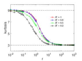
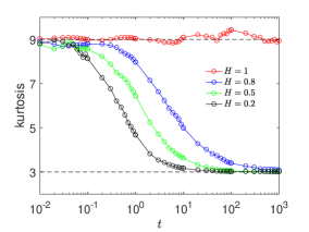
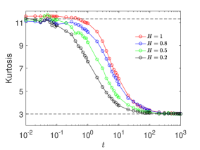
Figure 5: Langevin simulations of the kurtosis for the three random-diffusivity models: (a) FBM-DD, (b) FBM-TC, (c) FBM-S. Parameters of the FBM-S model: $D_{1}=1$, $D_{2}=0.01$, $k_{12}=3/4$, and $k_{21}=1/4$.

References

References

- [1] N. van Kampen, Stochastic processes in physics and chemistry (North Holland, Amsterdam, 1981).
- [2] B. Wang, J. Kuo, S. C. Bae, and S. Granick, Nat. Mater. 11, 481 (2012); B. Wang, S. M. Anthony, S. C. Bae, and S. Granick, Proc. Natl. Acad. Sci. USA 106, 15160 (2009); J. Guan, B. Wang, and S. Granick, ACS Nano 8, 3331 (2014).
- [3] K. He, F. B. Khorasani, S. T. Retterer, D. K. Tjomasn, J. C. Conrad, and R. Krishnamoorti, ACS Nano 7, 5122 (2013).
- [4] C. Xue, X. Zheng, K. Chen, Y. Tian, and G. Hu, J. Phys. Chem. Lett. 7, 514 (2016); D. Wang, R. Hu, M. J. Skaug, and D. Schwartz, J. Phys. Chem. Lett. 6 54 (2015); S. Dutta and J. Chakrabarti, EPL 116, 38001 (2016).
- [5] K. C. Leptos, J. S. Guasto, J. P. Gollub, A. I. Pesci, and R. E. Goldstein, Phys. Rev. Lett. 103, 198103 (2009).
- [6] A. V. Chechkin, F. Seno, R. Metzler, and I. M. Sokolov, Phys. Rev. X 7, 021002 (2017).
- [7] A. G. Cherstvy, O. Nagel, C. Beta, and R. Metzler, Phys. Chem. Chem. Phys. 20, 23034 (2018).
- [8] C. Beck and E. G. D. Cohen, Physica A 332, 267 (2003).
- [9] M. V. Chubynsky and G. W. Slater, Phys. Rev. Lett. 113, 098302 (2014).
- [10] R. Jain and K. L. Sebastian, J. Phys. Chem. B 120, 3988 (2016); J. Chem. Sci. 129, 929 (2017).
- [11] N. Tyagi and B. J. Cherayil, J. Phys. Chem. B 121, 7204 (2017).
- [12] V. Sposini, A. V. Chechkin, F. Seno, G. Pagnini, and R. Metzler, New J. Phys. 20, 043044 (2018).
- [13] Y. Lanoiselée, N. Moutal, and D. S. Grebenkov, Nat. Comm. 9, 4398 (2018).
- [14] A. Sabri, X. Xu, D. Krapf, and M. Weiss, E-print arXiv:1910.00102.
- [15] D. S. Grebenkov, Phys. Rev. E 99, 032133 (2019).
- [16] S. Burov and E. Barkai, Phys. Rev. Lett. 124, 060603 (2020).
- [17] M. Hidalgo-Soria and E. Barkai, E-print arXiv:1909.07189.
- [18] E. B. Postnikov, A. Chechkin, and I. M. Sokolov, New J. Phys., at press.
- [19] V. Sposini, D. S. Grebenkov, R. Metzler, G. Oshanin, and F. Seno, E-print arXiv:1911.11661.
- [20] J. Szymanski and M. Weiss, Phys. Rev. Lett. 103, 038102 (2009).
- [21] J.-H. Jeon, N. Leijnse, L. B. Oddershede, and R. Metzler, New J. Phys. 15, 045011 (2013).
- [22] J.-H. Jeon et al, Phys. Rev. Lett. 106, 048103 (2011).
- [23] G. Guigas, C. Kalla, and M. Weiss, Biophys. J. 93, 316 (2007).
- [24] S. C. Weber, A. J. Spakowitz, and J. A. Theriot, Phys. Rev. Lett. 104, 238102 (2010).
- [25] J. F. Reverey, J.-H. Jeon, H. Bao, M. Leippe, R. Metzler, and C. Selhuber-Unkel, Sci. Rep. 5, 11690 (2015).
- [26] J.-H. Jeon, H. Martinez-Seara Monne, M. Javanainen, and R. Metzler, Phys. Rev. Lett. 109, 188103 (2012); G. R. Kneller, K. Baczynski, and M. Pasienkewicz-Gierula, J. Chem. Phys. 135, 141105 (2011).
- [27] I. Goychuk, Phys. Rev. E 80, 046125 (2009); Adv. Chem. Phys. 150, 187 (2012).
- [28] R. Metzler, J.-H. Jeon, A. G. Cherstvy, and E. Barkai, Phys. Chem. Chem. Phys. 16, 24128 (2014).
- [29] E. Lutz, Phys. Rev. E 64, 051106 (2001); G. Kneller, J. Chem Phys. 141, 041105 (2014).
- [30] B. B. Mandelbrot and J. W. van Ness, SIAM Rev. 10, 422 (1968).
- [31] H. Qian, in Processes with long-range correlations: theory and applications, edited by G. Rangarajan and M. Z. Ding, Lecture Notes in Physics vol 621 (Springer, New York, 2003).
- [32] S. Thapa, N. Lukat, C. Selhuber-Unkel, A. Cherstvy, and R. Metzler, J. Chem. Phys. 150, 144901 (2019).
- [33] T. J. Lampo, S. Stylianido, M. P. Backlund, P. A. Wiggins, and A. J. Spakowitz, Biophys. J. 112, 532 (2017).
- [34] J.-H. Jeon, M. Javanainen, H. Martinez-Seara, R. Metzler, and I. Vattulainen, Phys. Rev. X 6, 021006 (2016).
- [35] I. Munguira, I.Casuso, H. Takahashi, F. Rico, A. Miyagi, M. Chami, and S. Scheuring, ACS Nano 10, 2584 (2016); S. Gupta, J. U. de Mel, R. M. Perera, P. Zolnierczuk, M. Bleuel, A. Faraone, and G. J. Schneider, J. Phys. Chem. Lett. 9, 2956 (2018); W. He, H. Song, Y. Su, L. Geng, B. J. Ackerson, H. B. Peng, and P. Tong, Nat. Commun. 7, 11701 (2016).
- [36] J. Ślȩzak, R. Metzler, and M. Magdziarz, New J. Phys. 20, 023026 (2018); E. van der Straeten and C. Beck, Physica A 390, 951 (2011).
- [37] J. Yu, J. Xiao, X. Ren, K. Lao, and X. S. Xie, Science 311, 1600, (2006).
- [38] C. di Rienzo et al., Nature Comm. 5, 5891 (2014).
- [39] M. S. Song, H. C. Moon, J.-H. Jeon, and H. Y. Park, Nat. Comm. 9, 344 (2018); K. Chen, B. Wang, and S. Granick, Nature Mat. 14, 589 (2015).
- [40] D. Robert, T. H. Nguyen, F. Gallet, and C. Wilhelm, PLoS ONE 4, e10046 (2010).
- [41] A. Caspi, R. Granek, and M. Elbaum. Phys. Rev. Lett. 85, 5655 (2000).
- [42] G. Seisenberger, U. Ried, T. Endreß, H. Büning, M. Hallek, and C. Bräuchle, Science 294, 1929 (2001); B. Brandenburg and X. Zhuang, Nat. Rev. Microb. 5, 197 (2007); E. Sun, J. He, and X. Zhuang, Curr Opin Virol. 3, 34 (2013).
- [43] O. Pulkkinen and R. Metzler, Phys. Rev. Lett. 110, 198101 (2013); A. B. Kolomeisky, Phys. Chem. Chem. Phys. 13, 2088 (2011).
- [44] A. B. Kolomeisky and M. E. Fisher, Ann. Rev. Phys. Chem. 58, 675 (2007); P. M. Hoffmann, Rep. Prog. Phys. 79, 032601 (2016); I. Goychuk, V. O. Kharchenko, and R. Metzler, Phys. Chem. Chem. Phys. 16, 16524 (2014).
- [45] S. L. Heston, Rev. Fin. Stud. 6, 327 (1993).
- [46] O. El Euch and M. Rosenbaum, Math. Fin. 29, 3 (2019).
- [47] S. Thapa, M. A. Lomholt, J. Krog, A. G. Cherstvy, and R. Metzler, Phys. Chem. Chem. Phys. 20, 29018 (2018).
- [48] A. P. Prudnikov, J. A. Bryčkov and O. I. Maričev, (Gordon and Breach, London, UK, 1998)