On the Equivalence of Neural and Production Networks

Abstract

This paper identifies the mathematical equivalence between economic networks of Cobb-Douglas agents and Artificial Neural Networks. It explores two implications of this equivalence under general conditions. First, a burgeoning literature has established that network propagation can transform microeconomic perturbations into large aggregate shocks. Neural network equivalence amplifies the magnitude and complexity of this phenomenon. Second, if economic agents adjust their production and utility functions in optimal response to local conditions, market pricing is a sufficient and robust channel for information feedback leading to macro learning.

1 Introduction

There is a burgeoning literature surrounding the network origins of aggregate shocks. Network economics can model how an individual’s behavior effects the society in which she is embedded (Goyal, 2015). Several mathematical frameworks have been proposed that amplify microeconomic fluctuations into large macroeconomic movements (Acemoglu et al., 2012, 2015) which would otherwise be modeled as exogenous shocks. This paper’s core innovation is that it identifies a more natural and flexible mathematical model than previously examined. This model is intrinsic to existing theory. Specifically, economic networks of Cobb-Douglas agents facing nonlinear inverse demand functions are mathematically equivalent to Artificial Neural Networks (ANNs.)

We survey the pertinent mathematics at the intersection of the two disciplines of Economics and Machine Learning to demonstrate this equivalence. We explore two implications of modeling the economy as a Neural Network (NN) under general conditions. The first is a consequence of the functional completeness of NNs: neither the amplitude nor complexity of an aggregate “shock” in response to a given microeconomic input can be reasonably bounded. Any conceivable functional form is possible. Second, if the producers and consumers are free to adjust their production and utility functions in optimal response to local conditions, market pricing is a sufficient and robust channel for information feedback leading to global, macro-scale learning. This learning is at the level of the economy as a whole and is transparent to the individual producers and consumers.

Below, we first develop the mathematical equivalence between production units and ANNs. Then we address the endogeneity/exogeneity of macro shocks, and finally we discuss global learning behavior.

2 Cobb-Douglas Producers and Artificial Neurons

We posit that the Cobb-Douglas producers behave like Artificial Neural Networks for two reasons. First, the microeconomic agents are mathematically analogous to artificial neurons, the fundamental components of ANNs. Second, the microeconomic agents interact with each other in a way that is mathematically analogous to the interactions between neurons in an ANN. To demonstrate this equivalence, we will begin with the ANN neuron.

ANN neurons combine weighted input signals, which are the outputs of other neurons, in a nonpolynomial fashion. Theoretically, the inputs can be weighted in any fashion (exponentially, polynomially, etc.), but in practice what we call a Standard Artificial Neuron (SAN) takes the form of Equation 1 (Minsky et al., 2017).

$$P_{i}=a(b_{i}+\mathbf{\omega}_{i}\mathbf{\cdot p}_{k}),$$ (1)

where $a(x)$ is an “activation function”; $\mathbf{p}_{k}$ is a vector of output values from the previous layer $k$; $\mathbf{\omega}_{i}$ is a vector of “synaptic weights” or coefficients belonging to neuron $i$; $b_{i}$ is a “bias” belonging to neuron $i$; and $P_{i}$ is the output of neuron $i$. $P_{i}$ is destined to be one of the entries in the vector $\mathbf{p}_{k+1}$ to be used in the next layer.

The activation function, $a(x)$, can take many forms, with different functions having different properties, but as long as the activation function is nonpolynomial an ANN with linear weights will function (Cybenko, 1989; Ritter and Sussner, 1996).

Due to a number of desirable properties, one commonly used activation function is the “Softplus” function expressed in Equation 2 (Glorot et al., 2011):

$$\sigma\left(x\right)=\ln\left(1+e^{x}\right)$$ (2)

We will modify this equation slightly:

$$a(x)=-\sigma(x)=\ln\left(\frac{1}{1+e^{x}}\right)$$ (3)

This will have the exact same properties as the Softplus, but it will reflect the output around the x-axis. This inversion has no effect on the network because the following layer’s neurons can neutralize it by inverting the sign of their weight vectors. The ANN neuron specification using the inverted Softplus is equivalent (with the constraints we discuss below) to a profit maximizing, price-taking Cobb-Douglas producer facing an unknown inverse demand of the form:

$$\rho(Y_{i})=\frac{1}{1+Y_{i}}$$ (4)

Here $Y_{i}$ is the fully differentiated but substitutable output of producer i and $\rho(Y_{i})$ yields the price of each unit of $Y_{i}$. This inverse demand function is not mathematically necessary for economic agents to form an ENN, but it has reasonable theoretical properties: It exhibits a fixed maximum price, is decreasing in $Y$, and approaches zero asymptotically.

Now we examine the Cobb-Douglas Producer-cum-neuron in the ENN. Let $m$ be an index corresponding to a neuron in the previous layer; $A$ be the “technology parameter”; $x_{ji}$ be the input quantity demanded by producer $i$ for the jth good; $\alpha_{ji}$ be the exponent in i’s Cobb-Douglas function parameterizing the jth good; $P_{i}$ be the price that producer i expects to get for each unit of her output at the time of her production decision; $p_{j}$ be the price per unit of input j.

The Decreasing Returns to Scale (DRS) Cobb-Douglas production function is:

$$Y_{i}=A_{i}\prod_{m=1}^{n}x_{mi}^{\alpha_{mi}},$$ (5)

where $x_{mi},\alpha_{mi}>0,\Phi_{i}<1,$ and where $\Phi_{i}\equiv\sum\limits_{m=1}^{n}\alpha_{mi}$ and $\eta_{i}\equiv\Phi_{i}-\alpha_{1i}.$ The profit function is:

$$\pi_{i}=P_{i}Y_{i}-\sum_{m=1}^{n}p_{m}x_{mi}.$$ (6)

Maximizing profit, the first order conditions give us equations 7 and 8:

$$x_{1,i}=\left[\left(P_{i}A_{i}\right)^{-1}\left(\frac{p_{1}}{\alpha_{1i}}\right)^{1-\eta_{i}}\prod\limits_{m=2}^{n}\left(\frac{p_{m}}{\alpha_{mi}}\right)^{\alpha_{mi}}\right]^{\frac{1}{\Phi_{i}-1}}.$$ (7)

$$x_{mi}=x_{1i}\frac{p_{1}\alpha_{mi}}{p_{m}\alpha_{1i}}$$ (8)

The ENN model requires output in terms of prices alone. Inserting equations 7 and 8 into equation 5 yields equation 9:

$$Y_{i}=\left[P_{i}^{-\Phi_{i}}A_{i}^{-1}\prod\limits_{m=1}^{n}\left(\frac{p_{m}}{\alpha_{m,i}}\right)^{\alpha_{m,i}}\right]^{\frac{1}{\Phi_{i}-1}}.$$ (9)

Transforming 9 into logs yields equation 10:

$$\ln Y_{i}=\sum_{m=1}^{n}\frac{\alpha_{mi}}{\Phi_{i}-1}\ln p_{m}+\frac{\Phi_{i}\ln P_{i}+\ln A_{i}+\sum_{m=1}^{n}\alpha_{mi}\ln\alpha_{mi}}{1-\Phi_{i}}.$$ (10)

Now, let $\omega_{m}\equiv\frac{\alpha_{mi}}{\Phi_{i}-1}$, let $\omega$ be the vector of all $\omega_{m}$, let $l\equiv\ln p$ calculated elementwise (that is, the vector of log input prices,) let

$$z_{i}=\frac{\Phi_{i}\ln P_{i}+\ln A_{i}+\sum_{m=1}^{n}\alpha_{mi}\ln\alpha_{mi}}{1-\Phi_{i}},$$

and let the log price of output, $L_{i}\equiv\ln\rho\left(Y_{i}\right)=\ln\left(\frac{1}{1+Y_{i}}\right)$ by (7). Then $\ln Y_{i}=\mathbf{l}_{k}\mathbf{\cdot\omega}_{k}+z_{i}$ and $a\ln Y_{i}=L_{i}$ by (6), and the price of the good output by a Cobb-Douglas producer can be modelled in logs with equation 11:

$$L_{i}=a\left(\mathbf{l}_{k}\mathbf{\cdot\omega}_{k}+z_{i}\right).$$ (11)

This is the standard ANN neuron as expressed in 1. In the ENN context, the market prices of the producers’ inputs are equivalent to neuronal input values and the price of the producer’s output is equivalent to neuronal output values. Although the mathematical model we show specifically invokes the Cobb-Douglas producer, the equivalence between an economic agent (whether goods producer or labor producing consumer) and an ANN neuron is general and robust to production, utility, and inverse demand function specifications. As long as the price of an output good cannot be expressed as a linear combination of the prices of input goods, the production of that output good within a network of similar production activities creates a functionally complete network.

3 Functional Completeness

As we mentioned above, the Cobb-Douglas has constraints that do not bind the ANN neuron. The exponents of the production function, $\alpha_{mi}$, must be greater than zero and the function we specified must be DRS, that is, $\Phi_{i}$ must be less than one (DRS is required so that the profit maximization process we use is valid). Therefore, the weights $\omega_{mi}$ are strictly less than zero. This limits the ENN’s learning potential compared to an ANN which can have both positive and negative weights. As our computer simulation shows below, this constraint does not fully remove the ENN’s ability to learn. Nor is this constraint evident in real world production functions. It is an artifact of the Cobb-Douglas, which we have chosen because of its prominence as a theoretical standard rather than for empirical reasons.

Our choice of the sub-optimal Cobb-Douglas specification serves as both a robustness test of ENN behavior and a nod to canonical economic theory. We use it exclusively in our simulations for those reasons. A more realistic ENN model, however, would include heterogenous household utility functions and firm production functions that inherently overcome the limitations imposed by homogenous Cobb-Douglas producers. In order to demonstrate how easily a practical ENN specification can emulate the full range of ANN behavior, we consider the NAND gate.

The NAND gate is functionally complete, and since a simple single hidden layer NN can emulate the NAND gate, Neural Networks are also functionally complete by extension. This means that all possible logical functions can be approximated to an arbitrary degree of precision by an NN (Abu‐Mostafa, 1986; Leshno et al., 1993; Ritter and Sussner, 1996). This argument is most intuitive when using neurons with Heaviside step activation functions, but it is well understood in the field that functional completeness extends naturally to Standard Artificial Neurons with differentiable activation functions as specified above. The SAN does not output two discreet values, but the values can be interpreted as probabilities with an actionable probability threshold. If a neuron outputs a value greater than or equal to the threshold, it can be interpreted as the binary 1 (or electronic HIGH, or logical TRUE), and if below the threshold, it can be interpreted as the binary 0 (or electronic LOW, or logical FALSE).

NAND Truth Table

Input 1 Input 2 Output

$0$ $0$ $1$

$0$ $1$ $1$

$$1 0 1$$

$$1 1 0$$

Because the synaptic weights of the Cobb-Douglas Producer Neuron (CDPN) in equation 11 are strictly negative, it cannot form a NAND gate. Neither can it form a NOT gate, which could be used in series with an AND or OR gate to build a functionally complete network. In order to establish the feasibility of a functionally complete ENN, we will specify parameters of a CDPN to form an AND gate and then specify a Cobb-Douglas-like production function and parameters to form a NOT gate. The NOT gate can then be joined in series with the AND to form the functionally complete NAND gate.

One example set of parameters with which a two-input CDPN can emulate an AND gate is as follows (here using a sigmoid activation function: $a(x)=\ln\left(\frac{1}{1+e^{x}}\right)):$

$\alpha_{1}=\alpha_{2}=\frac{20}{41}\qquad P_{i}=1\qquad A=\frac{e^{\frac{30}{41}}}{\alpha_{1}^{\Phi}}.$

Therefore, $\omega_{1}=\omega_{2}=-20,$ and $z=30.$ Let this CDPN be called producer (or agent or neuron) $X.$ Let the producer emulating the NOT gate be called the $\Psi$ neuron.

Let $\Psi$ have the capability of producing one of two products, $Y_{3}$ or $Y_{4}$, each using CD functions with a single input. But due to the production technology employed, $\Psi$ cannot produce both $Y_{3}$ and $Y_{4}$. Optimal output of each product is calculated by $\Psi$, and she then chooses to produce the product with the greater profit at that optimal level, thereby forgoing any production of the less profitable product. This production function satisfies the following expressions:

$$(Y_{3}=0)\vee\left(Y_{4}=0\right)$$ (12)

and

$$\left(Y_{j}=A_{j}x_{j}^{\alpha_{j}}\right)\vee\left(Y_{j}=0\right)\text{ for }j=3,4.$$ (13)

Using the same process that transformed 5 into 11 above, 13 can be re-expressed in terms of output prices, in logs:

$$\ln\rho\left(Y_{j}\right)=a\ln Y_{j}=a(\omega_{j}\ln p_{j}+z_{j})\vee 1=L_{j}\text{ for }j=3,4.$$ (14)

Producer $\Psi$, as expressed in (17) has two outputs, $L_{3}$ and $L_{4}$, and two inputs, $p_{3}$ and $p_{4}.$If input $p_{4}$ is constant (or varies within a range, or has less volatility than $p_{3}$) the parameters of $\Psi$ can be set so that its output $L_{4}$ and input $p_{3}$ form a NOT gate.

One set of parameters with which $\Psi$ can emulate a NOT gate (when $\ln p_{4}\approx 0$) is as follows:

$P_{3},$ $P_{4}=1,\alpha_{3}=\frac{1}{2}$, $A_{3}=3,$ $\alpha_{4}=1-e^{-10},$ $A_{4}=\frac{1}{(1-\alpha_{4})^{1-\alpha_{4}}\alpha_{4}^{\alpha_{4}}}.$

Combining agents $X$ and $\Psi$ with the parameters listed above into a simple two neuron network yields a functioning NAND gate. Let the output of $X$ be $L_{3}\equiv\ln p_{3}$. That is, the output product of $X$ is the first input of $\Psi$. The output of this network is shown below in truth-table format. Since the NAND gate is functionally complete, any ENN which incorporates producers who can shift production between two or more products may also be functionally complete. Of course, other conceivable production functions can yield the same results. The only requirement is that some of the producers in the network experience, within some range of conditions, circumstances in which an increase in the price of one or more of their inputs induces an increase in the output of one or more of their products.

NAND gate ENN (with agents $$X$$ and )

lnp₁ lnp₂ Inp₃ lnp₄ L₄

(logical input 1) (logical input 2) ( (assumed const.) (

0 0 1

0 0 1

0 0 1

1 0 0

  

4 Complex Behavior in Simple Networks

Next we explore how small, local shocks can propagate through an ENN to generate sometimes highly surprising aggregate behaviors. Here we build upon the arguments of Vasco Carvalho (2014), who uses network structures to “confront a deep-seated and influential logic which, to this day, justifies the continued appeal to an exogenous synchronization device, in the form of aggregate shocks.” Our model amplifies Carvalho’s reasoning. When a laborer takes maternity or bereavement leave or contracts a serious illness, or when a company changes hands through inheritance, these micro shocks are not necessarily lost in the random noise of the aggregate economy. Instead, they can become important signals which reverberate through the markets and change the direction of the economy as a whole.

A modern economy can be described as an intricate system of networks in which consumers and producers interact via reasonably efficient markets. Within these networks, small changes directly affecting only a small set of producers within a sector of the economy may translate to large and unforeseeable changes in the aggregate. This system is too complex to describe in detail, and impossible to model explicitly using standard economic models. Standard models often aggregate heterogeneity into distributions according to various assumptions and thereby lose this important feature of the economy they seek to model. Attempts have been made, however, to better understand the inner workings of production networks and how micro shocks in them produce macroeconomic fluctuations (see e.g. Acemoglu et al. (2012), Carvalho (2014)).

Here we are considering a world where explicit modeling is not possible due to the complexity of the various networks that comprise the economy. A key feature is to retain the idiosyncrasies that characterize real economies and how they propagate through the network, producing sometimes unpredictable, inexplicable, and, not seldom, unintended consequences.

For tractability, we specifically consider a simple network architecture with one input, one hidden layer, and a dual output. The set-up is inspired by Rosenblatt’s perceptron model in which binary classifiers learn to recognize patterns through an algorithm when fed training data (Rosenblatt, 1961). Our model is a slightly modified version of the original perceptron. The network is one directional so there are no feedback loops. Consequently, unlike the perceptron model, learning cannot occur. Output seems quite random, yet follows logical principles that are unobservable. Outside empirical data can be fitted to the model, and this data would be consistent with reality. But naturally, this data will be overfitted. Standard models rely on exogenous variation (i.e., exogenous shocks) to explain e.g. aggregate business cycle fluctuations – here these fluctuations arise naturally from individual changes in behavior that may occur for endogenous reasons.

Figure 1: The four models in figure 2 are Cobb Douglas producer networks. The so-called hidden layer has five producers in models two and three and ten producers in models one and four. Hidden layer members are either intermediate good producers or leisure good producers. These goods are inputs to the network’s final output producer. All hidden layer production functions take the form $Y_{i}=A_{i}x^{\alpha_{i}}$ where $x$ is the quantity of the sole raw material required to produce intermediate and leisure goods in this economy, $Y_{i}$ is output, and $A_{i}$ is the technology parameter. The network’s final producer outputs $Y_{l}=A_{l}\prod_{k=1}^{K}{{x_{k}}^{a_{k}}}\$ where $l\in$ {Intermediate, Leisure} and $k$ is the index of the $k$th labor or leisure good (as applicable).

We use a basic Cobb-Douglas technology in which a single input price is fed to a set of up to ten producers who produce intermediate goods to the final producer in the economy. The final producer then chooses between two kinds of outputs. We illustrate the ratio of these two outputs in Figure 2 on page 2 with respect to the price of the input commodity. In order for the impacts of these behaviors to be as clear as possible, it is helpful to imagine the two products are Labor and Leisure. Suppose the final producer is a hot dog vendor choosing whether to provide snacks at a baseball game or instead to take a seat and watch the Red Sox fight off their arch rivals (who shall remain nameless.) The modification of the vendor’s production function or the cascading effects of modifications to intermediate producers’ production functions lead to unforeseen and sometimes highly unpredictable and non-monotonic changes in the labor/leisure decision of the vendor. In other words, unscalable individual decisions produce aggregate outcomes that could not be easily modeled within the canonical neoclassical framework.

Figure 2 illustrates four examples of the hot dog vendor network. Relatively small changes to the producers’ production functions alter the output ratio considerably, and in highly unpredictable ways. Two things are worth noticing. First, the hot dog vendor behaves almost erratically as the input price changes. The ratio of Labor to Leisure takes very different values in a relatively small input range. Second, small changes in the Cobb-Douglas parameters yield substantial changes in the shape of the graphs. This again underlines the difficulty of predicting output variation caused by production changes in the hot dog technology.

Of course the choices of a single hot dog vendor are not enough to move the needle on national unemployment or GDP figures. But the capacity of this type of network to generate and transmit these erratic behaviors only increases with the network’s complexity. When Labor and Leisure choices are writ large, unpredictable behavior can be catastrophic.

Figure 2: The simple single-hidden-layer network architecture (inspired by Rosenblatt”s perceptron) used in these functions is described in figure 1. See table LABEL:funkyGraphParams for initial parameters.
These hypothetical (but feasible) labor/leisure ratio functions are nonmonotonic, even chaotic. As the log price of the single raw material increases, the functions change regimes sharply and unpredictably. An observer without a network-based economic model must describe such regime changes as exogenous shocks. An additional source of such shocks is also illustrated here: adjustments to the initial model parameters. These can cause unexpected and counterintuitive changes to the labor/leisure ratio function both in level and in shape.
The dashed line denotes the initial parameters, the dotted line (where present) denotes intermediate parameters, and the solid line denotes the final parameters.

Table 1: *

Model	Product Type	$A^{Int/Leis}_{i}$	$\alpha^{Int/Leis}_{i}$	$A^{out}_{l}$	$\alpha^{out}_{lk}$
Model 1	Intermed	9	0.675	1.684	0.091
	”	0.022	0.954		0.091
	”	0.389	0.964		0.13
	”	5,066	0.265		0.091
	”	2.2	0.53		0.01
	Leisure	11	0.53	1.5	0.01
	”	0.083	0.974		0.083
	”	2.399	0.964		0.091
	”	85.516	0.742		0.001
	”	22	0.53		0.142
Model 2	Intermed	0.002	0.909	1.6	0.375
	”	50	0.95		0.01
	”	0.383	0.98		0.057
	Leisure	0.406	0.968	1.5	0.091
	”	0.002	0.98		0.091
Model 3	Intermed	0.005	0.909	847.277	0.111
	”	41.389	0.909		0.067
	”	41.389	0.909		0.067
	Leisure	0.439	0.909	0.1	0.111
	”	34,600,299	0.909		0.067
Model 4	Intermed	47.275	0.476	6.009	0.01
	”	41.389	0.455		0.01
	”	2,105	0.417		0.01
	”	0.003	0.49		0.048
	”	0.541	0.484		0.038
	Leisure	34,600,299	0.455	1.5	0.01
	”	2.707	0.455		0.02
	”	0.002	0.455		0.231
	”	0.383	0.49		0.029
	”	5,530	0.476		0.005
The network’s’ initial parameters are described as follows: $A^{Int/Leis}_{i}$ refers to the Cobb Douglas technology parameter of the ith intermediate or ith leisure good, $\alpha_{i}^{Int/Leis}$ refers to the CD exponent on the sole (raw material) input of the ith intermediate or ith leisure good. $A_{l}^{out}$ refers to the technology parameters of the output producer, and $\alpha_{lk}^{out}$ refers to the output producer’s exponent on the kth input of type $l$ where $l\in$ {Intermediate, Leisure}.

5 A Simple Model of a Learning Economic Neural Network

Imagine the fictional country of Islandia, a small, isolated nation. Its economy is driven by the import of raw materials and the export of finished goods.

Islandia’s imports consist of only two products: raw steel and brass. The country uses these two raw materials to fashion intermediate goods which are in turn used to fashion its single export commodity, clockwork chess players. Each month, a cargo ship from the nearest Economic Super-Power offloads a shipment of brass and steel and hauls away a load of Mechanical Turks to be sold in catalogs, websites, and shopping malls. It takes exactly one month for the small nation to convert brass and steel into chess players.

The producers in Islandia form a simple hierarchy. Eight work with the raw steel and brass to create tools, tubing, spring steel, gear blanks, cog blanks, and the like. These eight producers are the first level in the economy, and their only inputs are the two imported raw materials. There are then eight producers in the second level using some of each of the first level’s products as inputs. Levels three and four each have eight more producers who use the previous level’s outputs as inputs. The eight outputs of level four are the sub-components used by the single level-five producer to make clockwork chess players. So there are 33 individual producers in Islandia, all of whom are organized into well-defined layers where 32 producers manufacture intermediate goods, and one producer manufactures the final good.

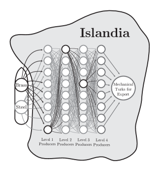
Figure 3: Input/Output matrix of Islandia economy. Arbitrary producers are highlighted for visual clarity.

The producers in Islandia all have Cobb-Douglas production functions of the form:

$$Y=A\prod_{i=1}^{n}x_{i}^{\alpha_{i}},$$ (15)

where $A$ is a technology parameter shared with all of the producers within the same layer. The producers each attempt to maximize their own profits:

$$\pi=PY-\sum_{i=1}^{n}p_{i}x_{i}^{\alpha_{i}},$$ (16)

where $\mathit{P}$ is the anticipated price (the price the producer believes she will get for her finished good at the time she makes her production choices), $p_{i}$ is the price of the input commodity $x_{i}$, and $n$ is the number of input commodities (always eight except for the first layer, where it is two).

Prices are set through Walrasian tatonnement. Therefore, the accuracy of the anticipated price cannot be known at the time of production. The actual price manufacturer $m$ receives for her output minus the price she expected to receive gives $m$ a value for her “pricing error.” She uses the pricing error to estimate her production error – that is, the amount that she over or under produced. This production error could also be called, using the terminology of Artificial Neural Networks (ANN’s), her “cost function.” She is motivated to minimize this cost function, and makes two types of adjustments to do so.

Once the producer has calculated her cost function, she first adjusts her anticipated price. She uses a simple moving average for this adjustment. Next, she employs a single step of the gradient descent procedure to make small adjustments to the exponents in her production function (Ruder, 2016). She is able to make these adjustments through slight changes to the processes and technologies that she employs.

Let $E$ be the production error, or cost, let $\partial Y/\partial\alpha_{i}$ be the partial derivative of output with respect to exponent $\alpha_{i}$, and let $\mu$ be a “learning rate” parameter. Using gradient descent, producer $m$ will update each of the exponents of her production function according to the rule:

$$\alpha_{i}^{\prime}=\alpha_{i}-E\mu\frac{\partial Y}{\partial\alpha_{i}}.$$ (17)

All manufacturers on Islandia use the same learning process as producer $m$. Their information set does not allow any of them to make adjustments to their production based on the quantities of imports to or exports from the nation – but together, their economy forms an ENN that defines and refines decision boundaries – regions of the two-dimensional (brass and steel) import quantity map for which different production levels are preferred.

The arrangement of the interconnections between neurons in a Neural Network (NN) is known as the Neural Architecture (Misra and Saha, 2010; Svozil et al., 1997). Islandia has a simple “Feed Forward” architecture – that is, each neuron outputs only to neurons on the next layer. There are no outputs to neurons of the same or previous layers. Feed Forward networks can vary by the number of “hidden layers” (a term referring to all layers except the input and output layers – the Brass and Steel and the Mechanical Turks in Islandia) and also the number of neurons in each layer.

Figure 4: Maps of the six training dataset result values as a function of input quantities. For odd numbered datasets the shaded region is true and the unshaded region is false, vice-versa for even numbered datasets. Each training dataset consists of 100 periods worth of randomly generated input-result vector pairs. The 2D input vector consists of quantities imported of steel and brass and the 1D boolean result vector is true if demand in the period is higher than average. Using dataset 1 as an example, let the randomly generated input vector be 40 units of steel and 40 units of brass. The map defines the matching output vector as true. In contrast, dataset 5 would map the same point to false.

We note that the ENN on Islandia performs very poorly by Artificial Neural Network standards. Unlike the NN’s used in Artificial Intelligence applications, the economy of the little nation is not optimized for network performance. Every agent optimizes their choices based only on the local price feedback mechanism (the local error), not on the component share in the global error (as calculated by Islandia’s export market and final producer – as would be the case in an efficient ANN.) Because price information must trickle down the network layer by layer, the information a producer uses to adjust production is delayed by several periods compared to the information that was used to direct that production. This phase delay scrambles much of the information about the economy’s overall optimization problem and prevents the country’s ENN from learning to predict with accuracies that rival ANNs. Economies more realistic than Islandia’s are not as highly constrained. Price is not the only information channel available to most producers. Economic reports, stock market performance, communication with suppliers and customers, and other business news sources give each producer direct information about global system performance.

Another factor that prevents Islandia’s ENN from approaching the performance of an optimized ANN is that the Cobb Douglas production functions are strictly increasing with respect to the input quantity of goods. As discussed above, neurons within ANNs use functions that can be either increasing or decreasing, as needed, with respect to their inputs. This means, for example, that Islandia cannot manufacture more Mechanical Turks in response to a shortage in both steel and brass – even if the corresponding increase in steel and brass prices consistently signals a boom in demand for clockwork chess players next period. Although realistic ENN models can overcome this limitation, we keep it in place for Islandia in order to test learning behavior under the most restrictive assumptions.

All Neural Networks, whether ANNs, biological systems, or ENNs, are subject to trouble with local optima. This is certainly an issue faced by each of Islandia’s producers and the country as a whole, but there is another notable and idiosyncratic barrier to learning in Islandia. Every producer has complete medium and long-term memory loss. Therefore each producer can make exactly one adjustment to their production function per period based only on the information in front of them. This is equivalent to a hyper-restricted “online learning” paradigm in an ANN (Misra and Saha, 2010; Svozil et al., 1997). High-power ANNs, however, typically use “batch-learning” processes. In batch-learning, the error function is calculated from a large number of training examples (in Islandia’s case, periods) simultaneously. This is advantageous because a single training example might lead a Neural Network to update in such a way that it improves performance for that single example but degrades performance for all others. Given the further possibility of local optima, this means Islandia’s online learning paradigm will sometimes lead to network “unlearning” – that is, training decreases performance rather than improves it. Fortunately, most real-world producers have a memory so this is only a problem in Islandia. In summary, the Islandia model we test here is as suboptimal for learning as possible while still capable of testing whether prices are a sufficient information channel for online learning. Our strategy is to isolate the price feedback mechanism as the source of training information while removing standard features of ANNs which would otherwise be strong assumptions in an economic model. If the model exhibits global learning from price feedback under standard and weak assumptions, it is certainly capable of learning under stronger and more optimized assumptions.

Table 2: *

	Initial Accuracy	Post-training Accuracy	Training Improvement
	(Std. Error)	(Std. Error)	(t-score)
Dataset 1	20.15%	32.2%	12.05%**
	(0.69%)	(3.35%)	(3.3503)
Dataset 2	76.35%	90.3%	13.95%***
	(1.34%)	(0.5624%)	(9.586)
Dataset 3	70.2%	76.85%	6.65%***
	(0.73%)	(1.0495%)	(5.1905)
Dataset 4	27.65%	79.1%	51.45%***
	(0.84%)	(0.764%)	(45.2923)
Dataset 5	49.7%	54.8%	5.1%*
	(1.13%)	(2.0424%)	(2.1865)
Dataset 6	49.05%	54%	4.95%**
	(1.10%)	(1.4654%)	(2.7024)
Average Percent Accuracy of Islandia’s ENN before and after training using the six different datasets illustrated in in Figure 4 on page 4. Each result is the average of 20 independent trials with random initialization of the ENN’s parameters. Training Improvement is defined as (Percent Accuracy post-training) minus (Percent Accuracy pre-training).
*,**,and *** denote greater than 95%, 99%, and 99.99% confidence rejection of the one-sided null hypothesis of no average training improvement.

Even with Islandia’s limitations its economy shows a remarkable ability to learn. Its output changes in response to patterns in the input prices. Although this learning is driven by individual microeconomic optimization choices, the individual producers are unaware learning is occurring. It happens in the aggregate, on the macroeconomic level, and not on the level of the producers who drive it.

Islandia is worth studying in this regard because of the simple structure of its economy. We are able to create a precise and tractable computer model by which to simulate its learning performance. The learning response of the model of Islandia’s economy with six different datasets is reported in Table LABEL:learningPerformance. The datasets consist of $100$ periods of import supply and export demand data randomly generated to conform to the patterns in Figure 4 on page 4. For each period there is a pair of input quantities (representing raw steel and brass), each ranging between $0$ and $100$, and a Boolean value assigned to “true” if Islandia can expect higher than normal demand for its clockwork chess players. The six datasets each exhibit a different pattern determining which regions of the input / output map are true and which regions are false. The ENN attempts to converge to a different optimal decision boundary for each dataset.

We initialized twenty independent model economies for each dataset, and in each case trained the economies over $600$ randomly drawn rounds (each round consisting of a single training example from the dataset.) To measure learning, we first define the threshold output quantity as the average output of the untrained economy across a subset of the training set inputs. We then interpret an output above this threshold as corresponding to the Boolean true value and an output below the threshold as corresponding to Boolean false. The Percent Accuracy of the network is the proportion of output true/false values that match the input true/false values. We define a simple measure of learning performance as the increase in Percent Accuracy – that is, the Percent Accuracy of the trained network minus the Percent Accuracy of the untrained network.

Learning performance is reported in Table LABEL:learningPerformance on page LABEL:learningPerformance. Using dataset $1$, the ENN Percent Accuracy increased $12.1\%$ on average. This was the most difficult dataset for the ENN to respond to since lower input quantities of the raw materials needed to correspond with higher output quantities of the finished good. With dataset $2$, Percent Accuracy increased $14.0\%$ on average and with dataset $3$ it increased $6.7\%$. However, for reasons that are the inverse of the limitations on dataset $1$, the untrained ENNs performed very well on these datasets from the outset – both datasets averaging over $70\%$ before training. Therefore there was less room for improvement from training. Dataset $2$ yielded the highest average performance of all the datasets after training, at $90.3\%$ Percent Accuracy. Dataset $4$ yielded an accuracy increase of $51.5\%$. This was the dataset that elicited the strongest learning response and the second highest absolute accuracy after training, $79.1\%$. Datasets $5$ and $6$ have the most convoluted optimal decision boundaries. They would likely benefit from a larger network since the ability of a NN to converge to a complex and convoluted decision boundary increases with the size of the network. Nevertheless, the ENN exhibited learning behavior. Dataset $5$ accuracy increased by $5.1\%$ and dataset $6$ accuracy increased by $5.0\%.$

6 Concluding remarks

Our macroeconomic understanding, until now, has been rooted in smooth functions of aggregations of microeconomic agents. The possibility of emergent economic phenomena has been implicitly recognized for some time, but our assumptions may have inadvertently suppressed their study by offering no mechanism for emergent behaviors to arise. We have analyzed two critical examples of this. The endogeneity of apparently exogenous shocks can be easily masked by the complexity of the ENN’s network interactions. Furthermore, because an ENN is capable of learning en masse, economic structures (i.e. traditions, norms, or institutions) may evolve which provide benefit to an aggregation without apparently providing utility to the individual agents involved. Further study of these interactions may yield novel insights into market failures like the Tragedy of the Commons, unfavorable game theoretical equilibria, and persistent informal structures such as race-based discrimination and inter-generational poverty.

Our studies of the ENN model are just beginning. Perhaps the most promising implication of the ENN model is its use in government and NGO policy formation. The ENN’s learning behavior implies that policies might employ active training techniques to affect change. We cannot say with confidence that this is possible – but the prospect is tantalizing enough to motivate further study. It may be possible to identify a training ‘handle’ – by which we mean an input through which to deliver rewards and punishments – and a low latency data source to observe an economic response to the varying economic landscape. In which case, regional and local economic reforms could be affected through training policies perhaps as simple as high frequency subsidy level adjustment.

We do not assert the ENN model supplants the canonical smooth models in any way. These two models are complementary and coexist without conflict. Here we appeal to the mathematical analogy between biological brains and ANN’s, which is quite robust. Medical science has learned much about the biological brain, has employed powerful medical imaging, and has used effective surgical and pharmacological techniques based solely on aggregate approaches. Virtually no medical technology currently relies on the precise identification of the synaptic weights of individual neurons. Aggregate measures for diagnosis and prediction – in both the biological brain and the ENN – will likely always be superior. Measurement precision and computing power are finite. But the complexity of a Neural Network is vast and perfect precision – an impossibility – would be required to accurately predict its output. A simplified model cannot predict the output of a Neural Network. Therefore, models of the ENN can only illuminate certain aspects of its behavior. These are the topics of further research.

References

- (1)
- Abu‐Mostafa (1986) Abu‐Mostafa, Yaser S. (1986) “Neutral networks for computing?” AIP Conference Proceedings, 151 (1), 1–6.
- Acemoglu et al. (2012) Acemoglu, Daron, Vasco M. Carvalho, Asuman Ozdaglar, and Alireza Tahbaz-Salehi (2012) “The Network Origins of Aggregate Fluctuations,” Econometrica, 80 (5), 1977–2016.
- Acemoglu et al. (2015) Acemoglu, Daron, Asuman Ozdaglar, and Alireza Tahbaz-Salehi (2015) “Networks, Shocks, and Systemic Risk,”Technical report.
- Carvalho (2014) Carvalho, Vasco M. (2014) “From Micro to Macro via Production Networks,” Journal of Economic Perspectives, 28 (4), 23–48.
- Cybenko (1989) Cybenko, G. (1989) “Approximation by superpositions of a sigmoidal function,” Mathematics of Control, Signals, and Systems, 2 (4), 303–314.
- Glorot et al. (2011) Glorot, Xavier, Antoine Bordes, and Yoshua Bengio (2011) “Deep Sparse Rectifier Neural Networks,” in Gordon, Geoffrey, David Dunson, and Miroslav Dudík eds. Proceedings of the Fourteenth International Conference on Artificial Intelligence and Statistics, 15 of Proceedings of Machine Learning Research, 315–323, Fort Lauderdale, FL, USA: PMLR, 11–13 Apr.
- Goyal (2015) Goyal, S. (2015) “Networks in Economics: A Perspective on the Literature.”
- Leshno et al. (1993) Leshno, Moshe, Vladimir Ya. Lin, Allan Pinkus, and Shimon Schocken (1993) “Multilayer feedforward networks with a nonpolynomial activation function can approximate any function,” Neural Networks, 6 (6), 861–867.
- Minsky et al. (2017) Minsky, Marvin, Seymour Papert, and Bottou Leon (2017) Perceptrons: an introduction to computational geometry: The MIT Press.
- Misra and Saha (2010) Misra, Janardan and Indranil Saha (2010) “Artificial neural networks in hardware: A survey of two decades of progress,” Neurocomputing, 74 (1-3), 239–255.
- Ritter and Sussner (1996) Ritter, G.X. and P. Sussner (1996) “An introduction to morphological neural networks,” in Proceedings of 13th International Conference on Pattern Recognition: IEEE.
- Rosenblatt (1961) Rosenblatt, Frank (1961) Principles of neurodynamics. perceptrons and the theory of brain mechanisms: Defense Technical Information Center.
- Ruder (2016) Ruder, Sebastian (2016) “An overview of gradient descent optimization algorithms.”
- Svozil et al. (1997) Svozil, Daniel, Vladimir Kvasnicka, and Jiri Pospichal (1997) “Introduction to multi-layer feed-forward neural networks,” Chemometrics and Intelligent Laboratory Systems, 39 (1), 43–62.