Thresholded Adaptive Validation:
Tuning the Graphical Lasso for Graph Recovery

Abstract

Many Machine Learning algorithms are formulated as regularized optimization problems, but their performance hinges on a regularization parameter that needs to be calibrated to each application at hand. In this paper, we propose a general calibration scheme for regularized optimization problems and apply it to the graphical lasso, which is a method for Gaussian graphical modeling. The scheme is equipped with theoretical guarantees and motivates a thresholding pipeline that can improve graph recovery. Moreover, requiring at most one line search over the regularization path, the calibration scheme is computationally more efficient than competing schemes that are based on resampling. Finally, we show in simulations that our approach can improve on the graph recovery of other approaches considerably.

Thresholded Adaptive Validation: Tuning the Graphical Lasso for Graph Recovery

Mike Laszkiewicz, Asja Fischer, Johannes Lederer

Thresholded Adaptive Validation:
Tuning the Graphical Lasso for Graph Recovery

Mike Laszkiewicz &Asja Fischer &Johannes Lederer

Department of Mathematics, Ruhr University Bochum, Germany

1 Introduction

Over the last decades full of technical achievements, we experienced a revolutionary supply of data, confronting us with large-scale data sets. In order to handle and to infer new insights from the appearing wealth of data it presupposes us to put effort into the development of new, scaleable procedures. One approach to address this problem is using graphical models, which proved to serve as an intuitive, easy-understanding visualization of the underlying interaction network that can then be further analyzed. Typical applications for graphical models occur in several modern sciences, including genetics Dobra et al. (2004), the analysis of brain connectivity networks Bu and Lederer (2017), and the investigation of complex financial networks Denev (2015). In all of these cases, graphical models can reduce the network of interactions to its relevant parts to lighten the challenge of high-dimensionality. While domain experts can analyze and interpret the structure of interactions across features, we can use this information for more accurate model building. Using a sparse representation of the relevant parts of the model, it is possible to develop more efficient inference algorithms and accelerate sampling from the model. A popular approach to face this challenge is to recover the network from the data using undirected graphical models. We call this task graph recovery.

An important class of undirected graphical models are Gaussian graphical models. There are numerous estimators for Gaussian graphical models, including those that account for high dimensionality, e.g. the graphical lasso Yuan and Lin (2007); Banerjee et al. (2007); Friedman et al. (2008), SCAD Fan et al. (2009), and MCP Zhang (2010), which are based on the idea of regularized maximum likelihood estimation, and various other approaches such as neighborhood regression Meinshausen and Bühlmann (2006); Sun and Zhang (2012), TIGER Liu and Wang (2017), and SCIO Liu and Luo (2015). These estimators reduce the effective dimensionality of the model through a regularization term that is adjusted to the setting at hand with a regularization parameter.

In this paper we generalize the theoretical framework of Chichignoud et al. (2014) and utilize the large body of preliminary theoretical work Ravikumar et al. (2011) to verify that we can apply this general scheme to the graphical lasso. Important features of the resulting data-driven calibrated estimator are that it comes with a finite sample upper bound on the approximation error and is computationally efficient as it requires at most one graphical lasso solution path. We equip the estimator with a simple, theory-based threshold and observe a significant improvement over other methods in its graph recovery performance.

The rest of the paper is organized as follows. Section 2 briefly reviews Gaussian graphical models and presents the proposed estimator for graph recovery, which we call thresholded adaptive validation graphical lasso (thAV). Based on an empirical analysis of toy data sets presented in Section 3, we demonstrate that the thAV outperforms existing methods on the graph recovery tasks. We apply the thAV to real-world data to recover biological networks in Section 4. Finally, we conclude with a discussion and present ideas for future research in Section 5. The supplement contains theoretical results, proofs, and further simulations. The code for our experiments is provided and can further be accessed through our public git repository.

2 Thresholded Adaptive Validation for the Graphical Lasso

We begin by giving a brief review of Gaussian graphical models and describing the graphical lasso optimization problem in Section 2.1. In Section 2.2 we apply the adaptive validation (AV) calibration scheme, which was originally proposed by Chichignoud et al. (2014) and which we generalize to general regularized optimization problems in Section A.1 of the supplement, to the graphical lasso. We obtain finite sample results for the $\ell_{\infty}$-loss on the off-diagonals of the graphical lasso, and employ these bounds to motivate a thresholded graphical lasso approach.

2.1 Brief Review of Gaussian Graphical Models

An undirected graphical model expresses the conditional dependence structure between components of a multivariate random variable. More precisely, given a high-dimensional random variable $\boldsymbol{z}\in\mathbb{R}^{d}$, the undirected graphical model depicts for each pair of components $z_{i},\,z_{j}$ of $\boldsymbol{z}$ if these are independent given the remaining $d-2$ components of $\boldsymbol{z}$ (i.e.  $z_{i}\perp z_{j}|\boldsymbol{z}_{\backslash\{i,j\}}$). Formally, an undirected graphical model is defined as a pair $(\boldsymbol{z},\mathcal{G})$, where $\mathcal{G}:=(\mathcal{V},\mathcal{E})$ is a graph with vertices $\mathcal{V}:=\{1,...,d\}$ and edge set $\mathcal{E}:=\{(i,j)\in\mathcal{V}\times\mathcal{V}:\;z_{i}\not\perp z_{j}|\boldsymbol{z}_{\backslash\{i,j\}}\}$. It is well-known that in a Gaussian graphical model, i.e. in the case that $\boldsymbol{z}\sim\mathcal{N}_{d}(\boldsymbol{0}_{d},\,\Sigma)$, where $\Sigma$ is the positive definite covariance matrix, we can find an elegant characterization of the conditional dependency structure. It can be seen as a special case of the Hammersley-Clifford Theorem Grimmett (1973); Besag (1974); Lauritzen (1996): for any $i\neq j\in\mathcal{V}$ it holds that

$$z_{i}\perp z_{j}|\boldsymbol{z}_{\backslash\{i,j\}}\quad\Leftrightarrow\quad\Theta_{ij}=0\enspace,$$ (1)

where $\Theta:=\Sigma^{-1}$ is the so called precision matrix. Hence, in order to estimate the conditional dependence graph $\mathcal{G}$, one can build on an estimate $\hat{\Theta}$ of the precision matrix $\Theta$ and define $\hat{\mathcal{E}}:=\{(i,j)\in\mathcal{V}\times\mathcal{V}:\;\hat{\Theta}_{ij}\neq 0\}$.

Given $n$ samples $\boldsymbol{z}^{(1)},\dots,\,\boldsymbol{z}^{(n)}$ drawn independently from $\mathcal{N}_{d}(\boldsymbol{0}_{d},\,\Sigma)$, an evident approach to estimate $\Theta$ is to employ maximum likelihood estimation. But it is well-known that its performance suffers in the high-dimensional setting where $n\approx d$ or even $n<d$, and that it does not exist in the latter setting Wainwright (2019). A typical approach to overcome the burdens that come with high-dimensionality is to assume a sparsity structure on the target, that is, to assume $\Theta$ to have many zero-entries. This does not only improve theoretical guarantees but also makes the conditional dependence graph more interpretable. Moreover, imposing a sparsity structure is in accordance with the scientific beliefs in typical application areas in which graphical models are being used Thieffry et al. (1998); Jeong et al. (2001). The probably most-frequently used sparsity encouraging estimation procedure for Gaussian graphical models is the graphical lasso Yuan and Lin (2007)

$$\hat{\Theta}_{r}=\operatorname*{\arg\!\min}_{\Omega\in\operatorname*{\mathcal{S}_{d}^{+}}+}\biggl{\{}\operatorname{tr}\biggl{[} \frac{1}{n}\sum_{i=1}^{n}\bigl{(}\boldsymbol{z}^{(i)}\bigr{)}^{\top}\boldsymbol{z}^{(i)}\Omega\biggr{]}$$

$$-\log\left[\det[\Omega]\right]+r\|\Omega\|_{1,\operatorname{off}}\biggr{\}}\enspace,$$ (2)

where $\operatorname*{\mathcal{S}_{d}^{+}}+$ is the set of positive definite and symmetric matrices in $\mathbb{R}^{d\times d}$, $\operatorname{tr}$ denotes the trace, $r$ is a problem-dependent regularization parameter, and $\|\Omega\|_{1,\operatorname{off}}:=\sum_{i\neq j}|\Omega_{ij}|$ denotes the $\ell_{1}$-norm of $\Omega\in\operatorname*{\mathcal{S}_{d}^{+}}+$ on its off-diagonal. Of course, the performance of the estimator hinges on the choice of $r$, and while general theoretical results for the graphical lasso exist (e.g. those presented by Zhuang and Lederer (2018)), to the best of our knowledge there are none that allow for a sophisticated choice of $r$ for graph recovery tasks that occur in practice.

2.2 Thresholded Adaptive Validation

In this section, we transfer the AV technique proposed by Chichignoud et al. (2014) for the lasso to the graphical lasso. As can be seen from our derivation in Section A.1 of the supplement, the technique can be applied to tune any general regularized optimization problem over a set $\mathbb{S}$ of the form

$$\hat{\Theta}_{r}\in\operatorname*{\arg\!\min}_{\Omega\in\mathbb{S}}\bigl{\{}f(\boldsymbol{Z},\Omega)+rh(\Omega)\bigr{\}}\enspace,$$ (3)

where $r$ is a real-valued regularization parameter, $f$ is a function measuring the fit of the estimator $\Omega$ given the observed data $\boldsymbol{Z}$, and $h$ is some regularization function depending only on $\Omega$. Comparing (2) with (3) shows that the graphical lasso belongs to this class of regularized optimization problems. We can therefore apply the calibration scheme proposed by Chichignoud et al. (2014) and which we generalized in the supplement to obtain the following definition:

Definition 1 (AV).

Let $\mathcal{R}$ be a finite and nonempty set of regularization parameters. Then, the adaptive validation (AV) calibration scheme selects the regularization parameter according to

$$\hat{r}:=\min\bigl{\{}r\in\mathcal{R}:\;\ell\bigl{(}\hat{\Theta}_{r^{\prime}} ,\hat{\Theta}_{r^{\prime\prime}}\bigr{)}\leq C(r^{\prime}+r^{\prime\prime})$$

$$\quad\quad\forall\,r^{\prime},r^{\prime\prime}\in\mathcal{R}\cap[r,\infty)\bigr{\}}\enspace,$$

where $\ell:\mathcal{S}_{d}^{+}\times\mathcal{S}_{d}^{+}\rightarrow\mathbb{R}$ is the $\ell_{\infty}$-distance on the off-diagonals, $C\in\mathbb{R}$ is a constant (specified in the following), and $\hat{\Theta}_{r^{\prime}},\,\hat{\Theta}_{r^{\prime\prime}}$ are the graphical lasso estimators (2) using regularization parameter $r^{\prime}$ and $r^{\prime\prime}$, respectively. We call $\hat{\Theta}_{\hat{r}}$ (resulting from inserting $\hat{r}$ into (2)) the AV estimator.

The constant $C$ stems from an assumption, which the theory of Chichignoud et al. (2014) relies on, namely that there exists this constant and a class of events $(\mathcal{T}_{r})_{r\in\mathcal{R}}$, which are increasing in $r$, such that conditioned on $\mathcal{T}_{r}$ it holds

$$\ell(\Theta,\hat{\Theta}_{r})\leq Cr\enspace.$$ (4)

Particularly, we only require the existence of the set of events $(\mathcal{T}_{r})_{r\in\mathcal{R}}$ for some fixed $C$ and do not need to have access to it. As demonstrated by Theorem 8 in Section A.2 of the supplement, we can show based on the investigations of Ravikumar et al. (2011) that this assumption holds true for the graphical lasso. Motivated by this, the smallest regularization parameter $r_{\delta}^{\ast}$ that enables us to apply (4) with probability $1-\delta$, for some $\delta\in(0,1]$, can be seen as a natural candidate for $r$:

$$r_{\delta}^{\ast}:=\operatorname*{\arg\!\min}_{r\in\mathcal{R}}\left\{\mathbb{P}\bigl{(}\mathcal{T}_{r}\bigr{)}\geq 1-\delta\right\}\enspace.$$

However, $r_{\delta}^{\ast}$ is inaccessible in practice, since we usually cannot measure $\mathbb{P}(\mathcal{T}_{r})$. Nonetheless, the AV estimator $\hat{\Theta}_{\hat{r}}$ also results in a good approximation of the precision matrix as guaranteed by the following theorem, which is based on the generalization of the Theorem 3 of Chichignoud et al. (2014) applied onto the graphical lasso.

Theorem 2 (Finite Sample Bound for the AV).

Suppose that $\hat{r}$ is the regularization parameter selected by the AV calibration scheme and $C$ is the constant from (4). Then, for any $\delta\in(0,1]$, it holds that

$$\hat{r}\leq r_{\delta}^{\ast}\quad\textrm{ and }\quad\ell\bigl{(}\Theta,\hat{\Theta}_{\hat{r}}\bigr{)}\leq 3Cr_{\delta}^{\ast}$$ (5)

with probability at least $1-\delta$.

For simplicity of notation, let us denote the AV estimator by $\hat{\Theta}:=\hat{\Theta}_{\hat{r}}$ from here on. The finite sample upper bound (5) immediately implies that it holds with probability $1-\delta$ that

1. for any zero entry $\Theta_{ij}=0$ of the true precision matrix the corresponding entry $\hat{\Theta}_{ij}$ of the AV estimate satisfies $|\hat{\Theta}_{ij}|\in[0,3Cr_{\delta}^{\ast}]$;

2. for any significant non-zero entry $\Theta_{ij}$ with $|\Theta_{ij}|>(3+\lambda)Cr_{\delta}^{\ast}$, for some constant $\lambda$, the corresponding entry $\hat{\Theta}_{ij}$ of the AV estimate is also non-zero with $|\hat{\Theta}_{ij}|>\lambda Cr_{\delta}^{\ast}$.

These observations suggest a strategy for efficient graph recovery: by including all edges $(i,j)$ to the edge set that satisfy $|\hat{\Theta}_{ij}|>\lambda Cr_{\delta}^{\ast}$, we make sure that we recover all significant entries (see 2.). Pursuing this strategy, we can also shrink the interval, in which AV missclassifies zero entries to $[\lambda Cr_{\delta}^{\ast},\,3Cr_{\delta}^{\ast}]$ (see 1.). However, as $r_{\delta}^{\ast}$ is inaccessible, we propose to replace it in the selection strategy by the AV regularization parameter, leading to the thresholded estimator defined in the following.

Definition 3 (thAV).

Let $\hat{\Theta}$ be the $AV{}$ estimator. Then, we define the thresholded adaptive validation graphical lasso (thAV) estimator by

$$\bigl{(}\hat{\Theta}^{t}\bigr{)}_{ij}:=\bigl{(}\hat{\Theta}_{ij}\mathds{1}_{\{|\hat{\Theta}_{ij}|>t\}}\bigr{)}_{ij}\enspace,$$ (6)

where $t:=\lambda C\hat{r}$ is the threshold, $\lambda\in(0,3]$, and $\mathds{1}_{A}$ is the indicator function over a set $A$. The resulting estimated edge set is then

$$\hat{\mathcal{E}}: =\bigl{\{}(i,j)\in\mathcal{V}\times\mathcal{V}:\;\hat{\Theta}_{ij}^{t}\neq 0\bigr{\}}$$

$$=\bigl{\{}(i,j)\in\mathcal{V}\times\mathcal{V}:\;|\hat{\Theta}_{ij}|>\lambda C\hat{r}\bigr{\}}\enspace.$$

As we know from Theorem 2 that $\hat{r}\leq r_{\delta}^{\ast}$ with probability $1-\delta$, we can use the above observations to derive the following corollary that guarantees outstanding graph recovery properties of the thAV:

Corollary 4 (Finite Sample Graph Recovery).

Let $\hat{\Theta}$ be the AV estimator and $\hat{\Theta}^{t}$ the thAV estimator with $t=\lambda C\hat{r}$, where $C$ is the constant from Assumption (4) and $\lambda\in(0,3]$. Then, it holds with probability $1-\delta$ that

1. for all $(i,j)\in\mathcal{V}$ such that $\Theta_{ij}=0$ it is ${|\hat{\Theta}_{ij}|\in[0,\,3Cr_{\delta}^{\ast}]}$ and therefore

   $$(i,j)\in\hat{\mathcal{E}}\iff|\hat{\Theta}_{ij}|\in(\lambda C\hat{r},\,3Cr_{\delta}^{\ast}]\enspace.$$

2. for all $(i,j)\in\mathcal{V}$ such that $|\Theta_{ij}|>(3+\lambda)Cr_{\delta}^{\ast}$ it is $(i,j)\in\hat{\mathcal{E}}$.

The proof of Corollary 4 can be found in Section A.3 of the supplement. As far as we know, there is no other theoretical result so far that justifies a specific choice for a threshold in a thresholded version of the graphical lasso. Moreover, the corollary offers a theoretical ground for balancing the tradeoff between false positive and false negative rate: while maintaining finite-sample guarantees, we can regulate $\lambda$ according to our needs to decrease the false negative rate (part $2$) at the cost of increasing the interval $(\lambda C\hat{r},3Cr_{\delta}^{\ast}]$ in which thAV missclassifies negatives (part $1$).

Importantly, the thAV also comes with notable computational benefits, since the computations in Definition 1 only require at most $1$ solution path. Using the glasso R package Friedman et al. (2008); Witten et al. (2011), we can efficiently compute the thAV as described by Algorithm 1 in Section B of the supplement.

Finally, note that even though there exist theoretical bounds justifying (4) (see Section A.2 of the supplement), they are usually too loose or bounded to restrictions that are hard to interpret and violated in practice. Thus, what we observe in practice is usually not (4), but rather a more robust “quantiled version” of it:

$$\ell_{1-\alpha}(\Theta,\hat{\Theta})\leq Cr\enspace,$$

where $\ell_{1-\alpha}(\Theta,\hat{\Theta})$ defines the $1-\alpha$ quantile of the set of absolute differences $\{|\Theta_{ij}-\hat{\Theta}_{ij}|\}_{ij}$. Under this assumption, one could derive the same theory for the quantiled version of the loss, i.e. by replacing all $\ell$ by $\ell_{1-\alpha}$ in this section (compare with the general theory in Section A.1 of the supplement). However, in practice the results are very similar and our method is computationally less expensive.

3 Simulation study

In this section we compare the thAV to various other commonly used methods to estimate a Gaussian graphical model, which are the StARS Liu et al. (2010), the scaled lasso Sun and Zhang (2012), the TIGER Liu and Wang (2017), the regularized score matching estimator (rSME) tuned via eBIC Lin et al. (2016), and the SCIO tuned via CV and via the Bregman-criterion Liu and Luo (2015). We sample synthetic data from a Gaussian distribution $\mathcal{N}_{d}(\boldsymbol{0}_{d},\,\Theta^{-1})$, whereby we adopt a similar precision matrix generation procedure from Caballe et al. (2015) for sampling random and scale-free graphs. A detailed description of the based generation process can be found in Section C.1 of the supplement. We scale the data such that it is centered and has empirically unit variance.

If not stated differently, we use $t=C\hat{r}$ and $C=0.7$ in the following. We define the set of possible regularization parameters to be $\mathcal{R}:=\{0.05+i(r_{\operatorname{max}}-0.05)/40:\;i\in\{1,...,40\}\}$, where $r_{\operatorname{max}}:=\max_{i\neq j}|\hat{\Sigma}_{ij}|$ is the largest off-diagonal entry in absolute value of the empirical covariance matrix. To enhance the robustness of our algorithm, we scale the graphical lasso estimators in Definition 1 such that they have unit diagonal entries. If not specified, the results of all experiments are averaged over $25$ iterations and standard deviations are shown in parenthesis. Besides the experiments presented in this paper, we present additional investigations and repeat all experiment in various settings in Section C.3 of the supplement. We provide the code for all experiments with the submission, which can further be accessed through the public git repository.

Performance in $F_{1}$-score

Table 1: Graph recovery performance for varying graphs and sample size. The bold numbers indicate the best score in each setting.

		random				scale-free
		$F_{1}$	Precision	Recall		$F_{1}$	Precision	Recall
$n=300,\,d=200$
oracle		0.70 (0.13)	0.60 (0.16)	0.89 (0.03)		0.37 (0.12)	0.37 (0.22)	0.63 (0.23)
StARS		0.59 (0.14)	0.44 (0.13)	0.93 (0.09)		0.29 (0.13)	0.20 (0.10)	0.65 (0.12)
scaled lasso		0.68 (0.02)	0.52 (0.03)	0.98 (0.01)		0.40 (0.07)	0.26 (0.05)	0.84 (0.07)
TIGER		0.47 (0.09)	0.31 (0.08)	$\boldsymbol{0.99}$ (0.01)		0.34 (0.07)	0.21 (0.05)	$\boldsymbol{0.87}$ (0.07)
rSME (eBIC)		0.64 (0.17)	0.49 (0.16)	0.98 (0.01)		0.47 (0.23)	0.42 (0.24)	0.74 (0.14)
scio (CV)		0.19 (0.36)	0.23 (0.41)	0.17 (0.34)		0.15 (0.19)	0.44 (0.50)	0.09 (0.12)
scio (Bregman)		0.13 (0.17)	0.11 (0.22)	0.96 (0.16)		0.24 (0.18)	$\boldsymbol{0.51}$ (0.44)	0.57 (0.37)
thAV		$\boldsymbol{0.91}$ (0.03)	$\boldsymbol{0.90}$ (0.04)	0.93 (0.05)		$\boldsymbol{0.54}$ (0.13)	0.48 (0.19)	0.70 (0.13)
$n=200,\,d=300$
oracle		0.70 (0.10)	0.63 (0.14)	0.81 (0.03)		0.29 (0.07)	0.25 (0.15)	0.47 (0.13)
StARS		0.54 (0.11)	0.39 (0.11)	0.93 (0.03)		0.25 (0.07)	0.17 (0.06)	0.54 (0.10)
scaled lasso		0.65 (0.03)	0.49 (0.02)	0.94 (0.02)		$\boldsymbol{0.30}$ (0.04)	0.20 (0.03)	0.59 (0.08)
TIGER		0.45 (0.08)	0.30 (0.07)	0.96 (0.02)		0.25 (0.05)	0.15 (0.04)	0.67 (0.09)
rSME (eBIC)		0.02 (0.00)	0.01 (0.00)	$\boldsymbol{0.99}$ (0.01)		0.01 (0.00)	0.01 (0.00)	$\boldsymbol{0.95}$ (0.02)
scio (CV)		0.00 (0.00)	0.00 (0.00)	0.00 (0.00)		0.06 (0.09)	0.36 (0.49)	0.03 (0.05)
scio (Bregman)		0.26 (0.29)	0.27 (0.35)	0.86 (0.21)		0.16 (0.12)	$\boldsymbol{0.57}$ (0.47)	0.36 (0.27)
thAV		$\boldsymbol{0.79}$ (0.09)	$\boldsymbol{0.73}$ (0.15)	0.90 (0.04)		0.28 (0.11)	0.21 (0.14)	0.60 (0.11)
$n=400,\,d=200$
oracle		0.74 (0.13)	0.65 (0.17)	0.91 (0.03)		0.42 (0.10)	0.42 (0.22)	0.67 (0.26)
StARS		0.63 (0.13)	0.48 (0.14)	0.96 (0.03)		0.34 (0.12)	0.23 (0.09)	0.70 (0.14)
scaled lasso		0.70 (0.03)	0.54 (0.03)	0.99 (0.01)		0.44 (0.05)	0.29 (0.04)	0.90 (0.07)
TIGER		0.48 (0.09)	0.32 (0.08)	0.99 (0.01)		0.33 (0.05)	0.20 (0.04)	$\boldsymbol{0.93}$ (0.06)
rSME (eBIC)		0.56 (0.20)	0.41 (0.18)	$\boldsymbol{1.00}$ (0.00)		0.54 (0.13)	0.43 (0.15)	0.82 (0.11)
scio (CV)		0.48 (0.45)	0.52 (0.47)	0.48 (0.46)		0.14 (0.25)	0.28 (0.45)	0.10 (0.19)
scio (Bregman)		0.16 (0.16)	0.12 (0.22)	0.97 (0.13)		0.21 (0.18)	0.35 (0.40)	0.71 (0.36)
thAV		$\boldsymbol{0.93}$ (0.04)	$\boldsymbol{0.92}$ (0.06)	0.95 (0.04)		$\boldsymbol{0.63}$ (0.13)	$\boldsymbol{0.59}$ (0.19)	0.75 (0.14)

Table 1 shows the performance of the different methods for the graph recovery task. The performance is evaluated based on precision, recall, and the resulting $F_{1}$-score, which are defined in Section C.3 of the supplement. The proposed thAV estimator not only clearly outperforms the baseline methods but it also has a noticeable advantage over the oracle graphical lasso estimator, which is the (non-thresholded) graphical lasso estimator that achieves maximal $F_{1}$-score among all regularization parameters. This implies that it is mandatory to apply thresholding on top of regularized optimization to obtain good graph recovery results with the graphical lasso. Remarkably, in estimating a random graph, we observe that the thAV always achieves a recall of above $0.9$ while maintaining good precision. This is in stark contrast to the other methods, which seem to overestimate the graphs resulting in a high recall but comparably low precision. Moreover, the results indicate that scale-free graphs in general are much harder to estimate than random graphs. As it has already been reported in other works (see Liu and Ihler (2011); Tang et al. (2015) and references therein), the graphical lasso is not able to provide a good estimation of a scale-free graph because its regularization does not impose any preference for identifying hub-like structures. Nevertheless, thAV remains superior to the other methods in terms of reaching the highest $F_{1}$-Score in most cases. Again, thAV can find a good balance between precision and recall, whereas methods such as StARS and TIGER are overestimating the graph, which results in comparably low precision.

Table 2: Graph recovery performance of the thAV with fixed sample size $n=500$ for large-scale examples. The results are based on $20$ iterations.

		random				scale-free
		$F_{1}$	Precision	Recall		$F_{1}$	Precision	Recall
$d=600$		0.96 (0.03)	0.97 (0.02)	0.94 (0.05)		0.43 (0.17)	0.45 (0.29)	0.61 (0.17)
$d=700$		0.96 (0.02)	0.98 (0.02)	0.93 (0.04)		0.42 (0.16)	0.43 (0.25)	0.53 (0.13)
$d=800$		0.95 (0.02)	0.97 (0.03)	0.93 (0.04)		0.40 (0.18)	0.45 (0.29)	0.52 (0.16)
$d=900$		0.96 (0.02)	0.97 (0.04)	0.95 (0.03)		0.33 (0.17)	0.33 (0.26)	0.54 (0.16)
$d=1000$		0.96 (0.02)	0.98 (0.01)	0.93 (0.03)		0.34 (0.17)	0.36 (0.27)	0.46 (0.15)

In Table 1, it appears that the recovery performance drops with an increment of $d$, which makes sense since the number of parameters increases quadratically with $d$. However, in our next experiments (Table 2), in which we investigate the thAV in the setting $d\in\{600,\dots,1000\}$ and set $n=500$, we observe that this is surprisingly not the case when enough data, but still $n<d$, is available. The $F_{1}$-score for a random graph remains stable across all $d$ at an impressive value of $0.96$. In the case of a scale-free graph, the performance decays slowly, while maintaining a good trade-off between precision and recall. Note that the support recovery in the case $d=1000$ involves about $500\,000$ parameters.

Moreover, the careful reader will actually realize that the proposed calibration scheme can also be employed to tune the rSME estimator. Because of the generality of our results from Section A.1 we can employ existing results from Lin et al. (2016) to verify the validity of Assumption (4) for the rSME. As it is shown in Section C.4 of the supplement, the rSME calibrated with the thAV approach performs comparably to the thAV graphical lasso. This is an important observation as the rSME can be applied to estimate the conditional dependency structure of a pairwise interaction model, which is a broader model class than the class of Gaussian graphical models. Hence, the calibration technique and the underlying theory can naturally be extended to the non-Gaussian setting.

Furthermore, we repeat the empirical study with the modified graphical lasso proposed by Liu and Ihler (2011), which we calibrate and clip via the thAV technique. This estimator employs a power law regularization that encourages the appearance of nodes with a high degree and are thus better suited for scale-free graphs. The experimental study is shown in Section C.4 of the supplement.

Dependence on $C$

If we increase the constant $C$ in the AV calibration scheme, we decrease $\hat{r}$ (see Proposition 9 of the supplement) and therefore employ less regularization. Hence, the AV estimator is inherently related to the choice of $C$. We plot the performance of different AV estimators with varying thresholds in Figure 1 and make two crucial observations. First, we see significant dissimilarities in the performance of the unthresholded AV estimators: because the calibrated regularization parameter ranges from $\hat{r}=0.23$ in the case $C=0.5$ to $\hat{r}=0.09$ in the case $C=0.8$, the $F_{1}$-score drops from approximately $0.70$ to $0.35$. Thus, the AV estimator’s performance heavily depends on the choice of $C$. But after thresholding, and this is the second observation, the thresholded AV estimators’ performance curves become very similar and reach almost the same peak. We can observe the same behaviour in the other settings, as it is shown in Section C.3 of the supplement. Importantly, we also show in the supplement that we do not observe a similar performance peak if we threshold the unregularized optimization problem (setting $r=0$ in (2)). Hence, neither regularization via regularized optimization is sufficient for graph recovery, see the performance of the oracle estimator in Table 1, nor does unregularized thresholding yield to good results. Therefore we claim that it is necessary to apply both types of regularizations, as it is done by thAV and which additionally encourages stability in $C$.

To further investigate the stability of the thAV in $C$, we consider pairs of thAV estimators resulting from different choices of $C$, which we call $\hat{\Theta}_{C^{\prime}}^{t^{\prime}}$ and $\hat{\Theta}_{C^{\prime\prime}}^{t^{\prime}}$. Table 3 reports the differences between these estimators by calculating $F_{1}(\hat{\Theta}_{C^{\prime}}^{t^{\prime}},\hat{\Theta}_{C^{\prime\prime}}^{t^{\prime}})$ for a random graph. We do not only achieve a high $F_{1}(\Theta,\,\hat{\Theta}_{C}^{t})$ for any $C$, but also the different estimates are all very similar, i.e. $F_{1}(\hat{\Theta}_{C^{\prime}}^{t},\,\hat{\Theta}_{C^{\prime\prime}}^{t})$ is always above $0.80$. Therefore, we can confirm that the recovered graphs are stable in the choice of $C$.

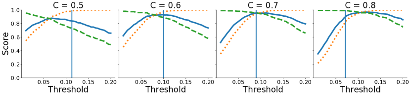
Figure 1: The $F_{1}$-score (blue, solid), precision (yellow, dotted), and recall (green, dashed) of a thresholded AV estimator for a random graph with $d=200$ based on $n=300$ samples for $C\in\{0.5,\,0.6,\,0.7,\,0.8\}$ with varying thresholds. The resulting AV regularization parameters are $0.23,\,0.17,\,0.13,\,0.09$, respectively. The vertical line depicts the proposed threshold $t=C\hat{r}$ corresponding to the thAV estimate.

Table 3: Similarity $F_{1}(\hat{\Theta}_{C^{\prime}}^{t},\hat{\Theta}_{C^{\prime\prime}}^{t})$ for different choices of $C$ ($C^{\prime}$ and $C^{\prime\prime}$) for a random graph with $d=200$ using $n=300$ samples. The performance scores $F_{1}(\Theta,\hat{\Theta}_{C}^{t})$ are $0.80\,(0.06),\;0.88\,(0.04),\;0.91\,(0.05),\;0.85\,(0.10)$ for $C$ in $0.5,\;0.6,\;0.7,\;0.8$, respectively.

$C$		0.6	0.7	0.8
0.5		0.88 (0.05)	0.82 (0.08)	0.81 (0.10)
0.6		1	0.93 (0.04)	0.84 (0.09)
0.7		-	1	0.92 (0.05)
0.8		-	-	1

Varying graph density

Table 4: $F_{1}$-score if we change the connection probability to $p\in\{2/d,\,4/d\}$ in a random graph in various settings. The previous simulations employed $p=3/d$. The bold numbers indicate the best score in each setting.

		$2/d$	$4/d$
$n=300,\,d=200$
StARS		0.55 (0.14)	0.57 (0.13)
scaled lasso		0.60 (0.03)	0.73 (0.02)
TIGER		0.39 (0.09)	0.53 (0.08)
rSME (eBIC)		0.51 (0.27)	0.55 (0.23)
SCIO (CV)		0.33 (0.40)	0.22 (0.39)
SCIO (Bregman)		0.23 (0.29)	0.22 (0.23)
thAV		$\boldsymbol{0.91}$ (0.05)	$\boldsymbol{0.89}$ (0.04)
$n=200,\,d=300$
StARS		0.49 (0.11)	0.52 (0.09)
scaled lasso		0.58 (0.03)	0.68 (0.02)
TIGER		0.35 (0.09)	0.48 (0.10)
rSME (eBIC)		0.01 (0.00)	0.03 (0.00)
SCIO (CV)		0.14 (0.26)	0.20 (0.31)
SCIO (Bregman)		0.31 (0.36)	0.33 (0.31)
thAV		$\boldsymbol{0.87}$ (0.03)	$\boldsymbol{0.73}$ (0.11)
$n=400,\,d=200$
StARS		0.61 (0.16)	0.61 (0.12)
scaled lasso		0.60 (0.03)	0.74 (0.02)
TIGER		0.38 (0.07)	0.52 (0.06)
rSME (eBIC)		0.55 (0.22)	0.54 (0.14)
SCIO (CV)		0.21 (0.39)	0.35 (0.44)
SCIO (Bregman)		0.14 (0.20)	0.15 (0.01)
thAV		$\boldsymbol{0.94}$ (0.04)	$\boldsymbol{0.93}$ (0.03)

In this last experiment, we put emphasis on the adaptability of thAV on the density of the graph, i.e. the proportion of edges to the number of nodes in the graph. The graph’s density of a random graph is controlled via $p$, the probability that a pair of nodes is being connected. Details can be found in Section C.1 of the supplement. We observe from Table 4 that the $F_{1}$-score of the thAV estimator remains stable across all densities, whereas the other estimators tend to perform better for dense graphs. This is no surprise since we have seen in the previous experiments that the other estimators tend to overestimate the presence of edges in a graph as indicated by a high recall but low precision. In all investigated settings, the thAV estimator outperforms the competing estimation procedures considerably.

4 Applications

Graphical model recovery plays a big role in understanding biological networks. In this section, we apply our procedure on $2$ open-source data sets to obtain sparse and interpretable graph structures.

Recovering a Microbial Network

It is believed that the human microbiome plays a fundamental role in human health. Thus, the American Gut Project McDonald et al. (2018) was launched to pave the way to find associations among the microbiome, but also to confirm associations between the microbiome and other aspects of human health, like psychiatric stability. In this example, we estimate the microbial network to enhance the understanding of the roles and the relations between the microbes. Since microbial datasets come with some technical problems, it is vital to preprocess the data. We refer to the work of Kurtz et al. (2015) and Yoon et al. (2019) for details about the problems and a suitable preprocessing routine for microbial data. We use the preprocessed amgut2.filt.phy data, which is included in the SpiecEasi package Kurtz et al. (2015). The data set measures the abundance of microbial operational taxonomic units (OTUs) and consists of $n=296$ samples and $d=138$ different OTUs. We employ the nonparanormal transformation Liu et al. (2009) and estimate the microbial network using the thAV. The thAV estimator returns a very sparse graph that identifies various clusters, see Section D of the supplement. However, the estimator includes no interactions between different classes of microbes. To get insight about interactions across classes of microbes, we reduced the truncation parameter $\lambda$ to $0.5$. Note that the results of Corollary 4 are valid for each $\lambda\in(0,3]$. The resulting graph is depicted in Figure 2.

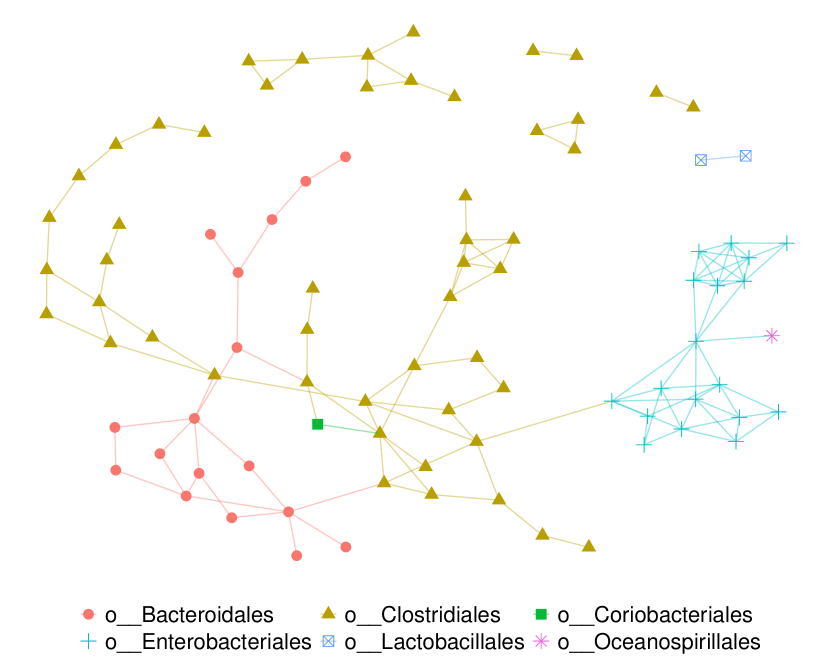
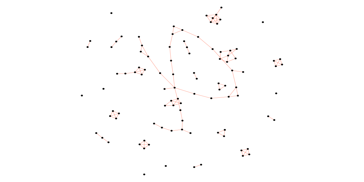
Figure 2: The thAV based on the American Gut Data is shown in Figure 2. To avoid too large graphics, we exclude isolated vertices. The color and the shape of a node imply the biological cluster of each OTU. Figure 2 depicts the thAV applied on the ribloflavin data.

Recovering a Gene Network

In pharmacology, the vitamin riboflavin is industrially produced using diverse microorganisms. Being able to fully understand the bacterias’ genome, biologists promise to further optimize the riboflavin production. The riboflavin data set is provided by the DSM in Switzerland and contains $n=71$ samples and $d=4088$ gen expressions. The R package hdi Dezeure et al. (2015) provides this data set in its implementation. We compare the results of the thAV (see Figure 2) with those of Bühlmann et al. (2014), who analyzed the same data set using a neighborhood regression approach, and observe that the thAV returns a much sparser graph with more cluster-like structures. This does not only increase the interpretability of the graph but also imposes some tight connections between several genes within these clusters.

5 Discussion and Conclusion

Graphical models are a very popular framework for co-occurrence networks, and the graphical lasso is one of the most standard estimators in this framework. In this paper, we generalize the theoretical framework of Chichignoud et al. (2014) for deriving a calibration scheme for the lasso and successfully transfer it to calibrate the graphical lasso. However, our empirical study reveals that graphical lasso estimation itself is not sufficient for effective support recovery, so an additional thresholding step becomes necessary. Our resulting calibration method comes with a finite sample result that allows us to derive a corollary suggesting how to choose a theoretically founded threshold in such a thresholded graphical lasso approach. The resulting estimator, which we call thresholded adaptive validation (thAV) estimator, provides a simple and fast implementation with finite sample guarantees on the recovery performance. To the best of our knowledge, this is the first thresholding methodology for the graphical lasso that comes with a practical, theory-based threshold. Moreover, the thAV clearly outmatches existing graph recovery methods in our empirical analysis, showing both, a high recall but also a high precision in most settings. Other methods, which do not come with a practical threshold, tend to overestimate the graph. Thus, we would recommend the thAV as the method of choice for applications requiring an interpretable and sparse graph structure.

One shortcoming of the proposed procedure is that we replace the tuning parameter $r$ by a quantity $C$, and we even introduce $\lambda$, which defines our threshold. However, regarding $\lambda$, we derive a finite sample result for every $\lambda\in(0,3]$. And secondly, the correspondence between $C$ and the AV regularization parameter leads to a threshold that regulates the impact of $C$ on the thAV, resulting in an estimator that is stable in $C$. In contrast, the calibration via the regularization parameter $r$ is not equipped with such a stability property. The introduction of new hyperparameters can also not be seen as a disadvantage in comparison to related methods, which replace the regularization parameter by other hyperparameters as well. For instance, the StARS calibration scheme for the graphical lasso introduces new parameters $N$ and $b$, which define the number of $N$ subsamples of size $b$, and the parameter $\beta$, which restricts the instability. TIGER introduces a new regularization parameter $\xi$ and the authors Liu and Wang (2017) argue that the final problem is regularization-parameter-insensitive.

On the other hand, a major advantage of this calibration scheme is its generality. While we focus on the graphical lasso in this paper, the derived theoretical framework can also serve as a foundation for other thresholding approaches, which are not limited to Gaussian graphical modeling. For instance, the proposed method has the potential to effectively tune the rSME, which is a graph recovery method for the pairwise interaction model. Using the same primal dual-witness technique, the authors Lin et al. (2016) prove the assumption on which our theoretical framework is based (see (4)). Hence, we can derive the same theory for these types of estimators using the adaptive validation technique. We note that many empirical results regarding the rSME are rather limited to ROC curves, which conceal the regularization parameter selection. Moreover, we can also employ the framework for methods that aim to recover the support of specific types of graph topologies, such as particularly scale-free graphs Liu and Ihler (2011).

For future work, we hope to apply the proposed general framework to calibrate regularized optimization problems and equip these estimators with finite sample theoretical guarantees. These might include other applications of sparse precision matrix estimation such as high-dimensional discriminant analysis and portfolio allocation (see Fan et al. (2016) and references therein), but also applications beyond the scope of sparse precision matrix estimation.

A Supplementary Theory

This section provides theory and proofs that are used in the main paper. First, following the theoretical framework proposed by Chichignoud et al. (2014), we introduce a general calibration scheme for a broad class of regularized optimization problems in Section A.1. Our general framework is based on a central assumption, which we prove for the graphical lasso in Section A.2.

A.1 A General Calibration Scheme for Regularized Optimization

Regularizing an optimization problem has proved to serve as an useful concept in various settings to prevent overfitting (i.e. Tibshirani (1996)), increase numerical stability (i.e. Hoerl and Kennard (2000)), and because there arise attractive properties from a statistical perspective (i.e. Zhuang and Lederer (2018); Wainwright (2019)). Further, various constrained optimization problems can be reframed as regularized unconstrained optimization problems Boyd and Vandenberghe (2009), which are appealing from a computational perspective. However, many of these regularized optimization methods hinge in finding a suitable regularization parameter and hence it became common to fall back on heuristics or asymptotic methods. We generalize the idea in Chichignoud et al. (2014) to obtain a calibration scheme for a general optimization problem. The resulting estimator comes with a finite sample bound on its performance and is computationally cheap as it requires only $1$ solution path.

Consider an optimization problem of the form

$$\hat{\Theta}_{r}\in\operatorname*{\arg\!\min}_{\Omega\in\mathbb{S}}\bigl{\{}f(\boldsymbol{Z},\Omega)+rh(\Omega)\bigr{\}}\enspace,$$ (S1)

where $\mathbb{S}$ is a collection of possible estimators, $r$ is a real-valued regularization parameter, $\boldsymbol{Z}$ is the observed data, $f$ is a function measuring the fit of the estimator $\Omega$ having observed data $\boldsymbol{Z}$, and $h$ is some regularization function depending only on the estimator $\Omega$. The optimization problem usually frames all quantities except of the regularization parameter, which is often tuned based on heuristics or personal intuition. Let us fix a symmetric loss function $\ell:\mathbb{S}\times\mathbb{S}\rightarrow\mathbb{R}^{+}$ that satisfies the triangle inequality. Our goal is then to calibrate $r$ such that we can bound the loss $\ell(\Theta,\hat{\Theta}_{r})$ between the estimation target $\Theta$ and the estimator $\hat{\Theta}_{r}$.

We propose the following generalized version of the AV estimator Chichignoud et al. (2014).

Definition 5 (AV).

Let $\mathcal{R}\subset\mathbb{R}$ be a finite and nonempty set of regularization parameters. Then, the adaptive validation (AV) calibration scheme selects the regularization parameter according to

$$\hat{r}:=\operatorname{min}\bigl{\{}r\in\mathcal{R}:\ell\bigl{(}\hat{\Theta}_{r^{\prime}},\hat{\Theta}_{r^{\prime\prime}}\bigr{)}\leq k(r^{\prime})+k(r^{\prime\prime})\enspace\forall r^{\prime},r^{\prime\prime}\in\mathcal{R}\cap[r,\infty)\bigr{\}}\enspace,$$

where $k:\mathcal{R}\rightarrow\mathbb{R}^{+}$ is a monotonly increasing and positive function (specified in the following) and $\hat{\Theta}_{r^{\prime}},\hat{\Theta}_{r^{\prime\prime}}$ are the estimators (S1) using regularization parameter $r^{\prime}$ and $r^{\prime\prime}$, respectively. We call $\hat{\Theta}_{\hat{r}}$ (resulting from inserting $\hat{r}$ into (S1)) the AV estimator.

In contrast to Chichignoud et al. (2014), our general theory is not restricted to the setting of lasso regression and we modify the definition by incorporating $k$. The definition in Chichignoud et al. (2014) is limited to linear $k$. To allow for a general theory, we defer the restrictions from the specific type of optimization problem (again, (S1) is very general) to the following assumption, on which our theory is based.

Assumption 6.

Let $\bigl{(}\mathcal{T}_{r}\bigr{)}_{r\in\mathcal{R}}$ be a class of events indexed by $r\in\mathcal{R}$. Assume that $\mathcal{T}_{r}$ is monotonly increasing in $r$, that is, $\mathcal{T}_{r^{\prime}}\subset\mathcal{T}_{r^{\prime\prime}}$ for $r^{\prime}\leq r^{\prime\prime}$. Suppose further that, conditioned on $\mathcal{T}_{r}$, it holds

$$\ell\bigl{(}\Theta,\hat{\Theta}_{r}\bigr{)}\leq k(r)\enspace,$$ (S2)

where $\hat{\Theta}_{r}$ is the regularized estimator (S1) and $\Theta$ is the estimation target.

Hence, dependent on the setting at hand, Assumption 6 defines the function $k$ that is used in the AV calibration scheme in Definition 5. By deriving theory for arbitrary positive and monotonly increasing functions $k$, we want to emphasize that we can fit very general frameworks into the setting that is described by Assumption 6 to obtain finite sample results from Theorem 2.

As in the main paper, we can define an optimal regularization parameter by the smallest regularization parameter $r_{\delta}^{\ast}$ that allows us to employ (S2) with probability $1-\delta$ for $\delta\in(0,1]$:

$$r_{\delta}^{\ast}:=\operatorname*{\arg\!\min}_{r\in\mathcal{R}}\left\{\mathbb{P}\bigl{(}\mathcal{T}_{r}\bigr{)}\geq 1-\delta\right\}.$$ (S3)

Since we do not know $\mathbb{P}(\mathcal{T}_{r})$ in practice, we cannot access $r_{\delta}^{\ast}$ and must rely on approximations. The following theorem, which is a generalization of Theorem $3$ by Chichignoud et al. (2014), guarantees that the AV estimator comes with finite sample bounds on the approximation of the estimation target.

Theorem 7 (Finite-Sample Bound for the AV).

Suppose that Assumption 6 holds and that $\hat{r}$ is the regularization parameter selected by the AV method. Then, for any $\delta\in(0,1)$, it holds that

$$\hat{r}\leq r_{\delta}^{\ast}\quad\textrm{ and }\quad\ell\bigl{(}\Theta,\hat{\Theta}_{\hat{r}}\bigr{)}\leq 3k(r_{\delta}^{\ast})$$ (S4)

with probability at least $1-\delta$.

Proof.

Per definition of $r_{\delta}^{\ast}$, we know that $\mathbb{P}\bigl{(}\mathcal{T}_{r_{\delta}^{\ast}}\bigr{)}\geq 1-\delta$, hence, it is sufficient to show that (S4) holds conditioned on $\mathcal{T}_{r_{\delta}^{\ast}}$.
Let

$$\hat{r}:=\operatorname{min}\bigl{\{}r\in\mathcal{R}:\ell\bigl{(}\hat{\Theta}_{r^{\prime}},\hat{\Theta}_{r^{\prime\prime}}\bigr{)}\leq k(r^{\prime})+k(r^{\prime\prime})\enspace\forall r^{\prime},r^{\prime\prime}\in\mathcal{R}\cap[r,\infty)\bigr{\}}\enspace,$$ (S5)

be the AV regularization parameter. Our first goal is to prove that $\hat{r}\leq r_{\delta}^{\ast}$, which we will do by contradiction. For that, assume that $\hat{r}>r_{\delta}^{\ast}$. Then, there must exist $r^{\prime},r^{\prime\prime}\in\mathcal{R}\cap[r_{\delta}^{\ast},\,\infty)$ such that

$$\ell\bigl{(}\hat{\Theta}_{r^{\prime}},\hat{\Theta}_{r^{\prime\prime}}\bigr{)}>k(r^{\prime})+k(r^{\prime\prime})$$ (S6)

because otherwise $\hat{r}$ could not be a minimizer of the set in (S5). Per Assumption, we know that $\mathcal{T}_{r_{\delta}^{\ast}}\subset\mathcal{T}_{r^{\prime}},\mathcal{T}_{r^{\prime\prime}}$ since $r^{\prime},\,r^{\prime\prime}\geq r_{\delta}^{\ast}$. As we condition on $\mathcal{T}_{r_{\delta}^{\ast}}$, we know due to (S2) that

$$\ell\bigl{(}\Theta,\hat{\Theta}_{r^{\prime}}\bigr{)}\leq k(r^{\prime})\quad\text{ and }\quad\ell\bigl{(}\Theta,\hat{\Theta}_{r^{\prime\prime}}\bigr{)}\leq k(r^{\prime\prime})\enspace.$$

Using the triangle inequality, we conclude that

$$\ell\bigl{(}\hat{\Theta}_{r^{\prime}},\hat{\Theta}_{r^{\prime\prime}}\bigr{)}\leq\ell\bigl{(}\hat{\Theta}_{r^{\prime}},\Theta\bigr{)}+\ell\bigl{(}\Theta,\hat{\Theta}_{r^{\prime\prime}}\bigr{)}\leq k(r^{\prime})+k(r^{\prime\prime})\enspace.$$

However, this contradicts (S6). Consequently, it must hold that $\hat{r}\leq r_{\delta}^{\ast}$.
To prove the loss bound in (S4), we observe that it is $\hat{r},r_{\delta}^{\ast}\in\mathcal{R}\cap[\hat{r},\infty)$ as previously shown. Therefore, we know per definition of the AV regularization parameter $\hat{r}$ that

$$\ell\bigl{(}\hat{\Theta}_{\hat{r}},\hat{\Theta}_{r_{\delta}^{\ast}}\bigr{)}\leq k(\hat{r})+k(r_{\delta}^{\ast})\enspace.$$ (S7)

Finally, using the triangle inequality once more, we find

$$\ell\bigl{(}\Theta,\hat{\Theta}_{\hat{r}}\bigr{)} \leq\ell\bigl{(}\Theta,\hat{\Theta}_{r_{\delta}^{\ast}}\bigr{)}+\ell\bigl{(}\hat{\Theta}_{\hat{r}},\hat{\Theta}_{r_{\delta}^{\ast}}\bigr{)}$$

$$\leq k(r_{\delta}^{\ast})+k(\hat{r})+k(r_{\delta}^{\ast})$$

$$\leq 3k(r_{\delta}^{\ast})\enspace,$$

where we used (S7) in the second inequality and $\hat{r}\leq r_{\delta}^{\ast}$ and the monotonicity of $k$ in the third inequality. ∎

In summary, the AV calibration scheme as defined in Definition 5 is a calibration scheme for very general optimization problems (S1). We impose almost no restrictions on the optimization problem (S1) itself but defer the restrictions to Assumption 6. But once we can prove (S2), which is of a very general form, we are immediately able to obtain finite sample results as stated in Theorem 7.

A.2 Adaptive Validation for the Graphical Lasso

In this section, we apply the proposed calibration scheme from the previous section to calibrate the graphical lasso regularization parameter. Importantly, we substantiate the validity of Assumption 6 and thus obtain the finite sample results for the AV graphical lasso estimator (see Theorem $2$ from the main paper).

Recall, the graphical lasso optimization problem is defined as

$$\hat{\Theta}_{r}=\operatorname*{\arg\!\min}_{\Omega\in\operatorname*{\mathcal{S}_{d}^{+}}+}\biggl{\{}\operatorname{tr}\biggl{[}\frac{1}{n}\sum_{i=1}^{n}\bigl{(}\boldsymbol{z}^{(i)}\bigr{)}^{\top}\boldsymbol{z}^{(i)}\Omega\biggr{]}-\log\left[\det\left[\Omega\right]\right]+r\|\Omega\|_{1,\operatorname{off}}\biggr{\}}\enspace.$$ (S8)

Plainly, the graphical lasso optimization problem fits into the general setting in (S1).

It remains to prove that Assumption 6 is valid. In the following, we consider

$$k(r):=Cr\enspace\text{ and }\enspace\ell(\Theta^{\prime},\Theta^{\prime\prime}):=\max_{\begin{subarray}{c}i,j\in\mathcal{V}\\ i\neq j\end{subarray}}|\Theta_{ij}^{\prime}-\Theta_{ij}^{\prime\prime}|\enspace$$

for some constant $C>0$. Hence, we aim to prove the existence of a monotone increasing class $(\mathcal{T}_{r})_{r\in\mathcal{R}}$ such that, conditioned on $\mathcal{T}_{r}$, it holds

$$\ell\bigl{(}\Theta,\hat{\Theta}_{r}\bigr{)}\leq Cr\enspace,$$ (S9)

where $\hat{\Theta}_{r}$ is the graphical lasso, $\Theta$ is the true precision matrix, and $C$ is a constant.

We make use of the extensive investigations by Ravikumar et al. (2011) to derive the validity of this assumption. Our result (Theorem 12), which states a $\ell$-bound as in (S9), follows similar steps as those in the proof of Theorem 1 by Ravikumar et al. (2011):

Required Definitions

In order to obtain a result that substantiates (S9), it is necessary to impose the estimation target $\Theta$ to be well-behaved. In the following we introduce some quantities that allow us to define such a well behaviour of $\Theta$. As we will see, the Hessian of the mapping

$$g:\operatorname*{\mathcal{S}_{d}^{+}}+\rightarrow\mathbb{R},\;\Omega\mapsto\log(\det[\Omega])$$

at $\Theta$, which we define as

$$\Gamma:=\frac{\partial^{2}g(\Theta)}{\partial\Omega^{2}}\Bigg{|}_{\Omega=\Theta}\enspace$$

plays a central role in describing a well behaviour of the precision matrix. We index $\Gamma$ by vertex pairs

$$\Gamma_{(j,k),(l,m)}=\frac{\partial^{2}g(\Theta)}{\partial\Omega_{jk}\partial\Omega_{lm}}\Bigg{|}_{\Omega=\Theta}\enspace,$$ (S10)

where $(j,k),(l,m)\in\mathcal{V}\times\mathcal{V}$. Further, let $S:=\mathcal{E}\cup\{(i,i):\,i\in\mathcal{V}\}$ be the edge set of the graphical model including the self-directed edges. Then, according to the indexation in (S10), we can define the quantities

$$\Gamma_{SS}:=\bigl{(}\Gamma_{(j,k),(l,m)}\bigr{)}_{(j,k),(l,m)\in S}\enspace\text{ and }\enspace\Gamma_{eS}:=\bigl{(}\Gamma_{e,(l,m)}\bigr{)}_{(l,m)\in S}\enspace\forall e\in S\enspace.$$

Finally, we define

$$\kappa_{\Sigma}:={\left|\kern-1.07639pt\left|\kern-1.07639pt\left|\Sigma\right|\kern-1.07639pt\right|\kern-1.07639pt\right|}_{\infty}\enspace\text{ and }\enspace\kappa_{\Gamma}:={\left|\kern-1.07639pt\left|\kern-1.07639pt\left|(\Gamma_{SS})^{-1}\right|\kern-1.07639pt\right|\kern-1.07639pt\right|}_{\infty}\enspace,$$

where ${\left|\kern-1.07639pt\left|\kern-1.07639pt\left|\cdot\right|\kern-1.07639pt\right|\kern-1.07639pt\right|}_{\infty}$ defines the $\ell_{\infty}$-operator norm, that is,

$${\left|\kern-1.07639pt\left|\kern-1.07639pt\left|\Sigma\right|\kern-1.07639pt\right|\kern-1.07639pt\right|}_{\infty}:=\max_{i=1,...d}\sum_{j=1}^{d}|\Sigma_{ij}|\enspace.$$

In the following paragraph, we use these quantities to describe conditions under which the so called Primal-Dual Witness Construction (PDW) succeeds. The idea of PDW is based on the primal solution $\tilde{\Theta}_{r}$, which is the solution of the graphical lasso that is constrained on the true edge set. Hence, this is the solution of the following graphical lasso optimization problem

$$\tilde{\Theta}_{r}:=\operatorname*{\arg\!\min}_{\Omega\in\operatorname*{\mathcal{S}_{d}^{+}}+,\Omega_{S^{\complement}}=0}\bigg{\{}\operatorname{tr}\biggl{[}\frac{1}{n}\sum_{i=1}^{n}\bigl{(}\boldsymbol{z}^{(i)}\bigr{)}^{\top}\boldsymbol{z}^{(i)}\Omega\biggr{]}-\log\bigl{[}\det[\Omega]\bigr{]}+r\|\Omega\|_{1,\operatorname{off}}\bigg{\}}\enspace,$$

where $S^{\complement}:=\{(i,j)\in\mathcal{V}\times\mathcal{V}:\;(i,j)\not\in\mathcal{E}\}$ and $\Omega_{S^{\complement}}$ are the components $\Omega_{ij}$ such that $(i,j)\in S^{\complement}$. As $S$ is unknown in practice, this construction is only relevant from a technical perspective. We say that the PDW succeeds if the unconstrained graphical lasso $\hat{\Theta}_{r}$ equals the primal solution $\tilde{\Theta}_{r}$.

Incoherence and bounded norm of the Primal

Now we are ready to impose a well behaviour on $\Theta$ that ensures the PDW to succeed and which eventually implies the validity of (S9), see Theorem 12.

Assumption 8 ($\Theta$ well-behaved).

There exists an $\alpha\in(0,1]$ such that

1. $\max_{e\in S^{\complement}}\|\Gamma_{eS}\bigl{(}\Gamma_{SS}\bigr{)}^{-1}\|_{1}\leq 1-\alpha\quad$,

2. $\ell_{\infty}\bigl{(}\Theta,\tilde{\Theta}_{r}\bigr{)}\leq\bigl{(}3\kappa_{\Sigma}\operatorname{deg}(\Theta)\bigr{)}^{-1}\text{ for all }r\in\mathcal{R},$ where $\ell_{\infty}(\Theta^{\prime},\Theta^{\prime\prime}):=\max_{i,j\in\mathcal{V}}|\Theta_{ij}^{\prime}-\Theta_{ij}^{\prime\prime}|$ and $\operatorname{deg}(\Theta)$ denotes the maximum degree of the corresponding conditional dependency graph induced by $\Theta$.

The first assumption is widely used and is often referred to as incoherence or irrepresentability condition. To shed some light onto this condition Ravikumar et al. (2011) consider for $i,j\in\mathcal{V}$ the centered random variable $y_{ij}:=z_{i}z_{j}-\mathbb{E}[z_{i}z_{j}]$, which can be interpreted as the interaction between components $z_{i}\text{ and }z_{j}$. One can show that the incoherence condition requires $y_{ij}$ for $(i,j)\not\in\mathcal{E}$ to be not highly correlated with $y_{lm}$ with $(l,m)\in\mathcal{E}$. Hence, the incoherence assumption bounds the correlation between irrelevant interactions, $y_{ij}$ with $(i,j)\not\in\mathcal{E}$, and relevant interactions, $y_{ij}$ with $(i,j)\in\mathcal{E}$. This interpretation goes in line with the incoherence condition for the lasso, see Ravikumar et al. (2011) and references therein for further details.
The second assumption states that the constrained graphical lasso $\tilde{\Theta}_{r}$, i.e. the primal solution, is accurate enough in the sense that it satisfies the $\ell_{\infty}$-bound. Note, that the bound scales with the maximal degree of the graph. Hence, the higher the degree of the true graph, the more accurate the primal solution must be to satisfy Assumption 8. This indicates a reason why scale-free graphs, which have in general a larger maximal degree than random graphs, tend to be harder to be well-estimated by the graphical lasso.

In the following we consider $n$ samples $\boldsymbol{z}^{(1)},\dots,\boldsymbol{z}^{(n)}$ drawn independently from $\boldsymbol{z}\sim\mathcal{N}_{d}(\boldsymbol{0}_{d},\Sigma)$ for a positive definite covariance matrix $\Sigma$. Along the line of thoughts of Ravikumar et al. (2011), we can make use of Assumption 8 and obtain the following theoretical properties. We start by stating conditions for a $\ell_{\infty}$-bound of the primal solution $\tilde{\Theta}_{r}$ (Lemma 9). Next, we state conditions, under which it holds that $\hat{\Theta}_{r}=\tilde{\Theta}_{r}$ (Lemma 10), so that Lemma 9 gives us a $\ell_{\infty}$-bound for the graphical lasso $\hat{\Theta}_{r}$. Finally, we use another Lemma (Lemma 11) to show that the conditions in Lemma 10 are satisfied. The proofs of Lemma 9, 10, and 11 can be found in Ravikumar et al. (2011).

Lemma 9 (Lemma $6$ in Ravikumar et al. (2011)).

Assume that

$$2\kappa_{\Sigma}\bigl{(}\ell_{\infty}\bigl{(}\Sigma,\,\hat{\Sigma}_{\operatorname{emp}}\bigr{)}+r\bigr{)}\leq C^{\prime}\enspace,$$ (S11)

where $C^{\prime}:=\min\bigl{\{}(3\kappa_{\Gamma}\operatorname{deg}(\Theta))^{-1},\,(3\kappa^{3}_{\Sigma}\kappa_{\Gamma}\operatorname{deg}(\Theta))^{-1}\bigr{\}}$, and $\hat{\Sigma}_{\operatorname{emp}}:=1/n\sum_{i=1}^{n}(\boldsymbol{z}^{(i)})^{\top}\boldsymbol{z}^{(i)}$ is the empirical covariance matrix. Then it holds that

$$\ell_{\infty}\bigl{(}\Theta,\,\tilde{\Theta}_{r},\bigr{)}\leq 2\kappa_{\Sigma}\bigl{(}\ell_{\infty}\bigl{(}\Sigma,\,\hat{\Sigma}_{\operatorname{emp}}\bigr{)}+r\bigr{)}\enspace.$$ (S12)

Lemma 10 (Lemma $3$ $+$ Lemma $4$ in Ravikumar et al. (2011)).

Suppose that

$$\operatorname{max}\bigl{\{}\ell_{\infty}\bigl{(}\Sigma,\,\hat{\Sigma}_{\operatorname{emp}}\bigr{)},\;\|R\|_{\infty}\bigr{\}}\leq\frac{\alpha r}{8}\enspace,$$

where

$$R:=\tilde{\Theta}_{r}^{-1}-\Theta^{-1}+\Theta^{-1}\bigl{(}\tilde{\Theta}_{r}-\Theta\bigr{)}\Theta^{-1}\enspace$$

is the remainder of the first-order Taylor approximation of $\tilde{\Theta}_{r}^{-1}$ at $\Theta$. Then it holds that $\tilde{\Theta}_{r}=\hat{\Theta}_{r}$.

Lemma 11 (Lemma 5 in Ravikumar et al. (2011)).

Suppose that part 2 in Assumption 8 is satisfied. Then, it holds that

$$\|R\|_{\infty}\leq\frac{\kappa_{\Sigma}}{6\operatorname{deg}(\Theta)}\enspace.$$ (S13)

Bound for the graphical lasso

Having introduced this bunch of lemmas, we are ready to put the pieces together and obtain the following theorem that summarizes the aforementioned lemmas and assumptions, and that proves the validity of (S9).

Theorem 12 ($\ell$-Bound for the Graphical Lasso).

Suppose that Assumption 8 holds. Then, conditioned on

$$\mathcal{T}_{r}:=\Biggl{\{}\max\Bigl{\{}\ell_{\infty}\bigl{(}\Sigma,\,\hat{\Sigma}_{\operatorname{emp}}\bigr{)},\frac{\kappa_{\Sigma}}{6\operatorname{deg}(\Theta)}\Bigr{\}}\leq\frac{\alpha r}{8}\Biggr{\}}\ ,$$ (S14)

it holds for $r\leq\frac{4}{\kappa_{\Sigma}(\alpha+8)}C^{\prime}$ that

$$\ell(\Theta,\,\hat{\Theta}_{r})\leq\kappa_{\Gamma}\frac{\alpha+8}{4}r\enspace.$$

Proof.

First, note that conditioned on $\mathcal{T}_{r}$, we almost satisfy the conditions in Lemma 10. It remains to show that $\|R\|_{\infty}\leq\alpha r/8$. However, this is true since

$$\|R\|_{\infty}\leq\frac{\kappa_{\Sigma}}{6\operatorname{deg}(\Theta)}\leq\frac{\alpha r}{8},$$

where the first inequality follows from Lemma 11, and the second inequality follows from the condition on $\mathcal{T}_{r}$. Therefore, the primal-dual construction succeeds (Lemma 10), that is, $\tilde{\Theta}_{r}=\hat{\Theta}_{r}$. Thus, we obtain a $\ell_{\infty}$-bound for the graphical lasso (S12), if (S11) in Lemma 9 is satisfied. Plugging in our assumptions, we see that this is indeed the case, since

$$2\kappa_{\Sigma}\bigl{(}\ell_{\infty}\bigl{(}\Sigma,\,\hat{\Sigma}_{\operatorname{emp}}\bigr{)}+r\bigr{)} \leq 2\kappa_{\Sigma}\bigl{(}\frac{\alpha r}{8}+r\bigr{)}$$

$$=2\kappa_{\Sigma}\frac{\alpha+8}{8}r$$

$$\leq 2\kappa_{\Sigma}\frac{\alpha+8}{8}\frac{4}{\kappa_{\Sigma}(\alpha+8)}C^{\prime}$$

$$=C^{\prime}\enspace.$$

Hence, we obtain

$$\ell(\Theta,\hat{\Theta}_{r})\leq\ell_{\infty}\bigl{(}\Theta,\hat{\Theta}_{r}\bigr{)}=\ell_{\infty}\bigl{(}\Theta,\tilde{\Theta}_{r}\bigr{)}\leq\kappa_{\Sigma}\frac{\alpha+8}{4}r\enspace.$$

∎

Theorem 12 is very similar to Theorem 1 by Ravikumar et al. (2011), but differs in $2$ important aspects:

1. Ravikumar et al. (2011) fix a regularization parameter (dependent on $\alpha$, the amount of samples $n$, and some quantity $q$). On the other hand, Theorem 12 is a bound for a range of regularization parameters;

2. Ravikumar et al. (2011) derive a probabilistic bound (where the probability that this bound holds is determined by $q$). Theorem 12 is, conditioned on a class of events $\mathcal{T}_{r}$, a deterministic bound.

The purpose of these changes is to fit the result to our setting that is generalized by Assumption 6.

Note that $\mathcal{T}_{r}$ in Theorem 12 bounds two quantities, whereas the first one describes an effective noise in the empirical covariance matrix. Therewith, it shares the same intuition as the set considered for the linear regression problem in Chichignoud et al. (2014): the larger the noise, the larger we need to choose the regularization parameter to be able to control these fluctuations. Consequently, the set of “controllable” scenarios $\mathcal{T}_{r}$ grows with $r$. On the other hand, large noise shrinks the set of these scenarios. Even though we obtain a class of events $\bigl{(}\mathcal{T}_{r}\bigr{)}_{r\in\mathcal{R}}$ sharing a similar interpretation to the class considered in Chichignoud et al. (2014), we have to resort to a more involved primal-dual-witness construction to get these results. Further, we need to keep in mind that Theorem 12 supposes $r\leq 4/(\kappa_{\Sigma}(\alpha+8))C^{\prime}$, which means that the set of possible regularization parameters $\mathcal{R}$ must satisfy $\mathcal{R}\subset(0,4/(\kappa_{\Sigma}(\alpha+8))C^{\prime}]$.

Lastly, although the primal-dual witness construction underpinning Theorem 12 already implies that there are no false positives, we show robustness against false positives independently for our calibration scheme in Corollary $4$ in the main paper. This way, we make the theory we are presenting less dependent on the specific assumptions of Theorem 12.

A.3 Remaining Proofs of the Results in the Main Paper

Proof of Corollary $4$

Based on Theorem 7, we derive Corollary $4$ from the main text, which provides strong graph recovery results for the thAV. In the following we write $\hat{\Theta}:=\hat{\Theta}_{r}$ to enhance readability.

Proof.

The first statement is a direct consequence of Theorem 7 applied to this setting: Consider any zero-entry $\Theta_{ij}=0$ of the precision matrix. Therefore, (S4) yields with probability $1-\delta$ that

$$|\hat{\Theta}_{ij}|=|\Theta_{ij}-\hat{\Theta}_{ij}|\leq 3Cr_{\delta}^{\ast}\quad\text{and}\quad\hat{r}\leq r_{\delta}^{\ast}\enspace.$$

Hence, it holds with probability $1-\delta$ that $|\hat{\Theta}_{ij}|\in[0,\,3Cr_{\delta}^{\ast}]$ and that $\lambda C\hat{r}\leq 3C\hat{r}\leq 3Cr_{\delta}^{\ast}$, which we need to prove the well-definedness of the interval $(\lambda C\hat{r},\,3Cr_{\delta}^{\ast}$]. This proves part $1$.
To prove 2., let us consider a significant edge $(i,j)$ such that $|\Theta_{ij}|>(3+\lambda)Cr_{\delta}^{\ast}$. We prove the result via contradiction. Hence, let us assume that $\hat{\Theta}_{ij}^{t}=0$. It follows that $|\hat{\Theta}_{ij}|<\lambda C\hat{r}\leq\lambda Cr_{\delta}^{\ast}$ with probability $1-\delta$, where the first inequality follows via the definition and the second inequality follows via Theorem 7. But then, using the reversed triangle inequality, it holds that

$$|\Theta_{ij}-\hat{\Theta}_{ij}|\geq|\Theta_{ij}|-|\hat{\Theta}_{ij}|>(3+\lambda)Cr_{\delta}^{\ast}-\lambda Cr_{\delta}^{\ast}=3Cr_{\delta}^{\ast}\enspace,$$

which contradicts (S4). Hence, $\hat{\Theta}^{t}_{ij}$ cannot be zero-valued and therefore it is $(i,j)\in\hat{\mathcal{E}}$. ∎

Behaviour of $\hat{r}$ in $C$

The proposed AV calibration scheme employs a hyperparameter $C$ that is related to our central Assumption 6. For completeness, we prove that the AV regularization parameter $\hat{r}$ is decreasing in $C$.

Proposition 13.

Consider the AV regularization parameter $\hat{r}_{C}$ as a quantity of $C$. Then, $\hat{r}_{C}$ is monotonely decreasing in $C$.

Proof.

Consider any $C>0$. Then, according to the definition of $\hat{r}_{C}$, it holds for any positive $r^{\prime},r^{\prime\prime}\in\mathcal{R}\text{ with }\hat{r}_{C}\leq r^{\prime},r^{\prime\prime}$ that

$$\frac{\ell\bigl{(}\hat{\Theta}_{r^{\prime}},\,\hat{\Theta}_{r^{\prime\prime}}\bigr{)}}{r^{\prime}+r^{\prime\prime}}\leq C\enspace.$$

Therefore, it holds for any $\varepsilon>0$ that

$$\ell\bigl{(}\hat{\Theta}_{r^{\prime}},\,\hat{\Theta}_{r^{\prime\prime}}\bigr{)}\leq C(r^{\prime}+r^{\prime\prime})\leq(C+\varepsilon)(r^{\prime}+r^{\prime\prime})\enspace.$$

This holds for any $r^{\prime},r^{\prime\prime}\geq\hat{r}_{C}$, hence,

$$\hat{r}_{C}\in\Bigl{\{}r\in\mathcal{R}:\ell\bigl{(}\hat{\Theta}_{r^{\prime}},\hat{\Theta}_{r^{\prime\prime}}\bigr{)}\leq(C+\varepsilon)(r^{\prime}+r^{\prime\prime})\enspace\forall r^{\prime},r^{\prime\prime}\in\mathcal{R}\cap[r,\infty)\Bigr{\}}\enspace.$$

Thus, $\hat{r}_{C}$ must be greater than or equal to the minimizer of the above set, which is per definition minimized by $\hat{r}_{C+\varepsilon}$. We conclude that $\hat{r}_{C}\geq\hat{r}_{C+\varepsilon}$ for any $\varepsilon>0$. Since we chose $C>0$ arbitrary, this proves the claim. ∎

B Computational Efficiency of the thAV

In addition to its theoretical finite sample guarantees, the thAV estimator also comes with notable computational benefits. In the following, we consider the thAV technique applied to the graphical lasso optimization problem. In comparison to calibration schemes that are based on data splitting and resampling methods like StARS or other CV-like approaches, thAV only requires at most one solution path $(\hat{\Theta}_{r})_{r\in\mathcal{R}}$. We can readily implement the thAV using Algorithm 1. We observe that using Algorithm 1, we

1. calculate at most $1$ graphical lasso path since we can store and reuse every graphical lasso solution;

2. start to calculate graphical lasso solutions for large regularization parameters and decrease the regularization until we break. Therefore, we most likely avoid to calculate and store graphical lasso solutions for very small regularization parameters, which are computationally most demanding;

3. can use warm starts, which are implemented in the glasso R package Friedman et al. (2008); Witten et al. (2011), to calculate $\hat{\Theta}_{r}$. This decreases the computation time even more.

An implementation of the thAV is provided along with the submission.

Empirically, we can observe that the thAV estimator scales very well in runtime, computational stability, and memory usage even in very large settings. This is an important advantage of thAV in practical applications.

Data: data $Z$, set of increasing regularization parameters $\mathcal{R}$, constant $C$, threshold parameter $\lambda$

Result: thAV estimator

$j\leftarrow\text{length}(\mathcal{R})-1$,       $r\leftarrow\mathcal{R}[j]$,      $\hat{r}\leftarrow\mathcal{R}[1]$

while $r>\mathcal{R}[1]$ do

       $\hat{\Theta}_{r}\leftarrow$ graphical lasso using regularization parameter $r$

       $j^{\prime}\leftarrow\text{length}(\mathcal{R})$,       $r^{\prime}\leftarrow\mathcal{R}[j^{\prime}]$

       while $r^{\prime}>r$ do

             if $\ell(\hat{\Theta}_{r},\;\hat{\Theta}_{r^{\prime}})>C(r+r^{\prime})$ then

                   $\hat{r}\leftarrow\mathcal{R}[j+1]$ // proposed regularization parameter

                   BREAK

                  

            else

                   $j^{\prime}\leftarrow j^{\prime}-1$

                   $r^{\prime}\leftarrow\mathcal{R}[j^{\prime}]$ // decrease until break or $r^{\prime}=r$

                  

            

      $j\leftarrow j-1$

       $r\leftarrow\mathcal{R}[j]$ // decrease until break or $r=\mathcal{R}[1]$

      

AV $\leftarrow\hat{\Theta}_{\hat{r}}$

$t\leftarrow\lambda C\hat{r}$

return AV thresholded by $t=\lambda C\hat{r}$

Algorithm 1 Thresholded adaptive validation graphical lasso

C Experimental Analysis: Details and Additional Experiments

In this section, we present details and additional results of our empirical analysis of the proposed calibration scheme. We describe the methods that are used to generate the precision matrices in Section C.1 and give details about the computation of the estimators that are used for comparison in Section C.2. We extend the empirical analysis from the main paper in Section C.3. In Section C.4 we apply the AV calibration scheme to tune the rSME and a modified version of the graphical lasso that employs power law regularization.

C.1 Precision Generation Methods

This section serves as a detailed description of the generation process of the precision matrices that are used in the experimental analysis. The precision matrices are generated according to the following steps:

• random graph: First, we generate a Gilbert graph Gilbert (1959), that is, we independently connect two nodes $i\neq j$ with some fixed probability $p$, where we choose $p=3/d$ as the default value. Then, we set the non-zero pattern of $\Theta$ according to the adjacency matrix of the Gilbert graph. The next step is to assign all non-zero entries of the precision matrix a value. For each edge $(i,j)$, we sample a value for $\Theta_{ij}=\Theta_{ji}$ from a uniform distribution over the set $I:=[-0.9,\,-0.5]\cup[0.5,\,0.9]$. To guarantee positive definiteness, we set the diagonal entries to $\mu:=-\lfloor\lambda_{\operatorname{min}}(\Theta)\rfloor_{1}$, which is the smallest eigenvalue of $\Theta$ rounded downwards to $1$ decimal place. Finally, we scale $\Theta$ such that it has unit diagonal entries.

• scale-free graph: In this case, the adjacency matrix is generated according to a Barabasi-Albert Algorithm Barabasi (2016) that generates the corresponding graph gradually. The algorithm starts with $2$ connected nodes and adds sequentially a node that will be connected with one of the existent nodes in the network. The probability to be connected to a node $i$ is proportional to its degree, that is,

  $$\mathbb{P}(\{\text{new node connected with node }i\})=\frac{\operatorname{deg}(i)}{\sum_{j\in\mathcal{V}}\operatorname{deg}(j)},$$

  where $\operatorname{deg}(i),\,\operatorname{deg}(j)$ denote the degree of the nodes $i$ and $j$ respectively. We repeat this step until we end up with a graph with $d$ nodes. We set the non-zero pattern of $\Theta$ according to the generated graph and proceed as in the previous case.

Both generation methods are summarized in Algorithm 2.

Data: dimension $d$, type of graph $\operatorname{type}$

Result: positive definite precision matrix

if $\operatorname{type}==\text{random}$ then

       adj $\leftarrow$ adjacency matrix of a Gilbert graph // using the huge package

      

else

       adj $\leftarrow$ adjacency matrix of a scale-free graph // using the huge package

for $i<j\And i,j\in\{1,\dots,d\}$  do

       $\Theta[i,j]\leftarrow\Theta[j,i]\leftarrow$ Sample from a uniform distribution over $[-0.9,\,-0.5]\cup[0.5,\,0.9]$

      

$\operatorname{min.ev}\leftarrow\lfloor\lambda_{\operatorname{min}}(\Theta)\rfloor$ // smallest Eigenvalue of $\Theta$ downwards rounded to $1$ decimal place

$\Theta\leftarrow\Theta+\operatorname{min.ev}\ast I_{d\times d}$

$\Theta\leftarrow 1/\operatorname{min.ev}\ast\Theta$

return Precision matrix $\Theta$ of type $\operatorname{type}$

Algorithm 2 Precision matrix generation

We use pre-implemented functions provided by the R package huge Zhao et al. (2012) to generate the adjacency matrices. The generation of both types of precision matrices is implemented in our attached code. Figure S1 shows an example of both graph structures.

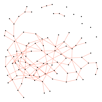
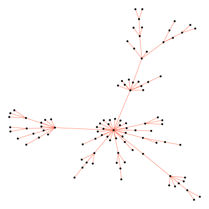
Figure S1: An example of the $2$ graph types that are used in our simulations. Both graphs have $d=100$ nodes. Graph (a) represents a random graph with $p=3/100$, and graph (b) is a scale-free graph according to the described Barabasi-Albert Algorithm.

Precision matrices generated by these methods include values $\Theta_{ij}$ that can be either positive or negative, and vary in absolute value. The absolute values of the generated scale-free graphs tend to be smaller than those of the generated random graphs, which is demonstrated in Figure S2.

C.2 Computational Details

For computing the graphical lasso calibrated via StARS and for computing the TIGER, we employ the R package huge Zhao et al. (2012). As suggested by Liu and Wang (2017), we set the regularization parameter for the TIGER to $\xi=\sqrt{2}/\pi$. The scaled lasso estimator is calculated using the R package scalreg Sun (2019). To obtain the rSME and the SCIO, we employ the genscore package Yu et al. (2019) and the scio package Liu and Luo (2015), respectively. An implementation of the sf-glasso is provided with our submission, which is computed using a reweighted $\ell_{1}$-method proposed by Liu and Ihler (2011). We use $C=0.5$ and $\lambda=2$ to calibrate the rSME, and $C=1.5$ and $\lambda=1.5$ to calibrate the sf-glasso using thAV. If not stated differently, we kept all the default settings.

C.3 Additional Experiments

We evaluate the graph recovery performance based on the $F_{1}$-score, the precision, and the recall of the estimator. These quantities are defined as follows:

$$\textrm{precision}\bigl{(}\mathcal{E},\,\hat{\mathcal{E}}\bigr{)} :=\frac{|\hat{\mathcal{E}}\cap\mathcal{E}|}{|\hat{\mathcal{E}}|}\in[0,1],$$

$$\textrm{recall}\bigl{(}\mathcal{E},\,\hat{\mathcal{E}}\bigr{)} :=\frac{|\hat{\mathcal{E}}\cap\mathcal{E}|}{|\mathcal{E}|}\in[0,1],$$

where $\mathcal{E},\;\hat{\mathcal{E}}$ are the edge sets obtained from the non-zero patterns of $\Theta$ and some estimate $\hat{\Theta}$, respectively. While precision and recall behave very similar to the number of false positives and the number of false negatives, respectively, they also put the size of the edge sets into relation. The $F_{1}$-score puts both measures, precision and recall, into relation

$$F_{1}\bigl{(}\mathcal{E},\,\hat{\mathcal{E}}\bigr{)} :=\Biggl{(}\frac{\operatorname{precision}\bigl{(}\mathcal{E},\,\hat{\mathcal{E}}\bigr{)}^{-1}+\operatorname{recall}\bigl{(}\mathcal{E},\,\hat{\mathcal{E}}\bigr{)}^{-1}}{2}\Biggr{)}^{-1}\in[0,1].$$

In the best case, where we correctly assign all edges, that is, if $\hat{\mathcal{E}}=\mathcal{E}$, we get a $F_{1}$-score equal to $1$. The worst $F_{1}$-score is $0$, if either precision or recall is equal to $0$.

In the following, we complement the simulation study from the main text. Similar to the main paper, we average the experiments over $25$ iterations (if not stated differently) and standard deviations are presented in parenthesis.

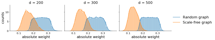
Figure S2: Histograms of the absolute valued non-zero weights $|\Theta_{ij}|$ of $50$ scale-free and $50$ random graphs generated by the procedure described in Section C.1. We considered graphs with $d\in\{200,300,500\}$ nodes.

Table 1: Graph recovery performance for varying graphs and sample size. The bold numbers indicate the best score in each setting.

		random				scale-free
		$F_{1}$	Precision	Recall		$F_{1}$	Precision	Recall
$n=300,\,d=100$
oracle		0.67 (0.11)	0.55 (0.14)	0.88 (0.06)		0.41 (0.11)	0.46 (0.28)	0.67 (0.30)
StARS		0.57 (0.12)	0.42 (0.10)	0.91 (0.07)		0.32 (0.11)	0.21 (0.09)	0.75 (0.10)
scaled lasso		0.70 (0.03)	0.54 (0.03)	0.99 (0.01)		0.48 (0.04)	0.32 (0.04)	$\boldsymbol{0.97}$ (0.03)
TIGER		0.54 (0.08)	0.37 (0.08)	0.98 (0.01)		0.40 (0.07)	0.25 (0.06)	$\boldsymbol{0.97}$ (0.03)
rSME (eBIC)		0.41 (0.17)	0.27 (0.13)	$\boldsymbol{1.00}$ (0.00)		0.37 (0.18)	0.24 (0.13)	0.96 (0.04)
scio (CV)		0.46 (0.45)	0.46 (0.45)	0.46 (0.46)		0.25 (0.29)	0.45 (0.48)	0.19 (0.24)
scio (Bregman)		0.19 (0.08)	0.13 (0.15)	0.98 (0.11)		0.31 (0.23)	0.34 (0.32)	0.77 (0.28)
thAV		$\boldsymbol{0.90}$ (0.06)	$\boldsymbol{0.87}$ (0.08)	0.93 (0.05)		$\boldsymbol{0.66}$ (0.10)	$\boldsymbol{0.53}$ (0.13)	0.91 (0.05)
$n=200,\,d=200$
oracle		0.69 (0.11)	0.61 (0.16)	0.83 (0.03)		0.35 (0.08)	0.34 (0.19)	0.54 (0.19)
StARS		0.56 (0.11)	0.41 (0.11)	0.93 (0.03)		0.30 (0.08)	0.20 (0.07)	0.62 (0.11)
scaled lasso		0.66 (0.03)	0.50 (0.03)	0.96 (0.02)		0.37 (0.05)	0.25 (0.04)	0.71 (0.09)
TIGER		0.48 (0.08)	0.32 (0.07)	$\boldsymbol{0.97}$ (0.01)		0.32 (0.07)	0.20 (0.06)	$\boldsymbol{0.76}$ (0.09)
rSME (eBIC)		0.60 (0.30)	0.51 (0.27)	0.90 (0.19)		$\boldsymbol{0.43}$ (0.17)	0.48 (0.23)	0.55 (0.19)
scio (CV)		0.12 (0.25)	0.22 (0.41)	0.09 (0.21)		0.04 (0.10)	0.16 (0.37)	0.03 (0.06)
scio (Bregman)		0.45 (0.28)	0.43 (0.36)	0.87 (0.18)		0.37 (0.12)	$\boldsymbol{0.87}$ (0.08)	0.26 (0.14)
thAV		$\boldsymbol{0.84}$ (0.07)	$\boldsymbol{0.79}$ (0.12)	0.91 (0.06)		0.39 (0.15)	0.31 (0.19)	0.69 (0.10)
$n=300,\,d=300$
oracle		0.76 (0.10)	0.69 (0.14)	0.87 (0.03)		0.30 (0.08)	0.29 (0.24)	0.60 (0.20)
StARS		0.61 (0.09)	0.45 (0.10)	0.96 (0.03)		0.23 (0.09)	0.15 (0.07)	0.56 (0.10)
scaled lasso		0.68 (0.02)	0.52 (0.02)	0.98 (0.01)		0.34 (0.05)	0.22 (0.03)	0.73 (0.09)
TIGER		0.44 (0.10)	0.29 (0.08)	$\boldsymbol{0.99}$ (0.01)		0.27 (0.07)	0.17 (0.06)	$\boldsymbol{0.78}$ (0.11)
rSME (eBIC)		0.72 (0.11)	0.58 (0.13)	0.97 (0.02)		0.32 (0.21)	0.32 (0.23)	0.63 (0.23)
scio (CV)		0.25 (0.39)	0.35 (0.47)	0.23 (0.36)		0.09 (0.13)	0.36 (0.49)	0.05 (0.07)
scio (Bregman)		0.38 (0.33)	0.31 (0.33)	0.98 (0.05)		0.30 (0.06)	$\boldsymbol{0.92}$ (0.09)	0.18 (0.04)
thAV		$\boldsymbol{0.91}$ (0.04)	$\boldsymbol{0.90}$ (0.08)	0.94 (0.03)		$\boldsymbol{0.42}$ (0.14)	0.36 (0.18)	0.62 (0.13)

Performance in $F_{1}$-score

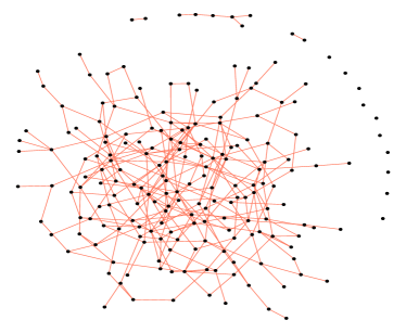
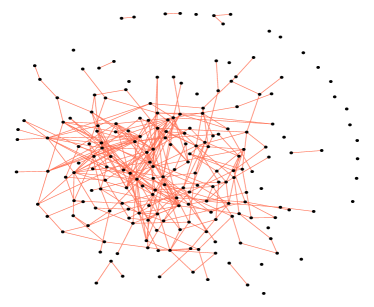
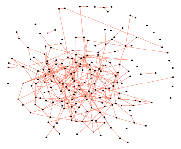
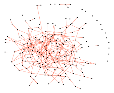
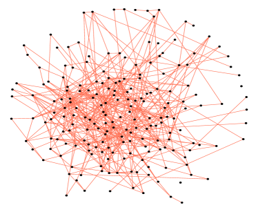
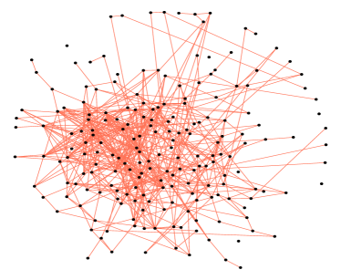
Figure S3: Examples of graph recovery for a random graph of size $d=200$ and $n=300$ samples, where (a) depicts the true graph, (b) is the oracle ($F_{1}=0.79$), (c) is the thAV ($F_{1}=0.89$), (d) is the SCIO (CV) ($F_{1}=0.89$), (e) is the rSME ($F_{1}=0.72$), and (f) is the StARS ($F_{1}=0.65$).

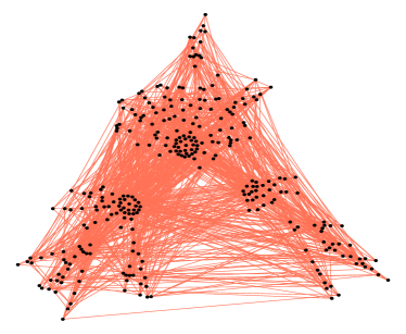
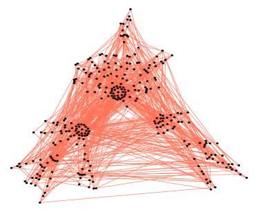
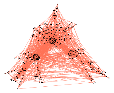
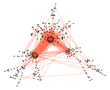
Figure S7: Examples of graph recovery for a scale-free graph of size $d=300$ and $n=200$ samples, where (a) depicts the true graph, (b) is the oracle ($F_{1}=0.25$), (c) is the thAV ($F_{1}=0.23$), (d) is the scaled lasso ($F_{1}=0.27$), (e) is the TIGER ($F_{1}=0.25$), and (f) is the StARS ($F_{1}=0.19$).

We extend the simulations from the main paper to further graphs and number of samples, and compare the $F_{1}$-score, precision, and recall of the oracle, thAV, StARS, scaled lasso, TIGER, rSME using eBIC, SCIO using CV, and SCIO using a Bregman criterion. The results of the experiments in Table 1 are in accordance with the results from the main paper: the thAV estimator is superior to the other methods in $F_{1}$-score (in every but one setting) and achieves often a high precision. Again, the results for recovering a scale-free graph are worse than the results for recovering a random graph. Figures S3 – S8 show examples of the graph recovery performance of various methods in different settings. We can clearly observe that thAV returns a much sparser and more interpretable graph than the other methods. In the case $d=300\text{ and }n=200$, no method is able to recover the graph structure of a scale-free graph, see Figure S7.

Table 2: Similarity $F_{1}(\hat{\Theta}_{C^{\prime}}^{t},\hat{\Theta}_{C^{\prime\prime}}^{t})$ between thAV solutions using different $C$ ($C^{\prime}$ and $C^{\prime\prime}$) for a random graph.

$C$		$0.6$	$0.7$	$0.8$
0.5		0.84 (0.05)	0.68 (0.12)	0.51 (0.21)
0.6		1	0.85 (0.09)	0.67 (0.18)
0.7		-	1	0.79 (0.16)
0.8		-	-	1

(a) $n=200,\,d=300$. The performance scores $F_{1}(\Theta,\hat{\Theta}^{t}_{C})$ are $0.75\,(0.06),\,0.83\,(0.05),\,0.80\,(0.08),\,0.75\,(0.15)$ for $C\in\{0.5,\,0.6,\,0.7,\,0.8\}$, respectively.

$C$		$0.6$	$0.7$	$0.8$
0.5		0.87 (0.06)	0.81 (0.07)	0.80 (0.09)
0.6		1	0.95 (0.03)	0.91 (0.05)
0.7		-	1	0.94 (0.06)
0.8		-	-	1

(b) $n=400,\,d=200$. The performance scores $F_{1}(\Theta,\hat{\Theta}^{t}_{C})$ are $0.81\,(0.04),\,0.91\,(0.04),\,0.94\,(0.02),\,0.94\,(0.03)$ for $C\in\{0.5,\,0.6,\,0.7,\,0.8\}$, respectively.

Dependence on $C$

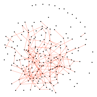
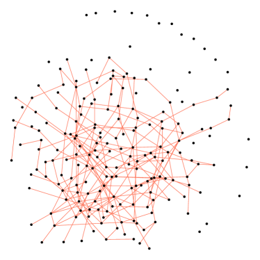
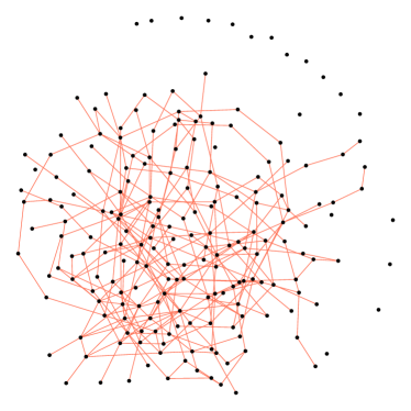
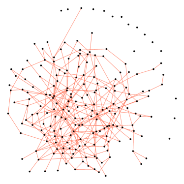
Figure S9: Recovered graphs by the thAV estimator using different values of $C$ for a random graph of size $d=200$ and $n=300$ samples. The graphs in (a) to (d) depict the resulting graphs using $C\in\{0.5,\;0.6,\;0.7,\,0.8\}$, respectively. The corresponding $F_{1}$-scores are $0.78,\;0.88,\;0.94,\;0.95$, respectively.

In this section we show further results demonstrating that the performance of the thAV estimator does not depend decisively on the specific value of $C$. Supplementing the results from Table 3 in the main paper, we investigate the difference in $F_{1}$-score between thAV estimators using different choices for $C$ (see Table 2). We obtain a decent similarity among all estimates and, importantly, the overall $F_{1}(\Theta,\hat{\Theta})$ is always very high so that thAV outperforms competing methods for any choice of $C$. Figures S9 – S14 show some examples of recovered graphs employing the thAV with different $C$. We observe that they look all very similar and we obtain a good $F_{1}$-score, independently of the selected $C$.

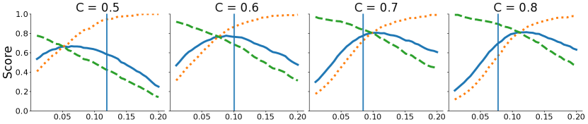
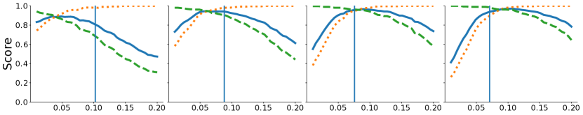
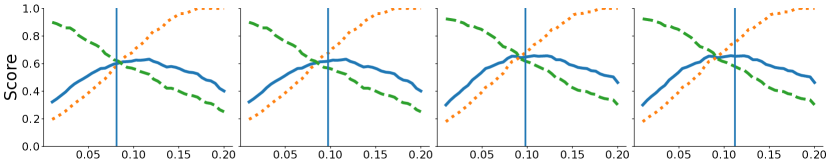
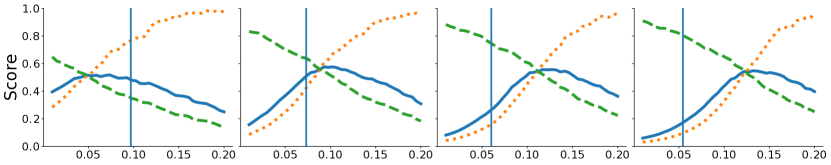
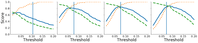
Figure S15: The $F_{1}$-score (blue, solid), precision (yellow, dotted), and recall (green, dashed) of a thresholded AV estimator in various settings. From top to bottom, we consider the settings $n=200,\,d=300$, and $n=400,\,d=200$ for a random graph, $n=300,\,d=200$, and $n=200,\,d=300$, and $n=400,\,d=200$ for a scale-free graph in dependence of the thresholds. The vertical line depicts the proposed threshold $t=C\hat{r}$ corresponding to the thAV estimator.

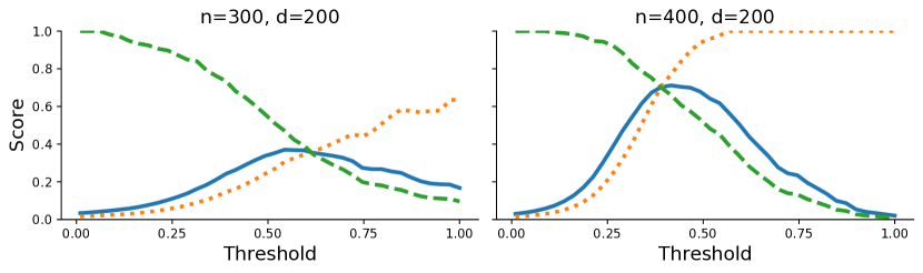
(a) Random graph

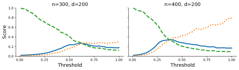
(b) Scale-free graph

Figure S16: The $F_{1}$-score (blue, solid), precision (yellow, dotted), and recall (green, dashed) of a thresholded unregularized estimator in various settings. Note that the unregularized estimator does not exist in the case $d>n$, hence we exclude the setting $d=300,\,n=200$ from this experiment.

Figure S15 supplements the investigations in Figure 1 from the main text. Again, we can observe that the (unthresholded) AV estimator is heavily dependent on the chosen $C$. However after thresholding, all estimators, except of the scale-free graph with $d=300$ using $n=200$ samples, reach a very similar performance plateau. An evident question would be, if it is then even necessary to apply regularization via $r$ instead of employing solely thresholding on the unregularized solution. But note that the unregularized graphical lasso, which is the maximum likelihood estimator, only exists in the setting $d<n$. This is a large restriction in the high-dimensional case. Secondly, we cannot obtain similarly good results for the unregularized thresholded estimator for any threshold, as can be seen in Figure S16. Hence, we claim that it is necessary to combine both regularizations, regularization via regularized optimization and also regularization via thresholding, to obtain good graph recovery results.

C.4 Calibrating other methods via thAV

Table 3: Graph recovery performance for varying graphs and sample size. The bold numbers indicate the best score in each setting.

		random				scale-free
		$F_{1}$	Precision	Recall		$F_{1}$	Precision	Recall
$n=300,\,d=200$
rSME		$\boldsymbol{0.90}$ (0.03)	$\boldsymbol{0.93}$ (0.04)	$\boldsymbol{0.87}$ (0.07)		$\boldsymbol{0.54}$ (0.13)	0.49 (0.19)	$\boldsymbol{0.66}$ (0.14)
sf-glasso		0.70 (0.24)	0.84 (0.18)	0.73 (0.31)		0.52 (0.18)	$\boldsymbol{0.82}$ (0.17)	0.45 (0.22)
$n=200,\,d=300$
rSME		$\boldsymbol{0.81}$ (0.06)	$\boldsymbol{0.82}$ (0.14)	$\boldsymbol{0.83}$ (0.10)		0.27 (0.09)	0.19 (0.07)	$\boldsymbol{0.51}$ (0.15)
sf-glasso		0.61 (0.19)	0.73 (0.16)	0.63 (0.25)		$\boldsymbol{0.31}$ (0.12)	$\boldsymbol{0.77}$ (0.24)	0.24 (0.17)
$n=400,\,d=200$
rSME		$\boldsymbol{0.90}$ (0.08)	$\boldsymbol{0.96}$ (0.04)	$\boldsymbol{0.86}$ (0.12)		$\boldsymbol{0.65}$ (0.14)	0.63 (0.17)	$\boldsymbol{0.70}$ (0.15)
sf-glasso		0.69 (0.27)	0.79 (0.27)	0.79 (0.33)		0.62 (0.17)	$\boldsymbol{0.92}$ (0.07)	0.49 (0.18)

In Section A.1 we have derived a very general foundation for the calibration of regularized optimization problems. In the following empirical study, we tune $2$ other optimization problems for graphical modeling employing the proposed methodology. First, we use the thAV technique to calibrate the regularized score matching estimator (rSME) Lin et al. (2016), which can be employed to recover the conditional dependency structure of a pairwise interaction model. That is, we assume $\boldsymbol{z}$ to have a log-probability density according to

$$\log p(\boldsymbol{z})=\sum_{1\leq i\leq j\leq n}\Theta_{ij}t_{ij}(z_{i},z_{j})-\Psi(\Theta)+b(\boldsymbol{z})$$ (S15)

for sufficient statistics $t_{ij}$, $\Psi$ is a function depending on $\Theta$, and $b$ is the base measure. The model class defined by (S15) includes the Gaussian model, but is much broader. Applying the Hammersley-Clifford theorem, we can derive that similarly to the Gaussian setting it is

$$z_{i}\perp z_{j}|\boldsymbol{z}_{\backslash\{i,j\}}\quad\Leftrightarrow\quad\Theta_{ij}=0.$$

The rSME is motivated by the score matching loss Hyvärinen (2005) and can be reformulated as a the solution of the following optimization problem:

$$\hat{\Theta}_{r}=\operatorname*{\arg\!\min}_{\Theta\in\operatorname{Sym}}\frac{1}{2}\operatorname{vec}\bigl{(}\Theta\bigr{)}^{\top}\Gamma(\boldsymbol{z})\operatorname{vec}\bigl{(}\Theta\bigr{)}+g(\boldsymbol{z})^{\top}\operatorname{vec}\bigl{(}\Theta\bigr{)}+c(\boldsymbol{z})+r\|\Theta\|_{1},$$ (S16)

where $\operatorname{Sym}$ is the set of symmetric matrices in $\mathbb{R}^{D\times D}$, $\operatorname{vec}(\Theta)\in\mathbb{R}^{D^{2}}$ defines the columnwise stacked version of $\Theta$, $\Gamma$ is a symmetric $D^{2}\times D^{2}$ block-diagonal matrix with blocks of size $D\times D$, and $g,c$ are functions mapping $\boldsymbol{z}$ to $\mathbb{R}^{D^{2}}$. For details, we refer to Lemma 2 by Lin et al. (2016). Clearly, (S16) is of the same form as (S1) and Theorem 1 in Lin et al. (2016) justifies Assumption 6. Hence, we can derive similar results for the rSME tuned via the AV technique and threshold similarly to the thAV graphical lasso.

The second type of estimators that we tune via AV is the graphical lasso equipped with a power law regularization Liu and Ihler (2011)

$$\hat{\Theta}_{r}\operatorname*{\arg\!\min}_{\Omega\in\mathcal{S}_{d}^{+}}\biggl{\{}\operatorname*{\operatorname{tr}}\Bigl{[}\frac{1}{n}\sum_{i=1}\bigl{(}\boldsymbol{z}^{(i)}\bigr{)}^{\top}\boldsymbol{z}^{(i)}\Omega\Bigl{]}-\log[\det[\Omega]]+r\sum_{j=1}^{D}\log(\|\Omega_{i\cdot}\|_{1})\biggr{\}},$$ (S17)

where $\Omega_{i\cdot}$ is the $i$th row of $\Omega$. This estimator is designed to learn scale-free graphs in a Gaussian graphical model. In comparison to the rSME, there is no theory about (S17) that justifies Assumption 6. Nonetheless, we applied our calibration scheme for the graphical lasso with power law regularization (sf-glasso).

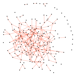
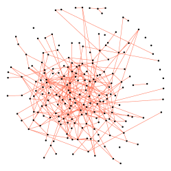
(a) $n=300,\,d=200.$ The resulting $F_{1}$-scores are $0.86$ for the thAV rSME and $0.84$ for the thAV sf-glasso.

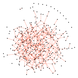
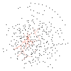
(b) $n=200,\,d=300.$ The resulting $F_{1}$-scores are $0.82$ for the thAV rSME and $0.12$ for the thAV sf-glasso.

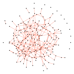
(c) $n=400,\,d=200.$ The resulting $F_{1}$-scores are $0.93$ for the thAV rSME and $0.62$ for the thAV sf-glasso.

Figure S17: Examples of graph recovery for a random graph of varying size and number of samples. Each row depicts (from left to right) the true graph, the thAV rSME, and the thAV sf-glasso, respectively.

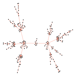
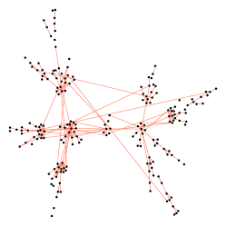
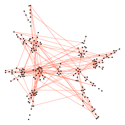
(a) $n=300,\,d=200.$ The resulting $F_{1}$-scores are $0.77$ for the thAV rSME and $0.72$ for the thAV sf-glasso.

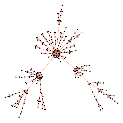
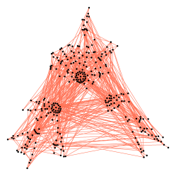
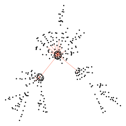
(b) $n=200,\,d=300.$ The resulting $F_{1}$-scores are $0.21$ for the thAV rSME and $0.23$ for the thAV sf-glasso.

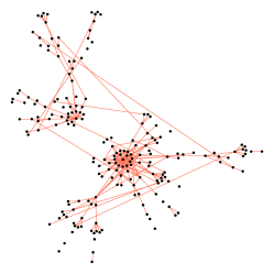
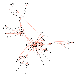
(c) $n=400,\,d=200.$ The resulting $F_{1}$-scores are $0.65$ for the thAV rSME and $0.70$ for the thAV sf-glasso.

Figure S18: Examples of graph recovery for a scale-free graph of varying size and number of samples. Each row depicts (from left to right) the true graph, the thAV rSME, and the thAV sf-glasso, respectively.

The results of the experiments for both estimators are shown in Table 3 (see Section C.2 for computational details). Due to the thresholding, both methods are able to find a good balance between precision and recall. Surprisingly, even though the rSME can be applied to a much broader setting, i.e. in a pairwise interaction model (S15), it performs comparably to the thAV graphical lasso if tuned via the thAV technique. Hence, thAV rSME might be a promising candidate for an application of the general thAV scheme to the non-Gaussian setting. The thAV sf-glasso performs weaker and is less stable. But remarkably, sf-glasso achieves a good precision in recovering a scale-free graph, while maintaining a decent recall. Figure S17 and Figure S18 show some recovered graphs of thAV rSME and thAV sf-glasso.

D Supplement of the Applications

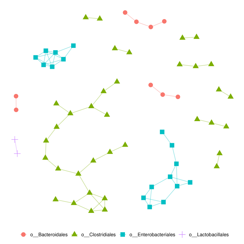
Figure S19: Recovered microbial network based on the American gut data using thAV with the threshold $t:=C\hat{r}$. To avoid too large graphics, we exclude isolated vertices. The color and the shape of a node imply the biological cluster of each OTU.

We present the thAV estimator with threshold $t=C\hat{r}$, applied to the amgut2.filt.phy data from Section 4 in the main paper, in Figure S19. We decided to lower the threshold ($t=0.5C\hat{r}$) in the main paper, because the graph does not include information about interactions across different classes of microbes. But, as already mentioned in the main paper, Corollary $4$ from the main paper is valid for any $\lambda\in(0,3]$.

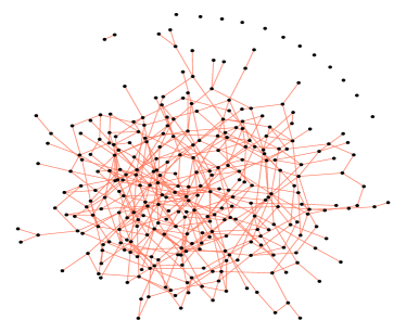
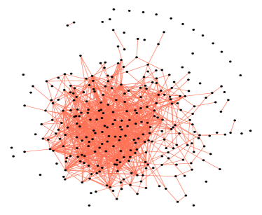
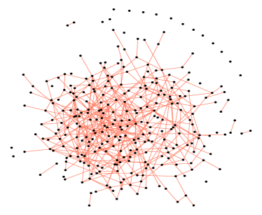
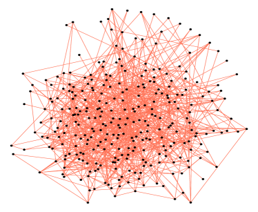
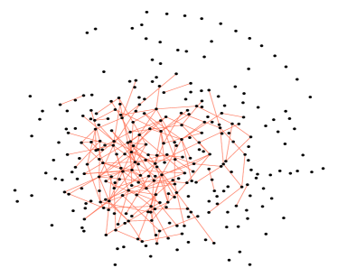
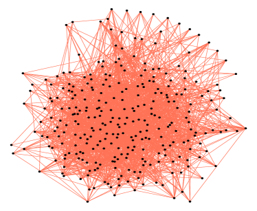
Figure S4: Examples of graph recovery for a random graph of size $d=300$ and $n=200$ samples, where (a) depicts the true graph, (b) is the oracle ($F_{1}=0.49$), (c) is the thAV ($F_{1}=0.86$), (d) is the scaled lasso ($F_{1}=0.66$), (e) is the SCIO (Bregman) ($F_{1}=0.54$), and (f) is the TIGER ($F_{1}=0.39$).

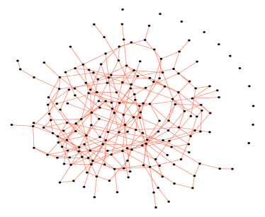
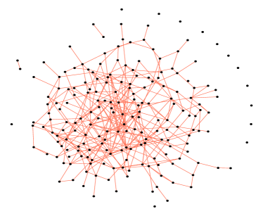
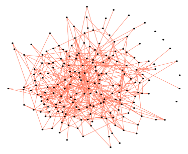
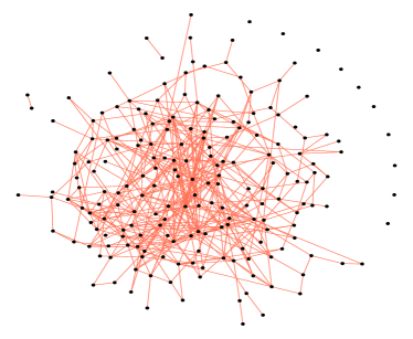
Figure S5: Examples of graph recovery for a random graph of size $d=200$ and $n=400$ samples, where (a) depicts the true graph, (b) is the oracle ($F_{1}=0.86$), (c) is the thAV ($F_{1}=0.96$), (d) is the SCIO (CV) ($F_{1}=0.92$), (e) is the rSME ($F_{1}=0.78$), and (f) is the StARS ($F_{1}=0.76$).

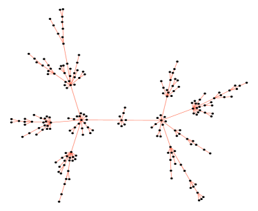
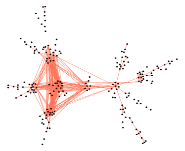
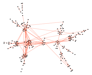
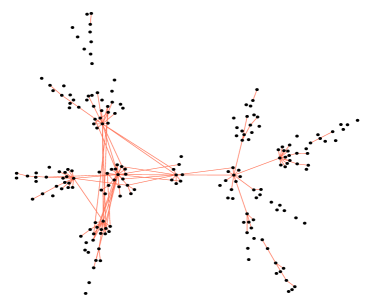
Figure S6: Examples of graph recovery for a scale-free graph of size $d=200$ and $n=300$ samples, where (a) depicts the true graph, (b) is the oracle ($F_{1}=0.42$), (c) is the thAV ($F_{1}=0.73$), (d) is the SCIO (Bregman) ($F_{1}=0.68$), (e) is the rSME ($F_{1}=0.59$), and (f) is the TIGER ($F_{1}=0.50$).

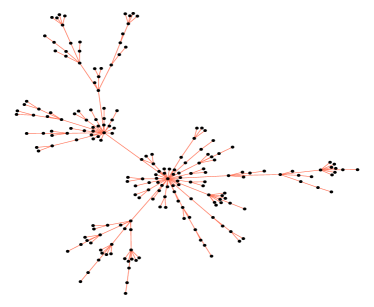
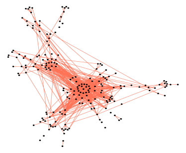
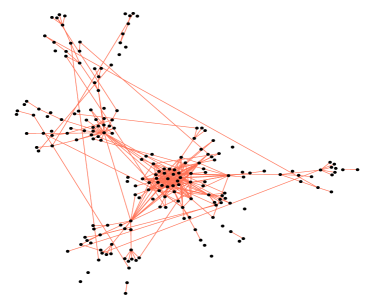
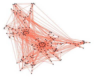
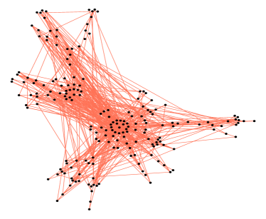
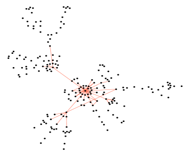
Figure S8: Examples of graph recovery for a scale-free graph of size $d=200$ and $n=400$ samples, where (a) depicts the true graph, (b) is the oracle ($F_{1}=0.34$), (c) is the thAV ($F_{1}=0.60$), (d) is the scaled lasso ($F_{1}=0.43$), (e) is the rSME ($F_{1}=0.42$), and (f) is the SCIO (Bregman) ($F_{1}=0.38$).

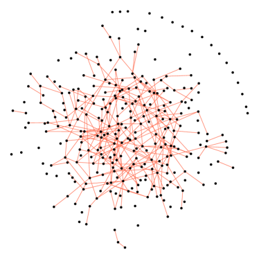
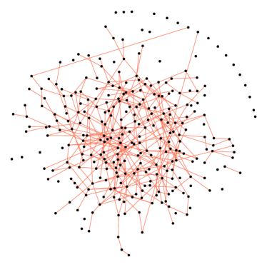
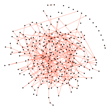
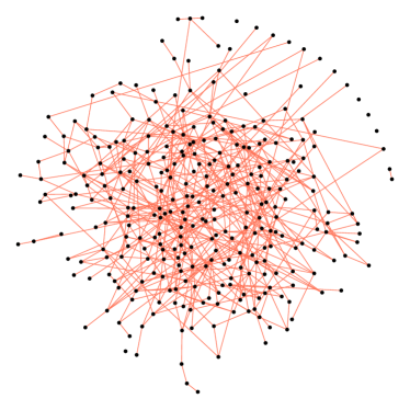
Figure S10: Recovered graphs by the thAV estimator using different values of $C$ for a random graph of size $d=300$ and $n=200$ samples. The graphs in (a) to (d) depict the resulting graphs using $C\in\{0.5,\;0.6,\;0.7,\,0.8\}$, respectively. The corresponding $F_{1}$-scores are $0.74,\;0.82,\;0.86,\;0.84$, respectively.

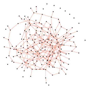
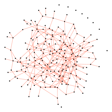
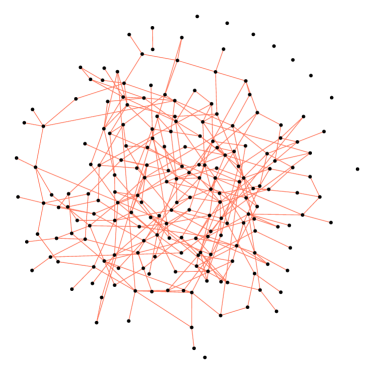
Figure S11: Recovered graphs by the thAV estimator using different values of $C$ for a random graph of size $d=200$ and $n=400$ samples. The graphs in (a) to (d) depict the resulting graphs using $C\in\{0.5,\;0.6,\;0.7,\,0.8\}$, respectively. The corresponding $F_{1}$-scores are $0.82,\;0.94,\;0.97,\;0.96$, respectively.

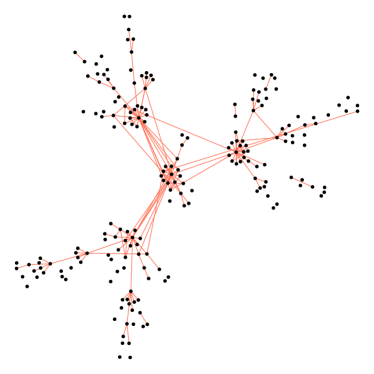
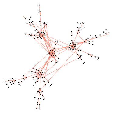
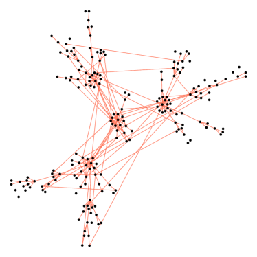
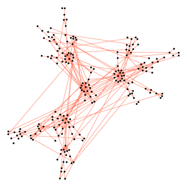
Figure S12: Recovered graphs by the thAV estimator using different values of $C$ for a scale-free graph of size $d=200$ and $n=300$ samples. The graphs in (a) to (d) depict the resulting graphs using $C\in\{0.5,\;0.6,\;0.7,\,0.8\}$, respectively. The corresponding $F_{1}$-scores are $0.69,\;0.73,\;0.75,\;0.71$, respectively.

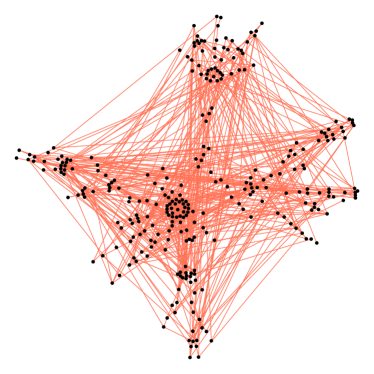
Figure S13: Recovered graphs by the thAV estimator using different values of $C$ for a scale-free graph of size $d=300$ and $n=200$ samples. The graphs in (a) to (d) depict the resulting graphs using $C\in\{0.5,\;0.6,\;0.7,\,0.8\}$, respectively. The corresponding $F_{1}$-scores are $0.30,\;0.17,\;0.11,\;0.13$, respectively.

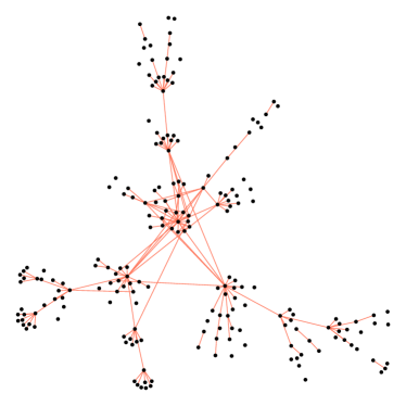
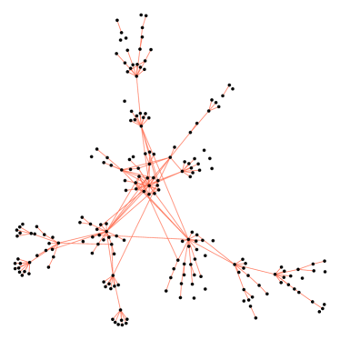
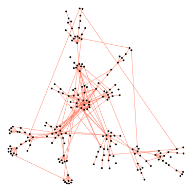
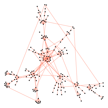
Figure S14: Recovered graphs by the thAV estimator using different values of $C$ for a random graph of size $d=200$ and $n=400$ samples. The graphs in (a) to (d) depict the resulting graphs using $C\in\{0.5,\;0.6,\;0.7,\,0.8\}$, respectively. The corresponding $F_{1}$-scores are $0.75,\;0.83,\;0.80,\;0.85$, respectively.

References

- Banerjee et al. (2007) Onureena Banerjee, Laurent El Ghaoui, and Alexandre d’Aspremont. Model selection through sparse maximum likelihood estimation. 2007. arXiv:0707.0704.
- Barabasi (2016) Albert-Laszlo Barabasi. Network science. Cambridge University Press, 2016.
- Besag (1974) Julian Besag. Spatial interaction and the statistical analysis of lattice systems. J. R. Stat. Soc. Ser. B. Stat. Methodol., 36(2):192–225, 1974.
- Boyd and Vandenberghe (2009) Stephen P. Boyd and Lieven Vandenberghe. Convex optimization. Cambridge Univ. Press, 2009.
- Bu and Lederer (2017) Yunqi Bu and Johannes Lederer. Integrating additional knowledge into estimation of graphical models. 2017. arXiv:1704.02739.
- Bühlmann et al. (2014) Peter Bühlmann, Markus Kalisch, and Lukas Meier. High-dimensional statistics with a view toward applications in biology. Annu. Rev. Stat. Appl., 1(1):255–278, 2014.
- Caballe et al. (2015) Adria Caballe, Natalia Bochkina, and Claus Mayer. Selection of the regularization parameter in graphical models using network characteristics. 2015. arXiv:1509.05326.
- Chichignoud et al. (2014) Michaël Chichignoud, Johannes Lederer, and Martin Wainwright. A practical scheme and fast algorithm to tune the lasso with optimality guarantees. 2014. arXiv:1410.0247.
- Denev (2015) Alexander Denev. Probabilistic graphical models: A new way of thinking in financial modelling. Risk Books, 2015.
- Dezeure et al. (2015) Ruben Dezeure, Peter Buehlmann, Lukas Meier, and Nicolai Meinshausen. High-dimensional inference: Confidence intervals, p-values and R-software hdi. Statist. Sci., pages 533–558, 2015.
- Dobra et al. (2004) Adrian Dobra, Chris Hans, Beatrix Jones, Joseph R. Nevins, Guang Yao, and Mike West. Sparse graphical models for exploring gene expression data. J. Multivariate Anal., 90(1):196–212, 2004.
- Fan et al. (2009) Jianqing Fan, Yang Feng, and Yichao Wu. Network exploration via the adaptive lasso and scad penalties. Ann. Appl. Stat., 3(2):521–541, 2009.
- Fan et al. (2016) Jianqing Fan, Yuan Liao, and Han Liu. An overview of the estimation of large covariance and precision matrices. Econom. J., 19(1):C1–C32, 2016.
- Friedman et al. (2008) Jerome Friedman, Trevor Hastie, and Robert Tibshirani. Sparse inverse covariance estimation with the graphical lasso. Biostatistics, 9(3):432–441, 2008.
- Gilbert (1959) E. N. Gilbert. Random graphs. Ann. Math. Stat., 30(4):1141–1144, 1959.
- Grimmett (1973) G. R. Grimmett. A theorem about random fields. Bull. Lond. Math. Soc., 5:81–84, 1973.
- Hoerl and Kennard (2000) Arthur E. Hoerl and Robert W. Kennard. Ridge regression: Biased estimation for nonorthogonal problems. Technometrics, 42(1):80–86, 2000.
- Hyvärinen (2005) Aapo Hyvärinen. Estimation of non-normalized statistical models by score matching. J. Mach. Learn. Res., 6(1):695–709, 2005.
- Jeong et al. (2001) H. Jeong, S. P. Mason, A. L. Barabási, and Z. N. Oltvai. Lethality and centrality in protein networks. Nature, 411(6833):41–42, 2001.
- Kurtz et al. (2015) Zachary D. Kurtz, Christian L. Müller, Emily R. Miraldi, Dan R. Littman, Martin J. Blaser, and Richard A. Bonneau. Sparse and compositionally robust inference of microbial ecological networks. PLoS Comput. Biol., 11(5):e1004226, 2015.
- Lauritzen (1996) Steffen L. Lauritzen. Graphical models, volume 17 of Oxford statistical science series. Clarendon, 1996.
- Lin et al. (2016) Lina Lin, Mathias Drton, and Ali Shojaie. Estimation of high-dimensional graphical models using regularized score matching. Electron. J. Stat., 10(1):806, 2016.
- Liu and Wang (2017) Han Liu and Lie Wang. Tiger: A tuning-insensitive approach for optimally estimating gaussian graphical models. Electron. J. Stat., 11(1):241–294, 2017.
- Liu et al. (2009) Han Liu, John Lafferty, and Larry Wasserman. The nonparanormal: Semiparametric estimation of high dimensional undirected graphs. J. Mach. Learn. Res., 10:2295–2328, 2009.
- Liu et al. (2010) Han Liu, Kathryn Roeder, and Larry Wasserman. Stability approach to regularization selection (stars) for high dimensional graphical models. Adv. Neural Inf. Process. Syst., 24 2:1432–1440, 2010.
- Liu and Ihler (2011) Qiang Liu and Alexander Ihler. Learning scale free networks by reweighted l1 regularization. Proc. Mach. Learn. Res., 15:40–48, 2011.
- Liu and Luo (2015) Weidong Liu and Xi Luo. Fast and adaptive sparse precision matrix estimation in high dimensions. J. Multivariate Anal., 135:153 – 162, 2015.
- McDonald et al. (2018) Daniel McDonald, Embriette Hyde, Justine W. Debelius, James T. Morton, Antonio Gonzalez, and et al. Ackermann. American gut: An open platform for citizen science microbiome research. mSystems, 3(3):e00031–18, 2018.
- Meinshausen and Bühlmann (2006) Nicolai Meinshausen and Peter Bühlmann. High-dimensional graphs and variable selection with the lasso. Ann. Statist., 34(3):1436–1462, 2006.
- Ravikumar et al. (2011) Pradeep Ravikumar, Martin J. Wainwright, Garvesh Raskutti, and Bin Yu. High-dimensional covariance estimation by minimizing l1-penalized log-determinant divergence. Electron. J. Stat., 5:935–980, 2011.
- Sun (2019) Tingni Sun. scalreg: Scaled Sparse Linear Regression, 2019. R package version 1.0.1.
- Sun and Zhang (2012) Tingni Sun and Cun-Hui Zhang. Sparse matrix inversion with scaled lasso. J. Mach. Learn. Res., 14, 02 2012.
- Tang et al. (2015) Qingming Tang, Siqi Sun, and Jinbo Xu. Learning scale-free networks by dynamic node specific degree prior. ICML, 37:2247–2255, 2015.
- Thieffry et al. (1998) Denis Thieffry, Araceli M. Huerta, Ernesto Pérez-Rueda, and Julio Collado-Vides. From specific gene regulation to genomic networks: A global analysis of transcriptional regulation in escherichia coli. BioEssays, 20(5):433–440, 1998.
- Tibshirani (1996) Robert Tibshirani. Regression shrinkage and selection via the lasso. J. R. Stat. Soc. Ser. B. Stat. Methodol., 58(1):267–288, 1996.
- Wainwright (2019) Martin J. Wainwright. High-dimensional statistics: A non-asymptotic viewpoint, volume 48. Cambridge University Press, 2019.
- Witten et al. (2011) Daniela M. Witten, Jerome H. Friedman, and Noah Simon. New insights and faster computations for the graphical lasso. J. Comput. Graph. Statist., 20(4):892–900, 2011.
- Yoon et al. (2019) Grace Yoon, Irina Gaynanova, and Christian L. Müller. Microbial networks in spring - semi-parametric rank-based correlation and partial correlation estimation for quantitative microbiome data. Front. Genet., 10:516, 2019.
- Yu et al. (2019) Shiqing Yu, Mathias Drton, and Ali Shojaie. Generalized score matching for non-negative data. J. Mach. Learn. Res., 2019.
- Yuan and Lin (2007) M. Yuan and Y. Lin. Model selection and estimation in the gaussian graphical model. Biometrika, 94(1):19–35, 2007.
- Zhang (2010) Cun-Hui Zhang. Nearly unbiased variable selection under minimax concave penalty. Ann. Statist., 38(2):894–942, 2010.
- Zhao et al. (2012) Tuo Zhao, Han Liu, Kathryn Roeder, John Lafferty, and Larry Wasserman. The huge package for high-dimensional undirected graph estimation in r. J. Mach. Learn. Res., 13:1059–1062, 2012.
- Zhuang and Lederer (2018) Rui Zhuang and Johannes Lederer. Maximum regularized likelihood estimators: A general prediction theory and applications. Stat, 7(1):e186, 2018.
Supplementary Files: