Three Exceptions to the Grossman-Nir Bound

Abstract

We show that the Grossman-Nir (GN) bound, $\text{Br}(K_{L}\to\pi^{0}\nu\bar{\nu})\leq 4.3\,\text{Br}(K^{+}\to\pi^{+}\nu\bar{\nu})$, can be violated in the presence of light new physics with flavor violating couplings. We construct three sample models in which the GN bound can be violated by orders of magnitude, while satisfying all other experimental bounds. In the three models the enhanced branching ratio $\text{Br}(K_{L}\to\pi^{0}+{\rm inv})$ is due to $K_{L}\to\pi^{0}\phi_{1}$, $K_{L}\to\pi^{0}\phi_{1}\phi_{1}$, $K_{L}\to\pi^{0}\psi_{1}\bar{\psi}_{1}$ transitions, respectively, where $\phi_{1}(\psi_{1})$ is a light scalar (fermion) that escapes the detector. In the three models $\text{Br}(K^{+}\to\pi^{+}+{\rm inv})$ remains very close to the SM value, while $\text{Br}(K_{L}\to\pi^{0}+{\rm inv})$ can saturate the present KOTO bound. Besides invisible particles in the final state (which may account for dark matter) the models require additional light mediators around the GeV-scale.

1 Introduction

In the SM, the $K_{L}\to\pi^{0}\nu\bar{\nu}$ and $K^{+}\to\pi^{+}\nu\bar{\nu}$ decays proceed through the same short distance operator, involving the fields of the quark level transition ($s\to d\nu\bar{\nu}$). The matrix elements for the $K_{L}\to\pi^{0}\nu\bar{\nu}$ and $K^{+}\to\pi^{+}\nu\bar{\nu}$ transitions are thus trivially related through isospin, leading to the Grossman-Nir (GN) bound Grossman and Nir (1997)

$$\text{Br}(K_{L}\to\pi^{0}\nu\bar{\nu})\leq 4.3\,\text{Br}(K^{+}\to\pi^{+}\nu\bar{\nu}).$$ (1)

The bound remains valid in the presence of heavy New Physics (NP), i.e., for NP modification due to new particles with masses well above the kaon mass. The bound is saturated for the case of maximal CP violation, if lepton flavor violation can be neglected (see Ref. Grossman et al. (2004) for counter-examples).

In this paper we investigate to what extent NP contributions to $K\to\pi+{\rm inv}$ decays can violate the GN bound. Simple dimensional counting shows that for large violations of the GN bound the NP needs to be light, of order of a few GeV at most (see Section 2 and Refs. He et al. (2020); Li et al. (2020)). Such light NP faces stringent experimental constraints from rare meson decays and collider/beam dump searches as well as from astrophysics and cosmology. Nevertheless, the couplings needed to modify the rare $K\to\pi+{\rm inv}$ decays are small enough that interesting modifications of the GN bound are indeed possible. We identify three sample models that achieve this through the following decays:

• Model 1: $K_{L}\to\pi^{0}\phi_{1}$, where the mass of the light scalar, $\phi_{1}$, can be anywhere from $m_{\phi_{1}}\lesssim m_{K}-m_{\pi}$ to a few MeV or even less,

• Model 2: $K_{L}\to\pi^{0}\phi_{1}\phi_{1}$, where the mass of the light scalar, $\phi_{1}$, is required in a large part of the parameter space to be $m_{\phi_{1}}\gtrsim m_{\pi}/2$ in order to avoid constraints from invisible pion decays,

• Model 3: $K_{L}\to\pi^{0}\psi_{1}\bar{\psi}_{1}$, with $\psi_{1}$ a light fermion whose mass is required to be $m_{\psi_{1}}\gtrsim m_{\pi}/2$ in most of the phenomenologically viable parameter space.

The $\phi_{1}$ and $\psi_{1}$ particles are feebly interacting and escape the detector, resulting in the $K_{L}\to\pi^{0}+{\rm inv}$ signature, as does the SM transition, $K_{L}\to\pi^{0}\nu\bar{\nu}$. The NP is thus detected through an enhanced $\Gamma(K_{L}\to\pi^{0}+{\rm inv})$ rate. Furthermore, the three models can be distinguished from the SM and each other by measuring the energy distribution of the neutral pion, $d\Gamma(K_{L}\to\pi^{0}+{\rm inv})/dE_{\pi}$, see Fig. 1 for several sample distributions. While the two body decay in Model 1 results in a fixed pion energy, the three body decays in Model 2 and 3 can be close to the SM distribution for light $\phi_{1}$ and $\psi_{1}$ masses and differ from it for non-negligible masses. Let us mention in passing that the lightness of the scalars could be due to them being a pseudo Goldstone boson of a broken global symmetry whereas for fermions light masses are natural due to chiral symmetry.

In all three models the branching ratio $\text{Br}(K^{+}\to\pi^{+}+{\rm inv})$ remains close to the SM value, $\text{Br}(K^{+}\to\pi^{+}\nu\bar{\nu})_{\rm SM}=(8.4\pm 1.0)\times 10^{-11}$ Buras et al. (2005); Brod et al. (2011); Buras et al. (2015), and thus below the preliminary NA62 bound $\text{Br}(K^{+}\to\pi^{+}\nu\bar{\nu})_{\rm exp}<1.85\times 10^{-10}$ Volpe , while $\text{Br}(K_{L}\to\pi^{0}+{\rm inv})$ can be enhanced well above its SM value, $\text{Br}(K_{L}\to\pi^{0}\nu\bar{\nu})_{\rm SM}=(3.4\pm 0.6)\times 10^{-11}$  Buras et al. (2005); Brod et al. (2011); Buras et al. (2015). The NP induced $K_{L}\to\pi^{0}+{\rm inv}$ transitions, on the other hand, can saturate the present experimental upper bounds. The exact experimental bounds depend on the assumed NP decay channel. For instance, for the SM decay kinematics KOTO obtains $\text{Br}(K_{L}\to\pi^{0}\nu\bar{\nu})_{\rm exp}<3.0\times 10^{-9}$ Ahn et al. (2019), while for two body decays the bound is somewhat stronger, $\text{Br}(K_{L}\to\pi^{0}\nu\bar{\nu})_{\rm exp}<2.4\times 10^{-9}$, for $m_{\phi_{1}}\lesssim m_{\pi}$ Ahn et al. (2019). Recently, KOTO unblinded its 2016-18 data and found four events in the signal region, while only $0.05\pm 0.02$ background events were expected Shinohara (under additional scrutiny this has been revised to $0.34\pm 0.08$ expected background events Nomura ). If the preliminary data are interpreted as a signal, they correspond to a rate $\text{Br}(K_{L}\to\pi^{0}+{\rm inv})_{\rm KOTO}=\big{(}2.1^{+2.0}_{-1.1}\big{)}\times 10^{-9}$ Kitahara et al. (2020). Note, that while some of the observed events may be due to yet unidentified backgrounds – according to KOTO the four events do have some suspicious features – they cannot be conclusively rejected Nomura . As a useful benchmark we will thus compare our results also with $\text{Br}(K_{L}\to\pi^{0}+{\rm inv})_{\rm KOTO}$ as though these events are due to NP. Furthermore, in the numerics we quote the experimental bounds on three body decays, $K\to\pi\phi_{1}\phi_{1}$ $K\to\pi\psi_{1}\bar{\psi}_{1}$, assuming the experimental efficiencies are the same as for the SM $K\to\pi\nu\bar{\nu}$ transition. In reality, we expect the bounds to be weaker, since the experimental efficiencies are highest for larger values of $E_{\pi}$, while NP decays considered here are less peaked towards maximal $E_{\pi}$ (as compared to the SM).

The three models considered in this work differ from the other proposed NP solutions to the KOTO anomaly in that they allow for large violations of the GN bound at the level of the amplitudes already. In contrast, Ref. Fabbrichesi and Gabrielli (2019) relies on the fact that the available phase space is larger for neutral kaon decays due to $m_{K_{L}}-m_{\pi^{0}}>m_{K^{+}}-m_{\pi^{+}}$ and thus $K^{+}\to\pi^{+}X_{\rm inv}$ decays can be forbidden by a finely tuned choice for the mass of the invisible final state $X_{\rm inv}$. Ref. Kitahara et al. (2020) instead obtains, in one of the models, an apparent violation of the GN bound from the experimental set-up; the produced light NP particles decay on experimental length-scales, and are not observed in NA62 but are observed in KOTO due to the geometry of the experiments. Finally, the NP models of Refs. Kitahara et al. (2020); Fuyuto et al. (2015); Hou (2017); Egana-Ugrinovic et al. (2019); Dev et al. (2020); Jho et al. (2020); Liu et al. (2020); Cline et al. (2020); Liao et al. (2020) do not violate the GN bound, but can allow for a large signal in KOTO since NA62 is not sensitive to $X_{\rm inv}$ with a mass close to the pion mass.

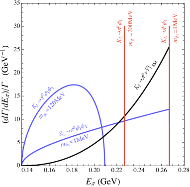
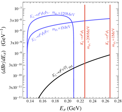
Figure 1: Left: The normalized decay width distributions as functions of the pion energy, $E_{\pi}$, for the SM (black line), for the decay dominated by the two body NP transition (Model 1), $K_{L}\to\pi^{0}\phi_{1}$, for two choices of invisible scalar masses, $m_{\phi_{1}}=1$ MeV, 200 MeV (red lines) and for three body NP decay (Model 2), $K_{L}\to\pi^{0}\phi_{1}\phi_{1}$, with $m_{\phi_{1}}=1$ MeV, 120 MeV (blue lines). Right: The branching ratio distributions, where NP contributions saturate the present KOTO bound Ahn et al. (2019). At the kinematic endpoint, $E_{\pi}\to m_{\pi}$, we have $d\Gamma_{\textrm{SM}}\propto p_{\pi}^{3}dE_{\pi}$ while for NP Model 2 $d\Gamma_{K_{L}\to\pi^{0}\phi_{1}\phi_{1}}\propto p_{\pi}dE_{\pi}$, where $p_{\pi}=(E_{\pi}^{2}-m_{\pi}^{2})^{1/2}$ (similarly for Model 3, Section 5, $d\Gamma_{K_{L}\to\pi^{0}\psi_{1}\bar{\psi}_{1}}\sim p_{\pi}dE_{\pi}$ unless the Yukawa couplings $y_{ij}$ are purely real). This follows from the partial wave expansion, $d\Gamma/dE_{\pi}\sim p_{\pi}^{2l+1}$, adapted to EFTs Hiller and Zwicky (2014). In the $K\to\pi\nu\bar{\nu}$ rate the $V$-$A$ SM interaction induces a negligible $S$-wave contribution proportional to the neutrino mass, whereas the scalar interactions in our model induce a non-suppressed $S$-wave. The maximum recoil, $E_{\pi}\to E_{\pi}\big{|}_{\rm max}$, in contrast, is controlled by a single power of the $\nu$/$\phi_{1}$-velocity in the $q^{\mu}$ rest frame, $\beta_{\nu,\phi_{1}}=(1-4m^{2}_{\nu/\phi_{1}}/q^{2})^{1/2}$ (where $q^{2}=m_{K}^{2}+m_{\pi}^{2}-2m_{K}E_{\pi})$. For small $m_{\nu}/\phi_{1}$ this velocity goes to $1$ for most values of $q^{2}$, leading to a sharp cut-off at $E_{\pi}\big{|}_{\rm max}$.

The paper is organized as follows. In section 2 a general Effective Field Theory analysis is presented. The three models are discussed consecutively in Sections 3, 4 and 5 with the main plots collected in Figs. 5, 6, in Figs. 15, 16 and in Figs. 19, 20 for Model 1, 2 and 3, respectively, with constraints due to $K^{0}-\bar{K}^{0}$ mixing, cosmology and invisible pion decays discussed in the respective sections. The paper ends with conclusions in Section 6, while details on decay rates and integral conventions are deferred to two short appendices.

2 The EFT analysis

We first perform an Effective Field Theory (EFT) based analysis, assuming that the SM is supplemented by a single light scalar, $\varphi$, while any other NP states are heavy and integrated out. The light scalar has flavor violating couplings and is created in the $K^{0}\to\pi^{0}\varphi$ decay. The effective Lagrangian inducing this transition is given by

$${\cal L}_{\rm eff}=c^{(4)}\big{(}\bar{s}d\big{)}\varphi+\sum_{i}\frac{c_{i}^{(7)}}{\Lambda^{3}}\big{(}\bar{s}\Gamma_{i}d\big{)}\big{(}\bar{d}\Gamma_{i}^{\prime}d\big{)}\varphi+\cdots\;,$$ (2)

where we only keep the parity-even operators of lowest dimension and work in the quark mass basis. There is a single dimension 4 operator, and the sum runs over the dimension 7 operators, where $\Gamma_{i},\Gamma_{i}^{\prime}$ include both Dirac and color structures. In (2) solely parity even operators, relevant the $K\to\pi$ decay, are displayed. Moreover, ${\cal O}^{(5)}=(\bar{s}\gamma_{\mu}d)\partial_{\mu}\varphi$ can be traded for the dimension 4 operator ${\cal O}^{(4)}=(m_{s}-m_{d})(\bar{s}d)\varphi$, by use of the equations of motion (EOMs). Similarly, the EOM $\bar{s}\overset{\leftrightarrow}{D}_{\mu}d=-\partial^{\nu}(\bar{s}i\sigma_{\mu\nu}d)+i(m_{s}+m_{d})\bar{d}\gamma_{\mu}d$ allows us to replace ${\cal O}^{(6)}=(\bar{s}\overset{\leftrightarrow}{D}_{\mu}d)\partial^{\mu}\varphi$ with the same operator $(m_{s}^{2}-m_{d}^{2})\bar{s}d\varphi$. This leaves the dimension 4 and dimension 7 operators in (2) as operators of lowest dimension.

At the quark level the dimension 4 operator induces the $s\to d\varphi$ transition and thus contributes equally to $K^{0}\to\pi^{0}\varphi$ and $K^{+}\to\pi^{+}\varphi$ decays, see the first diagram in Fig. 2. The resulting matrix elements for the $K_{L}\to\pi^{0}\varphi$ and $K^{+}\to\pi^{+}\varphi$ decays are

$$\{{\cal M}^{(4)}(K_{L}\to\pi^{0}\varphi),{\cal M}^{(4)}(K^{+}\to\pi^{+}\varphi)\}=\frac{m_{K}^{2}-m_{\pi}^{2}}{m_{s}-m_{d}}f_{+}(0)\{\operatorname{Im}c^{(4)},c^{(4)}\}.$$ (3)

The $K_{L}\to\pi^{0}\varphi$ decay is CP violating and vanishes in the limit of zero weak phases, $\operatorname{Im}c^{(4)}\to 0$. These contributions therefore obey the Grossman-Nir relation,

$$|{\cal M}^{(4)}(K_{L}\to\pi^{0}\varphi)|\leq|{\cal M}^{(4)}(K^{+}\to\pi^{+}\varphi)|.$$ (4)

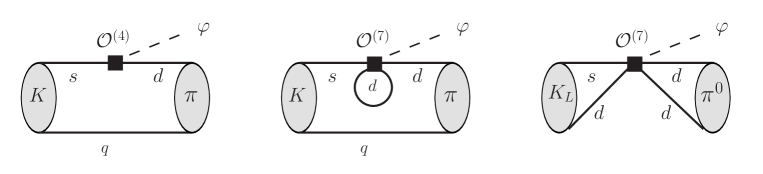
Figure 2: Contributions from dimension 4 (first diagram) and dimension 7 (2nd and 3rd diagrams) EFT operators to the $K\to\pi\varphi$ transition. The last diagram contributes to $K_{L}\to\pi^{0}\varphi$ only. The quark-loop diagram in the middle corresponds to the $S,E$ classes of diagrams and the weak annihilation diagram on the right to the $W,C$ classes of diagrams in the lattice computation of Ref. Christ et al. (2016).

The dimension 7 operators, on the other hand, contribute to $K^{0}\to\pi^{0}\varphi$ and $K^{+}\to\pi^{+}\varphi$ decays in a qualitatively different way. The $K_{L}\to\pi^{0}\varphi$ decay can proceed through the weak annihilation type contractions of valence quarks, i.e., through the third diagram in Fig. 2. The $K^{+}\to\pi^{+}\varphi$ transition requires the $\bar{d}d$ internal line to close in a loop (cf. the 2nd diagram in Fig. 2). Such contractions also contribute to $K_{L}\to\pi^{0}\varphi$. Using at first perturbative counting the latter contributions are suppressed, giving parametric estimates

$$\{{\cal M}^{(7)}(K_{L}\to\pi^{0}\varphi),{\cal M}^{(7)}(K^{+}\to\pi^{+}\varphi)\}\propto\frac{m_{K}^{3}}{\Lambda^{3}}\Big{\{}\operatorname{Im}c_{i}^{(7)},\frac{1}{(4\pi)^{2}}\Big{(}\frac{\alpha_{s}}{4\pi}\big{)}^{n}c_{i}^{(7)}\Big{\}},$$ (5)

where we neglected $m_{\pi}$ compared to $m_{K}$ and do not write factors that are parametrically of the same size but may differ by ${\mathcal{O}}(1)$, such as different form factors in the two cases. Depending on the Dirac-color structures $\Gamma^{(^{\prime})}_{i}$ of the operator one or more gluon exchanges may be required leading to additional $(\alpha_{s}/4\pi)^{n}$-factors shown in (5).

A priori this leaves two classes of NP models with potentially sizeable violations of the GN bound. The first possibility is heavy NP, with a suppressed $c^{(4)}$ Wilson coefficient such that dimension 7 operators dominate. The other possibility is light NP such that the EFT assumption, on which the above analysis is based on, is violated.

Building viable heavy NP models that violate the GN bound faces several obstacles. First of all, $c^{(4)}$ would have to be heavily suppressed, $c^{(4)}\ll m_{q}/\Lambda$, well below naive expectations. If this is not the case, the “heavy” NP scale needs to be quite light. For instance, for $c^{(4)}\sim m_{q}/\Lambda$, $c_{i}^{(7)}\sim{\mathcal{O}}(1)$ the dimension 4 operator contributions dominate over the dimension 7 ones already for $\Lambda\gtrsim{\mathcal{O}}(3{\rm~{}GeV})$ (see also the discussion in He et al. (2020)). Furthermore, even if the hierarchy $c^{(4)}\ll c^{(7)}$ was realised, it is not clear whether the GN bound could be violated by more than a factor of a few. The scaling estimates in (5) were based on perturbative expansion, while the kaon decays are in the deep non-perturbative regime of QCD. One can get an idea of the size of the ${\cal M}_{K}^{(7)}\propto\langle\pi\varphi|{\cal O}^{(7)}|K\rangle$ matrix elements by linking them to the ones for $K\to\pi\ell^{+}\ell^{-}$ decays that were explored in lattice QCD for light quark masses above their physical value ($m_{\pi}=430~{}\text{MeV}$ and $m_{K}=625~{}\text{MeV}$) Christ et al. (2016). Figure 5 in Ref. Christ et al. (2016) indicates that the quark-loop and weak annihilation contractions, corresponding to the middle and the right diagrams in Fig. 2, lead to contributions of comparable size, contrary to the perturbative expectations in (5). If these results carry over to $K\to\pi\varphi$ decays, it would seem that the ratio of ${\cal M}^{(7)}(K_{L}\to\pi^{0}\varphi)/{\cal M}^{(7)}(K^{+}\to\pi^{+}\varphi)$ would not easily exceed a factor of $\sim 2$ in models of heavy NP. It is unclear, however, whether this qualitative feature, based on the evaluation of the SM $V-A$ four quark operators Christ et al. (2016), would carry over to a model with scalar-scalar four quark operators, originating from a scalar mediator. For instance, for $V-A$ operators the weak annihilation topology is chirally suppressed in the factorisation approximation, while this is not the case for scalar operators.

In conclusion, for heavy mediators the GN bound might or might not be violated in the case $c^{(4)}\ll c^{(7)}$. In this manuscript we therefore focus on the second possibility, the possibility of light NP mediators, where we can use Chiral Perturbation Theory (ChPT) with light NP states as a reliable tool to make predictions.

3 Model 1 - scalar model leading to two-body kaon decays

In the first example we introduce two real scalar fields, $\phi_{1}$ and $\phi_{2}$. The enhancement of the $K\to\pi$+inv branching ratio over the SM is due to the $K\to\pi\phi_{1}$ decay, while $K\to\pi\phi_{2}$ is kinematically forbidden, i.e., we take $m_{\phi_{2}}>m_{K}-m_{\pi}$. The $\phi_{1}$ interacts feebly with matter and escapes the detector, resulting in a missing momentum signature. The relevant terms in the Lagrangian are

$${\cal L}\supset g_{qq^{\prime}}^{(i)}(\bar{q}_{L}q_{R}^{\prime})\phi_{i}+{\rm h.c.}+\lambda m_{S}\phi_{2}^{2}\phi_{1}\;,$$ (6)

where $q,q^{\prime}=\{u,d,s\}$ and summation over repeated indices is implied. The couplings $g_{qq^{\prime}}^{(i)}$ are complex, and their imaginary parts trigger the $K_{L}\to\pi^{0}\phi_{1}$ decay.

Large violations of the GN bound arise when there is a large hierarchy among the following couplings,

$$g_{sd}^{(1)}\ll g_{sd}^{(2)}\ll g_{dd}^{(2)},$$ (7)

while all other couplings are further suppressed. In our benchmarks these remaining couplings as well as $g_{sd}^{(1)}$ will be set to zero. Before proceeding to predictions for branching ratios and the numerical analysis, it is instructive to perform a naive dimensional analysis (NDA). This will give us insight into why large violations of the GN bound are possible as well as to how large these violations can possibly be.

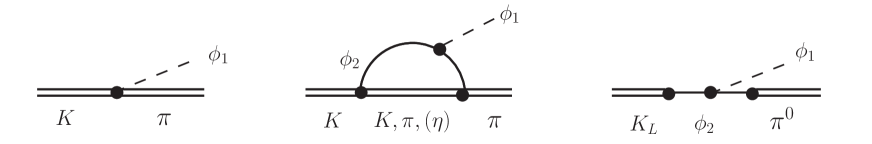
Figure 3: Diagrams for the $K\to\pi\phi_{1}$ decay in Model 1 with the GN-violating contribution to the very right. These diagrams enter the matrix elements in Eqs. (18), (19). Note that the $\eta$ in the loop contributes to the $K_{L}$ decay only. Diagrams which we neglect, such as the diagrams of ${\mathcal{O}}(p^{4})$ or ${\mathcal{O}}(g_{qq^{\prime}}^{3})$, are not shown.

Taking $m_{S}\sim m_{\phi_{2}}\sim m_{K}$ the NDA estimate for the two decay amplitudes are,

$${\cal M}(K_{L}\to\pi^{0}\phi_{1}) \;\propto\; \operatorname{Im}\ g_{sd}^{(1)}+{\mathcal{O}}(1)\times\lambda\operatorname{Re}g_{sd}^{(2)}\operatorname{Im}g_{dd}^{(2)}\;,$$ (8)

$${\cal M}(K^{+}\to\pi^{+}\phi_{1}) \;\propto\; g_{sd}^{(1)}+{\mathcal{O}}(1)\times\frac{1}{16\pi^{2}}\lambda\,g_{sd}^{(2)}g_{dd}^{(2)}\;,$$ (9)

where the first term in each line is due to the 1st diagram in Fig. 3. The second term in (8) is due to the 3rd diagram in Fig. 3, which is absent in the $K^{+}\to\pi^{+}\phi_{1}$ decay. This is the crucial difference between the two decays and leads to large violations of the GN bound, provided $g_{sd}^{(1)}$ is small.

However, violations of the GN bound cannot be arbitrarily large. Even if $g_{sd}^{(1)}$ is set to zero, the $K^{+}\to\pi^{+}\phi_{1}$ transition is generated at the loop level from the 2nd diagram in Fig. 3, giving the 2nd term in (9). Without fine-tuning the ratio ${\cal M}(K_{L}\to\pi^{0}\phi_{1})/{\cal M}(K^{+}\to\pi^{+}\phi_{1})$ is thus at best as large as the loop factor, $16\pi^{2}\sim 10^{3}$. Taking into account the present experimental results, this is more than enough to saturate the present KOTO bound while only marginally modifying the $K^{+}\to\pi^{+}+$inv decay.

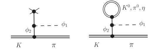
Figure 4: The contributions to the $K\to\pi\phi_{1}$ decay in Model 1 proportional to $\langle\phi_{2}\rangle$ (right), and the related one-loop tadpole diagram (left).

In order to simplify the discussion we assume below that the vacuum expectation values (vevs) of the scalar fields $\phi_{1,2}$ vanish, $\langle\phi_{1}\rangle=\langle\phi_{2}\rangle=0$. If this is not the case the $K\to\pi\phi_{1}$ decays receive additional GN-conserving contributions, see Fig. 4 (right). More precisely, it is the renormalised vevs that are set to zero, $\langle\phi_{1}\rangle_{\rm ren}=\langle\phi_{2}\rangle_{\rm ren}=0$, since we work to one loop order. That is, we set the sum of the two diagrams in Fig. 4 to be zero. Had we set them instead to their natural value, $\langle\phi_{i}\rangle_{\rm ren}\sim m_{K}g_{dd}^{(i)}/16\pi^{2}$, our results would not change qualitatively. While ${\cal M}(K^{+}\to\pi^{+}\phi_{1})$ would be modified by an ${\mathcal{O}}(1)$ factor, in ${\cal M}(K_{L}\to\pi^{0}\phi_{1})$ such contributions are always subleading and one would thus still have large violations of the GN bound.

3.1 Estimating the transition rates using ChPT

We use ChPT to calculate the transition rates. In constructing the ChPT we count $\phi_{1}\sim\phi_{2}\sim{\mathcal{O}}(p)$. As far as QCD is concerned $\phi_{1,2}$ are external sources and can be treated as spurions  Gasser and Leutwyler (1985); Pich (1995) when building the low energy effective Lagrangian. The QCD Lagrangian, including (6), can be conveniently rewritten as,

$$\begin{split}{\cal L}_{{\rm QCD}+\phi}=&\bar{q}(i\not{\partial}+g_{s}\not{G}^{a}T^{a})q-\bar{q}{\cal M}_{q}q-\sum_{i}\phi_{i}\,\bar{q}(\chi_{S}^{(i)}-i\chi_{P}^{(i)}\gamma_{5})q,\end{split}$$ (10)

where we keep only the light quarks, $q=(u,d,s)$. The diagonal mass matrix is ${\cal M}_{q}=\operatorname{diag}(m_{u},m_{d},m_{s})$, while $\chi_{S,P}^{(i)}$ are $3\times 3$ Hermitian matrices describing the quark couplings to $\phi_{1,2}$,

$$\big{[}\chi_{S}^{(i)}\big{]}_{qq^{\prime}}=-\frac{1}{2}\big{(}g^{(i)}_{qq^{\prime}}+g_{q^{\prime}q}^{(i)*}\big{)},\qquad\big{[}\chi_{P}^{(i)}\big{]}_{qq^{\prime}}=-\frac{i}{2}\big{(}g^{(i)}_{qq^{\prime}}-g_{q^{\prime}q}^{(i)*}\big{)}\;.$$ (11)

Since we set the couplings to the up quark to zero they have the following form

$$\chi_{S}^{(i)}=-\begin{pmatrix}0&0&0\\ 0&\operatorname{Re}g_{dd}^{(i)}&\bar{g}_{ds}^{(i)}\\ 0&\bar{g}_{sd}^{(i)}&\operatorname{Re}g_{ss}^{(i)}\end{pmatrix},\qquad\chi_{P}^{(i)}=\begin{pmatrix}0&0&0\\ 0&\operatorname{Im}g_{dd}^{(i)}&\hat{g}_{ds}^{(i)}\\ 0&\hat{g}_{sd}^{(i)}&\operatorname{Im}g_{ss}^{(i)}\end{pmatrix}.$$ (12)

The off-diagonal couplings in (12),

$$\bar{g}_{ds}^{(i)}=\bar{g}_{sd}^{(i)*}=\tfrac{1}{2}\big{(}g_{ds}^{(i)}+g_{sd}^{(i)*}\big{)},\qquad\hat{g}_{ds}^{(i)}=\hat{g}_{sd}^{(i)*}=-\tfrac{i}{2}\big{(}g_{ds}^{(i)}-g_{sd}^{(i)*}\big{)},$$ (13)

are the origin of the flavor violations.

The Lagrangian for QCD with the flavor violating $\phi_{1,2}$, ${\cal L}_{{\rm QCD}+\phi}$, is formally invariant under a global $SU(3)_{R}\times SU(3)_{L}$ transformation, $q_{R,L}\to g_{R,L}q_{R,L}$, provided $\chi_{S,P}^{(i)}\phi_{i}$ and ${\cal M}_{q}$ are promoted to spurions transforming as

$$s+ip \to g_{R}(s+ip)g_{L}^{\dagger},$$ (14)

where $s$ and $p$ stand for

$$s={\cal M}_{q}+\sum_{i}\chi_{S}^{(i)}\phi_{i},\,\qquad p=\sum_{i}\chi_{P}^{(i)}\phi_{i},$$ (15)

with $\chi_{S,P}^{(i)}$ given in (12).

The LO ChPT Lagrangian, with $\phi_{1,2}$ included as light degrees of freedom, is given by

$$\begin{split}{\cal L}_{{\rm ChPT}+\phi}^{(2)}&=\frac{f^{2}}{4}{\rm Tr}\big{(}\partial_{\mu}U\partial^{\mu}U^{\dagger}\big{)}+B_{0}\frac{f^{2}}{2}\operatorname{Tr}\big{[}(s-ip)U+(s+ip)U^{\dagger}\big{]}\\ &+\frac{1}{2}\partial_{\mu}\phi_{i}\partial^{\mu}\phi_{i}-\frac{m_{\phi_{i}}^{2}}{2}\phi_{i}^{2}+\lambda m_{S}\phi_{2}^{2}\phi_{1}+\cdots\;,\end{split}$$ (16)

where the ellipses stand for additional terms in the scalar potential. Here $U(x)=\exp(i\lambda^{a}\pi^{a}/f)$ is the unitary matrix parametrizing the meson fields Gasser and Leutwyler (1985); Pich (1995), $B_{0}$ is a constant related to the quark condensate, $B_{0}(\mu=2{\rm~{}GeV})=2.666(57)$ GeV, $f$ is related to the pion decay constant $f\simeq f_{\pi}/\sqrt{2}=92.2(1)$ MeV Aoki et al. (2019), with normalization $\langle 0|\bar{u}\gamma_{\mu}\gamma_{5}d(0)|\pi^{-}(p)\rangle=ip_{\mu}f_{\pi}$. The kaon decay constant $f_{K}=155.6\pm 0.4$ MeV Tanabashi et al. (2018) accommodates SU(3) breaking at times.

In this paper we work to partial NLO order: all LO terms in the chiral expansion ${\mathcal{O}}(p^{2})$ are kept, as well as the one loop corrections which are of order ${\mathcal{O}}(p^{4})$ and all finite. The complete ${\mathcal{O}}(p^{4})$-expressions for decay amplitudes involves additional contact terms (counter-terms or low energy constants), parametrically of the same size as the one loop corrections. However, since $\phi_{1,2}$ are propagating degrees of freedom in our EFT the values of the low energy constants in ${\mathcal{O}}(p^{4})$-ChPT are generally different from the ones in pure QCD and therefore unknown. The associated error in $K_{L}\to\pi^{0}\phi_{1}$ is small, since the NLO corrections are always subleading, while in $K^{+}\to\pi^{+}\phi_{1}$ they could give ${\mathcal{O}}(1)$ corrections but would not invalidate our conclusions. For simplicity they are set to zero throughout and we do not discuss them any further.

Next we calculate the $K\to\pi\phi_{1}$ decay amplitudes. Expanding in the meson fields the ${\mathcal{O}}(p^{2})$ Lagrangian reads

$$\begin{split}{\cal L}_{{\rm ChPT}+\phi}^{(2)}&\supset B_{0}f\sum_{i}\phi_{i}\Big{(}\sqrt{2}\hat{g}_{ds}^{(i)}\bar{K}^{0}+\sqrt{2}\hat{g}_{sd}^{(i)}K^{0}-\operatorname{Im}g_{dd}^{(i)}\pi^{0}+\tfrac{1}{\sqrt{3}}\operatorname{Im}\big{(}g_{dd}^{(i)}-2g_{ss}^{(2)}\big{)}\eta\Big{)}\\ &+B_{0}\sum_{i}\phi_{i}\Big{\{}\operatorname{Re}(g_{dd}^{(i)}+g_{ss}^{(i)})K^{0}\bar{K}^{0}+\operatorname{Re}(g_{dd}^{(i)})\big{(}\tfrac{1}{2}(\pi^{0})^{2}-\tfrac{1}{\sqrt{3}}\eta\pi^{0}\big{)}+\\ &\qquad+\operatorname{Re}g_{ss}^{(i)}K^{+}K^{-}+\operatorname{Re}g_{dd}^{(i)}\pi^{+}\pi^{-}+\\ &\qquad+\Big{[}\bar{g}_{sd}^{(i)}\big{(}-\tfrac{1}{\sqrt{2}}K^{0}\pi^{0}+K^{+}\pi^{-}-\tfrac{1}{\sqrt{6}}K^{0}\eta\big{)}+{\rm h.c.}\Big{]}+\cdots\Big{\}}\;,\end{split}$$ (17)

where we only kept terms relevant for the calculation of the $K\to\pi\phi_{1}$ transition, and the analysis of experimental bounds on the $\phi_{1}$-couplings.

The NP contributions to the decay amplitude for the $K_{L}\to\pi^{0}\phi_{1}$ and $K^{+}\to\pi^{+}\phi_{1}$ transitions are, see Fig. 3,

$$\begin{split}{\cal M}(K_{L}\to\pi^{0}\phi_{1})_{\rm NP}&=\biggr{\{}2\operatorname{Im}\hat{g}_{sd}^{(2)}\operatorname{Im}g_{dd}^{(2)}\Delta_{\phi_{2}}(m_{K}^{2})\Delta_{\phi_{2}}(m_{\pi}^{2})\lambda m_{S}B_{0}f_{K}f_{\pi}\\ &\qquad\quad+\operatorname{Im}\bar{g}_{sd}^{(1)}-\frac{\operatorname{Im}\bar{g}_{sd}^{(2)}}{8\pi^{2}}\lambda m_{S}B_{0}{\cal F}^{(2)}_{L}(I)\Big{\}}B_{0}\;,\end{split}$$ (18)

$${\cal M}(K^{+}\to\pi^{+}\phi_{1})_{\rm NP} =-\Big{\{}\bar{g}_{sd}^{(1)}-\frac{\bar{g}_{sd}^{(2)}}{8\pi^{2}}\lambda m_{S}B_{0}{\cal F}^{(2)}_{+}(I)\Big{\}}B_{0}\;,$$ (19)

where $\Delta_{X}(k^{2})\equiv 1/(k^{2}-m_{X}^{2})$ hereafter and

$${\cal F}^{(2)}_{L}(Y) =\operatorname{Re}g^{(2)}_{ss}Y(m_{K})+\operatorname{Re}g^{(2)}_{dd}\big{(}Y(m_{K})+Y(m_{\pi})-\tfrac{1}{3}Y(m_{\eta})\big{)}\;,$$ (20)

$${\cal F}^{(2)}_{+}(Y) =\operatorname{Re}g^{(2)}_{ss}Y(m_{K})+\operatorname{Re}g^{(2)}_{dd}Y(m_{\pi})\;,$$ (21)

are structures occurring in all three models. They depend on the loop function $I(m_{X})=C_{0}(m_{K}^{2},m_{\phi_{1}}^{2},m_{\pi}^{2},m_{X}^{2},m_{\phi_{2}}^{2},m_{\phi_{2}}^{2})$, with $C_{0}$ the standard scalar three-point Passarino-Veltman function (cf. App. B). In the $m_{\phi_{2}}\gg m_{K},m_{X}$ limit we have $I(m_{X})\to-1/m_{\phi_{2}}^{2}$. Moreover, the replacement $f^{2}\to f_{\pi}f_{K}/2$ accounts for the main SU(3) breaking effects.

Note that the amplitude vanishes in the limit of no CP violation, $\operatorname{Im}\hat{g}_{sd}^{(i)},\operatorname{Im}\bar{g}_{sd}^{(i)}\to 0$. The first term in (18), proportional to $\hat{g}_{sd}^{(2)}$, is the ${\mathcal{O}}(p^{2})$ contribution due to the tree level exchange of $\phi_{2}$, see the 3rd diagram in Fig. 3. It is isospin violating since it gives rise to the $K_{L}\to\pi^{0}\phi_{1}$ transition but not to $K^{+}\to\pi^{+}\phi_{1}$. The first term in the second line of Eq. (18) is the remaining ${\mathcal{O}}(p^{2})$ contribution, due to the emission of $\phi_{1}$ directly from the meson line, see the 1st diagram in Fig. 3. This contribution is isospin conserving – it is present for both $K_{L}\to\pi^{0}\phi_{1}$ and $K^{+}\to\pi^{+}\phi_{1}$ transitions. It is proportional to $\bar{g}_{sd}^{(1)}$ and is thus small due to the assumed hierarchy among the couplings, Eq. (7).

The hierarchy of couplings $|g_{sd,ds}^{(2)}|\gg|g_{sd,ds}^{(1)}|$ thus leads to maximal violation of the GN bound by NP contributions. However, this violation cannot be arbitrarily large. Even in the $\bar{g}_{sd}^{(1)}\to 0$ limit we still have isospin conserving NP contributions generated at one loop, see the 2nd diagram in Fig. 3, giving the last term in (18). If $\phi_{2}$ is heavy and integrated out these radiative corrections match onto the $\phi_{1}-K\pi$ vertex, which is then radiatively induced. Moreover the $K_{L}\to\pi^{0}\phi_{1}$ and $K^{+}\to\pi^{+}\phi_{1}$ decays receive contributions from $\pi^{0}-\phi_{1}$ mixing where flavor violation comes from the SM $K\to\pi\pi$ transition. For our choices of parameters these contributions are always negligible.

The NP contributions add coherently to the SM rate,

$$\Gamma(K_{L}\to\pi^{0}+{\rm inv})=\Gamma(K_{L}\to\pi^{0}\nu\bar{\nu})_{\rm SM}+\Gamma(K_{L}\to\pi^{0}\phi_{1})_{\rm NP},$$ (22)

and the partial decay width due to NP is

$$\Gamma(K_{L}\to\pi^{0}\phi_{1})_{\rm NP}=\frac{1}{8\pi}\big{|}{\cal M}(K_{L}\to\pi^{0}\phi_{1})_{\rm NP}|^{2}\frac{p_{\pi}}{m_{K}^{2}},$$ (23)

where $p_{\pi}=\lambda^{1/2}(m_{K}^{2},m_{\pi}^{2},m_{\phi_{1}}^{2})/(2m_{K})$ is the pion’s momentum in the $K_{L}$ rest frame and $\lambda(x,y,z)=x^{2}+y^{2}+z^{2}-2xy-2xz-2yz$ the kinematic Källén function. The expressions for the $K^{+}\to\pi^{+}+{\rm inv}$ decay is completely analogous. Numerically, this gives (the SM predictions are taken from Refs. Buras et al. (2005); Brod et al. (2011); Buras et al. (2015); Mescia and Smith (2007))

$$\begin{split}\text{Br}(K_{L}\to\pi^{0}+{\rm inv})&=\underbrace{(3.4\pm 0.6)\times 10^{-11}}_{{\rm SM}}\\ &+\underbrace{6.0\times 10^{-9}\,\biggr{(}\frac{\operatorname{Im}\hat{g}_{sd}^{(2)}}{5\cdot 10^{-9}}\biggr{)}^{2}\biggr{(}\frac{\operatorname{Im}g_{dd}^{(2)}}{10^{-3}}\biggr{)}^{2}\biggr{(}\frac{\lambda m_{S}}{1{\rm~{}GeV}}\biggr{)}^{2}\biggr{(}\frac{1{\rm~{}GeV}}{m_{\phi_{2}}}\biggr{)}^{8}}_{\rm NP},\end{split}$$ (24)

where we kept only the leading term for the NP contribution. The typical values of the inputs parameters for the NP contribution were chosen such that they reproduce roughly the KOTO anomaly (in fact slightly larger, but within $1\sigma$). Note the very high scaling in the $\phi_{2}$ mass, underscoring that $\phi_{2}$ needs to be relatively light in order to have large violations of the GN bound. For the charged kaon decay the numerical result is

$$\begin{split}{\rm Br}(K^{+}\to\pi^{+}+{\rm inv})=&\underbrace{(8.4\pm 1.0)\times 10^{-11}}_{{\rm SM}}+\underbrace{5.0\times 10^{-11}\biggr{|}\frac{\bar{g}_{sd}^{(1)}}{10^{-13}}\biggr{|}^{2}}_{\rm NP},\end{split}$$ (25)

where in the NP contribution we only kept the tree level term and set the value of $\bar{g}_{sd}^{(1)}$ to be similar to the one-loop threshold correction $\bar{g}_{sd}^{(1)}\sim\bar{g}_{sd}^{(2)}g_{dd}^{(2)}/8\pi^{2}$, cf. Eq. (19), with the typical values of the later couplings as in (24). While the correction to $K^{+}\to\pi^{+}+{\rm inv}$ is ${\mathcal{O}}(1)$ of the SM branching ratio, the correction to $K_{L}\to\pi^{0}+{\rm inv}$ can be orders of magnitude above the SM, giving large violations of the GN bound. Note that NP in Model 1 contributes to the 2-body decay $K^{+}\to\pi^{+}+X^{0}$ only, and for massless $X^{0}$ is subject to the bound $\text{Br}(K^{+}\to\pi^{+}+X^{0})<0.73\times 10^{-10}$ from E949 Adler et al. (2008), which is slightly stronger than the preliminary NA62 bounds on the 3-body decay $\text{Br}(K^{+}\to\pi^{+}+{\rm inv})_{\rm exp}<2.44\times 10^{-10}$ and the 2-body decay $\text{Br}(K^{+}\to\pi^{+}+X^{0})_{\rm exp}\lesssim 1.9\times 10^{-10}$ (for massless $X^{0}$) Volpe .

3.2 Constraints on $\hat{g}_{ds}^{(i)}$ from $K^{0}-\bar{K}^{0}$ mixing

The $K^{0}-\bar{K}^{0}$ mixing is an important constraint on the model. The contributions to the meson mixing matrix element are

$$\begin{split}M_{12}=M_{12}^{\rm SM}+M_{12}^{\rm NP}=&-\frac{1}{2m_{K}}\langle K^{0}|\mathcal{L}_{\rm eff}^{\rm SM}(0)|\bar{K}^{0}\rangle-\frac{i}{4m_{K}}\times\\ &\times\int d^{4}x\langle K^{0}|T{\mathcal{L}}_{{\rm ChPT}+\phi}^{(2)}(x),{\mathcal{L}}_{{\rm ChPT}+\phi}^{(2)}(0)\}|\bar{K}^{0}\rangle+\cdots,\end{split}$$ (26)

where the tree-level exchanges of $\phi_{2}$ is

$$\begin{split}M_{12}^{\rm NP}=-\frac{(\hat{g}_{ds}^{(2)}B_{0}f_{K})^{2}}{2m_{K}(m_{\phi_{2}}^{2}-m_{K}^{2})}+\cdots,\end{split}$$ (27)

with the ellipses denoting higher order terms (we also neglect the NP contributions to the absorptive mixing amplitude since it only enters at one loop). The replacement $f\to f_{K}/\sqrt{2}$ accounts for the SU(3) breaking.

We consider two constraints, $\Delta m_{K}$ and $\epsilon_{K}$ which are CP conserving and CP violating respectively. Using the relation $\Delta m_{K}=2{\rm Re}M_{12}$ and conservatively assuming, due to the relatively uncertain SM predictions of $\Delta m_{K}$, that the NP saturates the measured $\Delta m_{K}$, we obtain in the limit $m_{\phi_{2}}\gg m_{K}$,

$$\begin{split}\frac{\Delta m_{K}}{m_{K}}&\simeq 0.69\Big{|}\operatorname{Re}\Big{[}\big{(}\hat{g}_{ds}^{(2)}\big{)}^{2}\Big{]}\Big{|}\biggr{(}\frac{1{\rm~{}GeV}}{m_{\phi_{2}}}\biggr{)}^{2}\;,\end{split}$$ (28)

and with the experimental value $\Delta m_{K}^{\rm expt.}=3.484(6)\times 10^{-12}$ MeV Tanabashi et al. (2018), this translates to

$$\sqrt{\Big{|}\operatorname{Re}\Big{[}\big{(}\hat{g}_{ds}^{(2)}\big{)}^{2}\Big{]}\Big{|}}<1.0\cdot 10^{-7}\times\biggr{(}\frac{m_{\phi_{2}}}{1{\rm~{}GeV}}\biggr{)}\;.$$ (29)

To obtain the bounds on non-SM CP violating contributions to $K^{0}-\bar{K}^{0}$ mixing we use the normalized quantity

$$C_{\varepsilon_{K}}=\frac{|\epsilon_{K}^{{\rm SM}+a}|}{|\epsilon_{K}^{\rm SM}|}\;.$$ (30)

For the theoretical prediction of $\epsilon_{K}$ we use the expression Buras et al. (2010)

$$\epsilon_{K}=e^{i\phi_{\epsilon}}\sin\phi_{\epsilon}\biggr{(}\frac{\operatorname{Im}M_{12}}{\Delta m_{K}}+\xi\biggr{)}\;,$$ (31)

where

$$\xi\simeq\frac{\operatorname{Im}\Gamma_{12}}{\Delta\Gamma_{K}}\;.$$ (32)

We take the values for $\Delta m_{K}=m_{L}-m_{S}$, $\Delta\Gamma_{K}=\Gamma_{S}-\Gamma_{L}$, and $\phi_{\epsilon}=\arctan(2\Delta m_{K}/\Delta\Gamma_{K})$ from experiment Tanabashi et al. (2018). With the SM prediction for $|\epsilon_{K}|$ from Brod et al. (2019), and the NP contribution to $M_{12}$, $\Gamma_{12}$ from Eq. (27) we get

$$\begin{split}\delta C_{\epsilon_{K}}=C_{\epsilon_{K}}-1&=-5.8\times 10^{16}\,\operatorname{Im}\big{[}(\hat{g}_{ds}^{(2)})^{2}\big{]}\biggr{(}\frac{1{\rm~{}GeV}}{m_{\phi_{2}}}\biggr{)}^{2},\end{split}$$ (33)

The global CKM fit by the UTFit collaboration results in $0.87<C_{\epsilon_{K}}<1.39$ at 95% CL Bona et al. (2008); Collaboration , which translates to the following $1\sigma$ bounds

$$-(2.6\times 10^{-9})^{2}\biggr{(}\frac{m_{\phi_{2}}}{1{\rm~{}GeV}}\biggr{)}^{2}<\operatorname{Im}\big{[}(\hat{g}_{ds}^{(2)})^{2}\big{]}<(1.5\times 10^{-9})^{2}\biggr{(}\frac{m_{\phi_{2}}}{1{\rm~{}GeV}}\biggr{)}^{2}.$$ (34)

These bounds will improve in the future, once the improved prediction for $\epsilon_{K}$ Brod et al. (2019) is implemented in the global CKM fits.

3.3 Constraints from $\epsilon^{\prime}/\epsilon$

The tree level exchanges of $\phi_{2}$ contribute to $K\to\pi\pi$ decays. These contributions can be CP violating and can thus contribute to $\epsilon^{\prime}/\epsilon$. In general, the matrix elements can be decomposed into isospin amplitudes $A_{I}$ of the final state pions $|(\pi\pi)_{I}\rangle$. The latter read, with appropriate Clebsch-Gordan coefficients for our chiral Lagrangian D’Ambrosio and Isidori (1998),

$${\cal M}(K^{0}\to\pi^{+}\pi^{-}) \;=\; A_{0}+\frac{1}{\sqrt{2}}A_{2}\;,$$

$${\cal M}(K^{0}\to\pi^{0}\pi^{0}) \;=\; A_{0}-{\sqrt{2}}A_{2}\;,$$

$${\cal M}(K^{+}\to\pi^{+}\pi^{0}) \;=\; \phantom{A_{0}+\;\;\;\;}\frac{3}{2}A_{2}\;.$$ (35)

In terms of these amplitudes the real part of ${\epsilon^{\prime}}/{\epsilon}$ assumes the form

$$\operatorname{Re}\left(\frac{\epsilon^{\prime}}{\epsilon}\right)=-\frac{\omega}{\sqrt{2}|\epsilon_{K}|}\biggr{[}\frac{\operatorname{Im}A_{0}}{\operatorname{Re}A_{0}}-\frac{\operatorname{Im}A_{2}}{\operatorname{Re}A_{2}}\biggr{]}\;,$$ (36)

where $\omega\equiv\operatorname{Re}A_{2}/\operatorname{Re}A_{0}$. In our model, the isospin amplitudes are easily obtained from (3.3) through an emission and $s$-channel tree level diagram

$$A_{2} =-\frac{2}{3}B_{0}^{2}f\bar{g}_{sd}^{(2)}\operatorname{Im}g_{dd}^{(2)}\Delta_{\phi_{2}}(m_{\pi}^{2}),$$ (37)

$$A_{0} =\sqrt{2}B_{0}^{2}f\hat{g}_{sd}^{(2)}\operatorname{Re}g_{dd}^{(2)}\Delta_{\phi_{2}}(m_{K}^{2})-\frac{1}{\sqrt{2}}A_{2}\;.$$ (38)

Using the measured values, $\operatorname{Re}A_{0}=27.04(1)\times 10^{-8}$ GeV, $\operatorname{Re}A_{2}=1.210(2)\times 10^{-8}$ GeV Cirigliano et al. (2012), $\omega^{-1}=22.2(1)$ D’Ambrosio and Isidori (1998), $|\epsilon_{K}|=(2.10^{+0.27}_{-0.20})\cdot 10^{-3}$ Charles et al. (2005), our model then affects the imaginary parts of the isospin amplitudes and leads to the following shift

$$\operatorname{Re}\left(\frac{\epsilon^{\prime}}{\epsilon}\right)_{\rm BSM}=2\times 10^{-3}\biggr{[}0.04\biggr{(}\frac{\operatorname{Im}\hat{g}_{sd}^{(2)}}{10^{-9}}\biggr{)}\biggr{(}\frac{\operatorname{Re}g_{dd}^{(2)}}{10^{-3}}\biggr{)}+0.32\biggr{(}\frac{\operatorname{Im}\bar{g}_{sd}^{(2)}}{10^{-9}}\biggr{)}\biggr{(}\frac{\operatorname{Im}g_{dd}^{(2)}}{10^{-3}}\biggr{)}\biggr{]}\;,$$ (39)

with $m_{\phi_{2}}=1\;\text{GeV}$ for reference. For brevity we used the central values of the inputs above. This is to be compared with the experimental value $\operatorname{Re}(\epsilon^{\prime}/\epsilon)_{\rm exp}=(16.6\pm 2.3)\times 10^{-4}$ Tanabashi et al. (2018) and the SM prediction from lattice QCD, $\operatorname{Re}(\epsilon^{\prime}/\epsilon)_{\rm RBC-UKQCD}=(21.7\pm 8.4)\times 10^{-4}$ Abbott et al. (2020), which gives the 95 % C.L. for the positive BSM contributions to be $\operatorname{Re}(\epsilon^{\prime}/\epsilon)_{\rm BSM}<2.2\times 10^{-3}$ (alternative treatments of lattice QCD inputs as well as isospin breaking effects can lead to somewhat stronger bounds $\operatorname{Re}(\epsilon^{\prime}/\epsilon)_{\rm BSM}<1.3(7)\times 10^{-3}$ based on octet (nonet) schemes Aebischer et al. (2020)).

3.4 Constraints on representative benchmarks

To highlight the typical values of couplings that can lead to sizable correction in $K\to\pi+$ inv decays, while passing all other constraints, we form a benchmark 1 (BM1) and a benchmark 2 (BM2),

$${\rm\bf BM~{}1:}\qquad g_{dd}^{(2)} \;=\; \tfrac{(1+i)}{\sqrt{2}}g_{dd}\;,\quad \bar{g}_{sd}^{(2)}\;=\;\hat{g}_{sd}^{(2)}=\tfrac{(1+i)}{\sqrt{2}}g_{sd}\;,$$ (40)

$${\rm\bf BM~{}2:}\qquad g_{dd}^{(2)} \;=\; ig_{dd}\;,\quad \bar{g}_{sd}^{(2)}\;=\;0\;,\quad\hat{g}_{sd}^{(2)}=ig_{sd}\;.$$ (41)

These depend on two real parameters, $g_{dd}$ and $g_{sd}$, parametrizing couplings of $\phi_{2}$ to quarks. All the remaining couplings of $\phi_{2}$ to quarks as well as all the direct couplings of $\phi_{1}$ to quarks are set to zero in accordance with previous discussions. The triple scalar coupling is fixed to $\lambda_{S}m_{S}=1{\rm~{}GeV}$ (and other potentially relevant scalar couplings assumed to be small, see Section 3.5.1). The mass of $\phi_{1}$ is taken to be small, $m_{\phi_{1}}=1$ MeV, while $m_{\phi_{2}}$ is kept as a free parameter that is varied in the range $m_{\phi_{2}}\in[0.4,1.5]$ GeV, cf. footnote 2.

The form of couplings in BM1, Eq. (40), is such that the NP contributions to $\epsilon_{K}$ are maximized. This benchmark is thus representative of the parameter space that is most constrained. Fixing $g_{dd}=10^{-3}$ the allowed regions are shown in Fig. 5. The red regions are excluded by the NA62 bound on $\text{Br}(K^{+}\to\pi^{+}\phi_{1})_{\rm exp}\lesssim 1.9\times 10^{-10}$ Volpe , the E949 bound $\text{Br}(K^{+}\to\pi^{+}\phi_{1})_{\rm exp}<0.73\times 10^{-10}$ Adler et al. (2008) and by the KOTO bound $\text{Br}(K_{L}\to\pi^{0}\phi_{1})<2.4\times 10^{-9}$ Ahn et al. (2019). The E949 and NA62 bounds shown are for massless $\phi_{1}$, which is a good approximation for our benchmarks, where $m_{\phi_{1}}=1$ MeV. For heavier masses, above $m_{\pi}$, the bound is expected to become significantly weaker and completely disappear for $m_{\phi_{1}}\simeq m_{\pi^{0}}$, as in Artamonov et al. (2009). The green bands denote the $1\sigma$ bands of the branching ratio $\text{Br}(K_{L}\to\pi^{0}+{\rm inv})_{\rm KOTO}=\big{(}2.1^{+2.0}_{-1.1}\big{)}\times 10^{-9}$ Shinohara ; Kitahara et al. (2020) that corresponds to the anomalous KOTO events. The blue line denotes the GN bound, showing that large violations of the GN bound are possible in this model.

This violation is most apparent in Fig. 5 (right) which gives the allowed values of $g_{sd}$ as a function of $m_{\phi_{2}}$, with the dashed lines denoting contours of the ratio $\text{Br}(K_{L}\to\pi^{0}+{\rm inv})/\text{Br}(K^{+}\to\pi^{+}+{\rm inv})$. The present KOTO bound is saturated by values for this ratio of around 20, while still satisfying the $\epsilon_{K}$ constraint, Eq. (34), and the $\pi^{0}\to{\rm inv}$ constrain discussed below, see Eq. (44). The excluded regions are shown hatched in Fig. 5 (right). The bound from $\operatorname{Re}(\epsilon^{\prime}/\epsilon)$, Eq. (39), is less stringent and not displayed as there is already a lot of information in the figure. It is straightforward to plot this constraint from the formulae given in Section3.3.

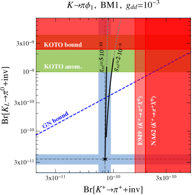
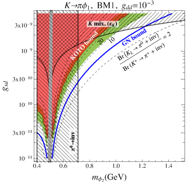
Figure 5: The parameter space for Model 1, BM1, for $g_{dd}=10^{-3}$ in (40). The GN bound is denoted with blue lines, while the green regions give the $1\sigma$ bands corresponding to KOTO anomalous events Kitahara et al. (2020); Shinohara . Left: the predictions for $\text{Br}(K^{+}\to\pi^{+}+{\rm inv})$, $\text{Br}(K_{L}\to\pi^{0}+{\rm inv})$, varying $m_{\phi_{2}}\in[0.4,1.5]$ GeV and for two values of $g_{sd}$ (black lines). The values closest to the SM (black cross) are reached for $m_{\phi_{2}}=1.5$ GeV. Blue regions are the 1$\sigma$ SM prediction bands, with the central values denoted by the dashed lines and a star, red regions are excluded by NA62 Ruggiero , E949 Adler et al. (2008) and KOTO Ahn et al. (2019). Right: Contours of $\text{Br}(K_{L}\to\pi^{0}+{\rm inv})/\text{Br}(K^{+}\to\pi^{+}+{\rm inv})$ (dashed lines) as functions of $g_{sd}$, $m_{\phi_{2}}$, with the hatched regions excluded by $K^{0}-\bar{K}^{0}$ mixing and $\pi^{0}\to inv$ bounds. The region around the kaon mass is masked out (gray region).

The solid black lines in Fig. 5 (left) show the values of $\text{Br}(K_{L}\to\pi^{0}+{\rm inv})$ and $\text{Br}(K^{+}\to\pi^{+}+{\rm inv})$ for $g_{sd}=5\cdot 10^{-10}$ and $g_{sd}=2\cdot 10^{-9}$, varying $m_{\phi_{2}}\in[0.4,1.5]$ GeV, while fixing $g_{dd}=10^{-3}$ (the grey dotted parts of the lines are excluded by a combination of $K^{0}-\bar{K}^{0}$ and $\pi^{0}\to$ inv constraints). The SM predictions for the two branching ratios, $\text{Br}(K^{+}\to\pi^{+}\nu\bar{\nu})_{\rm SM}=(8.4\pm 1.0)\times 10^{-11}$ and $\text{Br}(K_{L}\to\pi^{0}\nu\bar{\nu})_{\rm SM}=(3.4\pm 0.6)\times 10^{-11}$  Buras et al. (2005); Brod et al. (2011); Buras et al. (2015), are denoted with blue bands ($1\sigma$ ranges). For the larger value, $g_{sd}=2\cdot 10^{-9}$, the prediction is still quite far away from the SM for $m_{\phi_{2}}=1.5$ GeV, but would of course tend to the SM for $m_{\phi_{2}}\to\infty$. For larger values of $g_{sd}$ deviations from the SM prediction for $\text{Br}(K^{+}\to\pi^{+}+{\rm inv})$ at the level of a few are predicted for this benchmark and subject to the indicated constraints from E949, while for smaller values of $g_{sd}$ the deviations in $\text{Br}(K^{+}\to\pi^{+}+{\rm inv})$ become negligibly small. That is, it is possible to explain the KOTO anomalous events without having any appreciable NP effects in the charged kaon decay nor in $K^{0}-\bar{K}^{0}$ mixing.

We next move to BM2. The form of couplings in Eq. (41) was deliberately chosen such that there is no NP CP violation in $K^{0}-\bar{K}^{0}$ mixing, in order to avoid the $\epsilon_{K}$ bound. The bound from $\Delta m_{K}$, Eq. (29), on CP conserving contributions to $K^{0}-\bar{K}^{0}$ mixing is much weaker, giving the hatched excluded region in Fig. 6 (right). This means that for the same mass of $\phi_{2}$ the flavor violating couplings to quarks can be much larger than in BM1. In Fig. (right) 6 we show the $g_{dd}=3\times 10^{-5}$ slice of the parameter space, in which case $g_{sd}$ can be as large as $10^{-7}$. Furthermore, the form of couplings in BM2, Eq. (41), is such that there is no NP effect at all in $\text{Br}(K^{+}\to\pi^{+}+{\rm inv})$, to the order we are working, and the E949 bound is completely avoided. In contrast, the effect on $\text{Br}(K_{L}\to\pi^{0}+{\rm inv})$ can be very large and easily saturate KOTO’s present upper bound, as shown for two representative couplings $g_{sd}=3\times 10^{-9},8\times 10^{-8}$ (black lines, with dashed parts of the lines excluded by $\Delta m_{K}$). BM2 comes with enhanced symmetry; $\phi_{2}$ is a pure pseudoscalar and $\phi_{1}$ a pure scalar. This has implications for flavor conserving couplings of $\phi_{1}$, to which we turn next.

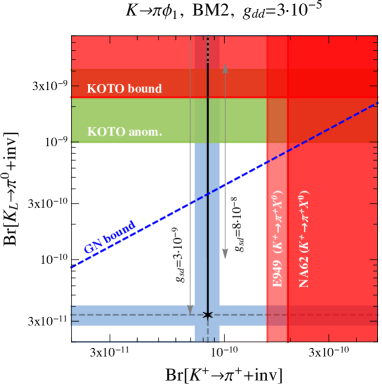
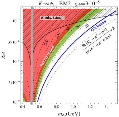
Figure 6: The preferred parameter space for Model 1, BM2. Color coding is the same as in Fig. 5. See end of Section 3.4 for comments on these figures.

3.5 Constraints on the $\phi_{1}$-couplings

So far the scalar mass $\phi_{1}$ has been fixed to $1$ MeV. Next, we show that for the two benchmarks the radiatively generated couplings of $\phi_{1}$ to pions, nucleons, and photons are all well below the bounds for a large range of $\phi_{1}$ masses (including $m_{\phi_{1}}=1$ MeV). Figs. 5 and 6 are thus valid for a larger set of $\phi_{1}$ masses, as long as $m_{\phi_{1}}\ll m_{K}$.

3.5.1 Invisible pion decays

If kinematically allowed, $\pi^{0}\to\phi_{1}\phi_{1}$ can be an important phenomenological constraint. In Model 1 this decay can proceed through $\phi_{2}-\pi^{0}$ mixing though the loop diagram shown in Fig. 12 (left). In the $m_{\phi_{2}}\gg m_{\pi,\eta}$ limit the decay amplitude is

$${\cal M}(\pi^{0}\to\phi_{1}\phi_{1})=\frac{1}{12\pi^{2}}\frac{(\lambda m_{S})^{2}B_{0}^{2}f}{m_{\phi_{2}}^{4}}\operatorname{Re}g_{dd}^{(2)}\left(2\operatorname{Im}g_{dd}^{(2)}-\operatorname{Im}g_{ss}^{(2)}\right)\,.$$ (42)

The corresponding width is given by

$$\Gamma(\pi^{0}\to\phi_{1}\phi_{1})=\frac{|{\cal M}|^{2}}{32\pi m_{\pi}}\beta_{\phi_{1}}\,,$$ (43)

where here $\beta_{\phi_{1}}\equiv\big{(}1-4m_{\phi_{1}}^{2}/m_{\pi}^{2}\big{)}^{1/2}$, so that in the limit $m_{\phi_{1}}\ll m_{\pi}\ll m_{\phi_{2}}$, one has for the branching ratio (setting $\operatorname{Im}g_{ss}^{(2)}=0$ for simplicity)

$$\text{Br}(\pi^{0}\to\phi_{1}\phi_{1}) =1.2\times 10^{-9}\left(\frac{\operatorname{Re}g_{dd}^{(2)}}{10^{-3}}\right)^{2}\left(\frac{\operatorname{Im}g_{dd}^{(2)}}{10^{-3}}\right)^{2}\left(\frac{\lambda\,m_{S}}{\text{GeV}}\right)^{4}\left(\frac{\text{GeV}}{m_{\phi_{2}}}\right)^{8}\,.$$ (44)

The preliminary 90% C. L. experimental bound reported very recently by NA62 Volpe

$$\text{Br}(\pi^{0}\to\phi_{1}\phi_{1})<4.4\times 10^{-9}\,,$$ (45)

improves the E949 bound of $2.7\times 10^{-7}$ Artamonov et al. (2005) by almost two orders of magnitude. BM2 obeys this bound trivially, since $\pi^{0}\to\phi_{1}\phi_{1}$ if forbidden by parity ($\operatorname{Re}g_{dd}^{(2))}=0$). For BM1, on the other hand, the bound on ${\rm Br}(\pi^{0}\to{\rm inv})$, Eq. (45), represents a stringent constraint, as shown in Fig. 5 (right).

Finally, the $\pi^{0}\to\phi_{1}\phi_{1}$ decay could also proceed at tree level via an additional interaction term in (16) of the form $\delta{\cal L}=\lambda^{\prime}m_{S}\phi_{2}\phi_{1}^{2}$. Whereas, contrary to Model 2, $\lambda^{\prime}$ plays no role in the $K\to\pi\phi_{1}$ decays per se, it is potentially dangerous for the invisible pion decay. In the absence of a UV completion we may choose its initial value to be sufficiently small (zero in practice) to pass the constraint.

3.5.2 $\phi_{1}-\pi^{0}$ mixing

The $\phi_{i}$ mix with light pseudoscalars through the $g_{qq^{\prime}}^{(i)}$ couplings, Eq. (6). The $\phi_{1}-\pi^{0}$ part of the mass matrix to one loop receives contributions in Fig. 7, and is parametrized by the Lagrangian, $m_{\phi_{2}}\gg m_{\phi_{1},\pi,\eta}$,

$${\cal L}_{\rm eff}\supset-g_{1\pi}B_{0}f\phi_{1}\pi^{0},$$ (46)

with the effective $\phi_{1}-\pi^{0}$ coupling given by

$$\begin{split}g_{1\pi}&=\operatorname{Im}g_{dd}^{(1)}+\frac{1}{8\pi^{2}}\biggr{(}\frac{\lambda m_{S}B_{0}}{m_{\phi_{2}}^{2}}\biggr{)}\biggr{\{}\operatorname{Im}g_{dd}^{(2)}\operatorname{Re}g_{dd}^{(2)}L(m_{\pi})\\ &+\frac{1}{3}\left(\operatorname{Im}g_{dd}^{(2)}-2\operatorname{Im}g_{ss}^{(2)}\right)\operatorname{Re}g_{dd}^{(2)}L(m_{\eta})+\left(\overline{g}^{(2)}_{ds}\hat{g}^{(2)}_{sd}+{\rm h.c.}\right)L(m_{K})\biggr{\}}\;,\end{split}$$ (47)

where we have exceptionally kept the $g^{(2)}_{ds}$-terms since they are leading in BM2. The first term is due to tree level mixing, see Fig. 7 (left), the second term are the one loop corrections due to diagram in Fig. 7 (right). The loop function $L(m_{X})\equiv-m_{\phi_{2}}^{2}C_{0}(0,0,0,m_{X}^{2},m_{\phi_{2}}^{2},m_{\phi_{2}}^{2})$ is normalized such that $L(m_{X})\to 1$ for $m_{\phi_{2}}\gg m_{X}$. In the following we will take for simplicity this limit, which provides a reasonable approximation for the parameter region of interest, since $L_{\pi}\simeq 0.8,L_{K,\eta}\simeq 0.4$ for $m_{\phi_{2}}=400$ MeV. In the two benchmarks (40), (41), the effective $\phi_{1}-\pi^{0}$ couplings are

$${\bf BM~{}1}:\qquad g_{1\pi}^{\rm BM1} =2.3\times 10^{-8}\left(\frac{g_{dd}}{10^{-3}}\right)^{2}\left(\frac{\text{GeV}}{m_{\phi_{2}}}\right)^{2}\,,$$ (48)

$${\bf BM~{}2}:\qquad g_{1\pi}^{\rm BM2} =0\;.$$ (49)

In BM2 there is no $\phi_{1}-\pi^{0}$ mixing $\phi_{1}$ is a pure scalar and parity is conserved.

Working in the mass insertion approximation for the off-diagonal mass term, Eq. (46), the $\phi_{1}-\pi^{0}$ mixing angle, $s_{\theta}\equiv\sin\theta\approx\theta$, between the interaction states $\phi_{1}$ and the mass eigenstate $\phi_{1}^{\prime}\approx\phi_{1}-s_{\theta}\pi^{0}$ is

$$s_{\theta}=\frac{B_{0}f}{m_{\pi}^{2}-m_{\phi_{1}}^{2}}\,g_{1\pi}\,.$$ (50)

Note that this expression for the mixing angle is only valid for $m_{\phi_{1}}$ sufficiently far away from $m_{\pi}$. For the two benchmarks, we have

$${\bf BM~{}1}:\qquad s_{\theta}^{\rm BM1} =3.0\times 10^{-7}\left(\frac{g_{dd}}{10^{-3}}\right)^{2}\left(\frac{\text{GeV}}{m_{\phi_{2}}}\right)^{2}\,,$$ (51)

$${\bf BM~{}2}:\qquad s_{\theta}^{\rm BM2} =0\;.$$ (52)

The $\phi_{1}-\pi^{0}$ mixing is thus very small in most of the viable parameter space, justifying the use of the mass insertion approximation.

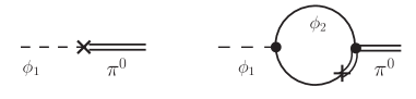
Figure 7: The leading order and one loop induced $\phi_{1}-\pi^{0}$ mixing.

3.5.3 Couplings of $\phi_{1}$ to photons

The dominant decay channel of $\phi_{1}$ is to two photons. In the limit $m_{\phi_{1}}\ll m_{\pi}$ the interactions with two photons are described by the effective Lagrangian

$${\cal L}_{\rm eff}\supset-\frac{1}{8}g_{1\gamma\gamma}\phi_{1}F^{\mu\nu}F^{\rho\sigma}\epsilon_{\mu\nu\rho\sigma}-\frac{1}{4}h_{1\gamma\gamma}\phi_{1}F^{\mu\nu}F_{\mu\nu}\;.$$ (53)

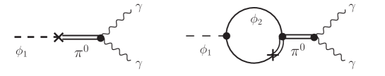
Figure 8: CP violating contributions to $\phi_{1}\to\gamma\gamma$, matching onto the coupling $g_{1\gamma\gamma}$.

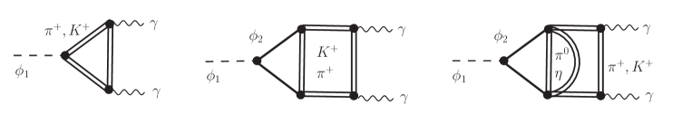
Figure 9: CP conserving contributions to $\phi_{1}\to\gamma\gamma$, matching onto the coupling $h_{1\gamma\gamma}$.

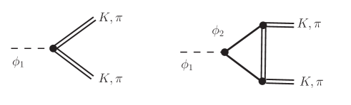
Figure 10: Tree level and one loop contributions matching onto the effective couplings $g_{1\pi\pi}$/$g_{1KK}$.

The dominant contribution to the CP violating coupling $g_{1\gamma\gamma}$ is from the $\pi^{0}$ anomaly term via the $\phi_{1}-\pi^{0}$ mixing, see Fig. 8. Working in the mass insertion approximation for the off-diagonal mass term, Eq. (46), gives

$$g_{1\gamma\gamma}=s_{\theta}\frac{\sqrt{2}\alpha}{\pi f_{\pi}}\approx g_{1\pi}\frac{6.2\times 10^{-3}\,\text{GeV}}{m_{\pi}^{2}-m_{\phi_{1}}^{2}}\xrightarrow{m_{\phi_{1}}\ll m_{\pi}}g_{1\pi}\,0.34\text{GeV}^{-1}\,,$$ (54)

with $g_{1\pi}$ given in (47).

The CP conserving $h_{1\gamma\gamma}$ coupling receives the first relevant contributions from radiative corrections with $K^{+}$ and $\pi^{+}$ running in the loop cf. Fig. 9. For our benchmarks the first nonzero contributions arises at two loops, while for BM2 the numerically most important contribution arises at three loops

$$h_{1\gamma\gamma}=h_{1\gamma\gamma}^{\rm 1+2\,loop}+h_{1\gamma\gamma}^{\rm 3\,loop}\,.$$ (55)

In the $m_{\phi_{2}}\gg m_{K}$ ($m_{\pi}\gg m_{\phi_{1}}$ by assumption) limit the one and two loop contributions, in Fig. 9, assume the form

$$h_{1\gamma\gamma}^{\rm 1+2\,loop}=\frac{\alpha}{12\pi}\left(\frac{g_{1\pi\pi}}{m_{\pi}^{2}}+\frac{g_{1KK}}{m_{K}^{2}}\right)\;,$$ (56)

whereas the effective couplings of $\phi_{1}$, ${\cal L}_{\rm eff}\supset\phi_{1}\left(g_{1\pi\pi}\pi^{+}\pi^{-}+g_{1KK}K^{+}K^{-}\right)$, to two light charged mesons evaluate to

$$g_{1\pi\pi}=B_{0}\biggr{[}\operatorname{Re}g_{dd}^{(1)}+\frac{\lambda B_{0}m_{S}}{8\pi^{2}m_{\phi_{2}}^{2}}\left((\operatorname{Re}g_{dd}^{(2)})^{2}+|\overline{g}_{sd}^{(2)}|^{2}\right)\biggr{]}\;,$$ (57)

and $g_{1KK}=g_{1\pi\pi}|_{dd\to ss}$. The first term in (57) is the tree level term from (17), see Fig. 10 (left). In both benchmarks, BM1 and BM2, this contribution was set to zero. The second term in (57) is the one loop correction, see Fig. 10 (right). We kept the flavor violating contribution proportional to $\bar{g}_{sd}$ even though it is numerically negligible.

For the three loop contribution to $h_{1\gamma\gamma}$ we resort to a NDA estimate, still in the $m_{\phi_{2}}\gg m_{K}$ limit,

$$h_{1\gamma\gamma}^{\rm 3\,loop}\approx\frac{\alpha}{4\pi}\frac{\lambda m_{S}}{(16\pi^{2})^{2}}\Big{(}\frac{B_{0}}{fm_{\phi_{2}}}\Big{)}^{2}\Big{[}\big{(}\operatorname{Im}g_{dd}^{(2)}\big{)}^{2}+{\mathcal{O}}(1)\times(\operatorname{Im}g_{ss}^{(2)})^{2}+{\mathcal{O}}(1)\times(\operatorname{Im}g_{dd}^{(2)})(\operatorname{Im}g_{ss}^{(2)})\Big{]}\;,$$

where the ${\mathcal{O}}(1)$ factors are not displayed.

Finally we are in a position to assemble the results for the benchmarks. Using $g_{sd}\ll g_{dd}$, the $\phi_{1}$–photon couplings evaluate to

$$\begin{split}{\bf BM1:}~{}~{}~{}g_{1\gamma\gamma}^{\rm BM1}&\simeq\frac{7.7\times 10^{-9}}{\text{GeV}}\left(\frac{g_{dd}}{10^{-3}}\right)^{2}\left(\frac{\text{GeV}}{m_{\phi_{2}}}\right)^{2}\,,\\ ~{}~{}~{}h_{1\gamma\gamma}^{\rm BM1}&\simeq\frac{4.8\times 10^{-10}}{\text{GeV}}\left(\frac{g_{dd}}{10^{-3}}\right)^{2}\left(\frac{\text{GeV}}{m_{\phi_{2}}}\right)^{2}\,,\end{split}$$ (58)

in BM1, while for BM2 they turn out to be

$$\begin{split}{\bf BM2:}~{}~{}~{}g_{1\gamma\gamma}^{\rm BM2}&=0\;,\\ ~{}~{}~{}h_{1\gamma\gamma}^{\rm BM2}&\sim\frac{2\times 10^{-14}}{\text{GeV}}\left(\frac{g_{dd}}{3\times 10^{-5}}\right)^{2}\left(\frac{\text{GeV}}{m_{\phi_{2}}}\right)^{2}\;,\end{split}$$ (59)

and we remind the reader that $\lambda m_{S}=1$ GeV for reference. The $g_{1\gamma\gamma}$ coupling vanishes in BM2 since $\phi_{1}$ is a parity even scalar in that benchmark. The value quoted for $h_{1\gamma\gamma}^{\rm BM2}$ is the NDA estimate of the flavor conserving 3 loop contribution. For representative values of $g_{dd}$ in the two benchmarks we used the values in Figs. 5 and Fig. 6 for BM1 and BM2, respectively.

The above couplings of $\phi_{1}$ to photons are sufficiently small that for both benchmarks the $\phi_{1}$ is stable on collider scales. More concretely, the $\phi_{1}\to\gamma\gamma$ partial decay width is given by

$$\Gamma_{1\gamma\gamma} =\frac{1}{64\pi}\big{(}g_{1\gamma\gamma}^{2}+h_{1\gamma\gamma}^{2}\big{)}m_{\phi_{1}}^{3}\,,$$ (60)

and this translates to

$${\bf BM1:~{}~{}}c\tau_{1\gamma\gamma}^{\rm BM1} =7\times 10^{11}\,{\rm m}\left(\frac{\text{MeV}}{m_{\phi_{1}}}\right)^{3}\left(\frac{10^{-3}}{g_{dd}}\right)^{4}\left(\frac{m_{\phi_{2}}}{\text{GeV}}\right)^{4},\,$$ (61)

$${\bf BM2:~{}~{}}c\tau_{1\gamma\gamma}^{\rm BM2} \sim 10^{23}\,{\rm m}\left(\frac{\text{MeV}}{m_{\phi_{1}}}\right)^{3}\left(\frac{3\times 10^{-5}}{g_{dd}}\right)^{4}\left(\frac{m_{\phi_{2}}}{\text{GeV}}\right)^{4},$$ (62)

such that $\phi_{1}$ is stable on solar to cosmological timescales. For such small couplings the laboratory constraints from, e.g., $\pi^{+}\to\phi_{1}e^{+}\nu$ decays Altmannshofer et al. (2019) are irrelevant, whereas astrophysical and cosmological constraints are important (cf. figure 1 in Ref. Jaeckel and Spannowsky (2016)) and further discussed in Section 3.5.5.

3.5.4 Couplings of $\phi_{1}$ to nucleons

The couplings of $\phi_{1}$ to protons and neutrons are tree-level and loop-level induced by $g_{dd}^{(1)}$ and $g_{dd}^{(2)}$ respectively, cf. Fig. 11. One can use Heavy Baryon Chiral Perturbation Theory (HBChPT) Jenkins and Manohar (1991) to organize different contributions. We only keep only the leading terms which are (in relativistic notation)

$${\cal L}=\frac{g_{A}}{f}(\bar{N}\gamma^{\mu}\gamma_{5}t^{a}N)\partial_{\mu}\pi^{a}+\sum_{i}(\bar{N}Y_{i}^{N}N)\phi_{i}+\cdots,$$ (63)

with $t^{a}=\sigma^{a}/2$, $a=1,2,3$ and $\sigma^{a}$ are Pauli matrices, $N=(p,n)$ the isospin doublet of nucleons, and

$$Y_{i}^{N}=\begin{pmatrix}\sum_{q}\operatorname{Re}(g_{qq}^{(i)}){\sigma_{q}^{p}}/{m_{q}}&0\\ 0&\sum_{q}\operatorname{Re}(g_{qq}^{(i)}){\sigma_{q}^{n}}/{m_{q}}\end{pmatrix},$$ (64)

the coupling between $\phi_{i}$ and nucleons with summation over $q=d,s$ (by assumption the couplings of $\phi_{1,2}$ to up quarks are zero). For the matrix elements of the scalar current, $\sigma_{q}^{N}\bar{u}_{N}u_{N}=\langle N|m_{q}\bar{q}q|N\rangle$ we use the values from Bishara et al. (2017), $\sigma_{d}^{p}=(32\pm 10){\rm~{}MeV},\sigma_{d}^{n}=(36\pm 10){\rm~{}MeV},\sigma_{s}^{p}=\sigma_{s}^{n}=(41.3\pm 7.7){\rm~{}MeV}$, along with the quark masses at $\mu=2$ GeV, $m_{d}=4.67(33)$ MeV, $m_{s}=93(8)$ MeV, while $g_{A}=1.2723(23)$ Tanabashi et al. (2018).

In the heavy $\phi_{2}$ limit the following effective Lagrangian

$$\begin{split}{\cal L}_{\rm eff}&=g_{1NN}m_{N}\phi_{1}(\bar{N}N)+2\tilde{g}_{1NN}m_{N}\phi_{1}(\bar{N}i\gamma_{5}t^{3}N)\;,\end{split}$$ (65)

provides a good description of the $\phi_{1}$-nucleon system. Assuming $m_{\phi_{2},N}\gg m_{\phi_{1}}$, the diagrams in Fig. 11, evaluate to

$$g_{1NN} =\frac{1}{m_{N}}\biggr{[}Y_{1}^{N}-\frac{\lambda m_{S}}{8\pi^{2}m_{N}}\biggr{\{}(Y_{2}^{N})^{2}F(r)-\Big{(}g_{A}\operatorname{Im}g_{dd}^{(2)}\frac{B_{0}}{m_{N}}\Big{)}^{2}\tilde{F}(r)\biggr{\}}\biggr{]}\;,$$ (66)

$$\tilde{g}_{1NN} =\frac{g_{A}B_{0}}{m_{\pi}^{2}-m_{\phi_{1}}^{2}}\biggr{[}\operatorname{Im}g_{dd}^{(1)}+\frac{\lambda m_{S}}{12\pi^{2}}\biggr{(}\frac{B_{0}}{m_{\phi_{2}}^{2}}\biggr{)}\Big{(}2\operatorname{Im}g_{dd}^{(2)}-\operatorname{Im}g_{ss}^{(2)}\Big{)}\operatorname{Re}g_{dd}^{(2)}\biggr{]}\;,$$ (67)

where $Y_{1}^{N}$ stands for the nucleon-nucleon entries in (64). In the $\tilde{F}(r)$ term in (66) we in addition assumed the $m_{\pi}\gg m_{\phi_{1}}$ limit. The real-valued loop functions $F(r)$, $\tilde{F}(r)$, with $r=m_{\phi_{2}}^{2}/m_{N}^{2}$, are given by 

$$F(r) =\frac{(r-3)}{2}\log r-1+(1-r)\sqrt{1-4/r}\log\biggr{[}\frac{1}{2}\biggr{(}\sqrt{r-4}+\sqrt{r}\biggr{)}\biggr{]}\;,$$ (68)

$$\tilde{F}(r) =\frac{1}{r^{2}\sqrt{1-{4}/{r}}}\log\biggr{[}\frac{1}{2}\biggr{(}\sqrt{r-4}+\sqrt{r}\biggr{)}\biggr{]}\;.$$ (69)

In the limit $m_{\phi_{2}}\gg m_{N}$ we have $F(r)\to-3/(2r)$, $\tilde{F}(r)\to\ln r/(2r^{2})$. For $m_{\phi_{2}}\in[0.5,1.5]$ GeV the loop functions take values in the intervals $F(r)\in[-2.7,-0.46]$, $\tilde{F}(r)\in[4.5,0.13]$. The first term in (66) is due to the 1st diagram, while the one loop corrections are due to the 2nd and 5rd diagram in Fig. 11. For the pseudoscalar coupling to nucleons, $\tilde{g}_{1NN}$, we keep the pion exchange term (dropping the $\eta$-exchange) in the 4th and the 5th diagram in Fig. 11 resulting in the tree level and one loop terms in (67). To simplify the expressions we show the one loop contribution in (67) only in the heavy $m_{\phi_{2}}$ limit.

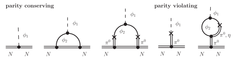
Figure 11: The leading order and one loop induced $\phi_{1}$-couplings to nucleons grouped into parity conserving coupling $g_{1NN}$ (even in $g_{A}$) and parity violating coupling $\tilde{g}_{1NN}$ in (66) (odd in $g_{A}$). The 3rd diagram is the only non-vanishing contribution to $g_{1NN}$ in BM2.

Numerically, we have for BM1, setting $m_{\phi_{2}}=1$ GeV,

$$g_{1NN}^{\rm BM1} \simeq 3.5(4.3)\times 10^{-7}\,\text{GeV}^{-1}\left(\frac{g_{dd}}{10^{-3}}\right)^{2}\,,$$ (70)

$$\tilde{g}_{1NN}^{\rm BM1} \simeq\phantom{-}4\times 10^{-6}\,\text{GeV}^{-1}\left(\frac{g_{dd}}{10^{-3}}\right)^{2}\,,$$ (71)

where the $g_{1NN}^{\rm BM1}$ central value refers to protons (neutrons), while for BM2,

$$g_{1NN}^{\rm BM2} \simeq 8\times 10^{-11}\,\text{GeV}^{-1}\left(\frac{g_{dd}}{3\times 10^{-5}}\right)^{2}\,,$$ (72)

$$\tilde{g}_{1NN}^{\rm BM2} =0\;.$$ (73)

Below we analyse the combined constraints from the previous two subsections.

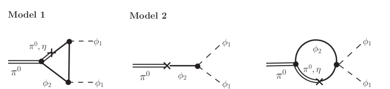
Figure 12: Diagrams for the invisible pion decay, $\pi^{0}\to\phi_{1}\phi_{1}$, in Model 1 (left) and Model 2 (middle and right). The diagram for Model 3 are analogous to Model 2 with the difference that the graph on the right needs an extra $\psi_{2}$ propagator as in Fig. 18.

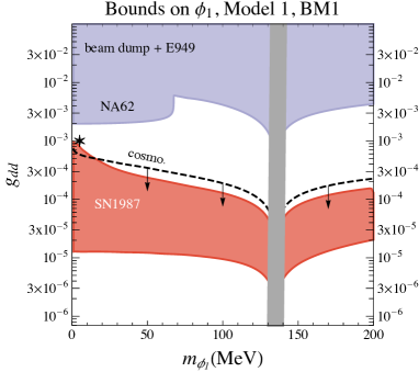
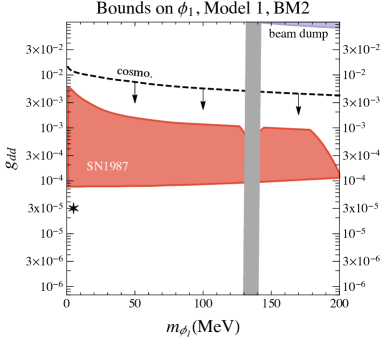
Figure 13: The constraints on the $g_{dd}$ coupling in BM1 (left) and BM2 (right) due to couplings of $\phi_{1}$ to photons and nucleons as a function of the $\phi_{1}$ mass. The purple regions are excluded by beam dump searches, E949 ($K^{+}\to\pi^{+}X$) and NA62($\pi^{0}\to{\rm inv}$), the red region by SN1987, while the dashed line shows the upper bound from cosmology in the absence of any other light states or $\phi_{1}$-couplings. The star denotes the values of $g_{dd}$ and $m_{\phi_{1}}$ in Fig. 5 (Fig. 6) for BM1 (BM2). The region around $m_{\phi_{1}}\simeq m_{\pi^{0}}$ is masked out (gray region).

3.5.5 Combined analysis of $\phi_{1}$-constraints

The most important constraint on the $\phi_{1}$-couplings comes from the neutrino burst duration observed in the supernova SN1987A. The interactions of $\phi_{1}$ with matter inside an exploding supernova are dominated by its couplings to nucleons. For $m_{\phi_{1}}=1$ MeV, used in our benchmarks, the SN1987A observations exclude $g_{1NN}^{\rm eff}\equiv(\tilde{g}_{1NN}^{2}+(3/2)g_{1NN}^{2})^{1/2}$ in the range $7\cdot 10^{-10}\,\text{GeV}^{-1}\lesssim g_{1NN}^{\rm eff}\lesssim 4\cdot 10^{-6}\,\text{GeV}^{-1}$ Lee (2018). For larger values of $g_{1NN}^{\rm eff}$ the $\phi_{1}$ gets trapped inside the proto-neutron star (PNS) and does not contribute to the cooling. This is the case for BM1, see Eqs. (70), (71). For smaller values of $g_{1NN}^{\rm eff}$ the emission of $\phi_{1}$ is suppressed sufficiently that it again does not contribute appreciably to the cooling of PNS. BM2 falls in this regime, see Eqs. (72), (73).

The photon couplings of $\phi_{1}$ are less relevant for SN1987A since the Primakoff emission of $\phi_{1}$ is always subdominant relative to the emission of $\phi_{1}$ in nucleon-nucleon scattering. This is best illustrated by the fact that SN1987A would exclude the range $10^{-8}\text{GeV}^{-1}\lesssim g_{1\gamma\gamma},h_{1\gamma\gamma}\lesssim 10^{-5}\text{GeV}^{-1}$, if $\phi_{1}$ were to coupled to photons only. The induced couplings of $\phi_{1}$ to photons are at the lower edge of this range for BM1 and well below for BM2, cf. Eqs. (58) and (59) respectively. This should be contrasted with nucleon couplings which for BM1 traps $\phi_{1}$ inside the PNS as it is above and not below the exclusion window.

The constraints from the SN1987A neutrino burst duration are shown for a range of ${\phi_{1}}$ masses for benchmarks BM1 and BM2 in Fig. 13 (left) and (right) as red regions, respectively. According to the analysis of Ref. Lee (2018), the bounds are relevant all the way up to $m_{\phi_{1}}\lesssim 300$ MeV, though we truncate the plots at 200 MeV. These bounds may however depend on the details of the SN1987A explosion, and may even be absent if this was due to a collapse-induced thermonuclear explosion Bar et al. (2019).

In addition, Fig. 13 shows with purple shading the constraints from beam dump experiments (we use the combined limit as quoted in Lee (2018)), and from the invisible pion decay by NA62 Volpe . The $\phi_{1}-\pi^{0}$ mixing angle $s_{\theta}$ needs to be smaller than about $2\times 10^{-5}$ in order to satisfy the $K^{+}\to\pi^{+}X$ constraints from E949 Adler et al. (2008) and NA62 Volpe . This imposes a constraint on $g_{dd}$ that is comparable but slightly less stringent than the beam dump limit. The upper bound from cosmology, i.e., the impact of $\phi_{1}$ decays on big bang nucleosynthesis and distortions of cosmic microwave background, are shown with a dashed line Cadamuro and Redondo (2012). This bound is very sensitive to the details of the model. For instance, if the $\phi_{1}$ decays predominantly to neutrinos these bounds would be drastically modified and thus potentially irrelevant.

4 Model 2 - scalar model leading to the three-body kaon decays

Model 2 has the same field content as Model 1, except that we impose a $Z_{2}$ symmetry under which the scalar $\phi_{1}$ is odd, $\phi_{1}\to-\phi_{1}$. The relevant terms in the Lagrangian are

$${\cal L}\supset g_{qq^{\prime}}^{(2)}(\bar{q}_{L}q_{R}^{\prime})\phi_{2}+\rm{h.c.}+\lambda_{4}\phi_{2}^{2}\phi_{1}^{2}+\lambda^{\prime}m_{S}\phi_{2}\phi_{1}^{2}+\lambda^{\prime\prime}m_{S}\phi_{2}^{3}+\cdots.$$ (74)

Note that the coupling $(\bar{q}_{L}q_{R}^{\prime})\phi_{1}$ is forbidden by the $Z_{2}$-parity. Because of the $Z_{2}$ parity the $\phi_{1}$ always appears in pairs in the final state and we thus focus on the $K\to\pi\phi_{1}\phi_{1}$ transitions with leading diagrams shown in Fig. 14.

The 1st diagram in Fig. 14, proportional to the trilinear coupling $\lambda^{\prime}$, gives the same contribution to both $K^{+}\to\pi^{+}\phi_{1}\phi_{1}$ and $K^{0}\to\pi^{0}\phi_{1}\phi_{1}$ transitions in accordance with isospin. Since we are interested in violations of the GN bound, we impose the hierarchy

$$\lambda^{\prime},\lambda^{\prime\prime}\ll\lambda_{4}\;,$$ (75)

and assume $m_{S}={\mathcal{O}}(m_{K})$. For simplicity we further assume that $\phi_{1,2}$ do not have vevs, or that they are negligibly small (cf. related discussion for Model 1 in Section 3).

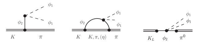
Figure 14: The diagrams inducing the $K\to\pi\phi_{1}\phi_{1}$ decays in Model 2, with the matrix elements shown in Eqs. (76) and (77). The 3rd diagram violates the GN bound.

Keeping the leading diagrams in the $\lambda^{\prime}$ and $\lambda_{4}g_{dd}^{(2)}$ expansion, i.e., the diagrams in Fig. 14, the $K_{L}\to\pi^{0}\phi_{1}\phi_{1}$ decay amplitude reads

$$\begin{split}{\cal M}(K_{L}\to\pi^{0}\phi_{1}&\phi_{1})_{\rm NP}=i\biggr{\{}4\operatorname{Im}\hat{g}_{sd}^{(2)}\operatorname{Im}g_{dd}^{(2)}\lambda_{4}\Delta_{\phi_{2}}(m_{K}^{2})\Delta_{\phi_{2}}(m_{\pi}^{2})B_{0}f_{K}f_{\pi}\\ &\qquad-2\operatorname{Im}\bar{g}_{sd}^{(2)}\lambda^{\prime}m_{S}\Delta_{\phi_{2}}(q^{2})-\frac{\operatorname{Im}\bar{g}_{sd}^{(2)}}{4\pi^{2}}\lambda_{4}{\cal F}^{(2)}_{L}(\tilde{I})B_{0}\Big{\}}B_{0}\;,\end{split}$$ (76)

with ${\cal F}^{(2)}_{L}$ given in (20), while the $K^{+}\to\pi^{+}\phi_{1}\phi_{1}$ decay amplitude is

$$\begin{split}{\cal M}(K^{+}\to\pi^{+}\phi_{1}\phi_{1})_{\rm NP}=\Big{\{}&2\bar{g}_{sd}^{(2)}\lambda^{\prime}m_{S}\Delta_{\phi_{2}}(q^{2})+\frac{\bar{g}_{sd}^{(2)}}{4\pi^{2}}\lambda_{4}B_{0}{\cal F}^{(2)}_{+}(\tilde{I})\Big{\}}B_{0}\;,\end{split}$$ (77)

with ${\cal F}^{(2)}_{+}$ defined in (21), $\tilde{I}(m_{M})=C_{0}(m_{K}^{2},q^{2},m_{\pi}^{2},m_{M}^{2},m_{\phi_{2}}^{2},m_{\phi_{2}}^{2})$, and $q^{2}=(p_{1}+p_{2})^{2}$ is the invariant mass squared of the $\phi_{1}\phi_{1}$ final state system. As for Model 1, $f^{2}\to f_{\pi}f_{K}/2$ in order to account for the main SU(3) breaking effect.

The structure of the two decay amplitudes is reminiscent of the results in Model 1 in Eqs. (18), (19). The main difference is that there is no direct coupling of $\phi_{1}$ to quarks due to the $Z_{2}$ symmetry. The $\phi_{1}\phi_{1}$ pair couples to $d\to s$ current instead through the off-shell tree level exchange of $\phi_{2}$, see the 1st diagram in Fig. 14. This leads to isospin symmetric contributions to $K^{+}\to\pi^{+}\phi_{1}\phi_{1}$ and $K_{L}\to\pi^{0}\phi_{1}\phi_{1}$, proportional to the trilinear $\lambda^{\prime}$ coupling. Hence, in the $\lambda^{\prime}\to 0$ limit, the $K^{+}\to\pi^{+}\phi_{1}\phi_{1}$ transition only receives loop contributions, and the GN bound is maximally violated. Note that $\lambda^{\prime}$ cannot be arbitrarily small, since it is generated at one loop through $\phi_{2}$ loop, $\lambda^{\prime}\sim\lambda_{4}\lambda^{\prime\prime}/(16\pi^{2})$, and at two loops with $\phi_{2}$ and $\pi^{0},\eta$ running in the loop: $\lambda^{\prime}\sim\lambda_{4}(g_{dd}^{(2)})^{3}/(16\pi^{2})^{2}$. For our benchmarks this gives a vanishingly small $\lambda^{\prime}$ and thus this contribution can be safely ignored in our analysis provided the bare value of $\lambda^{\prime},\lambda^{\prime\prime}$ are set to zero. In this limit the first isospin conserving contribution is at one loop due to the 2nd diagram in Fig. 14. The GN-violating contribution instead arises at tree level, see the 3rd diagram in Fig. 14 and the first term in (76).

The total rate of $K_{L}\to\pi^{0}\phi_{1}\phi_{1}$ adds coherently to the SM $K_{L}\to\pi^{0}\nu\bar{\nu}$ rate. The differential rate for $K_{L}\to\pi^{0}\phi_{1}\phi_{1}$ is given by

$$\frac{d\Gamma}{dE_{\pi}}=\frac{\left|{\cal M}\right|^{2}}{128\pi^{3}m_{K}}p_{\pi}\beta_{\phi_{1}}\;,$$ (78)

where $p_{\pi}=\sqrt{E_{\pi}^{2}-m_{\pi}^{2}}$ and $E_{\pi}=(m_{K}^{2}+m_{\pi}^{2}-q^{2})/(2m_{K})$ are the pion’s momentum and energy in the $K_{L}$ rest frame, while $\beta_{\phi_{1}}=(1-4m_{\phi_{1}}^{2}/q^{2})^{1/2}$.

4.1 Benchmarks for Model 2

The bounds from $K^{0}-\bar{K}^{0}$ mixing on flavor violating $\phi_{2}$-coupling $\hat{g}_{sd}^{(2)}$ are exactly the same as for Model 1, Section 3.2. To illustrate the available parameter space we therefore use the same two benchmarks for the $\phi_{2}$-couplings, Eqs. (40), (41), with results shown in Figs. 15, 16. In both cases we set $\lambda_{4}=1$ and all the other couplings, apart from the ones in Eqs. (40, 41), to zero (including $\lambda^{\prime}$). In summary, the two benchmarks for Model 2 are thus

$${\rm\bf Model~{}2,~{}BM~{}1:} \text{Eq. \eqref{eq:BM1} and~{}}m_{\phi_{1}}=100{\rm~{}MeV},\lambda_{4}=1,\,\lambda^{\prime}=\lambda^{\prime\prime}=0\;,$$ (79)

$${\rm\bf Model~{}2,~{}BM~{}2:} \text{Eq. \eqref{eq:BM2} and~{}}m_{\phi_{1}}=100{\rm~{}MeV},\lambda_{4}=1,\,\lambda^{\prime}=\lambda^{\prime\prime}=0\;,$$ (80)

while $m_{\phi_{2}}$ is kept as a free parameter. The results in Figs. 15, 16 are fairly independent of the $\phi_{1}$ mass as long as it is taken to be small, $m_{\phi_{1}}\ll m_{K}$, and thus does not modify the final phase space. The choice of benchmark value $m_{\phi_{1}}=100{\rm~{}MeV}$ is driven by the constraints of the invisible pion decays, see Section 4.2. BM1 and BM2 thus have three free parameters: $g_{dd},g_{sd}$ and $m_{\phi_{2}}$.

BM1, shown in Fig. 15, has a well restricted $\{g_{sd},m_{\phi_{2}}\}$ parameter space, since the tree level exchanges of $\phi_{2}$ contributes a new CP violating source in $K^{0}-\bar{K}^{0}$ mixing. This then restricts $g_{sd}$ to be below the hatched region in Fig. 15 (right), see also Eq. (34). However, large enhancements of $\text{Br}(K_{L}\to\pi^{0}+{\rm inv})$ over $\text{Br}(K^{+}\to\pi^{+}+{\rm inv})$ are still possible in significant parts of the parameter space. For instance, setting $g_{dd}=5\cdot 10^{-2}$, the KOTO upper bound $\text{Br}(K_{L}\to\pi^{0}\nu\bar{\nu})_{\rm exp}<3.0\times 10^{-9}$ Ahn et al. (2019) (red region in Fig. 15) are obtained for $g_{sd}\lesssim{\mathcal{O}}(10^{-9})$ and $m_{\phi_{2}}\lesssim{\mathcal{O}}(1{\rm~{}GeV})$. Fig. 15 (left) shows that in the relevant region of parameter space the deviations in $\text{Br}(K^{+}\to\pi^{+}+{\rm inv})$ from the SM prediction are negligible, while $\text{Br}(K_{L}\to\pi^{0}+{\rm inv})$ can be enhanced well above the GN bound (blue line). For illustration we vary $m_{\phi_{2}}\in[0.55,1.5]$ GeV, the same range as is shown in Fig. 15 (right), fix $g_{dd}=5\cdot 10^{-2}$ and show predictions for two choices of $g_{sd}=2\cdot 10^{-10},2\cdot 10^{-9}$ (black lines). The resulting range in $\text{Br}(K_{L}\to\pi^{0}+{\rm inv})$ is denoted with arrows. For $g_{sd}=2\cdot 10^{-9}$ the $\epsilon_{K}$ bound is reached, and the exclusion range is shown with gray dotted lines. For both choices of $g_{sd}$ the enhancements can easily be in the range of the KOTO anomaly (green band) without violating any other bounds.

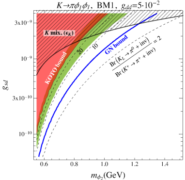
Figure 15: The parameter space for Model 2, BM1, Eq. (79). The color coding is the same as in Fig. 5. In the predictions for $\text{Br}(K^{+}\to\pi^{+}+{\rm inv})$, $\text{Br}(K_{L}\to\pi^{0}+{\rm inv})$ on the left plot (black lines) we vary $m_{\phi_{2}}\in[0.55,1.5]$ GeV for two values of $g_{sd}=2\times 10^{-10},2\times 10^{-9}$.

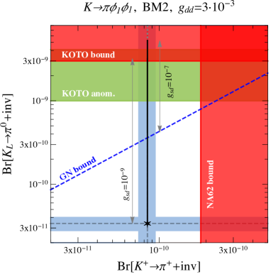
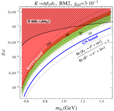
Figure 16: The preferred parameter space for Model 2, BM2. The color coding is the same as in Fig. 15. For the model predictions (black lines) in the left panel we set $g_{sd}=10^{-9},10^{-7}$ and vary $m_{\phi_{2}}\in[0.55,1.5]$ GeV.

For BM2 the allowed $\{g_{sd},m_{\phi_{2}}\}$ parameter space is much larger, since in this case $\phi_{2}$ exchanges only induce CP conserving contributions to $K^{0}-\bar{K}^{0}$ mixing. This gives the bound in (29), denoted in Fig. 16 (right) with the hatched region. Very large violations of the GN bound (blue line) are thus possible without violating $K^{0}-\bar{K}^{0}$ mixing constraints. For instance, for $g_{dd}=3\cdot 10^{-3}$ the KOTO upper bound is reached for $g_{sd}\sim$ few$\times 10^{-8}$ and $m_{\phi_{2}}\sim 1$ GeV. Fig. 16 (left) shows predictions for $\text{Br}(K^{+}\to\pi^{+}+{\rm inv})$, $\text{Br}(K_{L}\to\pi^{0}+{\rm inv})$, for two choices of $g_{sd}=10^{-9},10^{-7}$ (black lines, gray dotted line excluded by $K^{0}-\bar{K}^{0}$ mixing) when varying $m_{\phi_{2}}\in[0.55,1.5]$ GeV, setting $g_{dd}=3\cdot 10^{-3}$. The deviations in $\text{Br}(K^{+}\to\pi^{+}+{\rm inv})=1.0\cdot 10^{-8}$ vanish in BM2, while over a large region of $\{g_{dd},g_{sd},m_{\phi_{2}}\}$ the KOTO upper limits on $\text{Br}(K_{L}\to\pi^{0}+{\rm inv})$ are saturated, while avoiding any other constraints.

4.2 Constraints on the $\phi_{1}$-couplings

The most stringent constraints on the couplings of $\phi_{1}$ to quarks are due to the invisible $\pi^{0}$ decay. In the $m_{\phi_{2}}\gg m_{\pi}$ limit, the $\pi^{0}\to\phi_{1}\phi_{1}$ decay amplitude is given by,

$${\cal M}(\pi^{0}\to\phi_{1}\phi_{1}) =\frac{B_{0}f}{m_{\phi_{2}}^{2}}\biggr{[}2\lambda^{\prime}m_{S}\operatorname{Im}g_{dd}^{(2)}+\frac{\lambda_{4}B_{0}}{6\pi^{2}}\operatorname{Re}g_{dd}^{(2)}\left(2\operatorname{Im}g_{dd}^{(2)}-\operatorname{Im}g_{ss}^{(2)}\right)\biggr{]}\,,$$ (81)

where the first term in the parenthesis originates from the tree level exchange of the $\phi_{2}$, Fig. 12 (middle), the second from the one loop contribution shown in Fig. 12 (right).

Using Eq. (43) for the $\pi^{0}\to\phi_{1}\phi_{1}$ partial decay width, the corresponding branching ratio in the $m_{\phi_{1}}\ll m_{\pi}\ll m_{\phi_{2}}$ limit are, setting $g_{ss}^{(2)}=0$,

$$\text{Br}(\pi^{0}\to\phi_{1}\phi_{1})=\left\{\begin{array}[]{ll}3.8\times 10^{-3}\,\lambda_{4}^{2}\left(\frac{\operatorname{Re}g_{dd}^{(2)}}{3\times 10^{-2}}\right)^{2}\left(\frac{\operatorname{Im}g_{dd}^{(2)}}{3\times 10^{-2}}\right)^{2}\left(\frac{\text{GeV}}{m_{\phi_{2}}}\right)^{4},&{\rm~{}for~{}}\lambda^{\prime}=0\;,\\ 2.1\times 10^{-7}\left(\frac{\lambda^{\prime}m_{S}}{10^{-5}\,\text{GeV}}\right)^{2}\left(\frac{\operatorname{Im}g_{dd}^{(2)}}{3\times 10^{-2}}\right)^{2}\left(\frac{\text{GeV}}{m_{\phi_{2}}}\right)^{4},&{\rm~{}for~{}}\lambda_{4}=0\;.\end{array}\right.$$ (82)

These should be compared with the experimental bound $\text{Br}(\pi^{0}\to\phi_{1}\phi_{1})<4.4\times 10^{-9}$ Volpe . For $\lambda_{4}\sim{\mathcal{O}}(1)$, which is required for large violations of the GN bound, this excludes $\phi_{1}$ masses $m_{\phi_{1}}\lesssim m_{\pi}/2$ for BM1. In BM2 the $\pi^{0}\to\phi_{1}\phi_{1}$ is forbidden due to parity, so that $\phi_{1}$ can be light, as long as the parity breaking term $\lambda^{\prime}m_{S}$ is sufficiently small.

The beam dump and SN constraints in BM1 and BM2 are very similar to the ones shown in Fig. 13 for Model 1, but with rough identification $g_{dd}\big{|}_{\rm Model~{}1}\to 1/(4\pi)\times g_{dd}\big{|}_{\rm Model~{}2}$ and $m_{\phi_{1}}\big{|}_{\rm Model~{}1}\to 2m_{\phi_{1}}\big{|}_{\rm Model~{}2}$, since the transitions now involve two $\phi_{1}$ particles in the final state. In particular, for the choices of parameters in Figs. 15 and 16 the collider and SN constraints are presumably satisfied.

4.3 $\phi_{1}$ as a dark matter candidate

Since $\phi_{1}$ is odd under the $Z_{2}$-parity, it is absolutely stable and could be a dark matter (DM) candidate. If $m_{\phi_{1}}>m_{\pi^{0}}$ the $\phi_{1}\phi_{1}\to\pi^{0}\pi^{0}$ annihilation channel is open. Below we shall see that the annihilation cross section is large enough, in part of the parameter space, such that the correct DM relic abundance is obtained. Note however, that this restricts $\phi_{1}$ to a rather narrow mass range, $m_{\pi^{0}}\leq m_{\phi_{1}}\leq(m_{K_{L}}-m_{\pi^{0}})/2$, or numerically, $135~{}{\rm MeV}\lesssim m_{\phi_{1}}\lesssim 181$ MeV.

The annihilation cross section for $\phi_{1}\phi_{1}\to\pi^{0}\pi^{0}$ process is dominated by the $\lambda_{4}$ vertex and $\phi_{2}-\pi^{0}$-conversion, while the $\phi_{2}$ $s$-channel resonance contribution is subleading, since $\lambda^{\prime}\ll\lambda_{4}$, cf. (75) and Fig. 17. Assuming a non-relativistic $\phi_{1}$, as is the case at the time of freeze-out, the leading thermally averaged cross section is given by

$$\langle\sigma v\rangle=\frac{1}{16\pi}\lambda_{4}^{2}\big{(}\operatorname{Im}g_{dd}^{(2)}\big{)}^{4}\biggr{(}\frac{B_{0}f_{\pi}}{m_{\phi_{2}}^{2}}\biggr{)}^{4}\frac{p_{\pi}}{m_{\phi_{1}}^{3}}\;,$$ (83)

where in this approximation $p_{\pi}=(m_{\psi_{1}}^{2}-m_{\pi}^{2})^{1/2}$. Taking $m_{\phi_{1}}=160$ MeV as a representative value gives

$$\langle\sigma v\rangle\simeq 3\cdot 10^{-26}\frac{{\rm cm}^{3}}{{\rm s}}\times\lambda_{4}^{2}\,\biggr{(}\frac{\operatorname{Im}{g_{dd}^{(2)}}}{2.56\times 10^{-2}}\biggr{)}^{4}\,\biggr{(}\frac{1{\rm~{}GeV}}{m_{\phi_{2}}}\biggr{)}^{4}\;,$$ (84)

which is of the right size to get the correct DM relic abundance ($3\cdot 10^{-26}{\rm cm}^{3}/{\rm s}\approx 1{\rm\,pb}$).

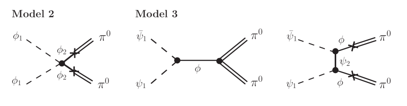
Figure 17: Graph dominating the annihilation cross section of $\phi_{1}\phi_{1}\to\pi^{0}\pi^{0}$ and $\psi_{1}\bar{\psi}_{1}\to\pi^{0}\pi^{0}$ in Model 2 and Model 3 respectively.

For $m_{\phi_{1}}<m_{\pi^{0}}$ the $\phi_{1}\phi_{1}\to\pi^{0}\pi^{0}$ annihilation cross section is kinematically forbidden. In that case the dominant annihilation channel becomes $\phi_{1}\phi_{1}\to\gamma\gamma$. The resulting annihilation cross section is so small, that if this were the only annihilation channel, the $\phi_{1}$ would overclose the universe Bertone et al. (2005). This means that $\phi_{1}$ should also couple to other light states. For instance, $\phi_{1}$ could annihilate into light SM particles, e.g. $\phi_{1}\phi_{1}\to e^{+}e^{-}$ or $\phi_{1}\phi_{1}\to\nu\bar{\nu}$. Alternatively it could annihilate away to other light dark sector particles or dark photons $\phi_{1}\phi_{1}\to\gamma_{D}\gamma_{D}$ (if $\phi_{1}$ was gauged under a dark $U(1)$). Since none of these couplings are related to $K\to\pi\phi_{1}\phi_{1}$ decays we do not explore the related phenomenology any further, beyond stating the obvious – that $\phi_{1}$ could well be a thermal relic for appropriate values of these additional couplings.

5 Model 3 - light dark sector fermions

In this model we introduce a real scalar, $\phi$, of mass $m_{\phi}$, and two Dirac fermions, $\psi_{1},\psi_{2}$, with masses $m_{\psi_{1},\psi_{2}}$, where the couplings relevant for the $K\to\pi$+inv decay are

$${\cal L}\supset g^{(\phi)}_{qq^{\prime}}(\bar{q}_{L}q_{R}^{\prime})\phi+y_{ij}\phi\bar{\psi}_{L,i}\psi_{R,j}+{\rm h.c.}\;.$$ (85)

The fermion $\psi_{2}$ is massive enough such that the decays of $K\to\pi\psi_{2}\bar{\psi}_{2}$ and $K\to\pi\psi_{1}\bar{\psi}_{2}$ are kinematically forbidden. In contrast and crucially, the decay $K\to\pi\psi_{1}\bar{\psi}_{1}$ is assumed to be kinematically allowed. The couplings of $\phi$ to the quarks are assumed to have a hierarchical flavor structure

$$g^{(\phi)}_{sd,ds}\ll g^{(\phi)}_{dd,ss}\;,$$ (86)

reflecting the suppression of flavor changing neutral currents of the SM, whereas the Yukawa couplings of $\phi$ to $\psi_{1,2}$ are assumed to favor off-diagonal transitions,

$$y_{11,22}\ll y_{12,21}\;.$$ (87)

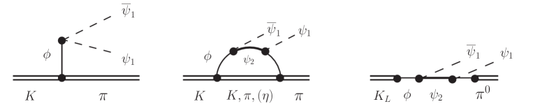
Figure 18: The $K\to\pi\psi_{1}\bar{\psi}_{1}$ in the fermion Model 3 with contribution evaluated in Eqs. (76) and (92) respectively. The third diagram only contributes to $K_{L}\to\pi^{0}\psi_{1}\bar{\psi}_{1}$, as the notation suggests, and is therefore responsible for potential violation of the GN bound in Model 3.

While we do not attempt to build a full flavor model we remark in passing that such flavor structures can easily be realised within Froggatt-Nielsen (FN) type models Froggatt and Nielsen (1979). Choosing for instance the $U(1)_{\rm FN}$ charges to be $[\psi_{L,2}]=[\psi_{R,2}]=0$, $[\psi_{L,1}]=-[\psi_{R,1}]=[\phi]=1$ and with $\epsilon=\langle\phi_{\rm FN}\rangle/M_{\rm FN}$ the FN spurion carrying the charge $[\epsilon]=-1$, the Yukawa and mass matrices take the form

$$y_{ij}\sim\begin{pmatrix}\epsilon^{*}&1\\ 1&\epsilon\end{pmatrix}\;,\quad{\cal M}_{\psi}\sim m_{0}\begin{pmatrix}\epsilon^{2}&\epsilon\\ \epsilon&1\end{pmatrix}\;,$$ (88)

where the “$\sim$” sign denotes equality up to ${\mathcal{O}}(1)$ factors. Similarly, if $[d_{L,R}]\gg[s_{R,L}]$, the $g^{(\phi)}_{sd,ds}$ can be arbitrarily suppressed in accordance with (86).

Keeping the leading diagrams in $y_{ij}$ and $g^{(\phi)}_{dd}$, shown in Fig 18, gives the following $K_{L}\to\pi^{0}\psi_{1}\bar{\psi}_{1}$ decay amplitude

$${\cal M}(K_{L} \to\pi^{0}\psi_{1}\bar{\psi}_{1})_{\rm NP}=$$

$$-i\biggr{\{} \operatorname{Im}\hat{g}^{(\phi)}_{sd}\operatorname{Im}{g}^{(\phi)}_{dd}\Delta_{\phi}(m_{K}^{2})\Delta_{\phi}(m_{\pi}^{2})\Big{[}m_{\psi_{2}}y_{12}y_{21}\big{(}\bar{u}P_{R}v\big{)}\,\bar{\Delta}+|y_{12}|^{2}\big{(}\bar{u}\gamma_{\mu}P_{L}v\big{)}\bar{\Delta}^{\mu}\Big{]}B_{0}f_{K}f_{\pi}\,$$

$$- \frac{\operatorname{Im}\bar{g}^{(\phi)}_{sd}}{16\pi^{2}}\Big{[}m_{\psi_{2}}y_{12}y_{21}\big{(}\bar{u}P_{R}v\big{)}\,{\cal F}_{L}^{(\phi)}(\bar{I}_{4})+|y_{12}|^{2}\big{(}\bar{u}\gamma_{\mu}P_{L}v\big{)}{\cal F}_{L}^{(\phi)}(\bar{I}^{\mu}_{4})\Big{]}B_{0}\,$$

$$+ \operatorname{Im}\bar{g}^{(\phi)}_{sd}\,y_{11}\big{(}\bar{u}P_{R}v\big{)}\Delta_{\phi}(q^{2})\biggl{\}}B_{0}+\big{\{}y_{ij},\gamma_{5}\leftrightarrow y^{*}_{ji},-\gamma_{5}\big{\}}\;,$$ (89)

where $2P_{R,L}\equiv 1\pm\gamma_{5}$, we have shortened $\bar{u}\equiv\bar{u}(\bar{p})$, $v\equiv v(p)$, while $q^{2}=(p+\bar{p})^{2}$ is the invariant four momentum of the fermion pair. The $\bar{\Delta}^{(\mu)}$ stands for combinations of fermion propagators

$$\bar{\Delta} \;=\; \Big{[}\Delta_{\psi_{2}}((p_{\pi}\!+\!\bar{p})^{2})+\{\bar{p}\leftrightarrow p\}\Big{]}\;,$$

$$\bar{\Delta}^{\mu} \;=\; \Big{[}(p_{\pi}+\bar{p})^{\mu}\Delta_{\psi_{2}}((p_{\pi}\!+\!\bar{p})^{2})-\{\bar{p}\leftrightarrow p\}\Big{]}\;,$$ (90)

where $\Delta_{X}(k^{2})$ is defined below (18), while ${\cal F}_{L}^{(\phi)}(Z)={\cal F}^{(2)}_{L}(Z)|_{g^{(2)}_{qq}\to g^{(\phi)}_{qq}}$, with the latter defined in (20). Its arguments are given in terms of loop integrals,

$$\bar{I}_{4}(m_{M}) \;=\;I_{4}(m_{M},\bar{p})+\big{\{}\bar{p}\to p\big{\}}\;,$$

$$\bar{I}^{\mu}_{4}(m_{M}) \;=\;\big{\{}I^{\mu}_{4}(m_{M},\bar{p})+(\bar{p}+p_{\pi})^{\mu}I_{4}(m_{M},\bar{p})\big{\}}-\big{\{}\bar{p}\to p\big{\}}\;,$$ (91)

where $I_{4}(m_{M},P)\equiv D_{0}(m_{\pi}^{2},(p_{\pi}\!+\!P)^{2},(p_{K}\!-\!p_{\pi}\!-\!P)^{2},(p_{K}\!-\!p_{\pi})^{2},P^{2},m_{K}^{2},m_{\phi}^{2},m_{M}^{2},m_{\psi_{2}}^{2},m_{\phi}^{2})$ (cf. Appendix B) and $I^{\mu}_{4}$ is the same integral with an additional Lorentz-vector $k^{\mu}$ in the integrand.

The decay amplitude $K^{+}\to\pi^{+}\psi_{1}\bar{\psi}_{1}$ is analogous, but without the 3rd diagram in Fig. 18. This gives

$$\begin{split}{\cal M}(K^{+}\to\pi^{+}\psi_{1}\bar{\psi}_{1})_{\rm NP}&=\\ -\biggr{\{}\frac{\bar{g}^{(\phi)}_{sd}}{16\pi^{2}}&\Big{[}m_{\psi_{2}}y_{12}y_{21}\big{(}\bar{u}P_{R}v\big{)}\,{\cal F}_{+}^{(\phi)}(\bar{I}_{4})+|y_{12}|^{2}\big{(}\bar{u}\gamma_{\mu}P_{L}v\big{)}{\cal F}_{+}^{(\phi)}(\bar{I}^{\mu}_{4})\Big{]}B_{0}\,\\[2.84544pt] &-\bar{g}^{(\phi)}_{sd}y_{11}\big{(}\bar{u}P_{R}v\big{)}\Delta_{\phi}(q^{2})\biggr{\}}B_{0}\!+\!\big{\{}y_{ij},\gamma_{5}\leftrightarrow y^{*}_{ji},-\gamma_{5}\big{\}}\;,\end{split}$$ (92)

where ${\cal F}_{+}^{(\phi)}(Z)={\cal F}^{(2)}_{+}(Z)|_{g^{(2)}_{qq}\to g^{(\phi)}_{qq}}$ with the later defined in (21). A formula for the rate, in differential form, is given in Appendix A.

5.1 Benchmarks for Model 3

The new elements of Model 3 are the Yukawa couplings between $\phi$ and $\psi_{1,2}$, as well as the absence of the light-scalar $\phi_{1}$. In order to ease comparisons with Model 1 and Model 2, we use $g^{(2)}_{qq^{\prime}}\to g^{(\phi)}_{qq^{\prime}}$ Eqs. (40), (41)

$${\rm\bf Model~{}3,~{}BM~{}1:}\quad g_{dd}^{(\phi)} \;=\; \tfrac{(1+i)}{\sqrt{2}}g_{dd}\;,\quad \bar{g}_{sd}^{(\phi)}\;=\;\hat{g}_{sd}^{(\phi)}=\tfrac{(1+i)}{\sqrt{2}}g_{sd}, \quad y_{12}=y_{21}=1\;,$$ (93)

$${\rm\bf Model~{}3,~{}BM~{}2:}\quad g_{dd}^{(\phi)} \;=\; ig_{dd}\;,\quad \bar{g}_{sd}^{(\phi)}\;=\;0\;,\quad\hat{g}_{sd}^{(\phi)}=ig_{sd}, \quad y_{12}=y_{21}=1\;,$$ (94)

while all the other couplings are set to zero. In particular, the only nonzero Yukawa couplings of $\psi_{i}$ fermions for $\phi$ are the flavor violating ones, $y_{12,21}$, while the diagonal ones are assumed to be vanishingly small, and set to $y_{11,22}=0$. The mass of the lightest fermion is set to $m_{\psi_{1}}=100$ MeV. The benchmarks are thus described by four continuous variables: the masses $m_{\phi},m_{\psi_{2}}$ and the real parameters $g_{dd},g_{sd}$.

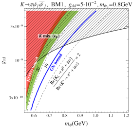
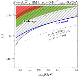
Figure 19: The parameter space for Model 3, BM1, Eq. (93). The color coding is the same as in Fig. 5. In the predictions for $\text{Br}(K^{+}\to\pi^{+}+{\rm inv})$, $\text{Br}(K_{L}\to\pi^{0}+{\rm inv})$ in the left plot (black lines) we vary $m_{\phi}\in[0.55,1.2]$ GeV for two values of $g_{sd}=10^{-10},10^{-9}$ and fix $m_{\psi_{2}}=0.8$ GeV. Right (middle) panels show the parameter space as functions of $m_{\psi_{2}}(m_{\phi})$, fixing $m_{\phi(\psi_{2})}=0.8$ GeV.

The flavor violating coupling, $\hat{g}_{sd}^{(\phi)}$, is constrained by $K^{0}-\bar{K}^{0}$ mixing. The bounds are the same as for $\phi_{2}$ in Model 1, Section 3.2, and are thus obtained from Eqs. (34), (29) through the $\hat{g}_{sd}^{(2)}\to\hat{g}_{sd}^{(\phi)}$, $m_{\phi_{2}}\to m_{\phi}$ replacements. BM1 is severely constrained by $\epsilon_{K}$ since tree level exchange of $\phi$ induces a new CP violating contribution to $K^{0}-\bar{K}^{0}$ mixing. Fig. 19 (middle) and (right) show that large enhancements of $\text{Br}(K_{L}\to\pi^{0}+{\rm inv})/\text{Br}(K^{+}\to\pi^{+}+{\rm inv})$ are possible only for small values of $m_{\phi}$ and $m_{\psi_{2}}$, comparable to the kaon mass. Still, such light NP states are not excluded experimentally and can saturate the present KOTO bound. Fig. 19 (left) shows that in this regime it is possible to have values for this ratio well above the GN bound, in the range of the anomalous KOTO events (green band).

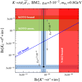
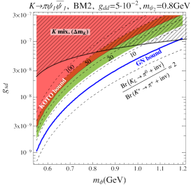
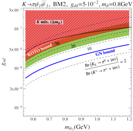
Figure 20: Same as Fig. 19 but for Model 3 BM2. In the predictions for $\text{Br}(K^{+}\to\pi^{+}+{\rm inv})$, $\text{Br}(K_{L}\to\pi^{0}+{\rm inv})$ in the left plot (black lines) we vary $m_{\phi}\in[0.55,1.2]$ GeV for two values of $g_{sd}=7\cdot 10^{-9},7\cdot 10^{-7}$ and fix $m_{\psi_{2}}=0.8$ GeV.

BM2, on the other hand, does not lead to tree level contributions to $\epsilon_{K}$. The constraints from $K^{0}-\bar{K}^{0}$ mixing are therefore relaxed compared to BM1 as they are only due to $\Delta m_{K}$. As shown in Fig. 20, it is thus possible to saturate the present KOTO upper bounds over a much larger set of parameter space, with masses of $m_{\phi}$ and $m_{\psi_{2}}$ up to $\sim 1$ GeV for $g_{dd}=5\cdot 10^{-2}$. Next, we discuss the constraints on the $\psi_{1}$-couplings.

5.2 Constraints on the $\psi_{1}$-couplings

The leading diagrams for $\pi^{0}\to\psi_{1}\bar{\psi}_{1}$, relevant to the invisible pion constraint, are analogous to the Model 2 ones shown in Fig. 12 with $\phi_{2}\to\phi$, $\phi_{1}\to\psi_{1}$ with a $\psi_{2}$ inserted in between the final state pair in the loop diagram. Assuming $m_{\phi,\psi_{2}}\gg m_{\pi,\eta}$, the corresponding matrix element reads

$${\cal M}(\pi^{0}\to\psi_{1}\bar{\psi}_{1})=\big{(}\bar{u}P_{R}v\big{)}\frac{B_{0}f}{m_{\phi}^{2}}\hat{\cal M}+\big{\{}y_{ij},\gamma_{5}\leftrightarrow y^{*}_{ji},-\gamma_{5}\big{\}}+{\cal O}(m_{\pi}^{2}/m_{\phi,\psi_{2}}^{2})\;,$$ (95)

where $\hat{\cal M}$ is a shorthand for

$$\hat{\cal M}=\operatorname{Im}g^{(\phi)}_{dd}y_{11}+\operatorname{Re}g^{(\phi)}_{dd}y_{12}y_{21}\frac{1}{12\pi^{2}}\frac{B_{0}}{m_{\psi_{2}}}\left(2\operatorname{Im}g_{dd}^{(\phi)}-\operatorname{Im}g_{ss}^{(\phi)}\right)H(x)\;,$$ (96)

where $x=m_{\phi}^{2}/m_{\psi_{2}}^{2}$, $H(x)=(1+x(\ln x-1))/(1-x)^{2}$ quoting $H(0)=1$ and $H(1)=0.5$ as representatitve values. The total rate is easily obtained from the matrix element squared given in (107) and the $1\to 2$ decay rate (43) (without the symmetry factor $1/2$)

$$\Gamma(\pi^{0}\to\psi_{1}\bar{\psi}_{1})=\frac{(B_{0}f_{\pi})^{2}}{m_{\phi}^{4}}\left(\beta_{\psi_{1}}^{2}(\operatorname{Re}\hat{\cal M})^{2}+(\operatorname{Im}\hat{\cal M})^{2}\right)\,\frac{m_{\pi}}{16\pi}\beta_{\psi_{1}}\;,$$ (97)

replacing $f\to f_{\pi}/\sqrt{2}$ and adapting $\beta_{\psi_{1}}=(1-4m_{\psi_{1}}^{2}/m_{\pi}^{2})^{1/2}$. Assuming $\operatorname{Im}g^{(\phi)}_{ss}=0$, $m_{\psi_{1}}=0$ and $H(x)\to 1$ one gets values

$$\text{Br}(\pi^{0}\to\psi_{1}\bar{\psi}_{1})=\begin{cases}2.6\cdot 10^{-9}\,\left(\frac{|y_{11}|}{5\cdot 10^{-6}}\right)^{2}\left(\frac{\operatorname{Im}g_{dd}^{(2)}}{5\cdot 10^{-2}}\right)^{2}\left(\frac{\text{GeV}}{m_{\phi}}\right)^{4}\,,&y_{12}y_{21}=0\,,\\ 3.3\cdot 10^{-9}\left(\frac{|y_{12}y_{21}|}{10^{-2}}\right)^{2}\left(\frac{\operatorname{Re}g_{dd}^{(2)}}{5\cdot 10^{-2}}\frac{\operatorname{Im}g_{dd}^{(2)}}{5\cdot 10^{-2}}\right)^{2}\left(\frac{\text{GeV}}{m_{\phi}}\right)^{4}\left(\frac{4\,\text{GeV}}{m_{\psi_{2}}}\right)^{2},&y_{11}=0\;,\end{cases}$$ (98)

which are close to the upper experimental bound $\text{Br}(\pi^{0}\to\phi_{1}\phi_{1})<4.4\times 10^{-9}$ Volpe . Clearly the tree graph is leading and imposes a constrain $|y_{11}|\lesssim{\mathcal{O}}(5\cdot 10^{-6})$ on the Yukawa couplings to the light fermion for the two benchmarks in Figs. 19 and 20. We observe that, for both BM1 and BM2 the lightest fermion is required to be heavy enough that invisible pion decay is kinematically forbidden, $m_{\psi_{1}}\gtrsim m_{\pi^{0}}/2$. Reducing somewhat the value of $|y_{12}y_{21}|\sim{\mathcal{O}}(10^{-2})$, very light $\psi_{1}$ are possible. Even in this case the KOTO bounds could be saturated (at least for the BM2 flavor structure of the couplings).

5.3 $\psi_{1}$ as a dark matter candidate

In the minimal version of Model 3, presented in this work, $\psi_{1}$ and $\psi_{2}$ are odd under the $Z_{2}$-parity. The lightest fermion, $\psi_{1}$ can thus be a DM candidate. The situation is similar to Model 2. For $\psi_{1}$ in the mass range $135~{}{\rm MeV}\lesssim m_{\psi_{1}}\lesssim 181$ MeV, $\psi_{1}\bar{\psi}_{1}\to\pi^{0}\pi^{0}$ is kinematically allowed, and can lead to the correct relic DM abundance. For lighter $\psi_{1}$ only the $\psi_{1}\bar{\psi}_{1}\to\gamma\gamma$ annihilation is allowed. However, if $\phi$ were to couple to electrons or neutrinos, the resulting annihilation cross sections can be large enough such that $\psi_{1}$ can be the DM.

For now, let us assume that $\psi_{1}\bar{\psi}_{1}\to\pi^{0}\pi^{0}$ is kinematically allowed. Then at leading order there are two relevant diagrams as shown in Fig. 17. The corresponding matrix element reads

$${\cal M}(\psi_{1}\bar{\psi}_{1}\to\pi^{0}\pi^{0}) \;=\; \left(B_{0}f\operatorname{Im}g_{dd}^{(\phi)}\Delta_{\phi}(m_{\pi}^{2})\right)^{2}\Big{[}m_{\psi_{2}}y_{12}y_{21}\tilde{\Delta}\big{(}\bar{v}P_{R}u\big{)}+|y_{12}|^{2}\tilde{\Delta}^{\mu}\big{(}\bar{v}\gamma_{\mu}P_{L}u\big{)}\Big{]}$$

$$+B_{0}\operatorname{Re}g_{dd}^{(\phi)}\Big{[}y_{11}\Delta_{\phi}(s)\bar{v}P_{R}u\Big{]}+\big{\{}y_{ij},\gamma_{5}\leftrightarrow y^{*}_{ji},-\gamma_{5}\big{\}}\;,$$ (99)

where $\bar{v}\equiv\bar{v}(p)$, $u\equiv u(\bar{p})$, $s\equiv q^{2}=(p+\bar{p})^{2}$, and by crossing symmetry from the right diagram in Fig. 18: $\tilde{\Delta}^{(\mu)}=\bar{\Delta}^{(\mu)}|_{p,\bar{p}\to-\bar{p},-p}$ in (5). The cross section is obtained from the spin-averaged squared matrix element (including a symmetry factor for identical final states)

$$\frac{d\sigma}{d\Omega}=\frac{\left|{\cal\overline{M}}\right|^{2}}{512\pi^{2}s}\frac{\beta_{\pi}}{\beta_{\psi_{1}}}\;,$$ (100)

where $\beta_{\pi,\psi_{1}}=(1-4m_{\pi,\psi_{1}}^{2}/s)^{1/2}$ are the respective velocities in the centre of mass frame. The thermally averaged cross section at leading order in the non-relativistic expansion is given by

$$\langle\sigma v\rangle=\frac{p_{\pi}}{32\pi m_{\psi_{1}}}|P|^{2}\;,$$ (101)

where in this approximation $p_{\pi}=(m_{\psi_{1}}^{2}-m_{\pi}^{2})^{1/2}$, and

$$P=i\{ B_{0}\mathrm{Re}\,g_{dd}^{(\phi)}\Delta_{\phi}(4m_{\psi_{1}}^{2})\operatorname{Im}y_{11}\,+$$

$$\left(B_{0}f_{\pi}\operatorname{Im}g_{dd}\Delta_{\phi}(m_{\pi}^{2})\right)^{2}\Delta_{\psi_{2}}(m_{\pi}^{2}\!-\!m_{\psi_{1}}^{2})m_{\psi_{2}}\operatorname{Im}y_{21}y_{12}\}\;,$$ (102)

is the pseudoscalar part in (106). It is easily obtained from (5.3) taking into account that the role of $u$ and $v$ are interchanged. All other contributions, such as $|S|^{2}$, vanish in the non-relativistic approximation. And for values of input parameters, $y_{11}=0$, $m_{\psi_{1}}=160~{}\text{MeV}$, and $m_{\phi}=1~{}\text{GeV}$ one obtains a total cross section

$$\langle\sigma v\rangle=3\times 10^{-26}\frac{{\rm cm}^{3}}{{\rm s}}\left(\frac{\operatorname{Im}g^{(\phi)}_{dd}}{7.5\times 10^{-2}}\right)^{4}\left(\frac{\operatorname{Im}y_{21}y_{12}}{1}\right)^{2}\left(\frac{1~{}\text{GeV}}{m_{\psi_{2}}}\right)^{2}\;,$$ (103)

which is of the right order of magnitude to produce the required relic abundance ($1{\rm\,pb}\approx 3\cdot 10^{-26}{\rm cm}^{3}s^{-1}$). In quoting the dependences in (103), we have neglected terms of ${\mathcal{O}}(m_{\pi,\psi_{1}}^{2}/m_{\psi_{2}}^{2})$.

6 Conclusions

We have presented three models that can lead to large deviations in $\text{Br}(K_{L}\to\pi^{0}+{\rm inv})$, while leaving $\text{Br}(K^{+}\to\pi^{0}+{\rm inv})$ virtually unchanged from the SM expectation. The three models are: Model 1 where the invisible decay is the two body transition $K_{L}\to\pi^{0}\phi_{1}$, Model 2 with $K_{L}\to\pi^{0}\phi_{1}\phi_{1}$ and Model 3 with $K_{L}\to\pi^{0}\psi_{1}\bar{\psi}_{1}$ three body transitions, can be viewed as representatives of a larger class of models. The scalar $\phi_{1}$ or fermion $\psi_{1}$ that escape the detector could be replaced by a dark gauge boson, or more complicated dark sector final states, without affecting our main conclusions.

Common to all these possibilities is that in addition to the invisible final state particles (in our case $\phi_{1}$ and $\psi_{1}$), there has to be at least one additional light mediator with a ${\mathcal{O}}(1~{}{\rm GeV})$-mass in order to have large violations of the Grossman-Nir bound. In Models 1 and 2 the mediator is another scalar, $\phi_{2}$, while in Model 3 there are two mediators, the fermion $\psi_{2}$ and scalar $\phi$. The scalar mediators mix with $K_{L}$ and $\pi^{0}$, which then leads to enhanced $\text{Br}(K_{L}\to\pi^{0}+{\rm inv})$ rates. The required mixings are small, and thus for large parts of parameter space the most stringent constraints are due to the present KOTO upper bound on $\text{Br}(K_{L}\to\pi^{0}+{\rm inv})$. If the anomalous events seen by KOTO turn out to be a true signal of new physics, then these models are natural candidates for their explanation.

In Models 2 and 3 the lightest states, $\phi_{1}$ and $\psi_{1}$, can be dark matter candidates. For the restricted mass range $m_{\pi}\leq m_{\phi_{1},\psi_{1}}\leq(m_{K}-m_{\pi})/2$ and suitable parameter ranges these particles can be the thermal relic. For lighter $\phi_{1}$ or $\psi_{1}$ new annihilation channels are required. For example the mediators could couple to either electrons or neutrinos, in addition to the couplings to quarks.

In the numerics we followed the principle of minimality and switched on the minimal set of couplings required for large violations of the GN bound. We took great care to ensure that the radiative corrections do not modify the assumed flavor structure and potentially invalidate our conclusions. In the future, it would be interesting to revisit our simplified models in more complete flavor models which fix all the couplings to quarks. An even more ambitious possible research direction could be to explore whether the light mediators could be tied to the SM flavor puzzle itself, e.g. along the lines of Ref. Smolkovič et al. (2019). We leave this and related open questions for future investigations.

Acknowledgements. We gratefully acknowledge the paradise conference in Tenerife, the 2nd Workshop on Hadronic Contributions to New Physics searches (HC2NP 2019), where this collaboration started. We are grateful to Alex Kagan, Antonin Portelli, and Diego Redigolo for useful discussions. JZ acknowledges support in part by the DOE grant de-sc0011784. JZ thanks the Higgs Centre for Theoretical Physics at The University of Edinburgh for the hospitality during the collaboration on this project. RZw is supported by an STFC Consolidated Grant, ST/P0000630/1. The work of RZi is supported by project C3b of the DFG-funded Collaborative Research Center TRR 257, “Particle Physics Phenomenology after the Higgs Discovery".

Appendix A The $K\to\pi\psi_{1}\bar{\psi}_{1}$ decay rate

For completeness we give here the explicit expression for the $K\to\pi\psi_{1}\bar{\psi}_{1}$ differential rate in Model 3. The expressions become rather involved because of the presence of the fermions in the final states. For instance, the analytic expression for the rate can only be given as a double differential rate since both variables enter the loop diagram, cf. Fig. 18, in a non-trivial way. At the end of the appendix we also comment on how this decay defies the helicity formalism used for semileptonic and flavor changing neutral currents.

The generic double differential rate in terms of Dalitz plot variables is given by Patrignani et al. (2016)

$$\frac{d^{2}}{dq^{2}dQ^{2}}\Gamma(K\to\pi\psi_{1}\bar{\psi}_{1})=\frac{1}{(2\pi)^{3}}\frac{1}{32m_{K}^{3}}|{\cal M}(K\to\pi\psi_{1}\bar{\psi}_{1})|^{2}\;,$$ (104)

where $q^{2}\equiv(p+\bar{p})^{2}$, $Q^{2}\equiv(p+p_{\pi})^{2}$ are the kinematic variables with ranges $4m_{\psi_{1}}^{2}<q^{2}<(m_{K}-m_{\pi})^{2}$ and $Q^{2}_{-}<Q^{2}<Q^{2}_{+}$, with

$$Q^{2}_{\mp}=(E_{\psi_{1}}+E_{\pi})^{2}-\left(p_{\psi_{1}}\pm p_{\pi}\right)^{2}\;,$$ (105)

$E_{\psi_{1}}=q/2$, $E_{\pi}=(m_{K}^{2}-q^{2}-m_{\pi}^{2})/2q$ and $p_{i}=(E_{i}^{2}-m_{i}^{2})^{1/2}$.

Decomposing the matrix element ${\cal M}$ in terms of fermion bilinears

$${\cal M}=S\bar{u}v+P\bar{u}\gamma_{5}v+V^{\mu}\bar{u}\gamma_{\mu}v+A^{\mu}\bar{u}\gamma_{\mu}\gamma_{5}v+T^{\mu\nu}\bar{u}\sigma_{\mu\nu}v\;,$$ (106)

the generic matrix element squared, summing over fermion polarizations, reads

$$|{\cal M}|^{2} =2q^{2}\big{\{}|P|^{2}+\beta_{\psi_{1}}^{2}|S|^{2}+\frac{2m_{\psi_{1}}}{q^{2}}((p+\bar{p})\!\cdot\!AP^{*}+(p-\bar{p})\!\cdot\!VS^{*}+\textrm{h.c.})$$ (107)

$$+A^{\mu}(m_{\mu\mu^{\prime}}-\beta_{\psi_{1}}^{2}g_{\mu\mu^{\prime}})A^{\mu^{\prime}*}+V^{\mu}(m_{\mu\mu^{\prime}}-g_{\mu\mu^{\prime}})V^{\mu^{\prime}*}$$

$$+2T^{\mu\nu}g_{\mu\mu^{\prime}}(g_{\nu\nu^{\prime}}-2m_{\nu\nu^{\prime}})T^{\mu^{\prime}\nu^{\prime}*}+\frac{4}{q^{2}}\left(iT^{\mu\nu}(m_{\psi_{1}}(\bar{p}-p)_{\mu}A^{*}_{\nu}+\bar{p}_{\mu}p_{\nu}P^{*})+\textrm{h.c.}\right)\big{\}}\;,$$

where $\sigma_{\mu\nu}=i/2[\gamma_{\mu},\gamma_{\nu}]$, $\beta_{\psi_{1}}=(1-4m_{\psi_{1}}^{2}/q^{2})^{1/2}$ and $m_{\mu\nu}\equiv 2(\bar{p}_{\mu}p_{\nu}+p_{\mu}\bar{p}_{\nu})/q^{2}$. For completeness we have included the tensor current in (106) even though it does not appear in our models.

The conversion from a form ${\cal M}=L\bar{u}P_{L}v+R\bar{u}P_{R}v+L^{\mu}\bar{u}\gamma_{\mu}P_{L}v+R^{\mu}\bar{u}\gamma_{\mu}P_{R}v$, used in (76), to the form in (106) proceeds via: $S[P]=1/2(R\pm L)$ and $V[A]^{\mu}=1/2(R\pm L)^{\mu}$. In particular for $K_{L}\to\pi^{0}\psi_{1}\bar{\psi}_{1}$

$$S[P]_{L} \;=\;-iB_{0}\left(B_{0}m_{\psi_{2}}\operatorname{Re}[i\operatorname{Im}](y_{12}y_{21})X_{L}+\operatorname{Re}[i\operatorname{Im}]y_{11}\operatorname{Im}\bar{g}^{(\phi)}_{sd}\Delta_{\phi}(q^{2})\right)\;,$$ (108)

$$V[A]_{L}^{\mu} \;=\;-iB_{0}^{2}/2\left(|y_{21}|^{2}\pm|y_{12}|^{2}\right)X_{L}^{\mu}\;,$$ (109)

with $X_{L}\equiv\operatorname{Im}\hat{g}_{sd}\bar{\Delta}f_{K}f_{\pi}-\frac{\operatorname{Im}\bar{g}_{sd}}{16\pi^{2}}{\cal F}_{L}^{(\phi)}(\bar{I}_{4})$ and $X_{L}^{\mu}=X_{L}|_{\bar{I}_{4},\bar{\Delta}\to\bar{I}_{4}^{\mu},\bar{\Delta}^{\mu}}$, whereas for $K^{+}\to\pi^{+}\psi_{1}\bar{\psi}_{1}$ (92) the decomposition reads

$$S[P]_{+} \;=\;B_{0}\left(B_{0}m_{\psi_{2}}\operatorname{Re}[i\operatorname{Im}](y_{12}y_{21})X_{+}+\operatorname{Re}[i\operatorname{Im}]y_{11}\bar{g}^{(\phi)}_{sd}\Delta_{\phi}(q^{2})\right)\;,$$ (110)

$$V[A]_{+}^{\mu} \;=\;B_{0}^{2}/2\left(|y_{21}|^{2}\pm|y_{12}|^{2}\right)X_{+}^{\mu}\;,$$ (111)

with $X_{+}\equiv-\frac{\bar{g}_{sd}}{16\pi^{2}}{\cal F}_{+}^{(\phi)}(\bar{I}_{4})$ and $X_{+}^{\mu}=X_{+}|_{\bar{I}_{4}\to\bar{I}_{4}^{\mu}}$.

It seems worthwhile to point out that this decay cannot be cast in the Jacob-Wick helicity formalism, since it does not corresponds to a chain of $1\to 2$ decays. This also applies, e.g., to the generalisation of the formalism to effective theories used for $B\to K\ell^{+}\ell^{-}$ Gratrex et al. (2016). The issue is that in Model 3 the $\phi$ particle breaks factorization of the fermion part and the rest in the same way as the photon does between the lepton and the quarks, cf. Section 5.3. in Ref. Gratrex et al. (2016). On a technical level, this can easily be seen from the decomposition of the vector matrix element

$$V^{\mu}=V^{(p)}p^{\mu}+V^{(\bar{p})}\bar{p}^{\mu}+V^{(p_{\pi})}p_{\pi}^{\mu}\;,$$ (112)

which necessitates all independent momenta of the decay. In the $B\to K\ell^{+}\ell^{-}$ case, induced by the standard dimension six effective Hamiltonian and no QED or electroweak corrections, the amplitude only depends on $p_{\pi}$, $p+\bar{p}$ but not the difference $p-\bar{p}$. However, using such a decomposition in the expressions given above does allow in practice for a fast numerical evaluation of the differential rate thereby retaining one of the main advantages of the helicity amplitude formalism.

Appendix B Integral conventions

For convenience and clarity we collect here the conventions of the Passarino-Veltman functions Passarino and Veltman (1979); Hahn and Perez-Victoria (1999); Patel (2015); Hahn and Perez-Victoria (1999) used in this work. The conventions are equivalent to those of LoopTools Hahn and Perez-Victoria (1999) and FeynCalc Mertig et al. (1991); Shtabovenko et al. (2016). The loop function used are the triangle and box integrals defined by

$$C_{0}(p_{1}^{2},p_{2}^{2},(p_{1}\!+\!p_{2})^{2},m_{1}^{2},m_{2}^{2},m_{3}^{2})\equiv\int_{k}\frac{1}{(k^{2}-m_{1}^{2})((k\!+\!p_{1})^{2}-m_{2}^{2}),((k\!+\!p_{1}\!+\!p_{2})^{2}-m_{2}^{2})}\;,$$ (113)

and

$$\begin{split}&D_{0}(m_{\pi}^{2},(p_{\pi}\!+\!P)^{2},(p_{K}\!-\!p_{\pi}\!-\!P)^{2},(p_{K}\!-\!p_{\pi})^{2},P^{2},m_{K}^{2},m_{\phi}^{2},m_{M}^{2},m_{\psi_{2}}^{2},m_{\phi}^{2})\equiv\\ &\qquad\qquad\int_{k}\frac{1}{((k\!+\!p_{K})^{2}\!-\!m_{\phi}^{2})((k\!+\!p_{\pi})^{2}\!-\!m_{\phi}^{2})((k\!+\!p_{\pi}\!+\!P)^{2}\!-\!m_{\psi_{2}}^{2})(k^{2}\!-\!m_{M}^{2})}\;,\end{split}$$ (114)

respectively, with $i0$-prescription suppressed and $\int_{k}\equiv(2\pi\mu)^{4\!-\!d}/(i\pi^{2})\int d^{d}k$. The arguments of the $D_{0}$ function are those appearing in Model 3 in section 5. It seems worthwhile to mention that the two-point Passarino-Veltman function does not appear in this paper and the symbol $B_{0}$ is used for a quantity related to quark condensate as stated at the beginning of Section 3.1.

References

- Grossman and Nir (1997) Y. Grossman and Y. Nir, Phys. Lett. B398, 163 (1997), arXiv:hep-ph/9701313 [hep-ph] .
- Grossman et al. (2004) Y. Grossman, G. Isidori, and H. Murayama, Phys. Lett. B 588, 74 (2004), arXiv:hep-ph/0311353 .
- He et al. (2020) X.-G. He, X.-D. Ma, J. Tandean, and G. Valencia, (2020), arXiv:2002.05467 [hep-ph] .
- Li et al. (2020) T. Li, X.-D. Ma, and M. A. Schmidt, Phys. Rev. D101, 055019 (2020), arXiv:1912.10433 [hep-ph] .
- Buras et al. (2005) A. Buras, M. Gorbahn, U. Haisch, and U. Nierste, Phys. Rev. Lett. 95, 261805 (2005), arXiv:hep-ph/0508165 .
- Brod et al. (2011) J. Brod, M. Gorbahn, and E. Stamou, Phys. Rev. D83, 034030 (2011), arXiv:1009.0947 [hep-ph] .
- Buras et al. (2015) A. J. Buras, D. Buttazzo, J. Girrbach-Noe, and R. Knegjens, JHEP 11, 033 (2015), arXiv:1503.02693 [hep-ph] .
- (8) R. Volpe, “New Result on from the NA62 Experiment,” talk presented at Pheno2020, Pittsburgh, USA, May 2020.
- Ahn et al. (2019) J. K. Ahn et al. (KOTO), Phys. Rev. Lett. 122, 021802 (2019), arXiv:1810.09655 [hep-ex] .
- (10) S. Shinohara, “Search for the rare decay at J- PARC KOTO experiment,” talk presented at KAON2019, Perugia, Italy,September 2019.
- (11) T. Nomura, “E14/KOTO Status,” talk given at 29th J-PARC PAC meeting, J-PARC, Japan, January 2020.
- Kitahara et al. (2020) T. Kitahara, T. Okui, G. Perez, Y. Soreq, and K. Tobioka, Phys. Rev. Lett. 124, 071801 (2020), arXiv:1909.11111 [hep-ph] .
- Fabbrichesi and Gabrielli (2019) M. Fabbrichesi and E. Gabrielli, (2019), arXiv:1911.03755 [hep-ph] .
- Fuyuto et al. (2015) K. Fuyuto, W.-S. Hou, and M. Kohda, Phys. Rev. Lett. 114, 171802 (2015), arXiv:1412.4397 [hep-ph] .
- Hou (2017) G. W. S. Hou, Proceedings, (KAON 2016): Birmingham, United Kingdom, 2016, J. Phys. Conf. Ser. 800, 012024 (2017), arXiv:1611.09673 [hep-ph] .
- Egana-Ugrinovic et al. (2019) D. Egana-Ugrinovic, S. Homiller, and P. Meade, (2019), arXiv:1911.10203 [hep-ph] .
- Dev et al. (2020) P. S. B. Dev, R. N. Mohapatra, and Y. Zhang, Phys. Rev. D101, 075014 (2020), arXiv:1911.12334 [hep-ph] .
- Jho et al. (2020) Y. Jho, S. M. Lee, S. C. Park, Y. Park, and P.-Y. Tseng, (2020), arXiv:2001.06572 [hep-ph] .
- Liu et al. (2020) J. Liu, N. McGinnis, C. E. M. Wagner, and X.-P. Wang, (2020), arXiv:2001.06522 [hep-ph] .
- Cline et al. (2020) J. M. Cline, M. Puel, and T. Toma, (2020), arXiv:2001.11505 [hep-ph] .
- Liao et al. (2020) Y. Liao, H.-L. Wang, C.-Y. Yao, and J. Zhang, “An imprint of a new light particle at koto?” (2020), arXiv:2005.00753 [hep-ph] .
- Hiller and Zwicky (2014) G. Hiller and R. Zwicky, JHEP 03, 042 (2014), arXiv:1312.1923 [hep-ph] .
- Christ et al. (2016) N. H. Christ, X. Feng, A. Juttner, A. Lawson, A. Portelli, and C. T. Sachrajda, Phys. Rev. D94, 114516 (2016), arXiv:1608.07585 [hep-lat] .
- Gasser and Leutwyler (1985) J. Gasser and H. Leutwyler, Nucl. Phys. B250, 465 (1985).
- Pich (1995) A. Pich, Rept. Prog. Phys. 58, 563 (1995), arXiv:hep-ph/9502366 [hep-ph] .
- Aoki et al. (2019) S. Aoki et al. (Flavour Lattice Averaging Group), (2019), arXiv:1902.08191 [hep-lat] .
- Tanabashi et al. (2018) M. Tanabashi et al. (Particle Data Group), Phys. Rev. D 98, 030001 (2018).
- Mescia and Smith (2007) F. Mescia and C. Smith, Phys. Rev. D 76, 034017 (2007), arXiv:0705.2025 [hep-ph] .
- Adler et al. (2008) S. Adler et al. (E949, E787), Phys. Rev. D77, 052003 (2008), arXiv:0709.1000 [hep-ex] .
- Buras et al. (2010) A. J. Buras, D. Guadagnoli, and G. Isidori, Phys. Lett. B688, 309 (2010), arXiv:1002.3612 [hep-ph] .
- Brod et al. (2019) J. Brod, M. Gorbahn, and E. Stamou, (2019), arXiv:1911.06822 [hep-ph] .
- Bona et al. (2008) M. Bona et al. (UTfit), JHEP 03, 049 (2008), arXiv:0707.0636 [hep-ph] .
- (33) U. Collaboration, http://www.utfit.org/UTfit/, summer 2018 results.
- Cirigliano et al. (2012) V. Cirigliano, G. Ecker, H. Neufeld, A. Pich, and J. Portoles, Rev. Mod. Phys. 84, 399 (2012), arXiv:1107.6001 [hep-ph] .
- D’Ambrosio and Isidori (1998) G. D’Ambrosio and G. Isidori, Int. J. Mod. Phys. A 13, 1 (1998), arXiv:hep-ph/9611284 .
- Charles et al. (2005) J. Charles, A. Hocker, H. Lacker, S. Laplace, F. Le Diberder, J. Malcles, J. Ocariz, M. Pivk, and L. Roos (CKMfitter Group), Eur. Phys. J. C 41, 1 (2005), summer 2019 update, arXiv:hep-ph/0406184 .
- Abbott et al. (2020) R. Abbott et al. (RBC, UKQCD), (2020), arXiv:2004.09440 [hep-lat] .
- Aebischer et al. (2020) J. Aebischer, C. Bobeth, and A. J. Buras, (2020), arXiv:2005.05978 [hep-ph] .
- Artamonov et al. (2009) A. V. Artamonov et al. (BNL-E949), Phys. Rev. D79, 092004 (2009), arXiv:0903.0030 [hep-ex] .
- (40) G. Ruggiero, “Latest measurement of with the NA62 experiment at CERN,” talk presented at KAON2019, Perugia, Italy,September 2019.
- Artamonov et al. (2005) A. Artamonov et al. (E949), Phys. Rev. D 72, 091102 (2005), arXiv:hep-ex/0506028 .
- Altmannshofer et al. (2019) W. Altmannshofer, S. Gori, and D. J. Robinson, (2019), arXiv:1909.00005 [hep-ph] .
- Jaeckel and Spannowsky (2016) J. Jaeckel and M. Spannowsky, Phys. Lett. B753, 482 (2016), arXiv:1509.00476 [hep-ph] .
- Jenkins and Manohar (1991) E. E. Jenkins and A. V. Manohar, Phys. Lett. B255, 558 (1991).
- Bishara et al. (2017) F. Bishara, J. Brod, B. Grinstein, and J. Zupan, JHEP 11, 059 (2017), arXiv:1707.06998 [hep-ph] .
- Simma (1994) H. Simma, Z. Phys. C 61, 67 (1994), arXiv:hep-ph/9307274 .
- Lee (2018) J. S. Lee, (2018), arXiv:1808.10136 [hep-ph] .
- Bar et al. (2019) N. Bar, K. Blum, and G. D’Amico, (2019), arXiv:1907.05020 [hep-ph] .
- Cadamuro and Redondo (2012) D. Cadamuro and J. Redondo, JCAP 1202, 032 (2012), arXiv:1110.2895 [hep-ph] .
- Bertone et al. (2005) G. Bertone, D. Hooper, and J. Silk, Phys. Rept. 405, 279 (2005), arXiv:hep-ph/0404175 [hep-ph] .
- Froggatt and Nielsen (1979) C. Froggatt and H. B. Nielsen, Nucl. Phys. B 147, 277 (1979).
- Smolkovič et al. (2019) A. Smolkovič, M. Tammaro, and J. Zupan, JHEP 10, 188 (2019), arXiv:1907.10063 [hep-ph] .
- Patrignani et al. (2016) C. Patrignani et al. (Particle Data Group), Chin. Phys. C40, 100001 (2016).
- Gratrex et al. (2016) J. Gratrex, M. Hopfer, and R. Zwicky, Phys. Rev. D93, 054008 (2016), arXiv:1506.03970 [hep-ph] .
- Passarino and Veltman (1979) G. Passarino and M. J. G. Veltman, Nucl. Phys. B160, 151 (1979).
- Hahn and Perez-Victoria (1999) T. Hahn and M. Perez-Victoria, Comput. Phys. Commun. 118, 153 (1999), arXiv:hep-ph/9807565 [hep-ph] .
- Patel (2015) H. H. Patel, Comput. Phys. Commun. 197, 276 (2015), arXiv:1503.01469 [hep-ph] .
- Mertig et al. (1991) R. Mertig, M. Bohm, and A. Denner, Comput. Phys. Commun. 64, 345 (1991).
- Shtabovenko et al. (2016) V. Shtabovenko, R. Mertig, and F. Orellana, Comput. Phys. Commun. 207, 432 (2016), arXiv:1601.01167 [hep-ph] .