Optimal Scheduling of Age-centric Caching: Tractability and Computation

Abstract

The notion of age of information (AoI) has become an important performance metric in network and control systems. Information freshness, represented by AoI, naturally arises in the context of caching. We address optimal scheduling of cache updates for a time-slotted system where the contents vary in size. There is limited capacity for the cache and for making content updates. Each content is associated with a utility function that is monotonically decreasing in the AoI. For this combinatorial optimization problem, we present the following contributions. First, we provide theoretical results settling the boundary of problem tractability. In particular, by a reformulation using network flows, we prove the boundary is essentially determined by whether or not the contents are of equal size. Second, we derive an integer linear formulation for the problem, of which the optimal solution can be obtained for small-scale scenarios. Next, via a mathematical reformulation, we derive a scalable optimization algorithm using repeated column generation. In addition, the algorithm computes a bound of global optimum, that can be used to assess the performance of any scheduling solution. Performance evaluation of large-scale scenarios demonstrates the strengths of the algorithm in comparison to a greedy schedule. Finally, we extend the applicability of our work to cyclic scheduling.

1 Introduction

The research interest in age of information (AoI) has been rapidly growing in the recent years. The notion of AoI has been introduced for characterizing the freshness of information [1]. AoI is defined as the amount of time elapsed with respect to the time stamp of the information received in the most recent update. The AoI grows linearly between two successive updates. For a wide range of control and network systems, e.g., status monitoring via sensors, AoI has become an important performance metric.

The AoI aspect arises naturally in the context of caching for holding content items with dynamic updates [2]. Consider a local cache for which updates of content items take place via a network such as a backhaul link in wireless systems. Rather than obtaining content items via the backhaul network, users can download them from the cache if the content items of interest are in the cache, thus reducing network resource consumption. Due to limited backhaul network capacity, not all content items in the cache can be updated simultaneously. Hence, at a time point, the performance of caching depends on not only the content items currently in the cache, but also how old these items are; the latter can be characterized by AoI.

We address optimal scheduling of cache updates, where the utility of the cache is based on AoI. The system under consideration is time-slotted, with a given scheduling horizon. The content items are of different sizes. Updating the cache in a time slot is subject to a capacity limit, constraining which content items that can be downloaded in the same time slot. Moreover, the cache itself has a capacity. For each content item, there is a utility function that is monotonically decreasing in the AoI, and because the content items differ in popularity, the utility function is content-specific. If a content item is not in the cache, the utility value is zero. For every time slot, the optimization decision consists of the selection of the content items to be updated, subject to the network and cache capacity constraints. Thus the problem falls in the domain of combinatorial optimization. The objective is to find the schedule maximizing the total utility over the scheduling horizon.

Our work consists in the following contributions toward understanding and solving the outlined AoI-driven cache optimization problem (ACOP).

• We provide theoretical results of problem tractability. Specifically, for the special case of uniform content size, the global optimum of ACOP admits polynomial-time tractability (even if the problem remains combinatorial optimization). We establish this result via mapping the problem to a graph, and proving that the optimal schedule is a minimum-cost flow in the graph. For non-uniform content size, the problem is NP-hard due to the knapsack structure, except for two contents. Thus our results settle the boundary of problem tractability.

• We derive an integer linear programming (ILP) formulation for ACOP in its general form, enabling the use of off-the-shelf optimization solvers to approach the problem. This is particularly useful for examining the performance of sub-optimal solutions for small-scale scenarios, for which the global optimum is computed via ILP.

• We derive a mathematical reformulation, by considering sequences representing the evolution of the AoI over time for each content item. The reformulation enables a scalable solution approach. Specifically, we present a column generation algorithm that addresses the linear programming (LP) version of the reformulation, by keeping only a small subset of possible sequences and augmenting the subset based on optimality condition. To obtain integrality, we present a rounding concept based on disjunctions rather than on fractional variables, such that column generation is repeated for improvement after rounding. Performance evaluation demonstrates the strengths of the repeated column generation algorithm in comparison to a greedy schedule. Moreover, as the algorithm provides an optimality bound in addition to a problem solution, it is possible to gauge performance even if the global optimum is out of reach. Using the bound, our results show the algorithm consistently yields near-to-optimal solutions for large-scale problem instances.

• Finally, we discuss the extension of our results to cyclic scheduling, i.e., the schedule is repeated in a cyclic manner. In this case, the AoI values at the beginning of the schedule are determined by the caching updates made later in the schedule. We present adaptations, such that the tractability analysis, the ILP formulation, and the repeated column generation algorithm all remain applicable.

2 Related Work

The notion of AoI was introduced in [1]. Generalizations to multiple information sources have been studied in [3]. The aspect of queue management has been introduced in [4, 5, 6]. Early application scenarios of AoI include channel information [7] and energy harvesting [8]. In [9], the authors address optimal update policy for AoI, and provide conditions under which the so called zero-wait policy is optimal. In [10], the authors have considered AoI under a pull model, where information freshness is relevant (only) when the use interest arises. For transmission scheduling with AoI minimization, [11] considers a system model with error probability of transmission, and [12] proposes algorithms for multiple link scheduling with presence of interference. We refer to [13] for a comprehensive survey of research on AoI. Below we outline very recent developments that demonstrate a rapidly growing interest in the topic.

One line of research has consisted in sampling, scheduling and updating policies for various system models that have queuing components and AoI as the performance objective. In [14], the scenario has multiple source-destination pairs with a common queue, along with a scheduler. In [15], the authors have investigated optimal sampling strategies addressing AoI as well as error in estimating the state of a Markov source. The system model in [16] combines stochastic status updates and unreliable links; the authors make an approximation of the Whittle index and derive a solution algorithm thereby. The study in [17] considers an energy-constrained server that is able to harvest energy when no packet from the source requires service. The notion of preemption has been addressed in [18, 19] for a single flow in a multi-hop network with preemptive intermediate nodes, and multiple flows such that different flows preempt each other, respectively. The authors of [20] have proposed the use of dynamic pricing to provide AoI-dependent incentives to sampling and transmission. For network control systems (NCPs), [21] has addressed sampling and scheduling, relating estimation error to AoI, and [22] has focused on approximately optimal scheduling strategy for multi-loop NCPs, where the centralized scheduler takes a decision based on observed AoI.

Another line of research arises from the introduction of AoI to various applications and networking context. By including energy constraints, [23] extends [12] for optimal link activation for AoI minimization in wireless networks with interference. The study in [24] is similar to [12] and [23] in terms of the scheduling aspect and the presence of interference, however the system model considers AoI for all node pairs of the network, and the emphasis is on performance bounds. The work in [25] considers a two-way data exchanging system, where the AoI is constrained by the uplink transmission capability and the downlink energy transfer capability. Application of the AoI concept in camera networks where information from multiple cameras are correlated has been presented in [26]. For remote sensor scenarios, [27] has studied AoI-optimal trajectory planning for unmanned aerial vehicles (UAVs). For distributed content storage, AoI has been applied to address the trade-off between delay and data staleness [28]. In [29], the authors have studied AoI with respect to orthogonal multiple access (OMA) and non-orthogonal multiple access (NOMA), and revealed that NOMA, even though allowing for better spectral efficiency, is not always better than OMA in terms of average AoI.

AoI has also appeared as the performance metric in using machine learning as a tool in communication systems. In [30], online adaptive learning has been used for addressing error probability in the context of AoI minimization. In [31], learning is used for optimal data sampling to minimize AoI.

For AoI-aware caching, research results are available in [2, 32]. The general problem setup, i.e., what to optimize and when to update with an objective function defined by AoI, reminds the system model we consider. However, our work has significant differences to [2] and [32]. First, it is (implicitly) assumed in [2] and [32] that the items are of uniform size. We do not have this restriction and hence in our problem, which items can be updated at a time are determined by the sizes as well as the capacity limits. Second, the works in [2] and [32] derive updating policy with respect to expected AoI, whereas our problem falls into the domain of combinatorial optimization and we use methods thereof to solve the problem. Moreover, the problems in [2, 32] are approached by either assuming given inter-update intervals of each item or the total number of updates of each item. In our work, these entities remain optimization variables throughout the optimization process.

3 Preliminaries

3.1 System Model

Consider a cache of capacity $C$. The content items for caching form a set ${\mathcal{I}}=\{1,\dots,I\}$. Item $i\in{\mathcal{I}}$ is of size $s_{i}$. Time is slotted, and the time horizon consists of a set of time slots ${\mathcal{T}}=\{1,\dots T\}$. In each time slot, the cache can be updated via a backhaul communication link whose capacity is denoted by $L$.

The AoI of an item in the cache is the time difference between the current slot and the time slot in which the item was most recently updated. Each time the item is updated, the AoI is zero, i.e., maximum information freshness. The AoI then increases by one for each time slot, until the item gets updated again. The value of having item $i$ cached is characterized by a utility function $f_{i}(\cdot)$ that is monotonically decreasing in its AoI. If the item is not in the cache, its utility is zero. The utility function is item-specific to reflect, for example, the difference in the popularity of the content items.

The AoI-driven cache optimization problem, or ACOP in short, is to determine which content items to store and update in each time slot, such that the total utility of the cache over the time horizon $1\dots T$ is maximized, subject to the capacity limits of the cache and the backhaul. Later in Section 8, we will consider the case of optimizing a cyclic schedule of cache updates.

Notation: In addition to regular mathematical style of entities, we adopt the following notation style in the paper. Sets are denoted using calligraphic style. Moreover, boldface is used to denote the vector form of the entity in question.

Remark 1.

Our system model is not necessarily restricted to caching scenarios. For example, consider a system monitoring a number of remote sites, for which the information generated differ in size. The amount of information that can be sent to the monitoring center is constrained by the network bandwidth, and the task is optimal scheduling of updates to maximize utility as a function of AoI. This setup corresponds to ACOP with redundant cache capacity. $\square$

3.2 Greedy Solution

For a combinatorial problem, a simple and greedy strategy typically serves as a reference solution. For ACOP, a greedy solution is to maximize the total utility of each time slot by simply considering the utilities of the individual items if they are added to the cache or become updated in the cache. This solution for a generic time slot is given in Algorithm 1.

Input: ${\mathcal{I}}$, $s_{i},i\in{\mathcal{I}}$, current cache ${\mathcal{H}}$, current AoI $a_{i},i\in{\mathcal{I}}$
Output: ${\mathcal{H}}$

Algorithm 1 Greedy solution for a generic time slot

1:  ${\mathcal{I}}^{\prime}\leftarrow{\mathcal{I}}$; $L^{\prime}\leftarrow L$; $r\leftarrow C-\sum_{i\in{\mathcal{H}}}s_{i}$; ${\mathcal{H}}^{\prime}\leftarrow\emptyset$

2:  while ${\mathcal{I}}^{\prime}\not=\emptyset$ and $L^{\prime}>0$ do

3:     $i^{*}\leftarrow\text{argmax}_{i\in{\mathcal{I}}^{\prime}}f_{i}(0)$

4:     ${\mathcal{I}}^{\prime}\leftarrow{\mathcal{I}}^{\prime}\setminus\{i^{*}\}$

5:     if $i^{*}\in{\mathcal{H}}$ then

6:        Update cache item $i^{*}\in{\mathcal{H}}$

7:        ${\mathcal{H}}^{\prime}\leftarrow{\mathcal{H}}^{\prime}\cup{i^{*}}$

8:     else

9:        if $r+\sum_{i\in{\mathcal{H}}\setminus{\mathcal{H}}^{\prime}}s_{i}\geq s_{i^{*}}$ and $s_{i^{*}}\leq L^{\prime}$ then

10:           while $r<s_{i^{*}}$ do

11:              $i^{\prime}\leftarrow\text{argmin}_{i\in{\mathcal{H}}}f_{i}(a_{i})$

12:              ${\mathcal{H}}\leftarrow{\mathcal{H}}\setminus{i^{\prime}}$

13:              $r\leftarrow r+s_{i^{\prime}}$

14:           ${\mathcal{H}}\leftarrow{\mathcal{H}}\cup\{i^{*}\}$

15:           $r\leftarrow r-s_{i^{*}}$

16:           $L^{\prime}\leftarrow L^{\prime}-s_{i^{*}}$

In the algorithm, ${\mathcal{I}}^{\prime}$ is the candidate set of items for caching, $r$ is the residual cache capacity, and ${\mathcal{H}}^{\prime}$ is used to keep track of those items that are currently in the cache and selected for update. The item $i^{*}$ maximizing the utility, if added or updated, is considered and then removed from ${\mathcal{I}}^{\prime}$. If $i^{*}$ is in the cache, it gets updated and recorded in ${\mathcal{H}}^{\prime}$. Otherwise, if the remaining downloading capacity admits and there will be sufficient residual capacity by removing cached items except those in ${\mathcal{H}}^{\prime}$, the algorithm removes items in ascending order of their utility values with respect to the current AoI, followed by adding item $i^{*}$. The process ends when the candidate set ${\mathcal{I}}^{\prime}$ becomes empty.

4 Problem Complexity Analysis

ACOP apparently is in the domain of combinatorial optimization. Thus it is important to gain understanding of problem complexity, as many combinatorial problems are NP-hard (e.g., the traveling salesman problem) whereas others are tractable in terms of computing global optimum in polynomial time (e.g., matching in graphs). In this section, we present proofs to establish the boundary of tractability for ACOP. Namely, for uniform item size, ACOP is tractable, otherwise it is NP-hard except for the very special case of two content items. We denote ACOP with uniform item size by ACOP${}_{\text{u}}$.

As the capacity limits of the cache and the backhaul link imply constraints of knapsack type, it is not surprising that ACOP is NP-hard in general, with a proof based on the binary knapsack problem. This result is formalized below.

Theorem 1.

ACOP is NP-hard.

Proof:

Consider a knapsack problem with $N$ items and knapsack capacity $B$. Denote the value and weight of item $i$ by $v_{i}$ and $w_{i}$, respectively. We construct an ACOP instance by setting $T=1$ (i.e., single time slot), $I=N$, $L=C=B$, and $s_{i}=w_{i},i=1,\dots,I$. The utility function is defined such that $f_{i}(0)=v_{i},i=1,\dots,I$. Downloading a content item to the cache amounts to selecting the corresponding item in the knapsack problem. Obviously, the optimal solution maximizing the total utility of the cache leads to the optimum of the knapsack problem, and the result follows. ∎

Consider ACOP${}_{\text{u}}$ where all items are of the same size. In this case, both cache and backhaul capacities can be expressed in the number of items. Even though the problem is still combinatorial along the time dimension, we prove it is tractable, i.e., the global optimum can be computed in polynomial time. The key is to transform the problem into a minimum-cost flow problem  [33] in a specifically constructed graph. In the following, we assume that the backhaul capacity $L$ is non-redundant, i.e., $L<C$.

In optimization, a network flow problem is defined in a (directed) graph; each arc has a linear cost in the arc flow that is also subject to an upper bound and a lower bound. The latter is often zero. There are one or more source nodes and sink nodes, each generating and receiving a specified amount of flow, respectively. The total amount of flow generated at the source nodes equals that to be received by the sink nodes. The optimization task is to determine how flows go from the source nodes to the sink nodes, such that the total flow cost is minimum, subject to flow balance at the nodes as well as the upper and lower bounds of the arcs.

Figure 1: An illustration of the network flow problem corresponding to ACOP${}_{\text{u}}$.

The graph we construct for proving the tractability of ACOP${}_{\text{u}}$ is illustrated in Fig. 1. For clarity, we illustrate the construction for two items and the first two time slots. The construction of the remaining time slots follows the same pattern. There is one source node, $n_{0}$, and one sink node $n_{T}$. The source node generates $I$ flow units to be sent to the sink through the network.

The underlying rationale is as follows. There are three types of nodes. First, for each item $i$ and time slot $t$, node $\alpha_{ita}$ represents that item $i$ is in the cache in slot $t$ with age $a$. Second, nodes $n_{t},t=1,\dots,T$ act as the collection points for all items except those to be kept in the cache in time slot $t$. Third, nodes $m_{t},t=1,\dots,T-1$, are collection points for items to be added or updated in the cache.

Each arc of the graph is associated with tuple $(c,l,u)$, where $c$ is the cost per flow unit, and $l$ and $u$ are the lower and upper bounds of the arc flow, respectively. These values are shown in the figure, however not for the arcs entering the nodes $n_{t},t=1,\dots,T$ due to lack of space. For these arcs, the tuple is $(0,0,1)$. Moreover, we do not show explicitly the tuples for some arcs of time slot two for the sake of clarify; the tuple values of any such arc are the same as for the corresponding arc in the previous time slot.

Let us consider the first time slot with any integer flow solution. The $I$ flow units leaving source $n_{0}$ have to either enter $m_{0}$ or $n_{1}$. Note the maximum number of units entering $m_{0}$ has upper bound $L$, allowing at most $L$ items to be added or updated. Node $m_{0}$ has an arc of capacity one to node $\alpha_{i10}$ of item $i$, $i=1,\dots,I$. Having a flow of one unit on the arc corresponds to putting item $i$ in the cache, generating utility $f_{i}(0)$ that is equivalent to an amount of $-f_{i}(0)$ in cost minimization. There will be $L$ such items. The flow units from $n_{0}$ to $n_{1}$ correspond to the items not cached in time slot one. Note the flow lower bound of arc $(n_{0},n_{1})$ is $I-C$, meaning that at least $I-C$ flow units must enter node $n_{1}$, i.e., at least $I-C$ items are outside the cache.

For a generic time slot $t$ and item $i$, if one unit of flow enters node $\alpha_{ita}$, then the flow has two choices by graph construction. Either it goes to node $\alpha_{i(t+1)(a+1)}$, representing that item $i$ remains in the cache, with AoI $a+1$ for the next time slot and the corresponding utility, or it has to be sent to the collection node $n_{t+1}$. The latter case represents that the item is removed from the cache, and, from $n_{t+1}$, the item either enters $\alpha_{i(t+1)0}$ via node $m_{t+1}$ (i.e., item $i$ is downloaded again to the cache with AoI zero), or stays outside the cache by entering collection node $n_{2}$.

Remark 2.

In Fig. 1, some of the nodes (and hence also their adjacent arcs) are redundant. For example, no flow will enter nodes $\alpha_{122}$ and $\alpha_{123}$, because the AoI will never attain two or three in time slot two. These nodes are however kept in the figure to better reflect the general structure of graph construction. $\square$

Lemma 2.

The optimal solution to ACOP${}_{\text{u}}$ corresponds to an integer flow solution for the constructed graph with equivalent objective function value.

Proof:

Consider an optimal solution to ACOP${}_{\text{u}}$. For time slot one, $L$ items are downloaded, and the flow on arc $(n_{0},m_{0})$ is set to $L$, whereas $I-L$ units of flow are put on $(n_{0},n_{1})$. For each downloaded item $i$, we set the flow on $(m_{0},\alpha_{i10})$ to be exactly one unit, generating the (negative) cost of $-f_{i}(0)$.

Consider a generic time slot $t$. For the next time slot $t+1$, denote the number of deleted items by $I_{d}$, and the numbers of items updated and added by $I_{u}$ and $I_{e}$, respectively. Denote by ${\hat{I}}$ the number of items not in the cache in the ACOP${}_{\text{u}}$ solution for time slot $t$. Thus there are $\hat{I}$ flow units on arc $(n_{t-1},n_{t})$. If a cached item $i$ in the ACOP${}_{\text{u}}$ solution is kept in the cache in $t+1$, we set one flow unit on the arc representing this state. That is, if the AoI of $i$ is $a$, we set one flow unit on arc $(\alpha_{ita},\alpha_{i(t+1)(a+1)})$, generating a (negative) cost of $-f_{i}(a+1)$. For any item $i$ that is either to be deleted or updated for $t+1$, we set one flow unit on arc $(\alpha_{ita},n_{t})$. Thus there are $I_{d}+I_{u}$ flow units in total arriving $n_{t}$ via these arcs, and the total amount of incoming flow to $n_{t}$ equals $I_{d}+I_{u}+{\hat{I}}$.

We set $L$ flow units on arc $(n_{t},m_{t})$. Next, observe that $L=I_{e}+I_{u}$, because at optimum the backhaul capacity is always fully utilized. From $m_{t}$, for any item $i$ that is either updated or added to the cache in $t+1$, we set one unit flow on arc $(m_{t},\alpha_{i(t+1)0})$, giving the (negative) cost of $-f_{i}(0)$. By flow balance, the amount of outgoing flow on arc $(n_{t},n_{t+1})$ equals $I_{n}={\hat{I}}+I_{d}+I_{u}-L={\hat{I}}+I_{d}+I_{u}-I_{e}-I_{u}={\hat{I}}+I_{d}-I_{e}$, and we need to prove $I_{n}$ is between the flow bounds $I-C$ and $I$. If the cache is full, then clearly $I_{e}=I_{d}$, and the conclusion follows. Suppose the cache is not full (this occurs at the first few time slots if downloading capacity $L$ is much smaller than cache capacity $C$), such that the spare capacity can hold $\Delta$ items. In this case, at optimum, if $I_{d}>0$, then each deleted item will be replaced by an added item, as otherwise it is optimal not to delete. Let $\Delta^{\prime}=\Delta+I_{d}$. We have $I_{e}=\min\{L,\Delta^{\prime}\}$. Moreover, as $C-\Delta$ items are cached, the number of items outside the cache ${\hat{I}}=I-C+\Delta$. Thus $I_{n}={\hat{I}}+I_{d}-I_{e}=I-C+\Delta+I_{d}-\min\{L,\Delta^{\prime}\}$ = $I-C+\Delta^{\prime}-\min\{L,\Delta^{\prime}\}$. Note that $\Delta^{\prime}-\min\{L,\Delta^{\prime}\}\geq 0$, thus $I_{n}\geq I-C$. That $I_{n}\leq I$ follows simply from that $\Delta^{\prime}\leq C$.

In addition to the above, it is straightforward to see that the flow construction satisfies the flow balance at nodes representing the items’ possible AoI values, and adheres to the bounds of their adjacent arcs. At the last stage, for all cached items in slot $T$, we set one unit of flow from the node representing the AoI to $n_{T}$. These flow units, together with those on arc $(n_{T-1},n_{T})$ that represent the number of items outside the cache, arrive the destination node $n_{T}$ with a total flow of $I$. Hence the lemma. ∎

Lemma 3.

The optimal integer flow solution in the constructed graph corresponds to a solution of ACOP${}_{\text{u}}$ with equivalent objective function value.

Proof:

For any integer flow solution, all arcs adjacent to nodes $a_{it\alpha},i=1,\dots,I,t=1,\dots,T,a=1,\dots,T-1$, have either zero or one unit of flow. Moreover, obviously an optimal flow will have $L$ flow units on arcs $(n_{t-1},m_{t-1}),t=1,\dots,T$.

Consider the flows on the outgoing arcs of node $m_{0}$. Exactly $L$ arcs have one unit of flow, and the other arcs have zero flow. For any arc $(m_{0},\alpha_{i10})$ with one flow unit, the corresponding solution of ACOP${}_{\text{u}}$ downloads and caches item $i$ for time slot one. Doing so for all time slots gives the ACOP${}_{\text{u}}$ solution in terms of the items that are added to or updated in the cache over time. Moreover, any arc $(\alpha_{ita},\alpha_{i(t+1)(a+1)})$ with a flow unit means to keep the item $i$ in the cache from $t$ to $t+1$. Thus the flow solution leads to a caching solution for ACOP${}_{\text{u}}$. Note that the solution is feasible with respect to cache capacity. This is because there are at least $I-C$ flow units on arc $(n_{t-1},n_{t})$, and by flow balance, for any time slot $t,t=1,\dots,T$, there are at most $C$ flow units in total on the incoming arcs of $\alpha_{ita},i=1,\dots,I,t=1,\dots,T,a=1,\dots,T-1$. Finally, the constructed solution clearly gives an objective function value that equals the negation of the optimal flow cost, and the lemma follows. ∎

Theorem 4.

ACOP${}_{\text{u}}$ is tractable with polynomial-time complexity.

Proof:

The maximum possible age of any item in the cache is bounded by the number of time slots $T$. Hence the size of the constructed graph is polynomial in $I$ and $T$. Moreover, the graph is clearly acyclic. For minimum-cost flow problems with integer input, there is an optimal solution in which the arc flows are integers, and there are (strong) polynomial algorithm for the problem including that with negative costs in an acyclic graph[33]. These facts, together with Lemmas 2-3, establish the theorem. ∎

Consider now ACOP with two content items. For this special case, it is trivial to see if the cache can hold one or both items. Moreover, without loss of generality, one can assume that the backhaul capacity allows for updating one item. As a result, ACOP with two content items falls in the domain of ACOP${}_{\text{u}}$, giving the corollary below.

Corollary 5.

ACOP with two items is tractable with polynomial-time complexity.

The above observation does not generalize to three or more items, because then the capacity can no longer be interpreted in the number of items. Instead, the items’ individual sizes must be explicitly accounted for.

Remark 3.

For combinatorial optimization problems, tractable problem sub-classes are often identified by proving that a greedy solution leads to optimum. For ACOP${}_{\text{u}}$, however, the greedy solution in Section 3.1 remains sub-optimal. This is due to item-specific utility function and backhaul capacity. Consider a simple example of two items. Both are of size one. The capacity values are $C=2$ and $L=1$. For item one, the utility function $f_{1}(0)=2k$ (with $k>1$) and $f_{1}(a)=0$ for $a\geq 1$. For item two, $f_{2}(a)=k$ for $a\leq t$, and $f_{2}(a)=0$ for $a\geq t+1$. The greedy solution would cache and update item one in all time slots. Thus for $T=t$, the total utility is $2kt$. The optimal solution is to cache item two in time slot one. Then, item one is added and kept updated in the next $t-1$ time slots. This gives a total utility of $kt+2k(t-1)=3kt-2k$. As a result, the greedy solution becomes highly sub-optimal for large $t$. Thus the notion of network flows is necessary for arriving at the conclusion of the tractability of ACOP${}_{\text{u}}$. $\square$

5 Integer Linear Programming Formulation

We derive an integer linear programming (ILP) formulation for ACOP. This leads to a solution approach of using an off-the-shelf optimization solver (e.g.,[34]). Even though the approach does not scale, it can be used to obtain optimum problem instances of small size, for the purpose of performance evaluation of other algorithms.

We use binary variable $x_{ita}$ that equals one if the age of item $i$ in time slot $t$ is $a$, otherwise the variable equals zero. Note that index $a$ is up to $t-1$, because the AoI in slot $t$ can never exceed $t-1$. Also, $x_{it0}=1$ means item $i$ is added to the cache or updated for time slot $t$. Binary variable $y_{it}$ is used to indicate if item $i$ is in the cache in time slot $t$ or not. The ILP formulation is given below.

$$\max_{\bm{x},\bm{y}}\limits\ \sum_{i\in{\mathcal{I}}}\sum_{t\in{\mathcal{T}}}\sum_{a=0}^{t-1}f_{i}(a)x_{ita}\qquad$$ (1a)

$$\text{s.t.}\ \ \sum_{a=0}^{t-1}x_{ita}=y_{it},i\in{\mathcal{I}},\ t\in{\mathcal{T}}$$ (1b)

$$\hskip 5.69054pt(1-y_{i(t+1)})+x_{i(t+1)0}+x_{i(t+1)(a+1)}\geq x_{ita},\$$

$$\leavevmode\nobreak\ \leavevmode\nobreak\ \leavevmode\nobreak\ \leavevmode\nobreak\ \leavevmode\nobreak\ \leavevmode\nobreak\ \leavevmode\nobreak\ \leavevmode\nobreak\ \leavevmode\nobreak\ \leavevmode\nobreak\ i\in{\mathcal{I}},t=1,\dots,T-1,a=1,\dots,t-1$$ (1c)

$$\hskip 5.69054pt\sum_{i\in{\mathcal{I}}}s_{i}y_{it}\leq C,\ t\in{\mathcal{T}}$$ (1d)

$$\hskip 5.69054pt\sum_{i\in{\mathcal{I}}}s_{i}x_{it0}\leq L,\ t\in{\mathcal{T}}$$ (1e)

$$\hskip 5.69054ptx_{ita}\in\{0,1\},i\in{\mathcal{I}},\ t\in{\mathcal{T}},a=0,\dots,t-1$$ (1f)

$$\hskip 5.69054pty_{it}\in\{0,1\},i\in{\mathcal{I}},\ t\in{\mathcal{T}}$$ (1g)

The objective function (1a) is to maximize the overall utility. By (1b), if item $i$ is cached in a time slot $t$, i.e., $y_{it}=1$, then exactly one of the binary variables representing the possible AoI values is one, otherwise these binary variables have to be zeros. Inequality (1) states that if item $i$ is cached with AoI $a$ in a time slot, then for the next time slot, either the AoI becomes $a+1$ (represented by $x_{i(t+1)(a+1)}=1$), or it gets updated (represented by $x_{i(t+1)0}=1$), or the item is no longer in the cache (represented by $y_{it}=0$). The cache and backhaul capacity limits are formulated in (1d) and (1e), respectively.

6 Repeated Column Generation Algorithm

For efficient solution of ACOP, we propose an algorithm based on repeated column generation. Column generation is an efficient method for solving large-scale linear programs with the following two structural properties [35]. First, there are exponentially many columns (i.e., variables), hence including all is not practically feasible and the method deals with only a small subset of them. Second, identifying new columns that improve the objective function value can be performed by solving an auxiliary problem, named the subproblem. This enables successive addition of new and promising columns until optimality is reached.

6.1 Problem Reformulation

Applying column generation to ACOP is based on a reformulation. In the reformulation, a column of any item is a vector representing the caching and updating decisions of the item over all time slots. We denote by ${\mathcal{L}}_{i}$ the index set of all possible such vectors for item $i$. For each column $\ell\in{\mathcal{L}}_{i}$, there is a tuple $(b_{it\ell},u_{it\ell})$ for every time slot $t$. Both elements are binary. Specifically, a column is represented by $[(b_{i1\ell},u_{i1\ell}),(b_{i2\ell},u_{i2\ell}),\dots,(b_{iT\ell},u_{iT\ell})]$ in which $b_{it\ell}$ and $u_{it\ell}$ are one if and only if the item $i$ is cached and updated, respectively, in time slot $t$. Note that there are exactly three possible outcomes of the tuple values: $(0,0)$, $(1,0)$, and $(1,1)$. As a result, the cardinality of set ${\mathcal{L}}_{i}$ is bounded by $3^{T}$.

Because a column $\ell$ fully specifies the caching and updating solution, the associated AoI values over time are known for any given column. Hence, the total utility value of column $\ell$ for item $i$, denoted by $f_{i\ell}$, can be computed.

The problem reformulation uses a binary variable $\chi_{i\ell}$ for each item $i\in{\mathcal{I}}$ and column $\ell\in{\mathcal{L}}$. This variable is one if column $\ell$ is selected for item $i$, and zero otherwise. The reformulation is given below.

$$\max_{\bm{\chi}}\limits\ \sum_{i\in{\mathcal{I}}}\sum_{\ell\in{\mathcal{L}}}f_{i\ell}\chi_{i\ell}\qquad$$ (2a)

$$\text{s.t.}\ \ \sum_{\ell\in{\mathcal{L}}}\chi_{i\ell}=1,\ i\in{\mathcal{I}}$$ (2b)

$$\hskip 5.69054pt\sum_{i\in{\mathcal{I}}}\sum_{\ell\in{\mathcal{L}}}b_{it\ell}s_{i}\chi_{i\ell}\leq C,\ t\in{\mathcal{T}}$$ (2c)

$$\hskip 5.69054pt\sum_{i\in{\mathcal{I}}}\sum_{\ell\in{\mathcal{L}}}u_{it\ell}s_{i}\chi_{i\ell}\leq L,\ t\in{\mathcal{T}}$$ (2d)

$$\hskip 5.69054pt\chi_{i\ell}\in\{0,1\},\ i\in{\mathcal{I}},\ell\in{\mathcal{L}}_{i}$$ (2e)

In (2), (2b) states that exactly one column (i.e., caching and updating solution) has to be selected for every item. The next two constraints formulate the cache and backhaul capacity, respectively. Note that both (2) and (1) are valid optimization formulations of ACOP. However they differ in structure.

6.2 Column Generation

The structure of (2) can be exploited by using column generation. To this end, we consider the linear programming counterpart of (2), where (2e) is replaced by the relaxation $0\leq\chi_{i\ell}\leq 1,i\in{\mathcal{I}},\ell\in{\mathcal{L}}$. Moreover, for each item $i$, a small subset ${\mathcal{L}}_{i}^{\prime}\subset{\mathcal{L}}_{i}$ is used and successively augmented to approach optimality. Initially, ${\mathcal{L}}_{i}^{\prime}$ can be as small as a singleton, containing only the column representing not caching the item at all. One iteration of column generation solves the following LP.

$$\max_{\bm{\chi}}\limits\ \sum_{i\in{\mathcal{I}}}\sum_{\ell\in{\mathcal{L}}_{i}}f_{i\ell}\chi_{i\ell}\qquad$$ (3a)

$$\text{s.t.}\ \ \sum_{\ell\in{\mathcal{L}}_{i}}\chi_{i\ell}=1,\ i\in{\mathcal{I}}$$ (3b)

$$\hskip 5.69054pt\sum_{i\in{\mathcal{I}}}\sum_{\ell\in{\mathcal{L}}_{i}}b_{it\ell}s_{i}\chi_{i\ell}\leq C,\ t\in{\mathcal{T}}$$ (3c)

$$\hskip 5.69054pt\sum_{i\in{\mathcal{I}}}\sum_{\ell\in{\mathcal{L}}_{i}}u_{it\ell}s_{i}\chi_{i\ell}\leq L,\ t\in{\mathcal{T}}$$ (3d)

$$\hskip 5.69054pt0\leq\chi_{i\ell}\leq 1,\ i\in{\mathcal{I}},\ell\in{\mathcal{L}}_{i}$$ (3e)

At the optimum of (3), denote by $\lambda_{i}^{*}\leavevmode\nobreak\ (i\in{\mathcal{I}})$, $\pi_{t}^{*}\leavevmode\nobreak\ (t\in{\mathcal{T}})$, and $\mu_{t}^{*}\leavevmode\nobreak\ (t\in{\mathcal{T}})$ the corresponding optimal dual variable values of (3b), (3c) and (3d), respectively. For any item $i$, the LP reduced cost of column $\ell$ equals $f_{i\ell}-\lambda_{i}^{*}-\sum_{t\in{\mathcal{T}}}b_{it\ell}s_{i}\pi_{t}^{*}-\sum_{t\in{\mathcal{T}}}u_{it\ell}s_{i}\mu_{t}^{*}$. We are interested in knowing if there exists any column with a positive reduced cost (among those in ${\mathcal{L}}_{i}\setminus{\mathcal{L}}_{i}^{\prime}$ for item $i$). If so, adding the column to (3) shall improve the objective function value. This can be accomplished by finding the column of maximum reduced cost for each item. Clearly, the resulting optimization task decomposes by item.

Recall that any column $\ell$ is characterized by a vector of tuples of binary values $[(b_{i1\ell},u_{i1\ell}),(b_{i2\ell},u_{i2\ell}),\dots,(b_{iT\ell},u_{iT\ell})]$. Finding the column of maximum reduced cost amounts to setting binary values of the tuples, such that the corresponding reduced cost is maximized. These values represent the update and caching decisions of one item, and hence we can use the variable definitions in Section 5. The subproblem for a generic item $i$ is formulated below.

$$(\text{SP}_{i})\leavevmode\nobreak\ \leavevmode\nobreak\ \leavevmode\nobreak\ \leavevmode\nobreak\ v_{i}^{*}=\max_{\bm{x},\bm{y}}\limits\ \sum_{t\in{\mathcal{T}}}\sum_{a=0}^{t-1}f_{i}(a)x_{ita}-s_{i}\sum_{t\in{\mathcal{T}}}(\pi_{t}^{*}y_{it}+\mu_{t}^{*}x_{it0})$$ (4a)

$$\text{s.t.}\ \ \sum_{a=0}^{t-1}x_{ita}=y_{it},\ t\in{\mathcal{T}}$$ (4b)

$$\hskip 5.69054pt(1-y_{i(t+1)})+x_{i(t+1)0}+x_{i(t+1)(a+1)}\geq x_{ita},\$$

$$\leavevmode\nobreak\ \leavevmode\nobreak\ \leavevmode\nobreak\ \leavevmode\nobreak\ \leavevmode\nobreak\ \leavevmode\nobreak\ \leavevmode\nobreak\ \leavevmode\nobreak\ \leavevmode\nobreak\ \leavevmode\nobreak\ t=1,\dots,T-1,a=1,\dots,t-1$$ (4c)

$$\hskip 5.69054ptx_{ita}\in\{0,1\},\ t\in{\mathcal{T}},a=0,\dots,t-1$$ (4d)

$$\hskip 5.69054pty_{it}\in\{0,1\},\ t\in{\mathcal{T}}$$ (4e)

There are clear similarities between (4) and (1), as both concern optimizing caching and updating decisions. However, they differ in several significant aspects. First, (4) deals with a single item. Second, the cache and backhaul capacities are not present in (4) because these are addressed in (2). Finally, the objective function (4a) contains the dual variables as the purpose is to maximize the reduced cost. Note that dual variable $\lambda_{i}$ is a constant for item $i$ and hence it is not explicitly included in (4a).

Figure 2: The graph for which finding the shortest path gives the optimum of (4).

Subproblem (4) is an integer linear problem. What is less obvious is that it can be transformed into a shortest path problem that is polynomial-time solvable. This is illustrated in Fig. 2, which is a modified single-item version of the network in Fig. 1. Moreover, the dual variables appear as part of the arc costs in Fig. 2.

Theorem 6.

The shortest path from node $n_{0}$ to $n_{T}$ gives the optimal solution of (4).

Proof:

By construction and the proof of Lemma 3, a flow solution corresponds to a caching solution of the item in question. Since the graph is acyclic, a flow solution is a single path. Moreover, it is easy to verify that the total path cost equals (4a) of the corresponding caching solution, and the result follows. ∎

Remark 4.

Suppose a partial decision is taken such that an item shall not be cached at a slot. This amounts to simply deleting all the arcs entering the nodes representing the age values for that slot. Similarly, the partial decision of caching the item in a slot corresponds to deleting the arc representing the opposite. To account for a partial decision of updating the item in a slot $t$, we find first the shortest path problem from the source to node $n_{t-1}$, and then include arc $(n_{t-1},\alpha_{it0})$ and find the shortest path from $\alpha_{it0}$ to the destination node. In conclusion, solving the subproblem can easily accommodate partial decisions. This observation is useful for attaining an integer solution (Section 6.3). $\square$

Input: ${\mathcal{I}}$, ${\mathcal{T}}$, $s_{i},i\in{\mathcal{I}}$, $C$, $L$, $f_{i}(\cdot),i\in{\mathcal{I}}$
Output: $\bm{\chi}^{*}$

Algorithm 2 Column generation

1:  Initialize ${\mathcal{L}}_{i},i\in{\mathcal{I}}$

2:  Stop $\leftarrow$ False

3:  while Stop = False do

4:     Solve (3) to obtain optimum $\bm{\chi}^{*}$ and dual optimum $(\bm{\lambda}^{*},\bm{\pi}^{*},\bm{\mu}^{*})$

5:     Stop $\leftarrow$ True

6:     for $i=1,\dots,I$ do

7:        Solve (4)

8:        if $v_{i}^{*}-\lambda_{i}^{*}>0$ then

9:           Stop $\leftarrow$ False

10:           Add the column corresponding to $v_{i}^{*}$ to ${\mathcal{L}}_{i}^{\prime}$

Column generation for ACOP is summarized in Algorithm 2. Applying Algorithm 2, the optimal objective function value is the LP optimum of (2) and is therefore an upper bound (UBD) of the global optimum of ACOP. This UBD is very useful to gauge performance of any suboptimal solution, because the deviation from the global optimum is bounded by that to the UBD.

6.3 Attaining Solution Integrality

The solution by Algorithm 2 may be fractional. A naive rounding algorithm would pick some fractional $\chi$-variable of some item $i$ and round it either up to one or down to zero, depending on the value. This way of rounding is rather aggressive, however, because the caching and updating decisions over all time slots become fixed, and there would be no opportunity to make any further decision for item $i$.

We consider performing rounding more gracefully. The idea is to make a rounding decision for one item and one time slot at a time. Given the optimum LP solution $\bm{\chi}^{*}$ via column generation, we define (cf. variables used in formulation (1) in Section 5) $w_{it}=\sum_{\ell\in{\mathcal{L}}_{i}^{\prime}}b_{it\ell}\chi^{*}_{i\ell}$ and $z_{it}=\sum_{\ell\in{\mathcal{L}}_{i}^{\prime}}u_{it\ell}\chi^{*}_{i\ell}$. These entities can be interpreted as the likelihood of caching and updating item $i$ in time slot $t$, respectively. Note that for item $i$, there may be multiple (and factional) $\chi^{*}$-variables contributing to the values of $w_{it}$ and $z_{it}$. The following theorem states that, to attain an integer solution for (3), it is sufficient that $w_{it}$ and $z_{it}$, $i\in{\mathcal{I}},t\in{\mathcal{T}}$, become integer.

Theorem 7.

$\bm{\chi}^{*}$ is integer if and only if $\bm{z}$ and $\bm{w}$ are integer.

Proof:

The necessity is obvious by the definition of $\bm{z}$ and $\bm{w}$. For sufficiency, assume $\bm{z}$ and $\bm{w}$ are integer. Suppose $\bm{\chi}^{*}$ is fractional, and assume more specifically $0<\chi_{i\ell}^{*}<1$. By (3b), there must exist at least another $\chi$-variable for item $i$ that has fractional value. Let ${\hat{\mathcal{L}}}_{i}$ denote the column index set of the fractional $\chi$-variables of item $i$. Because there are no identical columns in ${\mathcal{L}}_{i}^{\prime}$, there must exist some time slot $t$, for which ${\hat{\mathcal{L}}}_{i}$ can be partitioned into two sets, ${\hat{\mathcal{L}}}_{i}^{0}$ and ${\hat{\mathcal{L}}}_{i}^{1}$, such that $b_{t\ell}=0,\ell\in{\hat{\mathcal{L}}}_{i}^{0}$ and $b_{t\ell}=1,\ell\in{\hat{\mathcal{L}}}_{i}^{1}$, and none of the two sets is empty. Thus $w_{it}=\sum_{\ell\in{\mathcal{L}}_{i}^{\prime}}b_{t\ell}\chi^{*}_{i\ell}=\sum_{\ell\in{\hat{\mathcal{L}}}_{i}^{1}}b_{t\ell}\chi^{*}_{i\ell}<1$, contradicting that $w_{it}$ is integer. The same argument applies to $\bm{z}$, and the theorem follows. ∎

By the above result, rounding can be performed on $\bm{z}$ and $\bm{w}$, instead of $\bm{\chi}^{*}$. This amounts to considering disjunctions, i.e., a partition of the $\chi$-variables into two subsets rather than considering a single $\chi$-variable (cf. the proof of Theorem 7), and assembles the use of disjunctions in branch-and-bound in solving integer programs [36]. Hence we use the term disjunction-based rounding (DR) to refer to to the rounding concept.

After performing DR, column generation is applied again. This is because additional columns may be needed to reach the LP optimum given the constraint imposed by rounding. For example, setting $y_{it}=0$ means to exclude columns $\{\ell\in{\mathcal{L}}_{i}:b_{it\ell}=1\}$ and since the current ${\mathcal{L}}_{i}^{\prime}$ is a small subset of ${\mathcal{L}}_{i}$, some new column $\ell\notin{\mathcal{L}}_{i}^{\prime}$ with $b_{it\ell}=0$ may improve the objective function. This yields the repeated column generation algorithm, or RCGA in short.

Note that, after a DR operation, both (3) and the subproblem of column generation have to comply with the rounding decision. Namely, if $y_{it}=0$ by DR, then $\{\ell\in{\mathcal{L}}_{i}^{\prime}:b_{it\ell}=1\}$ are removed from (3), and arcs representing caching the item $i$ in slot time $t$ in the subproblem graph are deleted. If $y_{it}=1$, then $\{\ell\in{\mathcal{L}}_{i}^{\prime}:b_{it\ell}=0\}$ are removed from (3), and the subproblem for item $i$ becomes two (smaller) shortest path problems, then the arc representing not being in the cache is deleted. Similar updates apply for DR on $\bm{z}$. Thus the subproblem remains polynomial-time solvable.

The details of DR is presented in Algorithm 3. In the algorithm, symbol $\leftarrow$ is used to indicate assignment of value. Symbol $\leftleftarrows$ is used to indicate that an assigned value of an optimization variable is kept fixed after the assignment. Lines $1$-$2$ calculate $\bm{z}$ and $\bm{w}$. For item $i\in\mathcal{I}$ and time slot $t\in\mathcal{T}$, Line $3$ makes the decisions of fixing $x_{it0}=1$ and $y_{it}=1$, if $z_{it}=1$, and Line $4$ discards the columns that do not comply to the decisions. Line $5$ performs the opposite decision of fixing $x_{it0}=0$ and $y_{it}=0$, if $w_{it}=0$, and the non-complying columns are discarded (Line $6$). Lines 7-10 calculate the remaining spare backhaul and cache capacities, denoted by $L^{\prime}$ and $C^{\prime}$, respectively.

Lines 11 and 12 compute the number of fractional elements of $\bm{z}$ and $\bm{w}$, denoted by $\xi$ and $\eta$, respectively. If both $\xi$ and $\eta$ equal to zero, the current solution is integer by Theorem 7. Otherwise, one DR is applied for $\bm{z}$ if $\xi>0$ (Lines 14-26). If $\bm{z}$ is integer but $\eta>0$, DR is applied to a fractional element of (Lines 28-42).

More specifically, Lines 14-15 find the fractional element of $\bm{z}$ being closest to zero, and the corresponding item and time slot. These entities are denoted by $\underaccent{\bar}{z}$, $\underaccent{\bar}{i}$, and $\underaccent{\bar}{t}$, respectively. The corresponding entities in examining the fractional element of $\bm{z}$ that is closest to one (Lines 16-17) are denoted by $\bar{z}$, $\bar{i}$, and $\bar{t}$, respectively. If $\underaccent{\bar}{z}<\bar{z}$, DR fixes $x_{\underaccent{\bar}{i}\underaccent{\bar}{t}0}$ to be zero in Line 19. Furthermore, the non-complying columns are discarded from $\mathcal{L}_{\underaccent{\bar}{i}}$ in Line 20. If $\underaccent{\bar}{z}\geq\bar{z}$, the algorithm checks whether or not there is enough remaining backhaul capacity to download item $\bar{i}$. If the answer is positive, $x_{\bar{i}\bar{t}0}$ is fixed to be one in SP${}_{\bar{i}}$ by Line 22, and the non-complying columns are deleted from $\mathcal{L}_{\bar{i}}$ by Line 23. If the remaining capacity does not permit to download $\bar{i}$, $x_{\bar{i}\bar{t}0}$ is fixed to be zero by Line 25 and the non-complying columns will be discarded from $\mathcal{L}_{\bar{i}}^{\prime}$ by Line 26. DR based on $\bm{y}$ is similar to that for $\bm{z}$, and the details are presented in Lines 28-42.

As the next step, the algorithm updates the remaining spare backhaul and cache capacity limits (Lines 44-47). Thereafter, the algorithm examines if any content item has a larger size than what can be admitted by the capacity limit in any time slot. For any such item and time slot, the corresponding variable is fixed to zero, and the non-complying columns are discarded (Lines 48-55). Finally, to ensure feasibility, an auxiliary column is added for each item (Lines 56-57). If the item is cached or updated in a time slot by the decisions made by DR thus far, the corresponding parameter is set to one. The rest of elements of the column are zeros.

Algorithm 3 DR Algorithm

1:  Compute $\bm{z}=\{z_{it},i\in\mathcal{I},t\in\mathcal{T}\}$, where $z_{it}=\sum_{\ell\in\mathcal{L}_{i}}u_{it\ell}\chi^{*}_{il}$

2:  Compute $\bm{w}=\{w_{it},i\in\mathcal{I},t\in\mathcal{T}\}$, where $w_{it}=\sum_{\ell\in\mathcal{L}_{i}}b_{it\ell}\chi^{*}_{i\ell}$

3:  $x_{it0}\leftleftarrows 1$ and $y_{it}\leftleftarrows 1$ in SP_i if $z_{it}=1$, $i\in\mathcal{I},t\in\mathcal{T}$

4:  $\chi_{i\ell}\leftleftarrows 0$ in RMP if $u_{it\ell}=0$, $i\in\mathcal{I},t\in\mathcal{T},\ell\in\mathcal{L}_{i}^{\prime}$

5:  $x_{it0}\leftleftarrows 0$ and $y_{it}\leftleftarrows 0$ in SP_i if $w_{it}=0$, $i\in\mathcal{I},t\in\mathcal{T}$

6:  $\chi_{i\ell}\leftleftarrows 0$ in RMP if $b_{it\ell}=1$, $i\in\mathcal{I},t\in\mathcal{T},\ell\in\mathcal{L}_{i}^{\prime}$

7:  $\mathcal{I}^{\prime}\leftarrow\{i\in\mathcal{I}|x_{it0}\text{ is fixed to one}\}$

8:  $\mathcal{I}^{\prime\prime}\leftarrow\{i\in\mathcal{I}|y_{it}\text{ is fixed to one}\}$

9:  $C^{\prime}\leftarrow C-\sum_{i\in\mathcal{I}^{\prime}}s_{i}$

10:  $L^{\prime}\leftarrow L-\sum_{i\in\mathcal{I}^{\prime\prime}}s_{i}$

11:  $\xi\leftarrow\underset{i\in\mathcal{I},t\in\mathcal{T}\leavevmode\nobreak\ \leavevmode\nobreak\ \leavevmode\nobreak\ \leavevmode\nobreak\ \leavevmode\nobreak\ \leavevmode\nobreak\ \leavevmode\nobreak\ \leavevmode\nobreak\ \leavevmode\nobreak\ \leavevmode\nobreak\ \leavevmode\nobreak\ \leavevmode\nobreak\ \leavevmode\nobreak\ \leavevmode\nobreak\ \leavevmode\nobreak\ \leavevmode\nobreak\ \leavevmode\nobreak\ \leavevmode\nobreak\ \leavevmode\nobreak\ \leavevmode\nobreak\ \leavevmode\nobreak\ \leavevmode\nobreak\ \leavevmode\nobreak\ \leavevmode\nobreak\ \leavevmode\nobreak\ \leavevmode\nobreak\ \leavevmode\nobreak\ }{\text{cardinality}\{z_{it}|z_{it}>0\leavevmode\nobreak\ \text{and}\leavevmode\nobreak\ z_{it}<1\}}$

12:  $\eta\leftarrow\underset{i\in\mathcal{I},t\in\mathcal{T}\leavevmode\nobreak\ \leavevmode\nobreak\ \leavevmode\nobreak\ \leavevmode\nobreak\ \leavevmode\nobreak\ \leavevmode\nobreak\ \leavevmode\nobreak\ \leavevmode\nobreak\ \leavevmode\nobreak\ \leavevmode\nobreak\ \leavevmode\nobreak\ \leavevmode\nobreak\ \leavevmode\nobreak\ \leavevmode\nobreak\ \leavevmode\nobreak\ \leavevmode\nobreak\ \leavevmode\nobreak\ \leavevmode\nobreak\ \leavevmode\nobreak\ \leavevmode\nobreak\ \leavevmode\nobreak\ \leavevmode\nobreak\ \leavevmode\nobreak\ \leavevmode\nobreak\ \leavevmode\nobreak\ \leavevmode\nobreak\ \leavevmode\nobreak\ }{\text{cardinality}\{w_{it}|w_{it}>0\leavevmode\nobreak\ \text{and}\leavevmode\nobreak\ w_{it}<1\}}$

13:  if $\xi>0$ then

14:     $\underaccent{\bar}{z}\leftarrow\underset{i\in\mathcal{I},t\in\mathcal{T}\leavevmode\nobreak\ \leavevmode\nobreak\ \leavevmode\nobreak\ \leavevmode\nobreak\ \leavevmode\nobreak\ \leavevmode\nobreak\ \leavevmode\nobreak\ \leavevmode\nobreak\ \leavevmode\nobreak\ \leavevmode\nobreak\ \leavevmode\nobreak\ \leavevmode\nobreak\ \leavevmode\nobreak\ \leavevmode\nobreak\ \leavevmode\nobreak\ \leavevmode\nobreak\ \leavevmode\nobreak\ \leavevmode\nobreak\ \leavevmode\nobreak\ \leavevmode\nobreak\ \leavevmode\nobreak\ \leavevmode\nobreak\ \leavevmode\nobreak\ \leavevmode\nobreak\ \leavevmode\nobreak\ \leavevmode\nobreak\ \leavevmode\nobreak\ }{\min\{z_{it}|z_{it}>0\leavevmode\nobreak\ \text{and}\leavevmode\nobreak\ z_{it}<1\}}$

15:     $(\underaccent{\bar}{t},\underaccent{\bar}{i})\leftarrow\underset{i\in\mathcal{I},t\in\mathcal{T}\leavevmode\nobreak\ \leavevmode\nobreak\ \leavevmode\nobreak\ \leavevmode\nobreak\ \leavevmode\nobreak\ \leavevmode\nobreak\ \leavevmode\nobreak\ \leavevmode\nobreak\ \leavevmode\nobreak\ \leavevmode\nobreak\ \leavevmode\nobreak\ \leavevmode\nobreak\ \leavevmode\nobreak\ \leavevmode\nobreak\ \leavevmode\nobreak\ \leavevmode\nobreak\ \leavevmode\nobreak\ \leavevmode\nobreak\ \leavevmode\nobreak\ \leavevmode\nobreak\ \leavevmode\nobreak\ \leavevmode\nobreak\ \leavevmode\nobreak\ \leavevmode\nobreak\ \leavevmode\nobreak\ \leavevmode\nobreak\ \leavevmode\nobreak\ \leavevmode\nobreak\ \leavevmode\nobreak\ \leavevmode\nobreak\ \leavevmode\nobreak\ }{\arg\min\{z_{it}|z_{it}>0\leavevmode\nobreak\ \text{and}\leavevmode\nobreak\ z_{it}<1\}}$

16:     $\bar{z}\leftarrow\underset{i\in\mathcal{I},t\in\mathcal{T}\leavevmode\nobreak\ \leavevmode\nobreak\ \leavevmode\nobreak\ \leavevmode\nobreak\ \leavevmode\nobreak\ \leavevmode\nobreak\ \leavevmode\nobreak\ \leavevmode\nobreak\ \leavevmode\nobreak\ \leavevmode\nobreak\ \leavevmode\nobreak\ \leavevmode\nobreak\ \leavevmode\nobreak\ \leavevmode\nobreak\ \leavevmode\nobreak\ \leavevmode\nobreak\ \leavevmode\nobreak\ \leavevmode\nobreak\ \leavevmode\nobreak\ \leavevmode\nobreak\ \leavevmode\nobreak\ \leavevmode\nobreak\ \leavevmode\nobreak\ \leavevmode\nobreak\ \leavevmode\nobreak\ \leavevmode\nobreak\ \leavevmode\nobreak\ \leavevmode\nobreak\ \leavevmode\nobreak\ \leavevmode\nobreak\ \leavevmode\nobreak\ \leavevmode\nobreak\ }{\min\{1-z_{it}|z_{it}>0\leavevmode\nobreak\ \text{and}\leavevmode\nobreak\ z_{it}<1\}}$

17:     $(\bar{t},\bar{i})\leftarrow\underset{i\in\mathcal{I},t\in\mathcal{T}\leavevmode\nobreak\ \leavevmode\nobreak\ \leavevmode\nobreak\ \leavevmode\nobreak\ \leavevmode\nobreak\ \leavevmode\nobreak\ \leavevmode\nobreak\ \leavevmode\nobreak\ \leavevmode\nobreak\ \leavevmode\nobreak\ \leavevmode\nobreak\ \leavevmode\nobreak\ \leavevmode\nobreak\ \leavevmode\nobreak\ \leavevmode\nobreak\ \leavevmode\nobreak\ \leavevmode\nobreak\ \leavevmode\nobreak\ \leavevmode\nobreak\ \leavevmode\nobreak\ \leavevmode\nobreak\ \leavevmode\nobreak\ \leavevmode\nobreak\ \leavevmode\nobreak\ \leavevmode\nobreak\ \leavevmode\nobreak\ \leavevmode\nobreak\ \leavevmode\nobreak\ \leavevmode\nobreak\ \leavevmode\nobreak\ \leavevmode\nobreak\ \leavevmode\nobreak\ \leavevmode\nobreak\ \leavevmode\nobreak\ \leavevmode\nobreak\ \leavevmode\nobreak\ }{\arg\min\{1-z_{it}|z_{it}>0\leavevmode\nobreak\ \text{and}\leavevmode\nobreak\ z_{it}<1\}}$

18:     if $(\underaccent{\bar}{z}<\bar{z})$ then

19:        $x_{\underaccent{\bar}{t}\underaccent{\bar}{i}0}\leftleftarrows 0$ in SP${}_{\underaccent{\bar}{i}}$

20:        $\chi_{\underaccent{\bar}{i}\ell}\leftleftarrows 0$ if $u_{\underaccent{\bar}{i}\underaccent{\bar}{t}\ell}=1$, $\ell\in\mathcal{L}_{\underaccent{\bar}{i}}^{\prime}$

21:     else if $(s_{\bar{i}}\leq L^{\prime})$ then

22:        $x_{\bar{i}\bar{t}0}\leftleftarrows 1$ in SP${}_{\bar{i}}$

23:        $\chi_{\bar{i}\ell}\leftleftarrows 0$ if $u_{\bar{i}\bar{t}\ell}=0$, $\ell\in\mathcal{L}_{\bar{i}}^{\prime}$

24:     else

25:        $x_{\bar{i}\bar{t}0}\leftleftarrows 0$ in SP${}_{\bar{i}}$

26:        $\chi_{\bar{i}\ell}\leftleftarrows 0$ if $u_{\bar{i}\bar{t}\ell}=1$, $\ell\in\mathcal{L}_{\bar{i}}^{\prime}$

27:  else if $\eta>0$ then

28:     $y_{it}\leftleftarrows 1$ in SP_i if $w_{it}=1$, $i\in\mathcal{I},t\in\mathcal{T}$

29:     $\chi_{i\ell}\leftleftarrows 0$ in RMP if $b_{it\ell}=0$, $i\in\mathcal{I},t\in\mathcal{T},\ell\in\mathcal{L}_{i}^{\prime}$

30:     $\underaccent{\bar}{w}\leftarrow\underset{i\in\mathcal{I},t\in\mathcal{T}\leavevmode\nobreak\ \leavevmode\nobreak\ \leavevmode\nobreak\ \leavevmode\nobreak\ \leavevmode\nobreak\ \leavevmode\nobreak\ \leavevmode\nobreak\ \leavevmode\nobreak\ \leavevmode\nobreak\ \leavevmode\nobreak\ \leavevmode\nobreak\ \leavevmode\nobreak\ \leavevmode\nobreak\ \leavevmode\nobreak\ \leavevmode\nobreak\ \leavevmode\nobreak\ \leavevmode\nobreak\ \leavevmode\nobreak\ \leavevmode\nobreak\ \leavevmode\nobreak\ \leavevmode\nobreak\ \leavevmode\nobreak\ \leavevmode\nobreak\ \leavevmode\nobreak\ \leavevmode\nobreak\ \leavevmode\nobreak\ \leavevmode\nobreak\ }{\min\{w_{it}|w_{it}>0\leavevmode\nobreak\ \text{and}\leavevmode\nobreak\ w_{it}<1\}}$

31:     $(\underaccent{\bar}{t},\underaccent{\bar}{i})\leftarrow\underset{i\in\mathcal{I},t\in\mathcal{T}\leavevmode\nobreak\ \leavevmode\nobreak\ \leavevmode\nobreak\ \leavevmode\nobreak\ \leavevmode\nobreak\ \leavevmode\nobreak\ \leavevmode\nobreak\ \leavevmode\nobreak\ \leavevmode\nobreak\ \leavevmode\nobreak\ \leavevmode\nobreak\ \leavevmode\nobreak\ \leavevmode\nobreak\ \leavevmode\nobreak\ \leavevmode\nobreak\ \leavevmode\nobreak\ \leavevmode\nobreak\ \leavevmode\nobreak\ \leavevmode\nobreak\ \leavevmode\nobreak\ \leavevmode\nobreak\ \leavevmode\nobreak\ \leavevmode\nobreak\ \leavevmode\nobreak\ \leavevmode\nobreak\ \leavevmode\nobreak\ \leavevmode\nobreak\ \leavevmode\nobreak\ \leavevmode\nobreak\ \leavevmode\nobreak\ \leavevmode\nobreak\ }{\arg\min\{w_{it}|w_{it}>0\leavevmode\nobreak\ \text{and}\leavevmode\nobreak\ w_{it}<1\}}$

32:     $\bar{w}\leftarrow\underset{i\in\mathcal{I},t\in\mathcal{T}\leavevmode\nobreak\ \leavevmode\nobreak\ \leavevmode\nobreak\ \leavevmode\nobreak\ \leavevmode\nobreak\ \leavevmode\nobreak\ \leavevmode\nobreak\ \leavevmode\nobreak\ \leavevmode\nobreak\ \leavevmode\nobreak\ \leavevmode\nobreak\ \leavevmode\nobreak\ \leavevmode\nobreak\ \leavevmode\nobreak\ \leavevmode\nobreak\ \leavevmode\nobreak\ \leavevmode\nobreak\ \leavevmode\nobreak\ \leavevmode\nobreak\ \leavevmode\nobreak\ \leavevmode\nobreak\ \leavevmode\nobreak\ \leavevmode\nobreak\ \leavevmode\nobreak\ \leavevmode\nobreak\ \leavevmode\nobreak\ \leavevmode\nobreak\ \leavevmode\nobreak\ \leavevmode\nobreak\ \leavevmode\nobreak\ \leavevmode\nobreak\ \leavevmode\nobreak\ }{\min\{1-w_{it}|w_{it}>0\leavevmode\nobreak\ \text{and}\leavevmode\nobreak\ w_{it}<1\}}$

33:     $(\bar{i},\bar{t})\leftarrow\underset{i\in\mathcal{I},t\in\mathcal{T}\leavevmode\nobreak\ \leavevmode\nobreak\ \leavevmode\nobreak\ \leavevmode\nobreak\ \leavevmode\nobreak\ \leavevmode\nobreak\ \leavevmode\nobreak\ \leavevmode\nobreak\ \leavevmode\nobreak\ \leavevmode\nobreak\ \leavevmode\nobreak\ \leavevmode\nobreak\ \leavevmode\nobreak\ \leavevmode\nobreak\ \leavevmode\nobreak\ \leavevmode\nobreak\ \leavevmode\nobreak\ \leavevmode\nobreak\ \leavevmode\nobreak\ \leavevmode\nobreak\ \leavevmode\nobreak\ \leavevmode\nobreak\ \leavevmode\nobreak\ \leavevmode\nobreak\ \leavevmode\nobreak\ \leavevmode\nobreak\ \leavevmode\nobreak\ \leavevmode\nobreak\ \leavevmode\nobreak\ \leavevmode\nobreak\ \leavevmode\nobreak\ \leavevmode\nobreak\ \leavevmode\nobreak\ \leavevmode\nobreak\ \leavevmode\nobreak\ \leavevmode\nobreak\ }{\arg\min\{1-w_{it}|w_{it}>0\leavevmode\nobreak\ \text{and}\leavevmode\nobreak\ w_{it}<1\}}$

34:     if $(\underaccent{\bar}{w}<\bar{w})$ then

35:        $y_{\underaccent{\bar}{i}\underaccent{\bar}{t}}\leftleftarrows 0$ in SP${}_{\underaccent{\bar}{i}}$

36:        $\chi_{\underaccent{\bar}{i}\ell}\leftleftarrows 0$ if $b_{\underaccent{\bar}{i}\underaccent{\bar}{t}\ell}=1$, $\ell\in\mathcal{L}_{\underaccent{\bar}{i}}^{\prime}$

37:     else if $(s_{\bar{i}}\leq C^{\prime})$ then

38:        $y_{\bar{i}\bar{t}}\leftleftarrows 1$ in SP${}_{\bar{i}}$

39:        $\chi_{\bar{i}\ell}\leftleftarrows 0$ if $b_{\bar{i}\bar{t}\ell}=0$, $\ell\in\mathcal{L}_{\bar{i}}^{\prime}$

40:     else

41:        $y_{\bar{i}\bar{t}}\leftleftarrows 0$ in SP${}_{\bar{i}}$

42:        $y_{\bar{i}\ell}\leftleftarrows 0$ if $b_{\bar{i}\bar{t}\ell}=1$, $\ell\in\mathcal{L}_{\bar{i}}^{\prime}$

43:  for $t=1$  to  $T$ do

44:     $\mathcal{I}^{\prime}\leftarrow\{i\in\mathcal{I}|x_{it0}\text{ is fixed to one}\}$

45:     $\mathcal{I}^{\prime\prime}\leftarrow\{i\in\mathcal{I}|y_{it}\text{ is fixed to one}\}$

46:     $C^{\prime}\leftarrow C-\sum_{i\in\mathcal{I}^{\prime}}s_{i}$

47:     $L^{\prime}\leftarrow L-\sum_{i\in\mathcal{I}^{\prime\prime}}s_{i}$

48:     for $i\in\mathcal{I}\backslash\mathcal{I}^{\prime}$ do

49:        if $s_{i}>L^{\prime}$ then

50:           $x_{it0}\leftleftarrows 0$ in SP_i

51:           $\chi_{i\ell}\leftleftarrows 0$ in RMP if $u_{it\ell}=1$, $\ell\in\mathcal{L}_{i}^{\prime}$

52:     for $i\in\mathcal{I}\backslash\mathcal{I}^{\prime\prime}$ do

53:        if $s_{i}>C^{\prime}$ then

54:           $y_{it}\leftleftarrows 0$ in SP_i

55:           $\chi_{i\ell}\leftleftarrows 0$ in RMP if $b_{it\ell}=1$, $\ell\in\mathcal{L}_{i}^{\prime}$

56:  for $i=1$  to  $I$ do

57:     Add to $\mathcal{L}_{i}$ column $\ell$, where $b_{it\ell}=1$ if $x_{it0}$ has been fixed to be one, and $b_{it\ell}=0$ otherwise, and $u_{it\ell}=1$ if $y_{it}$ has been fixed to be one, and $u_{it\ell}=0$ otherwise, $t\in\mathcal{T}$

6.4 Algorithm Summary

The framework of RCGA is shown in Algorithm 4 that iterates between CGA and DR. As there are $I$ items and $T$ time slots, and at least one element of $x$ and $y$ becomes fixed in value in each iteration, Algorithm 4 terminates in at most $I\times T$ iterations.

Algorithm 4 Framework of RCGA

1:  STOP $\leftarrow 0$

2:  while (STOP$=0$) do

3:     Apply Algorithm 2 to obtain $\bm{\chi}^{*}$ subject to DR decisions made

4:     if ($\bm{\chi}^{*}$ is an integer solution) then

5:        STOP $\leftarrow 1$

6:     else

7:        Apply Algorithm 3

7 Performance Results

In this section, we present performance evaluation results of RCGA and the greedy algorithm (GA). We consider ACOP instances of both small and large sizes. For the former, we compare the utility achieved by RCGA and GA to the global optimum obtained from solving ILP (1). By using global optimum as the reference, we obtain accurate evaluation in terms of the (relative) deviation from the optimum, referred to as the optimality gap. For large-size ACOP instances, it is computationally difficult to obtain global optimum. Instead, we use the UBD derived from the first iteration of RCGA as the reference value. This is a valid comparison because the deviation with respect to the global optimum does not exceed the deviation from the UBD. We will see that, numerically, using the UBD remains accurate in gauging the optimality gap.

We have used ten utility functions from the literature [9, 37, 38] including linear and non-linear functions to model the utility of content items with respect to AoI. The sizes of content items are generated within interval $[1,10]$. We have set the the cache capacity to 50% of the total size of content items, i.e., $C=0.5\sum_{i\in\mathcal{I}}s_{i}$. The capacity of backhaul link is set to $L=\rho\sum_{i\in\mathcal{I}}s_{i}$ where parameter $\rho$ steers the backhaul capacity in relation to the total size of content items. We will vary parameters $I$, $T$, and $\rho$ and study their impact on the overall utility.

Figs. 3-5 and Figs. 6-8 show the performance results for the small-size and large-size problem instances, respectively. In Figs. 3-5, the magenta line represents the global optimum computed using ILP. In Figs. 6-8 the black line represents the UBD. In all figures, the green and blue lines represent the utility achieved by RCGA and GA, respectively. Overall, RCGA delivers close-optimal solutions (with a few percent of deviation from optimum). For GA, the deviation from optimality is significantly larger. Moreover, it can be seen that, the results for small-size problem instances are consistent with those for larger problem size. Thus we will mainly discuss the results for small-size problem instances, even though we will also comment on the difference when the instance size grows.

Figs. 3 shows the impact of the number of content items on utility. Apparently, the overall utility increases with the number of items. This is because when there are more content items, there are more opportunities to exploit the item-specific utility values in optimizing the cache. However GA is less capable of doing so in comparison to RCGA, as the optimality gap of RCGA is consistently about 3% only, whereas the optimality gap of GA increases from $22\%$ for $I=12$ to $28\%$ for $I=20$.

The overall utility will obviously increase for a longer caching time horizon. This is seen in Fig. 4. RCGA and GA offer solutions that are approximately 2% and 26% from global optimality for values of $T$ from $8$ to $12$. These optimality gap values are quite constant over $T$, and the reason is that extending the time has little structural effect on ACOP.

Fig. 5 shows the impact of $\rho$ on utility. Larger $\rho$ means higher backhaul capacity and thus higher utility as well. There is a saturation effect, however, as when $\rho$ approaches $0.5$ (which corresponds to the cache capacity), the backhaul capacity hardly constrains the performance. For the lowest $\rho$-value of $0.1$, the optimality gaps of RCGA and GA are $9\%$ and $42\%$, respectively, showing that ACOP becomes noticeably harder if only few content items can be updated per time slot.

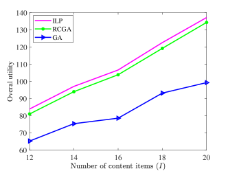
Figure 3: Impact of $I$ on utility when $T=10$, $L=0.3\sum_{i\in\mathcal{I}}s_{i}$, and $C=0.5\sum_{i\in\mathcal{I}}s_{i}$.

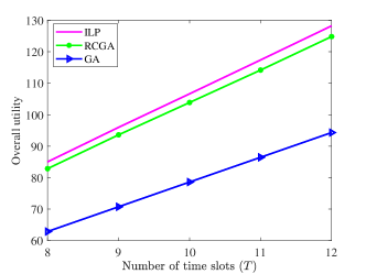
Figure 4: Impact of $T$ on utility when $I=16$, $L=0.3\sum_{i\in\mathcal{I}}s_{i}$, and $C=0.5\sum_{i\in\mathcal{I}}s_{i}$.

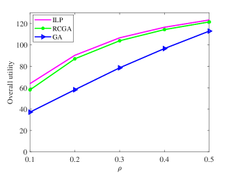
Figure 5: Impact of $\rho$ on utility when $I=16$, $T=10$, and $C=0.5\sum_{i\in\mathcal{I}}s_{i}$.

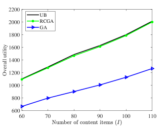
Figure 6: Impact of $I$ on utility when $T=24$, $L=0.3\sum_{i\in\mathcal{I}}s_{i}$, and $C=0.5\sum_{i\in\mathcal{I}}s_{i}$.

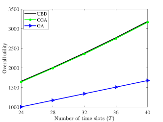
Figure 7: Impact of $T$ on utility when $I=90,L=0.3\sum_{i\in\mathcal{I}}s_{i}$, and $C=0.5\sum_{i\in\mathcal{I}}s_{i}$.

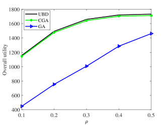
Figure 8: Impact of $\rho$ on utility when $I=90$, $T=24$, and $C=0.5\sum_{i\in\mathcal{I}}s_{i}$.

The results in Figs. 6-8 follow the same trend as the first three performance figures. Interestingly, for large-size ACOP instances, RCGA delivers better performance, as the achieved utility by RCGA virtually overlaps with UBD. We believe this is an effect of the knapsack structure of ACOP. When the number of content items is small, even few sub-optimal caching and updating decisions made by RCGA has noticeable impact on the overall sub-optimality. This is of less an issue with many content items. GA, however, has a worse performance for larger-size problem instances. The observation demonstrates the strength of RCGA over the simple greedy schedule. Finally, our performance evaluation using the UBD is accurate, because the global optimum is between the utility by RCGA and the UBD that are almost overlapping.

8 Extension to Cyclic Schedule

Suppose the caching and updating schedule is cyclic. Namely, the schedule repeats itself for every $T$ time slots. Hence the AoI of an item in time slot one depends on the scheduling decisions made for the item in later time slots. In this section, we discuss applying our results and algorithmic notions to cyclic schedule.

The NP-hardness of cyclic scheduling clearly remains, as the proof of Theorem 1 applies directly. For uniform item size, the polynomial-time tractability stated in Theorem 4 can be generalized to cyclic schedule based on the notion of flow circulation, which refers to a flow pattern satisfying flow balance at every node of a graph without source or destination nodes. We modify the network graph (in Fig. 1) such that the last node $n_{T}$ coincides with the first node $n_{0}$. Moreover, each node $n_{i},i=1,\dots,T-1$ is split into two nodes $n_{i}$ and $n^{\prime}_{i}$ connected by a single arc $(n_{i},n^{\prime}_{i})$ of tuple $(0,I,I)$, i.e., there will be exactly $I$ flow units on this arc for every time slot. Finding the optimal cyclic schedule corresponds then to solving the minimum-cost circulation flow problem for which the optimum can be computed in polynomial time (e.g., [39]).

Adapting the ILP formulation in Section 5 to cyclic scheduling is easy; this amounts to adding an additional constraint of type (1) to connect together time slots $1$ and $T$. The reformulation (2) and our algorithm RCGA remain applicable. The difference from acyclic schedule lies in the subproblem. Namely, instead of finding a shortest path with graph construction shown in Fig. 2, the subproblem consists in finding minimum cost circulation in a modified graph as discussed above.

Finally, we remark that the underlying rationale of the greedy solution in Section 3.2 does not appear very logical for a cyclic schedule. The greedy algorithm works slot by slot, and, for each slot, the algorithm uses the AoI values of the previous slot as input. With cyclic scheduling, this input is not available as it depends on the whole scheduling solution. Nevertheless, the greedy acyclic schedule is still a valid solution to be used as a cyclic schedule, though the true utility values need to be evaluated afterward.

9 Conclusions

We have considered the optimization problem of time-dynamic caching where the performance metric is age-centric. Our work has led to the following key findings. First, the problem complexity originates from the knapsack structure, whereas for uniform item size it is polynomial-time solvable. These results settle the boundary of problem tractability. Second, column generation offers an effective approach for problem solving in terms of obtaining clear-optimal solutions. As another concluding remark, we believe our results and algorithm admit extensions to a couple of other related performance functions. One is time-specific utility function as the popularity of content items may change over time. The other is the minimization of average AoI.

References

- [1] S. Kaul, R. D. Yates, and M. Gruteser, “Real-time status: How often should one update?” in Proc. of IEEE INFOCOM, 2012, pp. 2731–2735.
- [2] R. D. Yates, P. Ciblat, A. Yener, and M. Wigger, “Age-optimal constrained cache updating,” in Proc. of IEEE ISIT, 2017, pp. 2157–8117.
- [3] R. D. Yates and S. Kaul, “Real-time status updating: multiple sources,” in Proc. of IEEE ISIT, 2012, pp. 2666–2670.
- [4] C. Kam, S. Kompella, and A. Ephremides, “Age of information under random updates,” in Proc. of IEEE ISIT, 2013, pp. 66–70.
- [5] M. Costa, M. Codreanu, and A. Ephremidesy, “Age of information with packet management,” in Proc. of IEEE ISIT, 2014, pp. 1583–1587.
- [6] N. Pappas, J. Gunnarsson, L. Kratz, M. Kountouris, and V. Angelakis, “Age of information of multiple sources with queue management,” in Proc. of IEEE ICC, 2015.
- [7] M. Costa, S. Valentin, and A. Ephremides, “First steps to understand the age of channel information,” in Proc. of 1st KuVS Workshop on Anticipatory Networks, 2014, pp. 4–6.
- [8] R. D. Yates, “Lazy is timely: Status updates by an energy harvesting source,” in Proc. of IEEE ISIT, 2015, DOI:10.1109/ISIT.2015.7283009.
- [9] Y. Sun, E. Uysal-Biyikoglu, R. D. Yates, C. E. Koksal, and N. B. Shroff, “Update or wait: How to keep your data fresh,” IEEE Transactions on Information Theory, vol. 63, pp. 7492–7508, 2017.
- [10] Y. Sang, B. Li, and B. Ji, “The power of waiting for more than one response in minimizing the age-of-information,” in Proc. of IEEE GLOBECOM, 2017.
- [11] I. Kadota, E. Uysal-Biyikoglu, R. Singh, and E. Modiano, “Minimizing the age of information in broadcast wireless networks,” in Proc. of IEEE Allerton, 2016, pp. 844–851.
- [12] Q. He, D. Yuan, and A. Ephremides, “Optimal link scheduling for age minimization in wireless systems,” IEEE Transactions on Information Theory, vol. 64, pp. 5381–5394, 2018.
- [13] A. Kosta, N. Pappas, and V. Angelakis, “Age of information: A new concept, metric, and tool,” Foundations and Trends® in Networking, vol. 12, pp. 162–259, 2017.
- [14] Y. Sun, E. Uysal-Biyikoglu, and S. Kompella, “Age-optimal updates of multiple information flows,” in Proc. of IEEE INFOCOM Workshops, 2018, DOI:10.1109/INFCOMWw.2018.8406945.
- [15] C. Kam, S. Kompella, G. Nguyen, J. Wieselthier, and A. Ephremides, “Towards an effective age of information: remote estimation of a Markov source,” in Proc. of IEEE INFOCOM Workshops, 2018, DOI:10.1109/INFCOMW.2018.8406891.
- [16] J. Sun, Z. Jiang, S. Zhou, and Z. Niu, “Optimizing information freshness in broadcast network with unreliable links and random arrivals: an approximate index policy,” in Proc. of IEEE INFOCOM Workshops, 2019.
- [17] S. Farazi, A. G. Klein, and D. R. Brown III, “Average age of information for status update systems with an energy harvesting server,” in Proc. of IEEE INFOCOM Workshops, 2018, DOI:10.1109/INFCOMW.2018.8406846.
- [18] R. D. Yates, “Age of information in a network of preemptive servers,” in Proc. of IEEE INFOCOM Workshops, 2018, DOI:10.1109/INFCOMW.2018.8406966.
- [19] E. Najm and E. Telatar, “Status updates in a multi-stream M/G/1/1 preemptive queue,” in Proc. of IEEE INFOCOM Workshops, 2018, DOI:10.1109/INFCOMW.2018.8406928.
- [20] X. Wang and L. Duan, “Dynamic pricing for controlling age of information,” in Proc. of IEEE INFOCOM Workshops, 2019.
- [21] J. P. Champsti, M. H. Mamduhi, K. H. Joansson, and J. Gross, “Performance characterization using aoi in a single-loop networked control system,” in Proc. of IEEE INFOCOM Workshops, 2019.
- [22] M. Klugel, M. H. Mamduhi, S. Hiche, and W. Kellerer, “AoI-penalty minimization for networked control systems with packet loss,” in Proc. of IEEE INFOCOM Workshops, 2019.
- [23] Q. He, G. Dán, and V. Fodor, “On emptying a wireless network with minimum-energy under age constraints,” in Proc. of IEEE INFOCOM Workshops, 2019.
- [24] S. Farazi, A. G. Klein, and D. R. Brown III, “Fundamental bounds on the age of information in general multi-hop interference networks,” in Proc. of IEEE INFOCOM Workshops, 2019.
- [25] Y. Dong, Z. Chen, and P. Fan, “Uplink age of information of unilaterally powered two-way data exchanging systems,” in Proc. of IEEE INFOCOM Workshops, 2018, DOI: 10.1109/INFCOMW.2018.8407009.
- [26] Q. He, G. Dán, and V. Fodor, “Minimizing age of correlated information for wireless camera networks,” in Proc. of IEEE INFOCOM Workshops, 2018, DOI:10.1109/INFCOMW.2018.8406914.
- [27] J. Liu, X. Wang, B. Bai, and H. Dai, “Age-optimal trajectory planning for UAV-assisted data collection,” in Proc. of IEEE INFOCOM Workshops, 2018, DOI:10.1109/INFCOMW.2018.8406973.
- [28] J. Zhong, R. Yates, and E. Soljanin, “Minimizing content staleness in dynamo-style replicated storage systems,” in Proc. of IEEE INFOCOM Workshops, 2018, DOI:10.1109/INFCOMW.2018.8406971.
- [29] A. Maatouk, M. Assaad, and A. Ephremides, “Minimizing the age of information: NOMA or OMA?” in Proc. of IEEE INFOCOM Workshops, 2019.
- [30] E. T. Ceran, D. Gündüz, and A. György, “A reinforcement learning approach to age of information in multi-user networks,” in Proc. of IEEE PIMRC, 2018, DOI:10.1109/PIMRC.2018.8580701.
- [31] C. Kam, S. Kompella, and A. Ephremides, “Learning to sample a signal through an unknown system for minimum AoI,” in Proc. of IEEE INFOCOM Workshops, 2019.
- [32] H. Tang, P. Ciblat, J. Wang, M. Wigger, and R. Yates, “Age of information aware cache updating with file- and age-dependent update durations,” https://arxiv.org/pdf/1909.05930.pdf, 2019.
- [33] R. K. Ahuja, T. L. Magnanti, and J. B. Orlin, Network Flows: Theory, Algorithms, and Applications. Pearson Press, 2014.
- [34] GUROBI, “GUROBI Optimizer 8.1,” http://www.gurobi.com/, 2019.
- [35] M. Lubecke and J. Desrosiers, “Selected topics in column generation,” Operations Research, vol. 53, pp. 1007–1023, 2004.
- [36] M. Karamano and G. Cornuéjols, “Branching on general disjunctions,” Mathematical Programming, vol. 128, pp. 403–436, 2009.
- [37] Y. Sun and B. Cyr, “Sampling for data freshness optimization: Non-linear age functions,” Journal of Communications and Networks, vol. 21, no. 3, pp. 204–219, 2019.
- [38] S. Ioannidis, A. Chaintreau, and L. Massoulie, “Optimal and scalable distribution of content updates over a mobile social network,” in Proc. of IEEE INFOCOM, 2009, pp. 1422–1430.
- [39] É. Tardos, “A storngly polynomial minimum cost circulation algorithm,” Combinatorica, vol. 5, pp. 247–255, 1985.