Search for lepton flavour violating muon decay mediated by a new light particle in the MEG experiment

Abstract

We present the first direct search for lepton flavour violating muon decay mediated by a new light particle X, $\muup^{+}\to\mathrm{e}^{+}\mathrm{X},\mathrm{X}\to\gammaup\gammaup$. This search uses a dataset resulting from $7.5\times 10^{14}$ stopped muons collected by the MEG experiment at the Paul Scherrer Institut in the period 2009–2013. No significant excess is found in the mass region 20–45 MeV/c² for lifetimes below 40 ps, and we set the most stringent branching ratio upper limits in the mass region of 20–40 MeV/c², down to $\mathcal{O}(10^{-11})$ at 90% confidence level.

1 Introduction

The search for charged lepton flavour violating (CLFV) processes is one of the key tools to probe for physics beyond the Standard Model (SM) of elementary particles and interactions. The observation of neutrino oscillationsSK:1998 ; SNO:2002 ; PDG2018 showed that lepton flavour is not conserved in nature. As a consequence, charged lepton flavour is violated, even though the rate is unobservably small ($<\!10^{-50}$) in an extension of the SM accounting for measured neutrino mass differences and mixing angles Petcov:1977 ; Cheng:1980 . In the context of new physics, in the framework of grand unified theories for example, CLFV processes can occur at an experimentally observable rate barbieri1994 . Therefore, such processes are free from SM physics backgrounds and a positive signal would constitute unambiguous evidence for physics beyond the SM. This motivates the effort to search for evidence of new physics through CLFV processes mori_2014 ; calibbi_2018 .

The MEG experiment at the Paul Scherrer Institut (PSI) in Switzerland searched for one such CLFV process, $\muup^{+}\to\mathrm{e}^{+}\gammaup$ decay, with the highest sensitivity in the world. No evidence of the decay was found yet, leading to an upper limit on the branching ratio $\mathcal{B}(\muup^{+}\to{\rm e}^{+}\gammaup)<4.2\times 10^{-13}$ at 90% confidence level (C.L.) baldini_2016 . Models that allow $\muup^{+}\to\mathrm{e}^{+}\gammaup$ decay at an observable rate usually assume that CLFV couplings are introduced through an exchange of new particles much heavier than the muon. Negative results by CLFV searches leave open another possibility: new physics exists at a lighter scale but with very weak coupling to SM particles.

If a new particle X (with mass $m_{\mathrm{X}}$ and lifetime $\tau_{\mathrm{X}}$) lighter than the muon exists, the CLFV two-body decay $\muup\to\mathrm{eX}$ may be a good probe for such new physics. The experimental signature depends on how the new particle X decays. In this paper, we report a search for $\muup^{+}\to\mathrm{e}^{+}\mathrm{X},\mathrm{X}\to\gammaup\gammaup$ (MEx2G) decay using the full dataset collected in the MEG experiment. Here, we assume that X is an on-shell scalar or pseudo-scalar particle. Axion-like particles Peccei1977 ; Weinberg1978 ; Wilczek1978 ; Cornella2019 , Majoron Chikashige1981 ; Gelmini1981 , familon Reiss1982 ; Wilczek1982 ; Berezhiani1990 ; Jaeckel2014 , flavon Tsumura2010 ; Bauer2016 , flaxion Ema2017 ; calibbi_2017 , hierarchion Davidi2018 , and strongly interacting massive particles Hochberg2014 ; Hochberg2015 are candidates for X.

A dedicated search for the MEx2G decay has never been done, although some constraints on the X particle parameter space can be deduced by experimental results from both related muon decay modes and non-muon experiments; these are discussed below.

Current upper limits on the inclusive decay $\muup^{+}\to\mathrm{e^{+}X}$ are given at $\mathcal{O}(10^{-5})$ for $m_{\mathrm{X}}$ in the range 13–80 MeV/c² Bayes2015 . However, the current limits do not impose any constraints on the MEx2G decay in the target region of this search. They are complementary, relevant for cases where X is either stable or decays invisibly. For X resulting from muon decays, the only kinematically allowed visible decay channels are $\mathrm{X\to e^{+}e^{-}}$ and $\mathrm{X}\to\gammaup\gammaup$. The former can occur at tree level while the latter can occur via a fermion loop. The current upper limit on $\muup^{+}\to\mathrm{e^{+}X},\mathrm{X}\to\mathrm{e^{+}e^{-}}$ at a level of $\mathcal{O}(10^{-12})$ Eichler1986 give stringent constraints on the MEx2G decay if we assume that X is more likely to decay into an e⁺e^- pair. However, there is a possibility for X to be electrophobic, as pointed out in Anderson2003 ; Liu2016 , and searches for both decay modes can hint at the model behind these decay modes.

The current upper limit on the decay $\muup^{+}\rightarrow\mathrm{e^{+}}\gammaup\gammaup$, $\mathcal{B}(\muup^{+}\rightarrow\mathrm{e^{+}}\gammaup\gammaup)<7.2\times 10^{-11}$ (90% C.L.) from the Crystal Box experiment bolton_1988_prd can be converted into an equivalent MEx2G upper limit by taking into account the difference in detector efficiencies Natori2012 ; the converted limits are shown in Fig. 1.

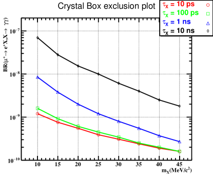
Figure 1: Upper limits on MEx2G decay estimated by converting the upper limits on $\muup^{+}\rightarrow\mathrm{e^{+}}\gammaup\gammaup$ from the Crystal Box experiment as a function of $m_{\mathrm{X}}$. Lines with different markers and colours correspond to different $\tau_{\mathrm{X}}$.

Axion-like particle searches from collider and beam dump experiments and from supernova observations also constrain the branching ratio $\mathrm{X}\rightarrow\gammaup\gammaup$ if the axion-like particles are generated from coupling to photons Heeck2018 . Figure 2 summarises the parameter regions excluded by these experiments. A region with decay length c$\tau_{\rm{X}}\gamma<$ 1 cm and $m_{\rm{X}}>20$ MeV/c² still has room for the MEx2G decay.

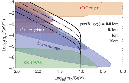
Figure 2: Excluded parameter regions for a scalar X with mass $m_{\rm{X}}$ and coupling $g_{\gamma\gamma}$ to 2$\gammaup$s from collider, beam dumps, and supernova Dolan2017 ; Dobrich2016 ; Jaeckel2016 (from Heeck2018 ). In black we show contours of the boosted decay length $\gamma\mathrm{c}\tau_{\mathrm{X}}$ of $\mathrm{X}\rightarrow\gammaup\gammaup$, assuming X to be produced from an at-rest muon decay $\muup^{+}\to\mathrm{e^{+}X}$. The solid black line corresponds to $\gamma\mathrm{c}\tau_{\mathrm{X}}=0.01$ cm, the dotted one to 0.1 cm, the dashed one to 1 cm and the dot-dashed line to 10 cm.

Based on limits discussed above, we define the target parameter space of this search in the $\tau_{\mathrm{X}}$–$m_{\mathrm{X}}$ plane as shown in Fig. 3.

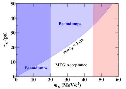
Figure 3: Allowed X particle parameter space (white). The blue region has already been excluded Dobrich2016 and the red shaded region on the right ($m_{\mathrm{X}}\gtrsim 45$ MeV/c²) is inaccessible to MEG.

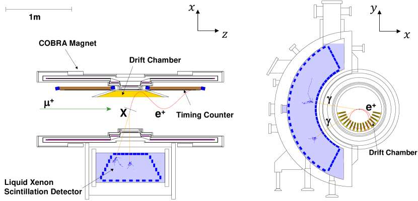
Figure 4: The figure shows a schematic view of the MEG detector with a simulated MEx2G event emitted from the target. The top view is shown on the left, the view from downstream on the right.

2 Detector

The MEG detector is briefly presented in the following, emphasising aspects relevant to this search; a detailed description is available in megdet .

In this paper we adopt a Cartesian coordinate system $(x,y,z)$ shown in Fig. 4 with the origin at the centre of the magnet. When necessary, we also refer to the cylindrical coordinate system ${\it(r,\phi,z)}$ as well as the polar angle $\theta$.

Multiple intense $\muup^{+}$ beams are available at the $\piup$E5 channel in the 2.2-mA PSI proton accelerator complex. We use a beam of surface muons, produced by $\piup^{+}$ decaying near the surface of a production target. The beam intensity is tuned to a $\muup^{+}$ stopping rate of $3\times 10^{7}$, limited by the rate capabilities of the tracking system and the rate of accidental backgrounds in the $\muup^{+}\to\mathrm{e}^{+}\gammaup$ search. The muons at the production target are fully polarised ($P_{\muup^{+}}=-1$), and they reach a stopping target with a residual polarisation $P_{\muup^{+}}=-0.86\pm 0.02\leavevmode\nobreak\ {\rm(stat)}\leavevmode\nobreak\ {}^{+0.05}_{-0.06}\leavevmode\nobreak\ {\rm(syst)}$ Baldini:2015lwl .

The positive muons are stopped and decay in a thin target placed at the centre of the spectrometer at a slant angle of $\approx$ $20^{\circ}$ from the $\muup^{+}$ beam direction. The target is composed of a 205 $\muup$m thick layer of polyethylene and polyester (density $0.895$ g/cm³).

Positrons from the muon decays are detected with a magnetic spectrometer, called the COBRA (standing for COnstant Bending RAdius) spectrometer, consisting of a thin-walled superconducting magnet, a drift chamber array (DCH), and two scintillating timing counter (TC) arrays.

The magnet Ootani2004 is made of a superconducting coil with three different radii. It generates a gradient magnetic field of 1.27 T at the centre and 0.49 T at each end. The diameter of an emitted e⁺ trajectory depends on the absolute momentum, independent of the polar angle due to the gradient field. This allows us to select e⁺s within a specific momentum range by placing the TC detectors in a specific radial range; e⁺s whose momenta are larger than $\sim$45 MeV/c fall into the acceptance of the TC. Furthermore, the gradient field prevents e⁺s emitted nearly perpendicular to the $\muup^{+}$ beam direction from looping many times in the spectrometer. This results in a suppression of hit rates in the DCH. The thickness of the central part of the magnet is 0.2 radiation length to maximise transparency to $\gammaup$; 85% of the signal $\gammaup$s penetrate the magnet without interaction and reach the photon detector.

Positrons are tracked in the DCH Hildebrandt2010 . It is composed of 16 independent modules. Each module has a trapezoidal shape with base lengths of 104 cm (at smaller radius, close to the stopping target) and 40 cm (at larger radius). These modules are installed in the bottom hemisphere in the magnet at 10.5^∘ intervals. The DCH covers the azimuthal region between 191.25^∘ and 348.75^∘ and the radial region between 19.3 cm and 27.9 cm. It is composed of low mass materials and helium-based gas ($\mathrm{He}:\mathrm{C_{2}H_{6}}=1:1$) to suppress Coulomb multiple scattering; $2.0\times 10^{-3}$ radiation length path is achieved for the e⁺ from $\muup^{+}\to\mathrm{e}^{+}\gammaup$ decay at energy of $E_{\mathrm{e^{+}}}=52.83$ MeV ($=m_{\muup}\mathrm{c}^{2}/2$, where $m_{\muup}$ is the mass of muon).

The TC DeGerone2011 ; DeGerone2012 is designed to measure precisely the e⁺ hit time. Fifteen scintillator bars are placed at each end of the COBRA. They are made of $4\times 4\times 80$ cm³ plastic scintillators with fine-mesh PMTs attached to both ends of the bars.

The efficiency of the spectrometer significantly depends on $E_{\mathrm{e^{+}}}$ as shown in Fig. 5. The e⁺ energy from the MEx2G decay is lower than that from $\muup^{+}\to\mathrm{e}^{+}\gammaup$ depending on $m_{\mathrm{X}}$, and the efficiency is correspondingly lower. The large $m_{\mathrm{X}}$ search range is limited by this effect as shown in Fig. 3.

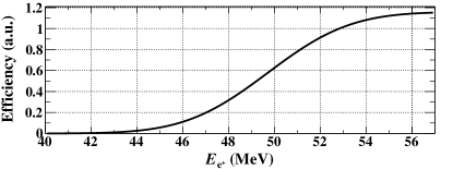
Figure 5: COBRA spectrometer relative efficiency as a function of $E_{\mathrm{e^{+}}}$ normalised to $\epsilon_{\mathrm{e^{+}}}(52.83$ MeV) = 1.

The photon detector is a homogeneous liquid-xenon (LXe) detector relying on scintillation light for energy, position, and timing measurement Sawada2010258 ; baldini_2005_nim . As shown in Fig. 4, it has a C-shaped structure fitting the outer radius of the magnet. The fiducial volume is $\approx$ 800 $\ell$, covering 11% of the solid angle viewed from the centre of the stopping target in the radial range of $67.85<r<105.9$ cm, corresponding to $\approx 14$ radiation length. It is able to detect a 52.83-MeV $\gammaup$ with high efficiency and to contain the electromagnetic shower induced by it. The scintillation light is detected by 846 2-inch PMTs submerged directly in the liquid xenon. They are placed on all six faces of the detector, with different PMT coverage on different faces. On the inner face, which is the densest part, the PMTs align at intervals of 6.2 cm.

One of the distinctive features of the MEG experiment is that it digitises and records all waveforms from the detectors using the Domino Ring Sampler v4 (DRS4) chip Ritt2010 . The sampling speeds are set to 1.6 GSPS for TC and LXe photon detector and 0.8 GSPS for DCH. This lower value for DCH is selected to match the drift velocity and the required precision.

The DAQ event rate was kept below 10 Hz in order to acquire the full waveform data ($\approx$ 1 MB/event). It was accomplished using a highly efficient online trigger system trigger2013 ; Galli:2014uga .

Several types of trigger logic were implemented and activated during the physics data-taking each with its own prescaling factor. However, a dedicated trigger for the MEx2G events was neither foreseen nor implemented. Thus, we rely on the $\muup^{+}\to\mathrm{e}^{+}\gammaup$ triggered data in this search.

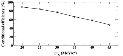
Figure 6: Trigger direction match efficiency for the MEx2G decay conditional to $\mathrm{e^{+}}$ and $2\gammaup$ detection as a function of $m_{\mathrm{X}}$ evaluated with a Monte Carlo simulation (Sect. 4).

The main $\muup^{+}\to\mathrm{e}^{+}\gammaup$ trigger, with a prescaling of 1, used the following observables: $\gammaup$ energy, time difference between e⁺ and $\gammaup$, and relative direction of e⁺ and $\gammaup$. The DC was not used in the trigger due to the slow drift velocity. The condition on the relative direction is designed to select back-to-back events. To calculate the relative direction, the PMT that detects the largest amount of scintillation light is used for the $\gammaup$, while the hit position at the TC is used for the e⁺. This direction match requirement results in inefficient selection of the MEx2G signal because, unlike the $\muup^{+}\to\mathrm{e}^{+}\gammaup$ decay, the MEx2G decay has 2$\gammaup$s with a finite opening angle, resulting in events often failing to satisfy the direction trigger. The selection inefficiency for MEx2G events is 10–50% depending on $m_{\mathrm{X}}$ as shown in Fig. 6.

Finally, the detector has been calibrated and monitored over all data-taking period with various methods calibration_cw ; papa_2007 , ensuring that the detector performances have been under control over the duration of the experiment.

3 Search strategy

The MEx2G signal results from the sequential decays of $\muup^{+}\to\mathrm{e^{+}}\mathrm{X}$ followed by $\mathrm{X}\to\gammaup\gammaup$. The first part is a two-body decay of a muon at rest, signalled by a mono-energetic e⁺. The energy $E_{\mathrm{e^{+}}}$ is determined by $m_{\mathrm{X}}$: $E_{\mathrm{e^{+}}}(m_{\mathrm{X}}=0)=52.83$ MeV and is a decreasing function of $m_{\mathrm{X}}$. The sum of energies of the two $\gammaup$s is also mono-energetic and an increasing function of $m_{\mathrm{X}}$. The momenta of the two $\gammaup$s are Lorentz-boosted along the direction of X, which increases the acceptance in the LXe photon detector compared to the three-body decay $\muup^{+}\to\mathrm{e^{+}}\gammaup\gammaup$. The final-state three particles is expected to have an invariant mass of 105.7 MeV$/\mathrm{c}^{2}(=m_{\muup})$ and the total momentum vector equal to 0.

A physics background that generates time-coincident $\mathrm{e^{+}}\gammaup\gammaup$ in the final state is $\muup^{+}\to{\rm e}^{+}\nuup\bar{\nuup}\gammaup\gammaup$. This mode has not yet been measured but exists in the SM. The branching ratio is calculated to be $\sim\mathcal{O}(10^{-14})$ for the MEG detector configuration without any cut on $E_{\mathrm{e^{+}}}$  Pruna:2017upz ; Banerjerr:2020 . Therefore, its contribution is certainly negligible in this search where we apply cuts on $E_{\mathrm{e^{+}}}$.

The dominant background is the accidental pileup of multiple $\muup^{+}$s decays. There are three types of accidental background events:

Type 1:

The e⁺ and one of the $\gammaup$s originate from one $\muup^{+}$, and the other $\gammaup$ from a different one.

Type 2:

The two $\gammaup$s share the same origin, and the e⁺ is accidental.

Type 3:

All the particles are accidental.

The main source of a time-coincident $\mathrm{e^{+}}\gammaup$ pair in type 1 is the radiative muon decay $\muup^{+}\to\mathrm{e}^{+}\nuup\bar{\nuup}\gammaup$ megrmd . The sources of time-coincident $\gammaup\gammaup$ pairs in type 2 are $\mathrm{e}^{+}\mathrm{e}^{-}\to\gammaup\gammaup$ (e⁺ from $\muup^{+}$ decay and e^- from material along the e⁺ trajectory), $\muup^{+}\to\mathrm{e}^{+}\nuup\bar{\nuup}\gammaup$ with an additional $\gammaup$, e.g. by a bremsstrahlung from the e⁺, or a cosmic-ray induced shower.

Figure 7 shows the decay kinematics and the kinematic variables. The muon decay vertex and the momentum of the e⁺ are obtained by reconstructing the e⁺ trajectory using the hits in DCH and TC and the intersection of the trajectory with the plane of the muon beam stopping target (Sect. 5.1). The interaction positions and times of the two $\gammaup$s within the LXe photon detector and their energies are individually reconstructed using the PMT charge and time information of the LXe photon detector (Sect. 5.2).

Given the muon decay vertex, the two $\gammaup$s’ energies and positions, and $m_{\mathrm{X}}$, the X decay vertex $\mbox{\boldmath$x$}_{\mathrm{vtx}}$ can be computed. Therefore, we reconstruct $\mbox{\boldmath$x$}_{\mathrm{vtx}}$ by scanning the assumed value of $m_{\mathrm{X}}$ (Sect. 5.3.1). If the final-state three particles do not originate at a single muon decay vertex, these variables will be inconsistent with originating from a single point. After reconstructing $\mbox{\boldmath$x$}_{\mathrm{vtx}}$, the relative time and angles (momenta) between X and e⁺ are tested for consistency with a muon decay (Sect. 5.3.2 and 5.3.3).

The MEx2G decay search analysis is performed within the mass range 20 MeV/c${}^{2}<m_{\mathrm{X}}<45\leavevmode\nobreak\$MeV/c² at 1 MeV/c² step. This step is chosen small enough not to miss signals in the gaps. Therefore, adjacent mass bins are not statistically independent. The analysis was performed assuming lifetimes $\tau_{\mathrm{X}}=5,20$, and $40$ ps; the value affects only the signal efficiency.

We estimate the accidental background by using the data in which the particles are not time coincident. To reduce the possibility of experimental bias, a blind analysis is adopted; the blind region is defined in the plane of the relative times of the three particles (Sect. 6).

The signal efficiency is evaluated on the basis of a Monte Carlo simulation (Sect. 4). Its tuning and validation are performed using pseudo-2$\gammaup$ data as described in Sect. 4.1.

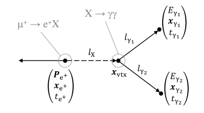
Figure 7: Decay kinematics and kinematic variables.

4 Simulation

The technical details of the program of Monte Carlo (MC) simulation are presented in softwaretns and an overview of the physics and detector simulation is available in megdet . In the following we report a brief summary.

The first step of the simulation is the generation of the physics events. That is realised with custom written code for a large number of relevant physics channels. The MEx2G decay is simulated starting from a muon at rest in the target; the decay products are generated in accordance with the decay kinematics for the given $m_{\mathrm{X}}$ and $\tau_{\mathrm{X}}$.

The muon beam transport, interaction in the target, and propagation of the decay products in the detector are simulated with a MC program based on GEANT3.21 GEANT3 that describes the detector response. Between the detector simulation and the reconstruction program, an intermediate program processes the MC information, adding readout simulation and allowing event mixing to study the detector performance under combinatorial background events. Particularly, the $\muup^{+}$ beam, randomly distributed in time at a decay rate of $3\times 10^{7}\leavevmode\nobreak\ \muup^{+}\mathrm{s^{-1}}$, is mixed with the MEx2G decay to study the e⁺ spectrometer performance. The detectors’ operating condition, such as the active layers of DCH and the applied high-voltages, are implemented with the known time dependence.

In order to simulate the accidental activity in the LXe photon detector, data collected with a random-time trigger are used. A MC event and a random-trigger event are overlaid by summing the numbers of photo-electrons detected by each PMT.

4.1 Pseudo two $\gammaup$ data

To study the performance of the 2$\gammaup$ reconstruction, we built pseudo 2$\gammaup$ events using calibration data. The following $\gammaup$-ray lines are obtained in calibration runs:

• 54.9 MeV and 82.9 MeV from $\piup^{-}\mathrm{p}\to\piup^{0}\mathrm{n}\to\gammaup\gammaup\mathrm{n}$ reaction,

• 17.6 MeV and 14.6 MeV from ${}^{7}\mathrm{Li}(\mathrm{p},\gammaup)^{8}\mathrm{Be}$ reaction,

• 11.7 MeV from ${}^{11}\mathrm{B}(\mathrm{p},2\gammaup)^{12}\mathrm{C}$ reaction.

The selection criteria for those calibration events are detailed in calibration_cw and Adam2013 . We take two events from the above calibration data and overlay them, summing the number of photo-electrons PMT by PMT. These pseudo 2$\gammaup$ events are generated using both data and MC events.

5 Event reconstruction

We describe here the reconstruction methods and their performance, focusing on high-level objects; descriptions of the manipulation of low-level objects, including waveform analysis and calibration procedures, are available in baldini_2016 ; megdet . The e⁺ reconstruction (Sect. 5.1) is identical to that used in the $\muup^{+}\to\mathrm{e}^{+}\gammaup$ decay analysis in baldini_2016 . The 2$\gammaup$ reconstruction was developed originally for this analysis (Sect. 5.2). After reconstructing the e⁺ and two $\gammaup$s, the reconstructed variables are combined to reconstruct the X decay vertex (Sect. 5.3).

5.1 Positron reconstruction

Positron trajectories in the DCH are reconstructed using the Kalman filter technique Billoir1984 ; Fruhwirth1987 based on the GEANE software Fontana2008 . This technique takes the effect of materials into account. After the first track fitting in DCH, the track is propagated to the TC region to test matching with TC hits. The matched TC hits are connected to the track and then the track is refined using the TC hit time. Finally, the fitted track is propagated back to the stopping target, and the point of intersection with the target defines the muon decay vertex position ($\mbox{\boldmath$x$}_{\mathrm{e^{+}}}$) and momentum vector that defines the e⁺ emission angles ($\theta_{\mathrm{e^{+}}},\phi_{\mathrm{e^{+}}}$). The e⁺ emission time ($t_{\mathrm{e^{+}}}$) is reconstructed from the TC hit time minus the e⁺ flight time.

Positron tracks satisfying the following criteria are selected: the number of hits in DCH is more than six, the reduced chi-square of the track fitting is less than 12, the track is matched with a TC hit, and the track is successfully propagated back to the fiducial volume of the target. If multiple tracks in an event pass the criteria, only one track is selected and passed to the following analysis, based on the covariance matrix of the track fitting as well as the number of hits and the reduced chi-square.

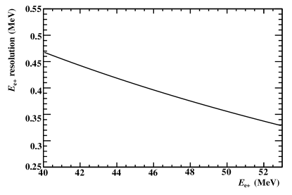
Figure 8: $E_{\mathrm{e^{+}}}$ resolution as a function of $E_{\mathrm{e^{+}}}$.

The resolutions are evaluated based on the MC, tuned to data using double-turn events; tracks traversing DCH twice (two turns) are selected and reconstructed independently by using hits belonging to each turn. The difference in the reconstruction results by the two turns indicates the resolution. The MC results are smeared so that the double-turn results become the same as those with the data. Figure 8 shows the $E_{\mathrm{e^{+}}}$ resolution as a function of $E_{\mathrm{e^{+}}}$. The angular resolutions also show a similar $E_{\mathrm{e^{+}}}$ dependence. The $\phi_{\mathrm{e^{+}}}$- and $\theta_{\mathrm{e^{+}}}$-resolutions for $m_{\mathrm{X}}=20\,(45)$ MeV/c² are $\sigma_{\phi_{\mathrm{e^{+}}}}\sim 12\,(15)$ mrad and $\sigma_{\theta_{\mathrm{e^{+}}}}\sim 10\,(11)$ mrad, respectively. The time resolution is $\sigma_{t_{\mathrm{e^{+}}}}\sim 100\,(130)$ ps.

5.2 Photon reconstruction

Coordinates $(u,v,w)$ are used in the LXe photon detector local coordinate system rather than the global coordinates $(x,y,z)$: $u$ coincides with $z$, $v=r_{\mathrm{in}}(\pi-\phi)$ where $r_{\mathrm{in}}=67.85$ cm is the radius of the inner face, and $w=r-r_{\mathrm{in}}$ is the depth measured from the inner face.

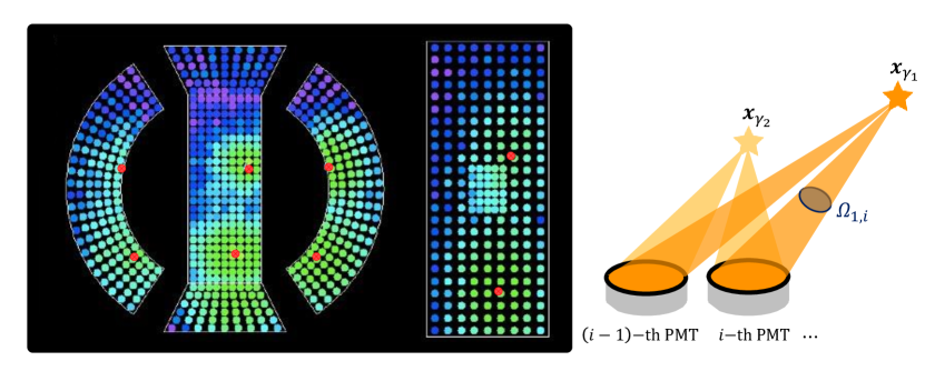
Figure 9: Event display of the LXe photon detector for a 2$\gammaup$ event (in a development view). The red points show the interaction positions of the two $\gammaup$s projected to each face. Each circular marker denotes a PMT. The colour indicates the measured light yield, which is the sum of photons from the two showers induced by the two $\gammaup$s as depicted in the right figure.

5.2.1 Multiple photon search

A peak search is performed based on the light distributions on the LXe photon detector inner and outer faces by using TSpectrum2 TSpectrum2 ; Morhac:2000 . The threshold of the peak light yield is set to 200 photons. Events that have more than one peak are identified as multiple-$\gammaup$ events.

5.2.2 Position and energy

Hereafter, only the multiple-$\gammaup$ events are analysed. When more than two $\gammaup$s are found, we select the two with the largest energy by performing the position-energy fitting described in this subsection on different combinations of two $\gammaup$s.

Figure 9 shows a typical event display of a 2$\gammaup$ event. Each PMT detects photons from the two $\gammaup$s. The key point of the 2$\gammaup$ reconstruction is how to divide the number of photons detected in each PMT into a contribution from each $\gammaup$.

Calculation of initial values

First, the positions of the detected peaks in ($u,v$) are used as the initial estimate with $w=1.5$ cm. Given the interaction point of each $\gammaup$ within the LXe photon detector, the contribution from each $\gammaup$ to each PMT can be calculated as follows. Assuming the ratio of the energy of $\gammaup_{1}$ to that of $\gammaup_{2}$ to be $E_{\gammaup_{1}}\colon E_{\gammaup_{2}}=R_{1}:(1-R_{1})$ ($0<R_{1}<1$, at first $R_{1}$ is set to 0.5), the fractions of the number of photons from $\gammaup_{1}$ is calculated as

$$R_{1,i}=\frac{R_{1}\Omega_{1,i}}{R_{1}\Omega_{1,i}+(1-R_{1})\Omega_{2,i}},$$ (1)

where $\Omega_{1,i}$ is the solid angle subtended by the $i$-th PMT from the $\gammaup_{1}$ interaction point. The total number of photons generated by $\gammaup_{1(2)}$, $M_{\mathrm{pho},1(2)}$, is calculated from the ratio $R_{1,i}$ and the number of photons at each PMT $N_{\mathrm{pho},i}$ as

$$M_{\mathrm{pho},1(2)}=\sum_{i}^{n_{\mathrm{{PMT}}}^{\mathrm{all}}}\left(R_{1,i}\times N_{\mathrm{pho},i}\right).$$ (2)

Then, $R_{1}$ is updated to $R_{1}=M_{\mathrm{pho},1}/(M_{\mathrm{pho},1}+M_{\mathrm{pho},2})$ and calculations (1) and (2) are repeated with the updated $R_{1}$. This procedure is iterated four times.

Position pre-fitting

Inner PMTs that detect more than 10 photons are selected to perform a position pre-fitting. The following quantity is minimised during the fitting:

$$\chi^{2}_{2\gammaup}=\sum_{i}^{n_{\mathrm{{PMT}}}^{\mathrm{selected}}}\frac{\left(N_{\mathrm{pho},i}-M_{\mathrm{pho},1}\Omega_{i}(\mbox{\boldmath$x$}_{\gammaup_{1}})-M_{\mathrm{pho},2}\Omega_{i}(\mbox{\boldmath$x$}_{\gammaup_{2}})\right)^{2}}{\sigma^{2}_{\mathrm{pho},i}(N_{\mathrm{pho},i})},$$ (3)

where $\sigma^{2}_{\mathrm{pho},i}(N_{\mathrm{pho},i})=N_{\mathrm{pho},i}/\epsilon_{\mathrm{PMT},i}$ with $\epsilon_{\mathrm{PMT},i}$ being the product of quantum and collection efficiencies of the PMT. This fitting is performed separately for each $\gammaup$: first, the light distribution is fitted with $\{\mbox{\boldmath$x$}_{\gammaup_{1}},M_{\mathrm{pho},1}\}$ as free parameters, while the other parameters are fixed; next, the light distribution is fitted with $\{\mbox{\boldmath$x$}_{\gammaup_{2}},M_{\mathrm{pho},2}\}$ as free parameters, while the other parameters are fixed.

Energy pre-fitting

To improve the energy estimation, $M_{\mathrm{pho},1(2)}$ are fitted while the other parameters are fixed. The same $\chi^{2}_{2\gammaup}$ (Eq. (3)) is used but only with PMTs that detect more than 200 photo-electrons.

The $\gammaup$ with the larger $M_{\mathrm{pho}}$ is defined as $\gammaup_{1}$ and the second largest one is defined as $\gammaup_{2}$ in the later analysis.

Position and energy fitting

At the final step, all the parameters are fitted simultaneously to eliminate the dependence of the fitted positions on the value of $M_{\mathrm{pho},1(2)}$ initially assumed. The best-fit value of $M_{\mathrm{pho},1(2)}$ is used to update $R_{1}$ and calculations (1) and (2) are repeated again to obtain the final value of $M_{\mathrm{pho},1(2)}$. Finally, it is converted into $E_{\gammaup_{1(2)}}$:

$$E_{\gammaup_{1(2)}} = U(\mbox{\boldmath$x$}_{\gammaup_{1(2)}})\times H(T)\times S\times M_{\mathrm{pho,1(2)}},$$ (4)

where $U(\mbox{\boldmath$x$}_{\gammaup_{1(2)}})$ is a uniformity correction factor, $H(T)$ is a time variation correction factor with $T$ being the calendar time when the event was collected, and $S$ is a factor to convert the number of photons to energy. The functions $U(\mbox{\boldmath$x$}_{\gammaup_{1(2)}})$ and $H(T)$ are mainly derived from the 17.6-MeV line from ${}^{7}\mathrm{Li}(\mathrm{p},\gammaup)^{8}\mathrm{Be}$ reaction, which was measured twice per week. The factor $S$ is calibrated using the 54.9-MeV line from $\piup^{0}$ decay, taken once per year.

Energy-ratio correction

Both the MC data and the pseudo-2$\gammaup$ data show an anti-correlation between the errors in $E_{\gammaup_{1}}$ and $E_{\gammaup_{2}}$ as shown in Fig. 10a, while their sum is not biased. Defining $R_{1}^{\mathrm{true}}$ as the $R_{1}$ for true energies for MC data and that for energies reconstructed without the overlay for real data, the reconstruction bias in both the MC data and the pseudo-2$\gammaup$ data is apparent by the linear dependence of $R_{1}/R_{1}^{\mathrm{true}}$ on $R_{1}$ as shown in Fig. 10b. This bias is removed by applying a correction to the reconstructed energies; the correction coefficients are evaluated from the pseudo-2$\gammaup$ data with different combinations of calibration data.

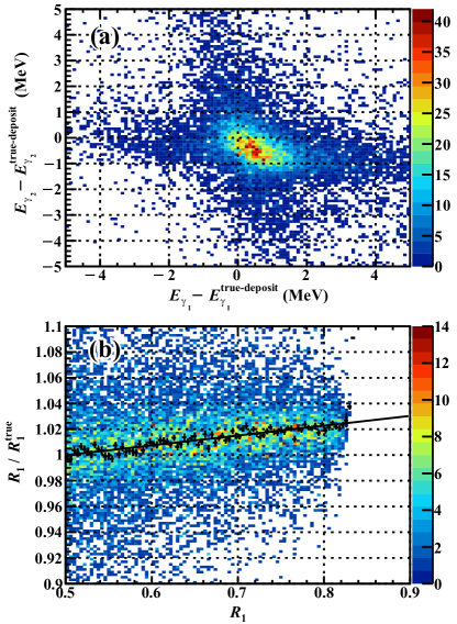
Figure 10: (a) Scatter plot of the energy reconstruction errors (MC). $E^{\mathrm{true-deposit}}_{\gammaup_{1(2)}}$ is the MC true value of the energy deposited in the LXe. (b) Dependence of the reconstructed energy ratio bias as a function of the reconstructed energy ratio (MC).

Position correction

Oblique incidence of $\gammaup$s to the inner face results in a bias of the fitted positions. This bias was checked and corrected for using the MC simulation. No bias is observed in the $v$ direction while a significant bias is observed in the $u$ direction. This is because the $\gammaup$s from the MEx2G decay enter the LXe photon detector almost perpendicularly in the $x$-$y$ view but enter with angles in the $z$-$r$ view. Since the $u$ bias arises from the direction and the size of the shower, it depends on the $u$ coordinate and the energy. Therefore, the correction function is prepared as a function of $u_{\gammaup_{1(2)}}$ and $E_{\gammaup_{1(2)}}$.

Selection criteria

To guarantee the quality of the reconstruction, the following criteria are imposed on the reconstruction results: the fits for both $\gammaup$s converge; the two $\gammaup$ positions are both within the detector fiducial volume defined as $|u|<25$ cm $\land$ $|v|<71$ cm; the distance between the two $\gammaup$s on the inner face is $d_{uv}>20$ cm; $E_{\gammaup_{1(2)}}>10$ MeV; and $E_{\gammaup_{1}}+E_{\gammaup_{2}}>40$ MeV.

Probability density function for $E_{\gammaup}$

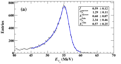
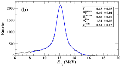
Figure 11: Energy response to MC $2\gammaup$ events with $E^{\mathrm{true}}_{\gammaup_{1}}=55$ MeV and $E^{\mathrm{true}}_{\gammaup_{2}}=12$ MeV. The blue curves are the PDFs fit to the distributions. See text for the formula of the PDFs.

The probability density function (PDF) for $E_{\gammaup_{1(2)}}$ is evaluated by means of the MC simulation. To tune the MC, the pseudo-2$\gammaup$ data of MC and data are used. It is asymmetric with a lower tail and modelled as follows:

$$P(E_{\gammaup}\mid E_{\gammaup}^{\mathrm{true}}) =f\cdot F(E_{\gammaup};E_{\gammaup}^{\mathrm{true}},E_{t}^{\mathrm{narrow}},\sigma_{E_{\gammaup}}^{\mathrm{narrow}})$$

$$+(1-f)\cdot F(E_{\gammaup};E_{\gammaup}^{\mathrm{true}},E_{t}^{\mathrm{wide}},\sigma_{E_{\gammaup}}^{\mathrm{wide}}),$$ (5)

where

$$F(E_{\gammaup};E_{\gammaup}^{\mathrm{true}},E_{t},\sigma_{E_{\gammaup}})$$

$$=\begin{cases}A\exp\left(-\frac{\left(E_{\gammaup}-E_{\gammaup}^{\mathrm{true}}\right)^{2}}{2\sigma^{2}_{E_{\gammaup}}}\right)&E_{\gammaup}>E_{\gammaup}^{\mathrm{true}}-E_{t}\\ A\exp\left(\frac{E_{t}}{\sigma^{2}_{E_{\gammaup}}}\left(\frac{E_{t}}{2}+(E_{\gammaup}-E_{\gammaup}^{\mathrm{true}})\right)\right)&E_{\gammaup}\leq E_{\gammaup}^{\mathrm{true}}-E_{t}\end{cases},$$ (6)

$E_{\gammaup}$ is a reconstructed $\gammaup$ energy, $E_{\gammaup}^{\mathrm{true}}$ is the true value, $f$ is the fraction of the narrow component, $A$ is a normalisation parameter, $E_{t}$ is the transition parameter between the Gaussian and exponential components, and $\sigma_{E_{\gammaup}}$ is the standard deviation of the Gaussian component describing the width on the high-energy side. The parameters $E_{t}$ and $\sigma_{E_{\gammaup}}$ are correlated with each other, different for the narrow and wide components, and are dependent on $E_{\gammaup}^{\mathrm{true}}$. Figure 11 shows an example of the PDFs for $2\gammaup$ events with $E^{\mathrm{true}}_{\gammaup_{1}}=55$ MeV and $E^{\mathrm{true}}_{\gammaup_{2}}=12$ MeV.

Probability density functions for $\gammaup$ position

The PDFs of $\gammaup$ position are almost independent of $E_{\gammaup_{1(2)}}$ and hence $(m_{\mathrm{X}},\tau_{\mathrm{X}})$. They are represented by double Gaussians with fractions of tail components of $\sim\!20$%. The standard deviations of the core components are $\mbox{\boldmath$\sigma$}^{\mathrm{core}}_{\mbox{\boldmath$x$}_{\gammaup_{1(2)}}}=(5.4,4.7,6.5)$ mm in $(u,v,w)$ coordinates, those of the tail components are $\mbox{\boldmath$\sigma$}^{\mathrm{tail}}_{\mbox{\boldmath$x$}_{\gammaup_{1(2)}}}=(29,19,45)$ mm.

5.2.3 Time

The interaction time of $\gammaup_{1}(\gammaup_{2})$ can be reconstructed using the pulse time measured by each PMT ($t_{\mathrm{PMT},i}$) by correcting for a delay time ($t_{\mathrm{delay},\gammaup_{1(2)},i}$) including the propagation time of the light between the interaction point and the PMT and the time-walk effect, and a time offset due to the readout electronics ($t_{\mathrm{offset},i}$):

$$t_{\gammaup_{1(2)},i}=t_{\mathrm{PMT},i}-t_{\mathrm{delay},\gammaup_{1(2)},i}-t_{\mathrm{offset},i}.$$ (7)

The single PMT time resolution $\sigma_{t,i}$ is approximately proportional to $1/\sqrt{N_{\mathrm{pe},\gammaup_{1(2)},i}}$ with $\sigma_{t,i}(N_{\mathrm{pe},\gammaup_{1(2)},i}=500)\approx 500\leavevmode\nobreak\ \mathrm{ps}$, where $N_{\mathrm{pe},\gammaup_{1(2)},i}$ is the number of photo-electrons from $\gammaup_{1}(\gammaup_{2})$.

These individual PMT measurements are combined to obtain the best estimate of the interaction time of $\gammaup_{1}(\gammaup_{2})$ ($t_{\gammaup_{1(2)}}$). The following $\chi^{2}$ is minimised:

$$\chi^{2}_{\mathrm{time}}=\sum_{i}^{n_{\mathrm{PMT}}^{\mathrm{selected}}}\frac{\left(t_{\gammaup_{1(2)},i}-t_{\gammaup_{1(2)}}\right)^{2}}{\sigma^{2}_{t,i}(N_{\mathrm{pe},\gammaup_{1(2)},i})}.$$ (8)

We use PMTs whose light yield from $\gammaup_{1}(\gammaup_{2})$ is 5 times higher than that from $\gammaup_{2}(\gammaup_{1})$ excluding PMTs whose light yield is less than 100 photons or which give large $\chi^{2}$ contribution in the fitting.

The $E_{\gammaup}$-dependent time resolution for single $\gammaup$ event is evaluated with the calibration runs and corrected for 2$\gammaup$ events using the MC:

$$\sigma_{t_{\gammaup_{1(2)}}}=\sqrt{338^{2}/E_{\gammaup_{1(2)}}\mathrm{(MeV)}+45^{2}}\ \leavevmode\nobreak\ \mathrm{(ps)}.$$ (9)

5.3 Combined reconstruction

In this section, we present the reconstruction method for the $\mathrm{X}\rightarrow\gammaup\gammaup$ vertex assuming a value for $m_{\mathrm{X}}$ in the reconstruction. We scan $m_{\mathrm{X}}$ in 20–45 MeV/c² at 1 MeV/c² intervals; each assumed mass results in a different reconstructed $\mathrm{X}\rightarrow\gammaup\gammaup$ vertex position.

5.3.1 X decay vertex

A maximum likelihood fit is used in the reconstruction, with the following observables:

$$X=(E_{\gammaup_{1}},E_{\gammaup_{2}},\mbox{\boldmath$x$}_{\gammaup_{1}},\mbox{\boldmath$x$}_{\gammaup_{2}},\mbox{\boldmath$x$}_{\mathrm{e^{+}}},\theta_{\mathrm{e^{+}}},\phi_{\mathrm{e^{+}}}).$$ (10)

The fit parameters are the following:

$$\Theta=(\cos\theta_{\mathrm{rest}},\phi_{\mathrm{rest}},\mbox{\boldmath$x$}_{\mathrm{vtx}}),$$ (11)

where $\theta_{\mathrm{rest}}$ is the $\gammaup$ emission angle in the X rest frame, $\phi_{\mathrm{rest}}$ is the angle of the photons in the X rest frame with respect to the X momentum direction in the MEG coordinate system, and $\mbox{\boldmath$x$}_{\mathrm{vtx}}$ is the X decay vertex position. The function $L(\Theta)$ is defined as follows:

$$L(\Theta) = P(E_{\gammaup_{1}}\mid\cos\theta_{\mathrm{rest}},m_{\mathrm{X}})$$ (12)

$$\times P(E_{\gammaup_{2}}\mid\cos\theta_{\mathrm{rest}},m_{\mathrm{X}})$$

$$\times P(\mbox{\boldmath$x$}_{\gammaup_{1}}\mid\cos\theta_{\mathrm{rest}},\phi_{\mathrm{rest}},\mbox{\boldmath$x$}_{\mathrm{vtx}},\mbox{\boldmath$x$}_{\mathrm{e^{+}}},m_{\mathrm{X}})$$

$$\times P(\mbox{\boldmath$x$}_{\gammaup_{2}}\mid\cos\theta_{\mathrm{rest}},\phi_{\mathrm{rest}},\mbox{\boldmath$x$}_{\mathrm{vtx}},\mbox{\boldmath$x$}_{\mathrm{e^{+}}},m_{\mathrm{X}})$$

$$\times P(\theta_{\mathrm{e^{+}}}\mid\mbox{\boldmath$x$}_{\mathrm{vtx}},\mbox{\boldmath$x$}_{\mathrm{e^{+}}})$$

$$\times P(\phi_{\mathrm{e^{+}}}\mid\mbox{\boldmath$x$}_{\mathrm{vtx}},\mbox{\boldmath$x$}_{\mathrm{e^{+}}})$$

$$\times P(l_{\mathrm{X}}\mid\mbox{\boldmath$x$}_{\mathrm{vtx}},\mbox{\boldmath$x$}_{\mathrm{e^{+}}},\tau_{\mathrm{X}},m_{\mathrm{X}}),$$

where $l_{\mathrm{X}}$ is the X decay length. The term $P(\mbox{\boldmath$x$}_{\mathrm{e^{+}}}\mid\mbox{\boldmath$x$}_{\mathrm{e^{+}}}^{\mathrm{true}})$ is omitted by approximating $\mbox{\boldmath$x$}_{\mathrm{e^{+}}}^{\mathrm{true}}$ by $\mbox{\boldmath$x$}_{\mathrm{e^{+}}}$ to reduce the fitting parameters.

The energy dependence of the $E_{\gammaup_{1(2)}}$ PDF Eq. (5) is modelled with a morphing technique Read1999 using two quasi-monoenergetic calibration lines: the 11.7 MeV line from the nuclear reaction of ${}^{11}\mathrm{B}(\mathrm{p},2\gammaup)^{12}\mathrm{C}$ and the 54.9 MeV line from $\piup^{0}$ decay.

The PDFs of the $\gammaup$ position are approximated as double Gaussians to fit better tails in the PDF.

The positron angles are compared with those of the flipped direction of the X momentum ($-(\mbox{\boldmath$x$}_{\mathrm{vtx}}-\mbox{\boldmath$x$}_{\mathrm{e^{+}}})$) with PDFs approximated as single Gaussians.

The decay length is defined as $l_{\mathrm{X}}=|\mbox{\boldmath$x$}_{\mathrm{vtx}}-\mbox{\boldmath$x$}_{\mathrm{e^{+}}}|$. Under the approximation $\mbox{\boldmath$\sigma$}_{\mbox{\boldmath$x$}_{\mathrm{e^{+}}}}\to 0$, the PDF is

$$P(l_{\mathrm{X}}\mid\mbox{\boldmath$x$}_{\mathrm{e^{+}}},\mbox{\boldmath$x$}_{\mathrm{vtx}},\tau_{\mathrm{X}},m_{\mathrm{X}})=\frac{1}{\gamma\beta c\tau_{\mathrm{X}}}\cdot\exp{\left(-\frac{l_{\mathrm{X}}}{\gamma\beta c\tau_{\mathrm{X}}}\right)},$$ (13)

which is defined and normalised for $l_{\mathrm{X}}\geq 0$. The approximation is justified because the transverse component of $\mbox{\boldmath$\sigma$}_{\mbox{\boldmath$x$}_{\mathrm{e^{+}}}}$ is $\sim\,$1–2 mm Adam2013 while the longitudinal component is largely driven by the target thickness ($\sim\,$0.2 mm), which is to be compared with $\gamma\beta c\tau_{\mathrm{X}}$ ranging between $\sim\,$6–30 mm.

We fix $\tau_{\mathrm{X}}=20$ ps since the vertex reconstruction performance is almost independent of $\tau_{\mathrm{X}}$ in the assumed range. This likelihood term effectively penalizes non-zero decay lengths using a scale that is fixed to the average expected decay length of 20 ps.

The $\mbox{\boldmath$x$}_{\mathrm{vtx}}$ resolution of the maximum-likelihood fit is evaluated via the MC to be $\mbox{\boldmath$\sigma$}_{\mbox{\boldmath$x$}_{\mathrm{vtx}}}=(8,12)$ mm in the transverse and longitudinal directions.

We define an expression to quantify the goodness of the vertex fit as

$$\chi^{2}_{\mathrm{vtx}} = \sum_{\gammaup=\gammaup_{1},\gammaup_{2}}\left(\frac{E_{\gammaup}-E_{\gammaup}^{\mathrm{best}}}{\sigma_{E_{\gammaup}}}\right)^{2}+\sum_{\gammaup=\gammaup_{1},\gammaup_{2}}\left(\frac{\mbox{\boldmath$x$}_{\gammaup}-\mbox{\boldmath$x$}^{\mathrm{best}}_{\gammaup}}{\mbox{\boldmath$\sigma$}_{\mbox{\boldmath$x$}_{\gammaup}}}\right)^{2}$$ (14)

$$+\left(\frac{\theta_{\mathrm{X}}-\theta_{\mathrm{X}}^{\mathrm{best}}}{\sigma_{\theta_{\mathrm{X}}}}\right)^{2}+\left(\frac{\phi_{\mathrm{X}}-\phi_{\mathrm{X}}^{\mathrm{best}}}{\sigma_{\phi_{\mathrm{X}}}}\right)^{2}+\left(\frac{l_{\mathrm{X}}^{\mathrm{best}}}{\gamma\beta c\tau_{\mathrm{X}}}\right)^{2}.$$

The variables with the superscript “best” indicate the best-fitted parameters in the maximum likelihood fit and the variables with no superscript indicate the measured ones. Here, $(\theta_{\mathrm{X}},\phi_{\mathrm{X}})=(\pi-\theta_{\mathrm{e^{+}}},\pi+\phi_{\mathrm{e^{+}}})$ is the direction opposite to $(\theta_{\mathrm{e^{+}}},\phi_{\mathrm{e^{+}}})$.

The $\sigma$ of each variable is the corresponding resolution when the distribution is approximated as a single Gaussian. This expression is not expected to follow a $\chi^{2}$ distribution because the PDFs of the variables are not in general Gaussian. The last term is quadratic by analogy with the other terms and its expression has been found to be effective in separating signal from background. The rationale for using Eq. (14) is to provide a powerful discriminator between signal and background as shown later in Fig. 14f.

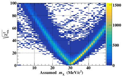
Figure 12: $\sqrt{\chi^{2}_{\mathrm{vtx}}}$ distribution for the MC signal events at $(m_{\mathrm{X}},\tau_{\mathrm{X}})=(30\leavevmode\nobreak\ \mathrm{MeV/c^{2}},20\leavevmode\nobreak\ \mathrm{ps})$ as a function of $m_{\mathrm{X}}$ assumed in the reconstruction.

Figure 12 shows the dependence of $\chi^{2}_{\mathrm{vtx}}$ on the assumed value of $m_{\mathrm{X}}$ for the MC signal events, providing another rationale for Eq. (14). When the assumed value is the same as the true value ($m_{\mathrm{X}}=30$ MeV/c² in this case), the resultant $\chi^{2}_{\mathrm{vtx}}$ becomes minimum on average. The effective $m_{\mathrm{X}}$ resolution is $\sim 2.5$ MeV/c².

5.3.2 Momentum

Given the vertex position, the momentum of each $\gammaup$ can be calculated. The sum of the final-state three particles momenta,

$$\mbox{\boldmath$P$}_{\mathrm{sum}}\equiv\mbox{\boldmath$P$}_{\mathrm{e^{+}}}+\mbox{\boldmath$P$}_{\gammaup_{1}}+\mbox{\boldmath$P$}_{\gammaup_{2}},$$ (15)

should be 0 for the MEx2G events.

5.3.3 Relative time

The time difference between the 2$\gammaup$s at the X vertex is calculated as

$$t_{\gammaup\gammaup}=\left(t_{\gammaup_{1}}-\frac{l_{\gammaup_{1}}}{c}\right)-\left(t_{\gammaup_{2}}-\frac{l_{\gammaup_{2}}}{c}\right),$$ (16)

where $l_{\gammaup_{1(2)}}$ is the distance between the $\gammaup_{1(2)}$ interaction point in the LXe photon detector and the X vertex position, $l_{\gammaup_{1(2)}}=|\mbox{\boldmath$x$}_{\gammaup_{1(2)}}-\mbox{\boldmath$x$}_{\mathrm{vtx}}|$. The relative position of the vertices is such that this definition is identical to the signed distance defined according to the X direction and therefore the distribution is centred at 0 for MEx2G events.

The time difference between $\gammaup_{1}$ and e⁺ at the muon vertex is calculated as

t_γ_1e^+$$=\left(t_{\gammaup_{1}}-\frac{l_{\gammaup_{1}}}{c}-\frac{l_{\mathrm{X}}}{\beta c}\right)-t_{\mathrm{e^{+}}}.$$ (17)

With the unsigned definition of $l_{\mathrm{X}}$ the distribution is slightly offset with respect to 0 for MEx2G events as visible in Fig. 14d.

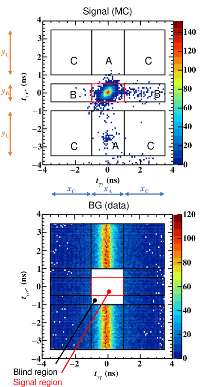
Figure 13: Top: Signal (MC) and bottom: background (sideband data) event distributions in the $t_{\gammaup_{1}\mathrm{e^{+}}}$–$t_{\gammaup\gammaup}$ plane before the signal selection criteria are applied. (20 MeV/c², 20 ps) case is shown as an example. The time sideband regions (A, B, C) and the signal region (the red box) are also shown.

6 Dataset and event selection

We use the full MEG dataset, collected in 2009–2013, as was used in the $\muup^{+}\to\mathrm{e}^{+}\gammaup$ search reported in baldini_2016 . As described in Sect. 2, the $\muup^{+}\to\mathrm{e}^{+}\gammaup$ trigger data are used in this analysis. In total, $7.5\times 10^{14}\,\muup^{+}$s were stopped on the target.

A pre-selection was applied at the first stage of the $\muup^{+}\to\mathrm{e}^{+}\gammaup$ decay analysis, requiring that at least one positron track is reconstructed and the time difference between signals in the LXe photon detector and TC is in the range $-6.9<t_{\mathrm{LXe}-\mathrm{TC}}<4.4\leavevmode\nobreak\ \mathrm{ns}$. At this stage, aiming to select the $\muup^{+}\to\mathrm{e}^{+}\gammaup$ decays, the time of the LXe photon detector is reconstructed with PMTs around the largest peak found in the peak search (Sect. 5.2.1). This retained $\sim$16% of the dataset, on which the full event reconstruction for the $\muup^{+}\to\mathrm{e}^{+}\gammaup$ decay analysis was performed. Before processing the MEx2G dedicated reconstruction, we applied an additional event selection using the $\muup^{+}\to\mathrm{e}^{+}\gammaup$ reconstruction results. It was based on the existence of multiple ($\geq\!2$) $\gammaup$s and the total energy of the $\gammaup$s and e⁺ ($E_{\mathrm{total}}$) being $|E_{\mathrm{total}}-m_{\muup}|<0.2m_{\muup}$. This selection reduces the dataset by an additional factor of $\sim$ 300. We applied the MEx2G dedicated reconstruction (Sect. 5.2.2, 5.2.3, and 5.3) to this selected dataset.

A blind region was defined containing the events satisfying the cuts $|t_{\gammaup_{1}\mathrm{e^{+}}}|<1\,\mathrm{ns}\land|t_{\gammaup\gammaup}|<1\,\mathrm{ns}$. This blind region is large enough to hide the signal. Those events were sent in a separated data-stream and were not used in the definition of the analysis strategy including cuts; background events in the signal region were estimated without using events in the blind region. After the analysis strategy was defined, the blind region was opened and events in this region were added to perform the last step of analysis.

The accidental background can be estimated from the off-time sideband regions defined in Fig. 13. There are three such regions: A, B, and C; each containing a different combination of the types of background as defined in Sect. 3. The outer boundary of the time sidebands, $|t_{\gammaup_{1}\mathrm{e^{+}}}|<3.5\,\mathrm{ns}\land|t_{\gammaup\gammaup}|<3.5\,\mathrm{ns}$, are determined so that the background distribution is not deformed by the time-coincidence trigger condition. The widths $x_{\mathrm{A}}$ and $y_{\mathrm{B}}$ in Fig. 13 are the same as the outer boundary of the signal region defined depending on $m_{X}$ by the signal selection criteria described below.

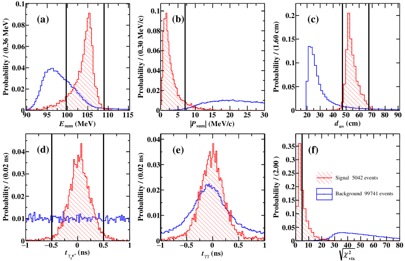
Figure 14: Distributions of variables used in the event selection for $(m_{\mathrm{X}},\tau_{\mathrm{X}})$ = (20 MeV/c², 20 ps) case. The hatched histograms show the distribution of MC signal events while the blank histograms that of background events; each histogram is normalised to 1. The vertical lines show the optimised thresholds. (a) The peak value of the signal distribution is at $m_{\muup}$ with FWHM${}_{E_{\mathrm{sum}}}$ = 2.7 MeV. (c) Cut-off at 20 cm in the background distribution comes from one of the 2$\gammaup$ reconstruction conditions. (e) The threshold lines are not visible because they are set to $\pm 1$ ns. For a detailed definition of the variables see Sect. 6.

The following seven variables are used for the signal selection:

1. $E_{\mathrm{e^{+}}}$: the e⁺ energy.

2. $E_{\mathrm{sum}}$: the total energy of the three particles.

3. $|\mbox{\boldmath$P$}_{\mathrm{sum}}|$: the magnitude of the sum of the three particles’ momenta.

4. $d_{uv}$: the distance between the 2$\gammaup$ positions on the LXe photon detector inner face.

5. $t_{\gammaup_{1}\mathrm{e^{+}}}$: the time difference between $\gammaup_{1}$ and e⁺ calculated in Eq. (17).

6. $t_{\gammaup\gammaup}$: the time difference between 2$\gammaup$s calculated in Eq. (16).

7. $\chi^{2}_{\mathrm{vtx}}$: the goodness of vertex fitting calculated in Eq. (14).

First, we fix the $E_{\mathrm{e^{+}}}$ selection to require $|E_{\mathrm{e^{+}}}-E_{\mathrm{e^{+}}}^{m_{\mathrm{X}}}|<1$ MeV, where $E_{\mathrm{e^{+}}}^{m_{\mathrm{X}}}$ is the e⁺ energy for the MEx2G decay with $m_{\mathrm{X}}$. This selection is also used in the Michel normalisation described in Sect. 7.

Next, we optimise the cut thresholds for the other variables to maximise the experimental outcomes. Distributions of these variables for the signal and background at a parameter set (20 MeV/c², 20 ps) are shown in Fig. 14. All other selection criteria, such as trigger and reconstruction conditions as well as the $E_{\mathrm{e^{+}}}$ selection, are applied. The time sideband events are used for the background distribution, while MC samples are used for the signal distribution.

Punzi’s expression Punzi2003 is used as a figure of merit

$$F_{\mathrm{Punzi}}=\frac{\epsilon_{\mathrm{selection}}}{b^{2}+2a\sqrt{N_{\mathrm{BG}}}+b\sqrt{b^{2}+4a\sqrt{N_{\mathrm{BG}}}+4N_{\mathrm{BG}}}},$$ (18)

where $a$ and $b$ are the significance and the power of a test, respectively, $\epsilon_{\mathrm{selection}}$ is the selection efficiency for the signal, and $N_{\mathrm{BG}}$ is the expected number of background events. The values of $a$ and $b$ should be defined before the analysis, and we set $a=3,b=1.28\,(=90\%)$, where $b$ is set to the value appropriate to the confidence level being used to set the upper limit when a non-significant result is obtained.

The optimisation process is divided into two steps. In the first step, we optimise the cut thresholds of variables 2–6, independently for each variable in order to maintain high statistics in the sidebands. Because the absolute value of $N_{\mathrm{BG}}$ does not make sense in this independent optimisation process, we approximate $N_{\mathrm{BG}}$ to $\epsilon_{\mathrm{BG}}$, a selection efficiency for the background events calculated using the time sideband samples selected up to this point. Because of this approximation, the first step leads to suboptimal criteria.

In the second step, after all other selection criteria are applied, the threshold for $\chi^{2}_{\mathrm{vtx}}$ is optimised to give the highest $F_{\mathrm{Punzi}}$. In this step, to estimate $N_{\mathrm{BG}}$ from the low statistics in the sideband regions, we use a kernel-density-estimation method Crabner2001 to model the continuous event distribution.

The cut thresholds are optimised at 5 $\mathrm{MeV/c^{2}}$ intervals in $m_{\mathrm{X}}$, while the same thresholds are used for different $\tau_{\mathrm{X}}$ for each $m_{\mathrm{X}}$. The optimised thresholds for $m_{\mathrm{X}}=20\leavevmode\nobreak\ \mathrm{MeV/c^{2}}$ are shown as black lines in Fig. 14. These cuts result in $\epsilon_{\mathrm{selection}}=67\%$ ($m_{\mathrm{X}}=45$ MeV/c²) – 51% ($m_{\mathrm{X}}=20$ MeV/c²).

7 Single event sensitivity

The single event sensitivity of the MEx2G decay $s$ is defined as follows:

$$\mathcal{B}_{\mathrm{MEx2G}}=s\times N_{\mathrm{MEx2G}},$$ (19)

where $N_{\mathrm{MEx2G}}$ is the expected number of signal events in the signal region. We calculate it using Michel decay ($\muup^{+}\to{\rm e}^{+}\nuup\bar{\nuup}$) events taken at the same time with the $\muup^{+}\to\mathrm{e}^{+}\gammaup$ trigger. This Michel normalisation is beneficial for the following reasons. First, systematic uncertainties coming from the muon beam are cancelled because beam instability is included in both Michel triggered and the $\muup^{+}\to\mathrm{e}^{+}\gammaup$ triggered events. Moreover, we do not need to know the $\muup^{+}$ stopping rate nor the live DAQ time. Second, most of the systematic uncertainties coming from e⁺ detection are also cancelled. The absolute value of e⁺ efficiency is not needed.

The number of Michel events is given by

$$N_{\mathrm{Michel}}=N_{\muup^{+}}\cdot\frac{\mathcal{B}_{\mathrm{Michel}}\cdot f_{\mathrm{Michel}}}{p_{\mathrm{Michel}}\cdot p_{\mathrm{correction}}}\cdot A_{\mathrm{Michel}}\cdot\epsilon_{\mathrm{Michel}},$$ (20)

where

$N_{\muup^{+}}$:

the number of stopped $\muup^{+}$s;

$\mathcal{B}_{\mathrm{Michel}}$:

branching ratio of the Michel decay ($\approx 1$);

$f_{\mathrm{Michel}}$:

branching fraction of the selected energy region (7%–10% depending on $m_{\mathrm{X}}$);

$p_{\mathrm{Michel}}$:

prescaling factor of the Michel trigger ($=10^{7}$);

$p_{\mathrm{correction}}$:

correction factor of $p_{\mathrm{Michel}}$ depending on the muon beam intensity;

$A_{\mathrm{Michel}}$:

geometrical acceptance of the spectrometer for Michel e⁺s;

$\epsilon_{\mathrm{Michel}}$:

e⁺ efficiency for Michel events within the geometrical acceptance of the spectrometer.

The number of MEx2G events is given by

$$N_{\mathrm{MEx2G}} = N_{\muup^{+}}\cdot\frac{\mathcal{B}_{\mathrm{MEx2G}}}{p_{\mathrm{MEG}}}\cdot A_{\mathrm{e^{+}}}\cdot\epsilon_{\mathrm{e^{+}}}\cdot\epsilon_{2\gammaup}\cdot\epsilon_{\mathrm{DM}}\cdot\epsilon_{\mathrm{selection}},$$ (21)

where

$p_{\mathrm{MEG}}$:

prescaling factor of the $\muup^{+}\to\mathrm{e}^{+}\gammaup$ trigger (=1);

$A_{\mathrm{e^{+}}}$:

geometrical acceptance of the spectrometer for MEx2G e⁺s;

$\epsilon_{\mathrm{e^{+}}}$:

e⁺ efficiency for MEx2G events conditional to e⁺s in the geometrical acceptance of the spectrometer;

$\epsilon_{2\gammaup}$:

the product of 2$\gammaup$ geometrical acceptance and 2$\gammaup$ trigger, detection, and reconstruction efficiency, conditional to the e⁺ detection;

$\epsilon_{\mathrm{DM}}$:

the trigger direction match efficiency conditional to the e⁺ and $2\gammaup$ detection (Fig. 6);

$\epsilon_{\mathrm{selection}}$:

the signal selection efficiency.

Using Eqs. (19)–(21), an estimate of the SES ($s_{0}$) is given by

$$s_{0}^{-1} = N_{\mathrm{Michel}}\frac{1}{\mathcal{B}_{\mathrm{Michel}}\cdot f_{\mathrm{Michel}}}\cdot\frac{p_{\mathrm{Michel}}\cdot p_{\mathrm{correction}}}{p_{\mathrm{MEG}}}$$ (22)

$$\cdot\frac{A_{\mathrm{e^{+}}}}{A_{\mathrm{Michel}}}\cdot\frac{\epsilon_{\mathrm{e^{+}}}}{\epsilon_{\mathrm{Michel}}}\cdot\epsilon_{2\gammaup}\cdot\epsilon_{\mathrm{DM}}\cdot\epsilon_{\mathrm{selection}}.$$

The geometrical acceptance of the spectrometer is common, hence $A_{\mathrm{e^{+}}}/A_{\mathrm{Michel}}=1$; the estimate of the relative e⁺ efficiency is $\epsilon_{\mathrm{e^{+}}}/\epsilon_{\mathrm{Michel}}=89\%\ (m_{\mathrm{X}}=45$ MeV/c${}^{2})\ -\ 97\%\ (m_{\mathrm{X}}=20$ MeV/c${}^{2})$ increasing monotonically with $m_{\mathrm{X}}$. The estimate of $\epsilon_{2\gammaup}$ is shown in Fig. 15; $\epsilon_{2\gammaup}=0.6\%$ ($m_{\mathrm{X}}=45$ MeV/c²) – 2.9% ($m_{\mathrm{X}}=20$ MeV/c²), decreasing monotonically with $m_{\mathrm{X}}$. This dependence comes mainly from the 2$\gammaup$ acceptance: for increasing $m_{\mathrm{X}}$, the opening angle between the 2$\gammaup$s becomes larger, resulting in a decreasing efficiency.

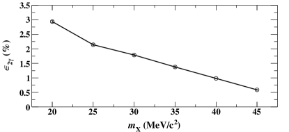
Figure 15: $\epsilon_{2\gammaup}$ (see the text for the definition) versus $m_{\mathrm{X}}$ for $\tau_{\mathrm{X}}=20$ ps.

The systematic uncertainties are summarised in Table 1. The uncertainty in the 2$\gammaup$ detection efficiency and that in the MC smearing parameters are the dominant components.

Table 1: Systematic uncertainties in the single event sensitivity ($\tau_{\mathrm{X}}=20$ ps).

$m_{\mathrm{X}}$ (MeV/c2)	20	25	30	35	40	45
Michel e+ counting	0.99%	1.1%	1.1%	0.93%	1.6%	2.8%
Relative e+ efficiency	1.4%	0.18%	0.31%	0.55%	0.89%	1.3%
2$\gammaup$ acceptance	1.3%	2.0%	3.4%	2.9%	5.4%	1.9%
$\gammaup$ trigger efficiency	0.98%	0.32%	0.26%	0.52%	1.4%	3.2%
2$\gammaup$ detection efficiency	7.9%	7.9%	7.9%	7.9%	7.9%	7.9%
MC statistics	1.8%	1.9%	2.2%	3.1%	1.9%	4.7%
MC smearing	4.8%	3.4%	3.8%	5.3%	3.3%	14%
Total	9.7%	9.1%	9.7%	11%	10%	17%

The estimated value of SES is $s_{0}=(2.9\pm 0.3)\times 10^{-12}$ (20 MeV/c²) – $(6.3\pm 1.1)\times 10^{-10}$ (45 MeV/c²) for $\tau_{\mathrm{X}}=20$ ps increasing monotonically with $m_{\mathrm{X}}$. The e⁺ efficiency is $\epsilon_{\mathrm{e^{+}}}=1\%$ (45 MeV/c²) – 36% (20 MeV/c²) decreasing monotonically with $m_{\mathrm{X}}$, estimated with the MC, although this quantity is not necessary for the normalisation. The overall efficiency for the MEx2G events conditional to the e⁺ in the geometrical acceptance of the spectrometer is therefore $\epsilon_{\mathrm{MEx2G}}=2.0\times 10^{-5}$ (45 MeV/c²) – $4.7\times 10^{-3}$ (20 MeV/c²) decreasing monotonically with $m_{\mathrm{X}}$.

8 Statistical treatment of background and signal

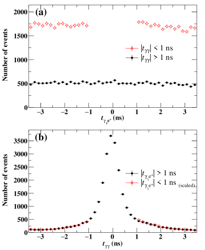
Figure 16: Time distributions in the sideband regions for (20 MeV/c², 20 ps). (a) $t_{\gammaup_{1}\mathrm{e^{+}}}$ distributions for $|t_{\gammaup\gammaup}|<1$ ns (red open circles) and for $1<|t_{\gammaup\gammaup}|<3.5$ ns (black closed circles). (b) $t_{\gammaup\gammaup}$ distributions for $|t_{\gammaup_{1}\mathrm{e^{+}}}|<1$ ns (red open circles) and for $1<|t_{\gammaup_{1}\mathrm{e^{+}}}|<3.5$ ns scaled by the ratio of the time ranges (black closed circles). A loose cut is applied: $|E_{\mathrm{e^{+}}}-E_{\mathrm{e^{+}}}^{m_{\mathrm{X}}}|<1\leavevmode\nobreak\ \mathrm{MeV}\land E_{\mathrm{sum}}<115\leavevmode\nobreak\ \mathrm{MeV}\land|\mbox{\boldmath$P$}_{\mathrm{sum}}|<30\leavevmode\nobreak\ \mathrm{MeV/c}\land d_{uv}<90\leavevmode\nobreak\ \mathrm{cm}\land\chi^{2}_{\mathrm{vtx}}<80$.

In the following, we describe how we estimate the expected number of background events in the signal region ($N_{\mathrm{BG}}$) from the numbers of events observed in sidebands A, B, and C ($N_{\mathrm{A}}^{\mathrm{obs}}$, $N_{\mathrm{B}}^{\mathrm{obs}}$, and $N_{\mathrm{C}}^{\mathrm{obs}}$).

There are three types of accidental background events defined in Sect. 3. The expected number of background events in the signal region is given by

$$N_{\mathrm{BG}}=N_{1}+N_{2}+N_{3},$$ (23)

where $N_{1},N_{2},N_{3}$ are the expected numbers of background events in the signal region from the types 1, 2, and 3, respectively. Sideband A has the contributions from types 2 and 3, B has the contributions from types 1 and 3, and C has the contribution from type 3.

Figure 16 shows the time distributions in the sideband regions. A peak of type 2 on a flat component of type 3 is observed in the $t_{\gammaup\gammaup}$ distribution, while a peak of type 1 is not clearly visible in the $t_{\gammaup_{1}\mathrm{e^{+}}}$ distribution. The uniformity of the accidental backgrounds is examined using these distributions; the number of events in ($|t_{\gammaup_{1}\mathrm{e^{+}}}|<1\leavevmode\nobreak\ \mathrm{ns}\land 1<|t_{\gammaup\gammaup}|<3.5\leavevmode\nobreak\ \mathrm{ns}$) is compared to the the number of events interpolated from the region ($1<|t_{\gammaup_{1}\mathrm{e^{+}}}|<3.5\leavevmode\nobreak\ \mathrm{ns}\land 1<|t_{\gammaup\gammaup}|<3.5\leavevmode\nobreak\ \mathrm{ns}$) scaled by the ratio of the widths of the time ranges (2 ns/5 ns). They agree within 1.7% (the central part, including type 1, is 1.7% larger than the interpolation). In Fig. 16b, $t_{\gammaup\gammaup}$ the distribution for $1<|t_{\gammaup_{1}\mathrm{e^{+}}}|<3.5$ ns is superimposed on that for $|t_{\gammaup_{1}\mathrm{e^{+}}}|<1$ ns after scaling by the time range ratio. The tail component of type 2 is consistent in these regions. The errors on the background estimations by the interpolation are thus negligibly small compared with the statistical uncertainties in $N_{\mathrm{A}}^{\mathrm{obs}},N_{\mathrm{B}}^{\mathrm{obs}},N_{\mathrm{C}}^{\mathrm{obs}}$.

Using $N_{1},N_{2},N_{3}$, the expected numbers of events in sidebands A, B, C can be calculated as follows:

$$N_{\mathrm{A}}^{\mathrm{exp}} = N_{2}\times\frac{2y_{\mathrm{C}}}{y_{\mathrm{B}}}+N_{3}\times\frac{2y_{\mathrm{C}}}{y_{\mathrm{B}}},$$ (24)

$$N_{\mathrm{B}}^{\mathrm{exp}} = N_{1}\times\frac{2x_{\mathrm{C}}}{x_{\mathrm{A}}}+N_{3}\times\frac{2x_{\mathrm{C}}}{x_{\mathrm{A}}}+N_{2}\times f_{\mathrm{escape}},$$ (25)

$$N_{\mathrm{C}}^{\mathrm{exp}} = N_{3}\times\frac{2y_{\mathrm{C}}}{y_{\mathrm{B}}}\times\frac{2x_{\mathrm{C}}}{x_{\mathrm{A}}}+N_{2}\times f_{\mathrm{escape}}\times\frac{2y_{\mathrm{C}}}{y_{\mathrm{B}}},$$ (26)

where $x_{\mathrm{A(C)}}$ and $y_{\mathrm{B(C)}}$ are the sizes of the signal regions (sideband regions) in $t_{\gammaup\gammaup}$ and $t_{\gammaup_{1}\mathrm{e^{+}}}$, respectively, as defined in Fig. 13, and $f_{\mathrm{escape}}=0.171\pm 0.003$ is the fraction of type 2 events in $|t_{\gammaup\gammaup}|>1\,\mathrm{ns}$.

The likelihood function for $N_{\mathrm{BG}}$ is given from the Poisson statistics as,

$$\mathcal{L} (N_{\mathrm{BG}}\mid N_{\mathrm{A}}^{\mathrm{obs}},N_{\mathrm{B}}^{\mathrm{obs}},N_{\mathrm{C}}^{\mathrm{obs}})$$ (27)

$$= P_{\mathrm{Poi}}(N_{\mathrm{A}}^{\mathrm{obs}}\mid N_{\mathrm{A}}^{\mathrm{exp}})P_{\mathrm{Poi}}(N_{\mathrm{B}}^{\mathrm{obs}}\mid N_{\mathrm{B}}^{\mathrm{exp}})P_{\mathrm{Poi}}(N_{\mathrm{C}}^{\mathrm{obs}}\mid N_{\mathrm{C}}^{\mathrm{exp}}).$$

The best estimate of $N_{\mathrm{BG}}$ can be obtained by maximising Eq. (27) (listed in Table 2). However, we do not use this estimated $N_{\mathrm{BG}}$ in the inference of the signal but use $(N_{\mathrm{A}}^{\mathrm{obs}},N_{\mathrm{B}}^{\mathrm{obs}},N_{\mathrm{C}}^{\mathrm{obs}})$ as discussed in the following.

Our goal is to estimate the branching ratio of the MEx2G decay ($\mathcal{B}_{\mathrm{MEx2G}}$). The likelihood function Eq. (27) is extended to include $\mathcal{B}_{\mathrm{MEx2G}}$ as a parameter and the number of events in the signal region ($N_{\mathrm{S}}^{\mathrm{obs}}$) as an observable. In addition, to incorporate the uncertainty in the SES into the $\mathcal{B}_{\mathrm{MEx2G}}$ estimation, the estimated SES ($s_{0}$) and the true value ($s$) are included into the likelihood function:

$$\mathcal{L}(\mathcal{B}_{\mathrm{MEx2G}},N_{\mathrm{BG}},s\mid N_{\mathrm{S}}^{\mathrm{obs}},N_{\mathrm{A}}^{\mathrm{obs}},N_{\mathrm{B}}^{\mathrm{obs}},N_{\mathrm{C}}^{\mathrm{obs}},s_{0}).$$ (28)

Using $N_{1},N_{2},N_{3}$ and a Gaussian PDF for the inverse of SES, it can be written as,

$$\mathcal{L} (\mathrm{\mathcal{B}_{\mathrm{MEx2G}}},N_{1},N_{2},N_{3},s\mid N_{\mathrm{S}}^{\mathrm{obs}},N_{\mathrm{A}}^{\mathrm{obs}},N_{\mathrm{B}}^{\mathrm{obs}},N_{\mathrm{C}}^{\mathrm{obs}},s_{0})$$ (29)

$$= P_{\mathrm{Poi}}(N_{\mathrm{S}}^{\mathrm{obs}}\mid N^{\mathrm{exp}}_{\mathrm{S}})P_{\mathrm{Poi}}(N_{\mathrm{A}}^{\mathrm{obs}}\mid N_{\mathrm{A}}^{\mathrm{exp}})P_{\mathrm{Poi}}(N_{\mathrm{B}}^{\mathrm{obs}}\mid N_{\mathrm{B}}^{\mathrm{exp}})$$

$$\times P_{\mathrm{Poi}}(N_{\mathrm{C}}^{\mathrm{obs}}\mid N_{\mathrm{C}}^{\mathrm{exp}})P_{\mathrm{Gaus}}(s_{0}^{-1}\mid s^{-1}),$$

where $N^{\mathrm{exp}}_{\mathrm{S}}=N_{1}+N_{2}+N_{3}+\mathcal{B}_{\mathrm{MEx2G}}/s$ is the expected number of events in the signal region.

The best estimated values of the parameter set $\{\mathcal{B}_{\mathrm{MEx2G}}$, $N_{1}$, $N_{2}$, $N_{3}$, $s\}$ are obtained by maximising Eq. (29). Among them, only $\mathcal{B}_{\mathrm{MEx2G}}$ is the interesting parameter, while the others are regarded as nuisance parameters $\mbox{\boldmath$\nu$}=(N_{1},N_{2},N_{3},s)$.

A frequentist test of the null (background-only) hypothesis is performed with the following profile likelihood ratio $\lambda_{p}$ as the test statistic PDG2018 :

$$\lambda_{p}(\mathcal{B}_{\mathrm{MEx2G}})=\frac{\mathcal{L}(\mathcal{B}_{\mathrm{MEx2G}},\hat{\hat{\mbox{\boldmath$\nu$}}})}{\mathcal{L}(\hat{\mathcal{B}}_{\mathrm{MEx2G}},\hat{\mbox{\boldmath$\nu$}})},$$ (30)

where $\hat{\mathcal{B}}_{\mathrm{MEx2G}}$ and $\hat{\mbox{\boldmath$\nu$}}$ are the best-estimated values, and $\hat{\hat{\mbox{\boldmath$\nu$}}}$ is the value of $\nu$ that maximises the likelihood at the fixed $\mathcal{B}_{\mathrm{MEx2G}}$. The systematic uncertainties of the background estimation and the SES are incorporated into the test by profiling the likelihood about $\nu$. The local significance is quantified by the p-value $p_{\mathrm{local}}$, defined as the probability to find $\lambda_{p}$ that is equally or less compatible with the null hypothesis than that observed with the data when the signal does not exist.

Since $m_{\mathrm{X}}$ is unknown, we need to take the look-elsewhere effect PDG2018 into account to calculate the global significance. We estimate this effect following the approaches in Gross2010 ; Davies1987 , in which the trial factor of the search is estimated using an asymptotic property of $\lambda_{p}$, obeying the chi-square distribution. The smallest $p_{\mathrm{local}}$ in the $m_{\mathrm{X}}$ scan is converted into the global p-value $p_{\mathrm{global}}$ assuming that the signal can appear only at one $m_{\mathrm{X}}$.

The range of $\mathcal{B}_{\mathrm{MEx2G}}$ at 90% C.L. is constructed based on the Feldman–Cousins unified approach Cousins1998 extended to use the profile-likelihood ratio as the ordering statistic in order to incorporate the systematic uncertainties Cranmer2005 .

Table 2: The number of observed events in the sideband regions and the signal region and the expected number of background events in the signal region.

$m_{\mathrm{X}}$ (MeV/c2)	$N_{\mathrm{A}}^{\mathrm{obs}}$	$N_{\mathrm{B}}^{\mathrm{obs}}$	$N_{\mathrm{C}}^{\mathrm{obs}}$	$N_{\mathrm{BG}}$	$N_{\mathrm{S}}^{\mathrm{obs}}$
20	0	0	1	$0.048_{-0.046}^{+0.202}$	1
21	0	0	3	$0.146_{-0.084}^{+0.198}$	0
22	1	0	5	$0.292_{-0.140}^{+0.211}$	0
23	3	0	3	$0.622_{-0.330}^{+0.425}$	0
24	2	0	1	$0.414_{-0.260}^{+0.346}$	1
25	2	0	3	$0.414_{-0.261}^{+0.346}$	0
26	0	0	3	$0.150_{-0.091}^{+0.189}$	0
27	0	0	1	$0.050_{-0.049}^{+0.200}$	0
28	0	0	1	$0.048_{-0.046}^{+0.202}$	0
29	0	0	1	$0.048_{-0.046}^{+0.202}$	1
30	0	0	0	$0.000_{-0.000}^{+0.170}$	0
31	0	0	1	$0.048_{-0.046}^{+0.202}$	0
32	0	0	0	$0.000_{-0.000}^{+0.170}$	0
33	0	0	0	$0.000_{-0.000}^{+0.210}$	0
34	0	0	0	$0.000_{-0.000}^{+0.210}$	1
35	0	0	0	$0.000_{-0.000}^{+0.210}$	2
36	0	0	0	$0.000_{-0.000}^{+0.210}$	2
37	1	0	0	$0.400_{-0.301}^{+0.517}$	1
38	0	0	2	$0.168_{-0.105}^{+0.183}$	0
39	0	0	1	$0.084_{-0.084}^{+0.201}$	0
40	0	0	0	$0.000_{-0.000}^{+0.210}$	0
41	0	0	0	$0.000_{-0.000}^{+0.210}$	0
42	0	0	0	$0.000_{-0.000}^{+0.210}$	0
43	0	0	1	$0.084_{-0.084}^{+0.201}$	0
44	0	0	0	$0.000_{-0.000}^{+0.210}$	0
45	0	0	0	$0.000_{-0.000}^{+0.210}$	0

9 Results and discussion

Table 2 summarises the numbers of events in the signal region and the sidebands as well as the expected number of background events in the signal region. We observe non-zero events in the signal region for some masses. Note that the adjacent $m_{\mathrm{X}}$ bins are not statistically independent. Summing up the observed events gives nine events but five of them are unique events. One event appears in four bins ($m_{\mathrm{X}}=$ 34, 35, 36, 37 MeV/c²) and another event appears in two bins ($m_{\mathrm{X}}=$ 35, 36 MeV/c²).

We discuss the results for $\tau_{\mathrm{X}}=20$ ps below. The results for other $\tau_{\mathrm{X}}$ are similar, with small changes in the efficiency. The results are presented in detail in Appendix A.

Figure 17 shows 90% confidence intervals on $\mathcal{B}_{\mathrm{MEx2G}}$ obtained from this analysis together with the sensitivities and the previous upper limits due to Crystal Box. The sensitivities are evaluated by the mean of the branching ratio limits at 90% C.L. under the null hypothesis. Note that since we adopt the Feldman–Cousins unified approach, a one-sided or two-sided interval is automatically determined according to the data. Therefore, lower limits can be set in $m_{\mathrm{X}}$ regions where non-zero events are observed with small $N_{\mathrm{BG}}$.

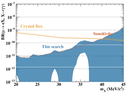
Figure 17: Confidence intervals (90% C.L.) on $\mathcal{B}_{\mathrm{MEx2G}}$ (blue band) for $\tau_{\mathrm{X}}=20$ ps. The red broken line shows the expected upper limits under the null hypothesis and the yellow line shows the limits extracted by Crystal Box analysis.

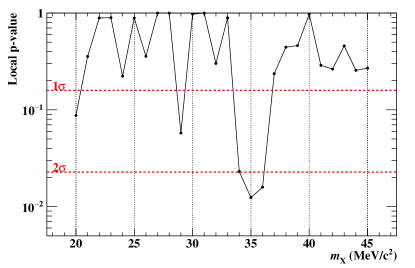
Figure 18: Local p-value under null hypothesis as a function of assumed $m_{\mathrm{X}}$.

The statistical significance of the excesses is tested against the null hypothesis. Figure 18 shows $p_{\mathrm{local}}$ versus $m_{\mathrm{X}}$. We observe the lowest $p_{\mathrm{local}}=0.012$ at $m_{\mathrm{X}}=35$ MeV/c², which corresponds to 2.2$\sigma$ significance. The global p-value is calculated to be $p_{\mathrm{global}}\approx 0.10$ by taking the look-elsewhere effect into account. This corresponds to 1.3$\sigma$, that is not statistically significant.

Owing to the large statistics of the MEG dataset, the branching ratio upper limits have been reduced to the level of $\mathcal{O}(10^{-11})$. Our results improves the upper limits from the Crystal Box experiment for $m_{\mathrm{X}}<40\,\mathrm{MeV/c^{2}}$, by a factor of 60 at most.

This publication reports results from the full MEG dataset. Hence, new experiments will be needed for further exploration of this decay, e.g. to test whether the small excess observed in this search grows. An upgraded experiment, MEG II, is currently being prepared baldini_2018 . A brief prospect for improved sensitivity to MEx2G in MEG II is discussed below. In this analysis the sensitivity worsens with increasing $m_{\mathrm{X}}$, mainly due to the 2$\gammaup$ acceptance and direction match efficiencies. The acceptance is determined by the geometry of the LXe photon detector and is not changed by the upgrade. The direction match efficiency can even worsen if we only consider the $\muup^{+}\to\mathrm{e}^{+}\gammaup$ search; the $\gammaup$ position resolution is expected to improve by a factor two, which enables tightening the direction match trigger condition. However, the MEG II trigger development is underway and the trigger efficiency for high mass can be improved up to a factor $\sim 2$ if a dedicated trigger is prepared. Basically, MEG II will collect ten times more $\muup^{+}$ decays and the resolutions of each kinematic variable will improve by roughly a factor two, leading to higher efficiency while maintaining low background. It is therefore possible to improve the sensitivity by one order of magnitude.

10 Conclusions

We have searched for a lepton-flavour-violating muon decay mediated by a new light particle, $\muup^{+}\to\mathrm{e}^{+}\mathrm{X},\mathrm{X}\to\gammaup\gammaup$ decay, for the first time using the full dataset (2009–2013) of the MEG experiment. No significant excess was found in the mass range $m_{\mathrm{X}}=20$–45 MeV/c² and $\tau_{\mathrm{X}}<40$ ps, and we set new branching ratio upper limits in the mass range $m_{\mathrm{X}}=20$–40 MeV/c². In particular, the upper limits are lowered to the level of $\mathcal{O}(10^{-11})$ for $m_{\mathrm{X}}=20$–30 MeV/c². The result is up to 60 times more stringent than the bound converted from the previous experiment, Crystal Box.

Appendix A Detailed results for different lifetimes

The detailed results for different lifetimes $\tau_{\mathrm{X}}$ are summarised in Tables 3–5.

Table 3: Results for $\tau_{\mathrm{X}}=5$ ps. LL and UL denote the lower limit and upper limit of the 90% confidence interval.

$m_{\mathrm{X}}$ (MeV/c2)	$s_{0}$	LL	UL
20	$(3.29\pm 0.31)\times 10^{-12}$	$4.60\times 10^{-13}$	$1.28\times 10^{-11}$
21	$(3.56\pm 0.44)\times 10^{-12}$	–	$7.78\times 10^{-12}$
22	$(3.73\pm 0.44)\times 10^{-12}$	–	$8.30\times 10^{-12}$
23	$(3.96\pm 0.45)\times 10^{-12}$	–	$7.72\times 10^{-12}$
24	$(4.26\pm 0.49)\times 10^{-12}$	–	$1.43\times 10^{-11}$
25	$(5.41\pm 0.55)\times 10^{-12}$	–	$1.08\times 10^{-11}$
26	$(5.16\pm 0.61)\times 10^{-12}$	–	$1.13\times 10^{-11}$
27	$(5.81\pm 0.70)\times 10^{-12}$	–	$1.39\times 10^{-11}$
28	$(6.62\pm 0.81)\times 10^{-12}$	–	$1.58\times 10^{-11}$
29	$(7.67\pm 0.95)\times 10^{-12}$	$8.53\times 10^{-13}$	$2.93\times 10^{-11}$
30	$(8.62\pm 0.85)\times 10^{-12}$	–	$2.26\times 10^{-11}$
31	$(1.07\pm 0.14)\times 10^{-11}$	–	$2.54\times 10^{-11}$
32	$(1.29\pm 0.17)\times 10^{-11}$	–	$3.20\times 10^{-11}$
33	$(1.59\pm 0.21)\times 10^{-11}$	–	$4.00\times 10^{-11}$
34	$(1.97\pm 0.26)\times 10^{-11}$	$1.97\times 10^{-12}$	$7.66\times 10^{-11}$
35	$(2.60\pm 0.31)\times 10^{-11}$	$1.65\times 10^{-11}$	$1.40\times 10^{-10}$
36	$(3.18\pm 0.42)\times 10^{-11}$	$1.98\times 10^{-11}$	$1.72\times 10^{-10}$
37	$(4.12\pm 0.53)\times 10^{-11}$	–	$1.43\times 10^{-10}$
38	$(5.43\pm 0.70)\times 10^{-11}$	–	$1.27\times 10^{-10}$
39	$(7.25\pm 0.93)\times 10^{-11}$	–	$1.79\times 10^{-10}$
40	$(9.01\pm 0.93)\times 10^{-11}$	–	$2.20\times 10^{-10}$
41	$(1.35\pm 0.19)\times 10^{-10}$	–	$3.37\times 10^{-10}$
42	$(1.88\pm 0.27)\times 10^{-10}$	–	$4.72\times 10^{-10}$
43	$(2.66\pm 0.39)\times 10^{-10}$	–	$6.47\times 10^{-10}$
44	$(3.81\pm 0.57)\times 10^{-10}$	–	$1.01\times 10^{-9}$
45	$(6.25\pm 0.88)\times 10^{-10}$	–	$1.59\times 10^{-9}$

Table 4: Results for $\tau_{\mathrm{X}}=20$ ps. LL and UL denote the lower limit and upper limit of the 90% confidence interval.

$m_{\mathrm{X}}$ (MeV/c2)	$s_{0}$	LL	UL
20	$(2.92\pm 0.28)\times 10^{-12}$	$3.94\times 10^{-13}$	$1.10\times 10^{-11}$
21	$(3.18\pm 0.39)\times 10^{-12}$	–	$7.54\times 10^{-12}$
22	$(3.35\pm 0.39)\times 10^{-12}$	–	$7.36\times 10^{-12}$
23	$(3.57\pm 0.40)\times 10^{-12}$	–	$7.14\times 10^{-12}$
24	$(3.86\pm 0.43)\times 10^{-12}$	–	$1.33\times 10^{-11}$
25	$(4.74\pm 0.43)\times 10^{-12}$	–	$1.06\times 10^{-11}$
26	$(4.71\pm 0.53)\times 10^{-12}$	–	$1.15\times 10^{-11}$
27	$(5.31\pm 0.62)\times 10^{-12}$	–	$1.33\times 10^{-11}$
28	$(6.07\pm 0.72)\times 10^{-12}$	–	$1.58\times 10^{-11}$
29	$(7.04\pm 0.85)\times 10^{-12}$	$1.04\times 10^{-12}$	$2.70\times 10^{-11}$
30	$(7.94\pm 0.78)\times 10^{-12}$	–	$2.07\times 10^{-11}$
31	$(9.86\pm 1.26)\times 10^{-12}$	–	$2.33\times 10^{-11}$
32	$(1.19\pm 0.15)\times 10^{-11}$	–	$3.14\times 10^{-11}$
33	$(1.46\pm 0.19)\times 10^{-11}$	–	$3.92\times 10^{-11}$
34	$(1.82\pm 0.23)\times 10^{-11}$	$2.25\times 10^{-12}$	$7.10\times 10^{-11}$
35	$(2.38\pm 0.25)\times 10^{-11}$	$1.53\times 10^{-11}$	$1.31\times 10^{-10}$
36	$(2.93\pm 0.37)\times 10^{-11}$	$1.85\times 10^{-11}$	$1.56\times 10^{-10}$
37	$(3.79\pm 0.47)\times 10^{-11}$	–	$1.29\times 10^{-10}$
38	$(4.99\pm 0.62)\times 10^{-11}$	–	$1.16\times 10^{-10}$
39	$(6.65\pm 0.83)\times 10^{-11}$	–	$1.66\times 10^{-10}$
40	$(8.20\pm 0.87)\times 10^{-11}$	–	$2.04\times 10^{-10}$
41	$(1.23\pm 0.20)\times 10^{-10}$	–	$3.15\times 10^{-10}$
42	$(1.71\pm 0.28)\times 10^{-10}$	–	$4.44\times 10^{-10}$
43	$(2.41\pm 0.41)\times 10^{-10}$	–	$5.98\times 10^{-10}$
44	$(3.44\pm 0.61)\times 10^{-10}$	–	$8.25\times 10^{-10}$
45	$(6.29\pm 1.12)\times 10^{-10}$	–	$1.63\times 10^{-9}$

Table 5: Results for $\tau_{\mathrm{X}}=40$ ps. LL and UL denote the lower limit and upper limit of the 90% confidence interval.

$m_{\mathrm{X}}$ (MeV/c2)	$s_{0}$	LL	UL
20	$(3.02\pm 0.29)\times 10^{-12}$	$3.78\times 10^{-13}$	$1.19\times 10^{-11}$
21	$(3.28\pm 0.39)\times 10^{-12}$	–	$7.44\times 10^{-12}$
22	$(3.44\pm 0.39)\times 10^{-12}$	–	$7.80\times 10^{-12}$
23	$(3.66\pm 0.40)\times 10^{-12}$	–	$7.41\times 10^{-12}$
24	$(3.94\pm 0.43)\times 10^{-12}$	–	$1.43\times 10^{-11}$
25	$(4.83\pm 0.43)\times 10^{-12}$	–	$1.04\times 10^{-11}$
26	$(4.76\pm 0.54)\times 10^{-12}$	–	$1.09\times 10^{-11}$
27	$(5.35\pm 0.61)\times 10^{-12}$	–	$1.33\times 10^{-11}$
28	$(6.09\pm 0.71)\times 10^{-12}$	–	$1.51\times 10^{-11}$
29	$(7.03\pm 0.83)\times 10^{-12}$	$9.22\times 10^{-13}$	$2.71\times 10^{-11}$
30	$(7.87\pm 0.78)\times 10^{-12}$	–	$1.88\times 10^{-11}$
31	$(9.78\pm 1.21)\times 10^{-12}$	–	$2.33\times 10^{-11}$
32	$(1.18\pm 0.15)\times 10^{-11}$	–	$2.92\times 10^{-11}$
33	$(1.44\pm 0.18)\times 10^{-11}$	–	$3.57\times 10^{-11}$
34	$(1.78\pm 0.22)\times 10^{-11}$	$1.97\times 10^{-12}$	$6.81\times 10^{-11}$
35	$(2.30\pm 0.23)\times 10^{-11}$	$1.47\times 10^{-11}$	$1.26\times 10^{-10}$
36	$(2.84\pm 0.34)\times 10^{-11}$	$1.78\times 10^{-11}$	$1.54\times 10^{-10}$
37	$(3.67\pm 0.43)\times 10^{-11}$	–	$1.28\times 10^{-10}$
38	$(4.80\pm 0.56)\times 10^{-11}$	–	$1.12\times 10^{-10}$
39	$(6.37\pm 0.75)\times 10^{-11}$	–	$1.51\times 10^{-10}$
40	$(7.94\pm 0.78)\times 10^{-11}$	–	$1.90\times 10^{-10}$
41	$(1.17\pm 0.18)\times 10^{-10}$	–	$2.84\times 10^{-10}$
42	$(1.62\pm 0.25)\times 10^{-10}$	–	$4.28\times 10^{-10}$
43	$(2.27\pm 0.37)\times 10^{-10}$	–	$5.94\times 10^{-10}$
44	$(3.23\pm 0.54)\times 10^{-10}$	–	$8.31\times 10^{-10}$
45	$(5.65\pm 0.97)\times 10^{-10}$	–	$1.53\times 10^{-9}$

References

- (1) Y. Fukuda et al. (Super-Kamiokande Collaboration), Evidence for oscillation of atmospheric neutrinos. Phys. Rev. Lett. 81(8), 1562 (1998). doi:10.1103/PhysRevLett.81.1562, arXiv:9807003
- (2) Q. R. Ahmad et al. (SNO Collaboration), Direct evidence for neutrino flavor transformation from neutral-current interactions in the Sudbury Neutrino Observatory. Phys. Rev. Lett. 89(1), 011301 (2002). doi:10.1103/PhysRevLett.89.011301, arXiv:nucl-ex/0204008
- (3) M. Tanabashi et al. (Particle Data Group), Review of Particle Physics. Phys. Rev. D 98(3) (2018). doi:10.1103/PhysRevD.98.030001
- (4) S. T. Petcov, The processes , , in the Weinberg-Salam model with neutrino mixing. Sov. J. Nucl. Phys. 25, 340 (1977). Erratum ibid. 25 (1977) 698
- (5) T. P. Cheng, L.-F. Li, in theories with Dirac and Majorana neutrino-mass terms. Phys. Rev. Lett. 45(24), 1908–1911 (1980). doi:10.1103/PhysRevLett.45.1908
- (6) R. Barbieri, L. J. Hall, Signals for supersymmetric unification. Phys. Lett. B 338(2–3), 212–218 (1994). doi:10.1016/0370-2693(94)91368-4, arXiv:hep-ph/9408406
- (7) T. Mori, W. Ootani, Flavour violating muon decays. Prog. Part. Nucl. Phys. 79, 57–94 (2014). doi:10.1016/j.ppnp.2014.09.001
- (8) L. Calibbi, G. Signorelli, Charged lepton flavour violation: An experimental and theoretical introduction. Riv. Nuovo Cim. 41(2), 71–174 (2018). doi:10.1393/ncr/i2018-10144-0
- (9) A. M. Baldini et al. (MEG Collaboration), Search for the lepton flavour violating decay with the full dataset of the MEG experiment. Eur. Phys. J. C 76(8), 434 (2016). doi:10.1140/epjc/s10052-016-4271-x
- (10) R. D. Peccei, H. R. Quinn, CP conservation in the presence of pseudoparticles. Phys. Rev. Lett. 38(25), 1440–1443 (1977). doi:10.1103/PhysRevLett.38.1440
- (11) S. Weinberg, A new light boson? Phys. Rev. Lett. 40(4), 223–226 (1978). doi:10.1103/PhysRevLett.40.223
- (12) F. Wilczek, Problem of strong P and T invariance in the presence of instantons. Phys. Rev. Lett. 40(5), 279–282 (1978). doi:10.1103/PhysRevLett.40.279
- (13) C. Cornella, P. Paradisi, O. Sumensari, Hunting for ALPs with lepton flavor violation. J. High Energy Phys. 158 (2020). arXiv:1911.06279v1
- (14) Y. Chikashige, R. N. Mohapatra, R. D. Peccei, Are there real goldstone bosons associated with broken lepton number? Phys. Lett. B 98(4), 265–268 (1981). doi:10.1016/0370-2693(81)90011-3
- (15) G. B. Gelmini, M. Roncadelli, Left-handed neutrino mass scale and spontaneously broken lepton number. Phys. Lett. B 99(5), 411–415 (1981). doi:10.1016/0370-2693(81)90559-1
- (16) D. B. Reiss, Can the family group be a global symmetry? Phys. Lett. B 115(3), 217–220 (1982). doi:10.1016/0370-2693(82)90647-5
- (17) F. Wilczek, Axions and family symmetry breaking. Phys. Rev. Lett. 49(21), 1549–1552 (1982). doi:10.1103/PhysRevLett.49.1549
- (18) Z. Berezhiani, M. Khlopov, Physical and astrophysical consequences of breaking of the symmetry of families. (In Russian). Sov. J. Nucl. Phys. 51, 1479–1491 (1990)
- (19) J. Jaeckel, A family of WISPy dark matter candidates. Phys. Lett. B 732, 1–7 (2014). doi:10.1016/j.physletb.2014.03.005, arXiv:1311.0880
- (20) K. Tsumura, L. Velasco-Sevilla, Phenomenology of flavon fields at the LHC. Phys. Rev. D 81(3) (2010). doi:10.1103/PhysRevD.81.036012
- (21) M. Bauer, T. Schell, T. Plehn, Hunting the flavon. Phys. Rev. D 94(5) (2016). doi:10.1103/PhysRevD.94.056003, arXiv:1603.06950
- (22) Y. Ema et al., Flaxion: a minimal extension to solve puzzles in the standard model. J. High Energy Phys. 2017(1) (2017). doi:10.1007/JHEP01(2017)096, arXiv:1612.05492
- (23) L. Calibbi et al., Minimal axion model from flavor. Piys. Rev. D 95(9), 095009 (2017). doi:https://doi.org/10.1103/PhysRevD.95.095009
- (24) O. Davidi et al., The hierarchion, a relaxion addressing the Standard Model’s hierarchies. J. High Energy Phys. 2018(8) (2018). doi:10.1007/JHEP08(2018)153, arXiv:1806.08791
- (25) Y. Hochberg et al., Mechanism for thermal relic dark matter of strongly interacting massive particles. Phys. Rev. Lett. 113(17) (2014). doi:10.1103/PhysRevLett.113.171301
- (26) Y. Hochberg et al., Model for thermal relic dark matter of strongly interacting massive particles. Phys. Rev. Lett. 115(2) (2015). doi:10.1103/PhysRevLett.115.021301
- (27) R. Bayes et al., Search for two body muon decay signals. Phys. Rev. D 91(5) (2015). doi:10.1103/PhysRevD.91.052020, arXiv:1409.0638
- (28) R. Eichler et al., Limits for short-lived neutral particles emitted in or decay. Phys. Lett. B 175(1), 101–104 (1986). doi:10.1016/0370-2693(86)90339-4
- (29) D. L. Anderson, C. D. Carone, M. Sher, Probing the light pseudoscalar window. Phys. Rev. D 67(11) (2003). doi:10.1103/PhysRevD.67.115013
- (30) Y. S. Liu, D. McKeen, G. A. Miller, Electrophobic scalar boson and muonic puzzles. Phys. Rev. Lett. 117(10) (2016). doi:10.1103/PhysRevLett.117.101801, arXiv:1605.04612
- (31) R. D. Bolton et al., Search for rare muon decays with the Crystal Box detector. Phys. Rev. D 38(7), 2077–2101 (1988). doi:10.1103/PhysRevD.38.2077
- (32) H. Natori, Search for a lepton flavor violating muon decay mediated by a new light neutral particle with the MEG detector. PhD thesis, The University of Tokyo, 2012. http://meg.web.psi.ch/docs/theses/natori_phd.pdf
- (33) J. Heeck, W. Rodejohann, Lepton flavor violation with displaced vertices. Phys. Lett. B 776, 385–390 (2018). doi:10.1016/J.PHYSLETB.2017.11.067
- (34) M. J. Dolan et al., Revised constraints and Belle II sensitivity for visible and invisible axion-like particles. J. High Energy Phys. 2017(12) (2017). doi:10.1007/JHEP12(2017)094, arXiv:1709.00009
- (35) B. Döbrich et al., ALPtraum: ALP production in proton beam dump experiments. J. High Energy Phys. 2016(2), 1–27 (2016). doi:10.1007/JHEP02(2016)018, arXiv:1512.03069
- (36) J. Jaeckel, M. Spannowsky, Probing MeV to 90 GeV axion-like particles with LEP and LHC. Phys. Lett. B 753, 482–487 (2016). doi:10.1016/j.physletb.2015.12.037
- (37) J. Adam et al., The MEG detector for decay search. Eur. Phys. J. C 73, 2365 (2013). doi:10.1140/epjc/s10052-013-2365-2, arXiv:1303.2348
- (38) A. M. Baldini et al. (MEG Collaboration), Muon polarization in the MEG experiment: predictions and measurements. Eur. Phys. J. C 76(4), 223 (2016). doi:10.1140/epjc/s10052-016-4047-3, arXiv:1510.04743[hep-ex]
- (39) W. Ootani et al., Development of a thin-wall superconducting magnet for the positron spectrometer in the MEG experiment. IEEE Trans. Appl. Superconductivity 14(2), 568–571 (2004). doi:10.1109/TASC.2004.829721
- (40) M. Hildebrandt, The drift chamber system of the MEG experiment. Nucl. Instrum. Methods A 623(1), 111–113 (2010). doi:10.1016/j.nima.2010.02.165
- (41) M. De Gerone et al., The MEG timing counter calibration and performance. Nucl. Instrum. Methods A 638(1), 41–46 (2011). doi:10.1016/j.nima.2011.02.044
- (42) M. De Gerone et al., Development and commissioning of the timing counter for the MEG experiment. IEEE Trans. Nucl. Sci. 59(2), 379–388 (2012). doi:10.1109/TNS.2012.2187311
- (43) R. Sawada, Performance of liquid xenon gamma ray detector for MEG. Nucl. Instrum. Methods A 623(1), 258–260 (2010). doi:10.1016/j.nima.2010.02.214
- (44) A. Baldini et al., Absorption of scintillation light in a 100 l liquid xenon -ray detector and expected detector performance. Nucl. Instrum. Methods A 545(3), 753–764 (2005). doi:10.1016/j.nima.2005.02.029, arXiv:0407033
- (45) S. Ritt, R. Dinapoli, U. Hartmann, Application of the DRS chip for fast waveform digitizing. Nucl. Instrum. Methods A 623(1), 486–488 (2010). doi:10.1016/j.nima.2010.03.045
- (46) L. Galli et al., An FPGA-based trigger system for the search of decay in the MEG experiment. J. Instrum. 8, P01008 (2013). doi:10.1088/1748-0221/8/01/P01008
- (47) L. Galli et al., Operation and performance of the trigger system of the MEG experiment. J. Instrum. 9, P04022 (2014). doi:10.1088/1748-0221/9/04/P04022
- (48) J. Adam et al. (MEG Collaboration), Calibration and monitoring of the MEG experiment by a proton beam from a Cockcroft–Walton accelerator. Nucl. Instrum. Methods A 641, 19–32 (2011). doi:10.1016/j.nima.2011.03.048
- (49) A. Papa, The CW accelerator and the MEG monitoring and calibration methods. Nuovo Cim. B 122(6), 627–640 (2007). doi:10.1393/ncb/i2008-10401-6
- (50) G. Pruna, A. Signer, Y. Ulrich, Fully differential NLO predictions for the radiative decay of muons and taus. Phys. Lett. B 772, 452–458 (2017). doi:10.1016/j.physletb.2017.07.008, arXiv:1705.03782
- (51) P. Banerjee et al., QED at NNLO with McMule (2020). arXiv:2007.01654
- (52) A. M. Baldini et al. (MEG Collaboration), Measurement of the radiative decay of polarized muons in the MEG experiment. Eur. Phys. J. C 76, 108 (2016). doi:10.1140/epjc/s10052-016-3947-6, arXiv:1312.3217
- (53) P. W. Cattaneo et al., The architecture of MEG simulation and analysis software. Eur. Phys. J. Plus 126(7), 1–12 (2011). doi:10.1140/epjp/i2011-11060-6
- (54) CERN CN division, GEANT: Detector description and simulation tool. CERN program Library Long Writeups W5013 (1993). https://cds.cern.ch/record/1073159/files/cer-002728534.pdf
- (55) J. Adam et al., The MEG detector for decay search. Eur. Phys. J. C 73(4), 2365 (2013). doi:10.1140/epjc/s10052-013-2365-2
- (56) P. Billoir, Track fitting with multiple scattering: A new method. Nucl. Instrum. Methods A 225(2), 352–366 (1984). doi:10.1016/0167-5087(84)90274-6
- (57) R. Frühwirth, Application of Kalman filtering to track and vertex fitting. Nucl. Instrum. Methods A 262(2-3), 444–450 (1987). doi:10.1016/0168-9002(87)90887-4
- (58) A. Fontana et al., Use of GEANE for tracking in virtual Monte Carlo. J. Phys. Conf. Ser. 119, 032018 (2008). doi:10.1088/1742-6596/119/3/032018
- (59) M. Morhac, ROOT: TSpectrum2 Class Reference (2019). https://root.cern.ch/doc/master/classTSpectrum2.html
- (60) M. Morháč et al., Identification of peaks in multidimensional coincidence -ray spectra. Nucl. Instrum. Methods A 443(1), 108–125 (2000). doi:10.1016/S0168-9002(99)01005-0
- (61) F. James, M. Roos, MINUIT — a system for function minimization and analysis of the parameter errors and correlations. Comput. Phys. Commun. 10, 343–367 (1975). doi:10.1016/0010-4655(75)90039-9
- (62) A. Read, Linear interpolation of histograms. Nucl. Instrum. Methods A 425(1-2), 357–360 (1999). doi:10.1016/S0168-9002(98)01347-3
- (63) G. Punzi, Sensitivity of searches for new signals and its optimization. eConf C030908, MODT002 (2003). arXiv:physics/0308063
- (64) K. Cranmer, Kernel estimation in high-energy physics. Comput. Phys. Commun. 136(3), 198–207 (2001). doi:10.1016/S0010-4655(00)00243-5, arXiv:0011057
- (65) E. Gross, O. Vitells, Trial factors for the look elsewhere effect in high energy physics. Eur. Phys. J. C 70(1), 525–530 (2010). doi:10.1140/epjc/s10052-010-1470-8, arXiv:1005.1891
- (66) R. B. Davies, Hypothesis testing when a nuisance parameter is present only under the alternatives. Biometrika 74(1), 33 (1987). doi:10.2307/2336019
- (67) G. J. Feldman, R. D. Cousins, Unified approach to the classical statistical analysis of small signals. Phys. Rev. D 57(7), 3873–3889 (1998). doi:10.1103/PhysRevD.57.3873, arXiv:9711021
- (68) K. Cranmer, Statistical challenges for searches for new physics at the LHC. in Proceedings of Statistical Problems in Particle Physics, Astrophysics and Cosmology (PHYSTAT 05), Oxford, UK, pp. 112–123 (2005). arXiv:physics/0511028
- (69) A. M. Baldini et al. (MEG II Collaboration), The design of the MEG II experiment. Eur. Phys. J. C 78(5) (2018). doi:10.1140/epjc/s10052-018-5845-6