Using monodromy to statistically estimate the number of solutions

Abstract

Synthesis problems for linkages in kinematics often yield large structured parameterized polynomial systems which generically have far fewer solutions than traditional upper bounds would suggest. This paper describes statistical models for estimating the generic number of solutions of such parameterized polynomial systems. The new approach extends previous work on success ratios of parameter homotopies to using monodromy loops as well as the addition of a trace test that provides a stopping criterion for validating that all solutions have been found. Several examples are presented demonstrating the method including Watt I six-bar motion generation problems.

1 Introduction

In linkage design, synthesizing rigid body linkages yield polynomial systems [29] which are parameterized by the desired tasks. For example, Alt [2] considered synthesizing four-bar linkages specifying 9 path points as pictorially represented in Figure 1(a). Once a synthesis problem is formulated, a natural first step is to estimate the number of solutions to decide if it is practical to enumerate all solutions. Due to the geometric nature of these synthesis problems, classical upper bounds on the number of solutions, e.g., see [27, Chap. 8], are often several orders of magnitude larger than the actual number of solutions. This paper, inspired by estimation methods in [3, 20], develops a method to statistically estimate the number of solutions using monodromy loops [25]. The statistical estimates are derived by viewing a monodromy loop as applying a capture-mark-recapture model on a closed population often used to estimate animal populations [22, 23].

A shortcoming of previous statistical estimates is the lack of a stopping criterion for showing that all solutions have been found. This paper overcomes this by incorporating the multihomogeneous trace test [14] for validating completeness.

The organization of the remainder of the paper is as follows. A short summary of related work is provided in Section 2. Section 3 describes monodromy and statistical models for estimating the number of solutions. Section 4 describes the trace trace as a stopping criterion. Section 5 considers Alt’s problem and motion generation problems for Watt I linkages pictorially represented in Figure 1(b). A short conclusion is provided in Section 6.

(a) Four Bar

(b) Watt 1

Figure 1: Four-bar mechanism and Watt I six-bar mechanism showing initial point and task position, respectively, and one offset.

2 Related work

Since kinematic synthesis problems, such as path synthesis and motion generation [10, 18], are classical but challenging problems that yield polynomial systems [29], the following provides some related work using numerical algebraic geometry [5, 27]. A variety of homotopy methods have been used to solve a collection of synthesis problems, such as [21, 11, 28, 16]. The estimation method in [20] uses a coupon collector model based on the success ratio of finding new solutions using parameter homotopies [19]. In [3], the total number of solutions is estimated using a sequence of parameter homotopies between two parameters.

Monodromy [25] is a standard tool in numerical algebraic geometry that was first used to decompose positive-dimensional solution components. The use of monodromy loops to generate new solutions to parameterized polynomial systems has been used in a variety of applications, e.g., [9, 6, 13]. This paper adds statistical estimates based on using monodromy loops to find new solutions.

The affine trace test [26] is also a standard tool in numerical algebraic geometry that was first used as a stopping criterion for monodromy when decomposing positive-dimensional solution components. Various versions of the trace test have been described, such as [14, 7, 17]. This paper uses the multihomogeneous trace test [14] for validating the completeness of the solution set.

3 Statistical estimation using monodromy loops

Consider a synthesis problem that is described by solving a pamareterized polynomial system $F(x;p)=0$ consisting of $N$ polynomials in the variables $x\in{\mathbb{C}}^{N}$ and parameters $p\in{\mathbb{C}}^{P}$. The goal is to statistically estimate the number of isolated solutions $F(x;p^{*})=0$ for generic $p^{*}$. Since the set of solutions to $F(x;p^{*})=0$ is a fixed set, sampling from the solution set corresponds with sampling from a closed population. Section 3.1 describes using monodromy loops [25] (see also [27, § 15.4]) to sample without replacement in a closed population. The statistical estimation is based on capture-mark-recapture models often used to estimate animal populations [22, 23]. Section 3.2 provides an estimate based on a single trial using a Lincoln-Petersen estimate while Section 3.3 provides a Chapman estimate, which is an unbiased Lincoln-Petersen estimate. Section 3.4 describes a Schnabel estimate based on the results from several trials.

3.1 Monodromy loops

Given a set $S\subset{\mathbb{C}}^{N}$ consisting of distinct isolated solutions to $F(x;p^{*})=0$, monodromy can be used to generate another subset of solutions as follows. First, one selects a random loop $\gamma\subset{\mathbb{C}}^{P}$ starting and ending at $p^{*}$, that is, $\gamma(0)=\gamma(1)=p^{*}$. Then, one utilizes homotopy continuation (see [5, 27] for a general overview) to track the solution paths of $F(x;\gamma(t))=0$ from start points $S$ at $t=1$ to, say, end points $E$ at $t=0$. The set $E$ consists of (possibly different) solutions to $F(x;p^{*})=0$ as illustrated in the following.

Example 3.1.

Consider $F(x;p)=x^{2}-p$ with $p^{*}=1$ and $S=\{1\}$. For the loop $\gamma(t)=e^{2\pi t\sqrt{-1}}$ with $p^{*}=\gamma(0)=\gamma(1)$, one has $E=\{-1\}$ as shown in Figure 2.

Figure 2: Illustration of monodromy yielding a new solution

Theoretically, each solution path of $F(x;\gamma(t))=0$ remains on the same irreducible component of the solution set of $F(x;p)=0$ in ${\mathbb{C}}^{N}\times{\mathbb{C}}^{P}$ and $\#E=\#S$ with probability one for a random loop. Moreover, such solution paths can be certifiably tracked, e.g., see [12]. When using faster heuristic path tracking methods, failures can occur. Thus, the statistical estimation models (see [22, 23] for more details) allow for $\#E<\#S$. In order to find all solutions using monodromy loops starting with only one solution, the monodromy group of the isolated solutions of $F(x;p)=0$ must be transitive, e.g., see [15]. However, this is commonly the case for synthesis problems, including the ones in Section 5.

3.2 Lincoln-Petersen estimation

The first estimate of the total number of solutions is based on the ratio of repeated solutions from one monodromy loop. With start points $S$ and end points $E$, $S\cap E$ is the set of repeated solutions while $S\setminus E$ and $E\setminus S$ are the nonrepeated solutions in $S$ and $E$, respectively. The following is the Lincoln-Petersen estimate for the number of solutions, $\beta$, and variance:

$$\beta=\dfrac{\#S\cdot\#E}{\#(S\cap E)}\hbox{\,\,\,\,\,\,and\,\,\,\,\,\,}\operatorname{{Var}}(\beta)=\dfrac{(\#S+1)\cdot(\#E+1)\cdot\#(S\setminus E)\cdot\#(E\setminus S)}{(\#(S\cap E)+1)^{2}\cdot(\#(S\cap E)+2)}.$$ (1)

Thus, the $95\%$ confidence interval is given by

$$\left(\beta-1.96\sqrt{\operatorname{{Var}}(\beta)},~{}\beta+1.96\sqrt{\operatorname{{Var}}(\beta)}\right).$$ (2)

3.3 Chapman estimation

Since the Lincoln-Petersen estimate is biased for small sample sizes [8], the following estimate of Chapman is unbiased:

$$\beta=\dfrac{(\#S+1)\cdot(\#E+1)}{\#(S\cap E)+1}-1.$$ (3)

The variance and 95% confidence interval are given in (1) and (2), respectively.

3.4 Schnabel estimation

The estimates in (1) and (3) utilize results from a single monodromy loop. The Schnabel estimate uses data from several monodromy loops. For example, the experimental results in Section 5 determine estimates based on the last three monodromy loops, a so-called rolling window of size $3$. For estimating the number of solutions using data from $\ell\geq 1$ loops, suppose that $S^{(k)}$ and $E^{(k)}$ are the start and end points for the $k^{\rm th}$ monodromy loop where $k=1,\dots,\ell$. The Schnabel estimate for the number of solutions and variance of the inverse are

$$\beta=\dfrac{\sum_{k=1}^{\ell}\#S^{(k)}\cdot\#E^{(k)}}{\sum_{k=1}^{\ell}\#(S^{(k)}\cap E^{(k)})} \operatorname{{Var}}\left(\beta^{-1}\right)=\dfrac{\sum_{k=1}^{\ell}\#\left(S^{(k)}\cap E^{(k)}\right)}{\left(\sum_{k=1}^{\ell}\#S^{(k)}\cdot\#E^{(k)}\right)^{2}}.$$      and      (4)

Thus, the $95\%$ confidence interval is given by

$$\left(\left(\beta^{-1}-1.96\sqrt{\operatorname{{Var}}(\beta^{-1})}\right)^{-1},~{}\left(\beta^{-1}+1.96\sqrt{\operatorname{{Var}}(\beta^{-1})}\right)^{-1}\right).$$ (5)

4 Trace test

One potential indicator that all isolated solutions have been found is that several random monodromy loops fail to yield new solutions, e.g., as used in [13]. The multihomogeneous trace test [14] can be used to validate that every random monodromy loop will not yield new solutions. This confirms all solutions have been found when the monodromy group is transitive (see Section 3.1).

The affine trace test [26] validates completeness if the centroid of the solutions moves linearly as the intersecting linear slice is moved parallelly. The key to the multihomogeneous trace test [14] is to view $F(x;p)$ as a system in ${\mathbb{C}}^{N}\times{\mathbb{C}}^{P}$ with a parallelly moving bilinear slice as shown in the following.

Example 4.1.

Consider validating that $F(x;p)=(p+1)x^{2}-p$ has two roots for $p^{*}=1$. Thus, one takes a bilinear slice moving parallelly that contains the linear space $p=p^{*}$ at $t=0$, say $L_{t}(x;p)=4x(p-1)-t$. For general $t$, $F=L_{t}=0$ has 3 solutions such that $2$ satisfy $p=p^{*}$ and $1$ satisfies $x=0$ when $t=0$. Figure 3 plots $F=0$ (black) and $L_{t}=0$ for $t=0$ (blue), $t=1$ (red), and $t=-1$ (green) along with their corresponding centroids lying on the dashed line $p=2/3$ (magenta). This validates $F(x;p^{*})=0$ has $2$ solutions.

Figure 3: Trace test for $F(x;p)=0$ using a bilinear slice $L_{t}(x;p)=0$ moving parallelly.

As illustrated in Example 4.1, one disadvantage is that additional solutions are needed due to the bilinear slice. Table 1 compares the number of solutions to the synthesis problem and other solutions needed for validation.

5 Results

The following applies monodromy loops using the software Bertini [4] for statistically estimating the number of solutions to several synthesis problems comparing the Lincoln-Petersen and Chapman estimates using one loop with the Schnabel estimate using the last three loops, i.e., a rolling window of size $3$. A comparison of the number of additional solutions needed to use the trace test is provided. Data from the examples is available at dx.doi.org/10.7274/r0-qw8q-r924.

5.1 Four-bar mechanism

Alt’s problem [2] for four-bar linkages is to count the number of coupler curves that pass through $9$ general points in the plane (namely, 1442 [28]). Figure 4 shows the number of solutions computed and the various estimation methods as the trials using monodromy loops progressed. When there are few repeated solutions, the estimate has a large confidence interval that quickly converges to the actual number of solutions. In our experiment, by the $10^{\rm th}$ loop in which only $52\%$ of the solutions are known, the statistical estimates are within 2.9% of the actual number of solutions. A trace test validation was performed in [14, § 7.2.1].

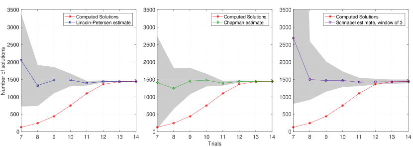
Figure 4: Estimates for solving Alt’s problem for four-bar linkages as the monodromy trials progressed using different estimates from left to right: Lincoln-Petersen, Chapman, and Schnabel using a window of size 3. The shaded area is the 95% confidence interval for each estimate.

5.2 Watt I six-bar mechanism

$N$	DOF	fixed pivots	# variables	# solutions	trace test	# other solutions
6	4	$A,B$	$50$	5754	Yes ($C$)	7167
7	2	$A$	$60$	198,614	Yes ($B$)	115,126
8	0	–	$70$	$\approx 1.68\cdot 10^{6}$	–	–

Table 1: Table of results for Watt I synthesis with $N$ task positions

The last collection of experiments arise from motion generation problems for Watt I six-bar linkages (Watt IB using the convention in [24]) following the formulation in [21]. For $N$ task positions, there are $16-2N$ degrees of freedom (DOF) so it is natural to specify one (when $N=7$) or both (when $N=6$) ground pivots as additional constraints. Table 1 summarizes the setup of the problems and results for $N=6,7,8$ task positions (see labels in Figure 1(a)). The $N=6,7$ cases were validated using the trace test applied to the first task position and the listed variable. For $N=8$, the number of solutions is estimated.

The $N=6$ case was considered in [21], [11], and [3] reporting 5735, 5743, and 5754 solutions, respectively. The trace test confirms the number of solutions is indeed 5754 with results of our monodromy loops and estimations presented in Figure 5. In particular, once monodromy loops returned over $25\%$ repeats, the estimations quickly converged to the number of solutions.

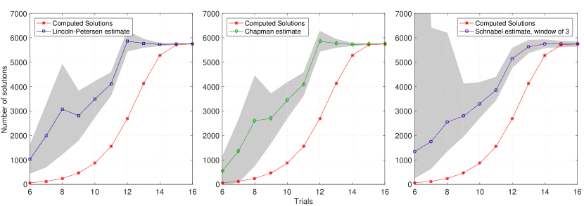
Figure 5: Estimates for Watt I synthesis with $N=6$ task positions and both pivots fixed as the monodromy trials progressed using different estimates from left to right: Lincoln-Petersen, Chapman, and Schnabel using a window of size 3. The shaded area is the 95% confidence interval for each estimate.

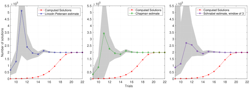
Figure 6: Estimates for Watt I synthesis with $N=7$ task positions and pivot $B$ fixed as the monodromy trials progressed using different estimates from left to right: Lincoln-Petersen, Chapman, and Schnabel using a window of size 3. The shaded area is the 95% confidence interval for each estimate.

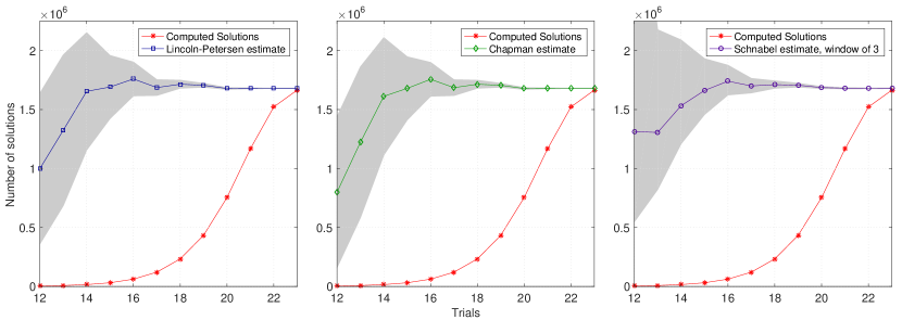
Figure 7: Estimates for Watt I synthesis with $N=8$ task positions as the monodromy trials progressed using different estimates from left to right: Lincoln-Petersen, Chapman, and Schnabel using a window of size 3. The shaded area is the 95% confidence interval for each estimate.

The estimations for $N=7$ with pivot $B$ fixed are shown in Figure 6 with the trace test validating the total number of solutions is 198,614. Once over 50% of the solutions were found, the estimate was within 1% of the actual number.

An estimate in [3] for the fully constrained motion generation problem with $N=8$ task positions is 840,300 cognate pairs, i.e., 1,680,600 distinct mechanisms, which is within the 95% confidence intervals of our results presented in Figure 7.

6 Conclusion

Linkage design in kinematics naturally leads to solving parameterized polynomial systems. A statistical estimation of the number of solutions to such systems was developed by using a capture-mark-recaputure model based on monodromy loops. This statistical method was demonstrated on Alt’s problem and several Watt I motion generation problems. The results show that the estimates quickly converge to the actual number of solutions once a reasonable proportion of the solutions have been found. A stopping criterion based on a multihomogeneous trace test is used to validate the completeness of the solution set.

References

- [1]
- [2] Alt, H.: Über die erzeugung gegebener ebener kurven mit hilfe des gelenkvierecks. ZAMM 3(1), 13–19 (1923)
- [3] Baskar, A., Bandyopadhyay, S.: An algorithm to compute the finite roots of large systems of polynomial equations arising in kinematic synthesis. Mechanism and Machine Theory 133, 493–513 (2019)
- [4] Bates, D.J., Hauenstein, J.D., Sommese, A.J., Wampler, C.W.: Bertini: Software for numerical algebraic geometry. Available at bertini.nd.edu
- [5] Bates, D.J., Hauenstein, J.D., Sommese, A.J., Wampler, C.W.: Numerically Solving Polynomial Systems with Bertini. Society for Industrial and Applied Mathematics (2013)
- [6] Bliss, N., Duff, T., Leykin, A., Sommars, J.: Monodromy solver: sequential and parallel. In: Proceedings of the 2018 ACM International Symposium on Symbolic and Algebraic Computation, pp. 87–94. Association for Computing Machinery (2018)
- [7] Brake, D.A., Hauenstein, J.D., Liddell, A.C.: Decomposing solution sets of polynomial systems using derivatives. In: G.M. Greuel, T. Koch, P. Paule, A. Sommese (eds.) Mathematical Software – ICMS 2016, pp. 127–135. Springer International (2016)
- [8] Chapman, D.G.: Some properties of the hypergeometric distribution with applications to zoological sample censuses. University of California Publications in Statistics 1(7), 131–159 (1951)
- [9] Duff, T., Hill, C., Jensen, A., Lee, K., Leykin, A., Sommars, J.: Solving polynomial systems via homotopy continuation and monodromy. IMA J. Numerical Analysis 39(3), 1421–1446 (2018)
- [10] Erdman, A.G., Sandor, G.N., Kota, S.: Mechanism Design: Analysis and Synthesis, 4th edn. Prentice Hall, Englewood Cliffs, N.J. (2001)
- [11] Glabe, J., McCarthy, J.: Six-bar linkage design system with a parallelized polynomial homotopy solver. In: Advances in Robot Kinematics 2018, pp. 133–140. Springer International (2019)
- [12] Hauenstein, J.D., Haywood, I., Liddell Jr., A.C.: An a posteriori certification algorithm for Newton homotopies. In: ISSAC 2014—Proceedings of the 39th International Symposium on Symbolic and Algebraic Computation, pp. 248–255. ACM, New York (2014)
- [13] Hauenstein, J.D., Oeding, L., Ottaviani, G., Sommese, A.J.: Homotopy techniques for tensor decomposition and perfect identifiability. Journal für die reine und angewandte Mathematik 2019(753), 1–22 (2019)
- [14] Hauenstein, J.D., Rodriguez, J.I.: Multiprojective witness sets and a trace test. Advances in Geometry (2020). To appear.
- [15] Hauenstein, J.D., Rodriguez, J.I., Sottile, F.: Numerical computation of Galois groups. Foundations of Computational Mathematics 18, 867–890 (2018)
- [16] Hauenstein, J.D., Wampler, C.W., Pfurner, M.: Synthesis of three-revolute spatial chains for body guidance. Mechanism and Machine Theory 110, 61–72 (2017)
- [17] Leykin, A., Rodriguez, J.I., Sottile, F.: Trace test. Arnold Math. Journal 4, 113–125 (2018)
- [18] McCarthy, J.M., Soh, G.S.: Geometric Design of Linkages, 2nd edn. Springer, New York (2001)
- [19] Morgan, A.P., Sommese, A.J.: Coefficient-parameter polynomial continuation. Appl. Math. Comput. 29(2, part II), 123–160 (1989)
- [20] Plecnik, M., Fearing, R.: Finding only finite roots to large kinematic synthesis systems. J. Mechanisms Robotics 9(2) (2017)
- [21] Plecnik, M., McCarthy, J., Wampler, C.: Kinematic synthesis of a watt i six-bar linkage for body guidance. In: Advances in Robot Kinematics, pp. 317–325. Springer International (2014)
- [22] Pollock, K., Nichols, J., Brownie, C., Hines, J.: Statistical inference for capture-recapture experiments. Wildlife Monographs 107, 3–97 (1990)
- [23] Seber, G.: The Estimation of Animal Abundance and Related Parameters. C. Griffin & Co., London (1982)
- [24] Sherman, S.N., Hauenstein, J.D., Wampler, C.W.: Curve cognate constructions made easy. IDETC-CIE (2020). To appear.
- [25] Sommese, A.J., Verschelde, J., Wampler, C.W.: Using monodromy to decompose solution sets of polynomial systems into irreducible components. In: Applications of algebraic geometry to coding theory, physics and computation (Eilat), NATO Sci. Ser. II Math. Phys. Chem., vol. 36, pp. 297–315. Kluwer Acad. Publ., Dordrecht (2001)
- [26] Sommese, A.J., Verschelde, J., Wampler, C.W.: Symmetric functions applied to decomposing solution sets of polynomial systems. SIAM J. Numer. Anal. 40(6), 2026–2046 (2002)
- [27] Sommese, A.J., Wampler, C.W.: The Numerical Solutions of Systems of Polynomials Arising in Science and Engineering. World Scientific Publishing Co. Pte. Lts., Hackensack, NJ (2005)
- [28] Wampler, C.W., Morgan, A.P., Sommese, A.J.: Complete solution of the 9-point path synthesis problem for 4-bar linkages. J. Mech. Des. 114, 153–159 (1992)
- [29] Wampler, C.W., Sommese, A.J.: Numerical algebraic geometry and algebraic kinematics. Acta Numer. 20, 469–567 (2011)
- [30]