Stochastic MPC with Distributionally Robust Chance Constraints

Abstract

In this paper we discuss distributional robustness in the context of stochastic model predictive control (SMPC) for linear time-invariant systems. We derive a simple approximation of the MPC problem under an additive zero-mean i.i.d. noise with quadratic cost. Due to the lack of distributional information, chance constraints are enforced as distributionally robust (DR) chance constraints, which we opt to unify with the concept of probabilistic reachable sets (PRS). For Wasserstein ambiguity sets, we propose a simple convex optimization problem to compute the DR-PRS based on finitely many disturbance samples. The paper closes with a numerical example of a double integrator system, highlighting the reliability of the DR-PRS w.r.t. the Wasserstein set and performance of the resulting SMPC.

Model Predictive Control (MPC) is an optimization based control strategy that has received a lot attention through academia and industry over the last couple of decades, mainly due to its ability to explicitly take constraints into account (Rawlings and Mayne, 2009).

In almost every practical application, the states of the system are falsified by disturbances, which result from e.g. measurement noise, process noise or model-plant mismatch. If one can give an a-priori bound on such disturbances, one may use a robust MPC framework (Mayne et al., 2005), which guarantees robust constraint satisfaction and robust stability. However, these approaches tend to be overly conservative, since the robustness is regarding worst-case disturbances, which may occur to a very low percentile.

If one has a model of the disturbance, e.g. the probability distribution, then the designer may use a stochastic MPC framework (Mesbah, 2016), which aims to find a trade-off between constraint satisfaction and controller performance. By constraint satisfaction we refer to chance constraints (Farina et al., 2016), which are a popular type of constraint relaxation technique, which enforces that the hard constraints have to be satisfied only with a certain probability. In many practical applications these kind of constraints are very beneficial, e.g. comfort constraints in a room temperature control scenario.

Stochastic MPC approaches can furthermore be separated into several sub categories. On the one hand there are scenario-based approaches (Schildbach et al., 2012) (Hewing and Zeilinger, 2019), which, at every time instant, sample sufficiently many disturbance realizations in order to approximate the stochastic control problem. The inherent sampling technique makes the scenario-based methods applicable for systems with arbitrary disturbances. However, due to their heavy computational load these methods are still limited to small scale systems. On the other hand we have analytical approximation methods (Farina et al., 2013) (Hewing et al., 2018) (Mark and Liu, 2019) (Mark and Liu, 2020), which assume a certain structure in the probability distribution in order to reformulate the stochastic problem based on the moments of the disturbance. These approaches are limited due to the necessity of the exact probability distribution, which, from a practical point of view, is usually not available.

Motivated by recent results on distributionally robust (DR) optimization (Esfahani and Kuhn, 2018), we try to seek a middle path in between scenario-based and analytical approximation methods, where we utilize Wasserstein ambiguity sets (Kuhn et al., 2019) in combination with indirect feedback SMPC (Hewing et al., 2018).

Related work:

In (Van Parys et al., 2015) the authors propose DR receding horizon and infinite horizon controllers for linear discrete time-invariant (DLTI) systems subject to additive disturbances. The DR chance constraints are approximated with conditional value-at-risk (CVaR) constraints and a moment-based ambiguity set. In (Darivianakis et al., 2017) the authors propose to use statistical hypothesis testing to construct probabilistic confidence bounds that replace the DR chance constraints as robust constraints.

Contribution:

In this paper we extend the framework of PRS to DR-PRS. This is achieved by rewriting the PRS by means of the union of convex loss functions and computing for each loss function the worst-case VaR, which is equivalent to the DR chance constraint formulation. For Wasserstein ambiguity sets we propose a data driven method to compute DR-PRS based on finite samples using a CVaR optimization problem of the error loss function.

Outline:

The paper is organized as follows. In the first section we introduce the DR problem setting. Section 2 introduces the MPC ingredients and the core of the paper, namely the reformulation of DR chance constraints as DR-PRS. In section 3 we present tractable results for worst-case VaR optimization problems whereas Section 4 closes the paper with two numerical examples on DR-PRS and an MPC implementation of a second order system. For the sake of readability all proofs can be found in the appendix.

Notation:

Given two polytopic sets $\mathbb{A}$ and $\mathbb{B}$, the Pontryagin difference is given as $\mathbb{A}\ominus\mathbb{B}=\{a\in\mathbb{A}:a+b\in\mathbb{A},\forall b\in\mathbb{B}\}$. The set of symmetric positive semidefinite (definite) matrices is defined as $\mathbb{S},\mathbb{S}_{+}$. Positive definite and semidefinite matrices are indicated as $A>0$ and $A\geq 0$, respectively. For an event $E$ we define the probability of occurrence as $\mathbb{P}(E)$, whereas $\mathbb{P}(E|D)$ denotes the conditional probability. We define for a random variable $w$ the expected value w.r.t. distribution $\mathbb{P}$ as $\mathbb{E}_{\mathbb{P}}(w)$. Given a measurable loss function $l(w)$ and a risk threshold $\epsilon\in(0,1)$, the VaR of $l(w)$ at level $\epsilon$ is defined as $\mathbb{P}\text{-VaR}_{\epsilon}(l(w))=\text{inf}[\gamma\in\mathbb{R}|\mathbb{P}\{\gamma\leq l(w)\}\leq\epsilon]$. The CVaR of $l(w)$ at level $\epsilon$ is given as $\mathbb{P}\text{-CVaR}_{\epsilon}(l(w))=\text{inf}[\tau+\epsilon^{-1}\mathbb{E}_{\mathbb{P}}\{\text{max}(0,l(w)-\tau)\}|\tau\in\mathbb{R}]$.

1 Problem formulation

We consider a discrete-time linear time-invariant system

$$x(k+1)=Ax(k)+Bu(k)+w(k)$$ (1)

with state $x\in\mathbb{R}^{n_{x}}$, input $u\in\mathbb{R}^{n_{u}}$ and independent and identically distributed (i.i.d.) white noise $w\in\mathbb{R}^{n_{x}}$. The states and inputs are subject to chance constraints

$$\mathbb{P}(x\in\mathbb{X}|x(0))\geq p_{x}$$ (2a)

$$\mathbb{P}(u\in\mathbb{U}|x(0))\geq p_{u},$$ (2b)

where the constraint sets $\mathbb{X}=\{x\in\mathbb{R}^{n_{x}}|Hx(k)\leq h\}$ and $\mathbb{U}=\{u\in\mathbb{R}^{n_{u}}|Lu(k)\leq l\}$ are convex polytopes that contain the origin in their interior with $h\in\mathbb{R}_{>0}^{n_{p}}$ and $l\in\mathbb{R}_{>0}^{n_{q}}$. The level of chance constraint satisfaction is regulated with $p_{x},p_{u}\in(0,1)$.

A common assumption in analytical SMPC approaches is that the statistics of the disturbance $w$ are known and so the probability measure $\mathbb{P}$. However, this is restrictive from a practical point of view, where the true distribution is usually unknown, i.e. it must be estimated from historical data. We make the following assumption.

Assumption 1.

• The true probability distribution $\mathbb{P}$ is light-tailed

• $\mathbb{P}$ belongs to an ambiguity set $\hat{\mathcal{P}}$ with probability $1-\beta$, where $\beta\in(0,1)$.

Remark 2.

An ambiguity set is a collection of plausible variations of the empirically estimated distribution, where the literature distinguishes roughly between discrepancy and moment-based ambiguity sets. We refer the interested reader to the recently published survey paper (Rahimian and Mehrotra, 2019) for a detailed overview.

To immunize (2) against distributional ambiguity, we state the following DR chance constraints

$$\!\inf_{\mathbb{Q}\in\hat{\mathcal{P}}}\mathbb{Q}(x\in\mathbb{X}|x(0))\geq p_{x}$$ (3a)

$$\!\inf_{\mathbb{Q}\in\hat{\mathcal{P}}}\mathbb{Q}(u\in\mathbb{U}|x(0))\geq p_{u}.$$ (3b)

The control objective is to approximately minimize the infinite horizon cost

$$J_{\infty}=\lim_{t\rightarrow\infty}\mathbb{E}_{\mathbb{P}}\bigg{\{}\frac{1}{t}\sum_{k=0}^{t}l(x(k),u(k))\bigg{\}},$$ (4)

where $l(x(k),u(k))$ denotes a stage cost function. To this end, we split system (1) into a deterministic nominal part $z(k)$ and a stochastic error part $e(k)$, such that $x(k)=z(k)+e(k)$. Following the lines of classic tube-based MPC, we introduce an affine error feedback controller $u(k)=v(k)+Ke(k)$, resulting in the decoupled dynamics

$$z(k+1) =Az(k)+Bv(k)$$ (5a)

$$e(k+1) =(A+BK)e(k)+w(k),$$ (5b)

where $K$ is the solution of the infinite horizon linear-quadratic control problem, such that $A_{K}\coloneqq A+BK$ is Schur stable. In this paper we use the recently proposed indirect feedback SMPC scheme from (Hewing et al., 2018), where the main advantage over classical SMPC approaches is the validity of (5b) in closed-loop under the MPC control law. For the treatment of DR chance constraints, we extend the concept of PRS to its DR counterpart for the error system (5b).

2 Distributionally Robust SMPC

In this section we introduce the controller structure, the MPC objective function and reformulate the DR chance constraints (3) in terms of a DR-PRS.

2.1 Controller structure

In the following we introduce the predictive dynamics for the MPC optimization problem, where we denote predicted quantities as e.g. $x(t|k)$ for a $t$-step ahead prediction of the state initialized at time step $k$. The predictive dynamics are

$$x(t+1|k)=Ax(t|k)+Bu(t|k)+w(t|k)$$ (6a)

$$z(t+1|k)=Az(t|k)+Bv(t|k)$$ (6b)

$$e(t+1|k)=(A+BK)e(t|k)+w(t|k),$$ (6c)

which are coupled to the closed-loop dynamics (1), (5) at each time step $k$ with $x(0|k)=x(k)$, $z(0|k)=z(k)$, $e(0|k)=e(k)$. The closed-loop error $e(k)$ is unaffected by the choice of $z(0|k)=z(k)$ and thus, evolves autonomously according to (5b) (Hewing and Zeilinger, 2019). For a quick overview, the following list gives insight in which quantities serve which purpose.

• The nominal dynamics (6b) serve as a prediction model for the MPC

• The predictive disturbance $w(t|k)$ and predictive error $e(t|k)$ are used to optimize the MPC cost

• The disturbance $w(k)$ and closed-loop error $e(k)$ are used to compute PRS for constraint tightening

The resulting input for system (1) is

$$u(k)=v^{*}(0|k)+Ke(0|k),$$ (7)

where $v^{*}(0|k)$ denotes the first element of the optimal input trajectory.

2.2 Objective

In order to minimize the infinite horizon cost (4), we consider a receding horizon strategy and solve the problem over a finite horizon of length $N$, where a terminal cost $V_{f}(x)$ is used to approximate the infinite horizon tail. The expected cost can then be written as

$$\mathbb{E}_{{\mathbb{Q}}}\{{J}_{k}(x,u)\}=\mathbb{E}_{{\mathbb{Q}}}\bigg{\{}V_{f}(x(N|k)+\sum_{t=0}^{N-1}l(x(t|k),u(t|k))\bigg{\}},$$ (8)

where the expectation $\mathbb{E}_{{\mathbb{Q}}}(\cdot)$ is taken w.r.t. the distribution ${\mathbb{Q}}$. A general way to solve optimization problems with expected cost functions akin to (8) are scenario approaches, e.g. (Hewing and Zeilinger, 2019), where the stochastic program is approximated with a sampling-average-approximation (SAA). The idea is to collect $M$ data samples $\mathcal{W}=\{w^{(1)},\ldots,w^{(M)}\}$ and replace $\mathbb{Q}$ with the empirical distribution $\hat{\mathbb{P}}\coloneqq M^{-1}\sum_{j\in\mathcal{W}}\delta_{w^{(j)}}$, where $\delta_{w^{(j)}}$ is the Dirac delta measure concentrated at $w^{(j)}$, such that (8) is approximated with $\mathbb{Q}=\hat{\mathbb{P}}$ as

$$\frac{1}{M}\sum_{i=1}^{M}\bigg{\{}V_{f}(x^{(i)}(N|k)+\sum_{t=0}^{N-1}l(x^{(i)}(t|k),u^{(i)}(t|k))\bigg{\}}.$$

Minimization of the above cost yields a control sequence $u^{*}(\cdot|k)$ that provides an upper bound of the in-sample performance for the data set $\mathcal{W}$. However, if we implement $u^{*}(0|k)$ to the real system (1), which introduces new (disturbance) samples, then the controller may show a poor out-of-sample performance $\mathbb{E}_{{\mathbb{P}}}\{{J}_{k}(x,u^{*})\}$, which is the real quantity of interest. To highlight the importance between these two performance criteria, we refer the reader to (Esfahani and Kuhn, 2018).

Remark 3.

The SAA converges almost surely to the true expectation $\mathbb{E}_{\mathbb{P}}\{\cdot\}$ as the data size $M$ tends to infinity (Esfahani and Kuhn, 2018). However, for small data sizes, the SAA performs poorly in regard to the out-of-sample performance and is the main motivation to consider DR optimization.

To robustify the MPC optimization problem against distributional uncertainty, we consider an ambiguity set $\hat{\mathcal{P}}$ to reformulate the cost (8) as

$$\!\sup_{\mathbb{Q}\in\hat{\mathcal{P}}}\mathbb{E}_{\mathbb{Q}}\bigg{\{}V_{f}(x(N|k)+\sum_{t=0}^{N-1}l(x(t|k),u(t|k))\bigg{\}},$$ (9)

which serves as an upper bound for the out-of-sample performance with high probability, i.e.

$${\mathbb{P}}\big{\{}\mathbb{E}_{{\mathbb{P}}}\{{J}_{k}(x,u)\}\leq\eqref{eq:dr_cost}\big{\}}\geq 1-\beta.$$ (10)

Quadratic cost with zero-mean i.i.d. noise

Since the main emphasize of this paper are DR chance constraints, we consider the special case of zero-mean i.i.d. disturbances under a quadratic cost function

$$l(x,u)=\|x\|^{2}_{Q}+\|u\|^{2}_{R},$$

where $Q\geq 0$, $R>0$ are weighting matrices for the states and inputs. The terminal cost function is given by

$$V_{f}(x)=\|x\|_{P}^{2}$$

with a positive definite weight $P>0$ that satisfies the Lyapunov equation $A_{K}^{\top}PA_{K}+Q+K^{\top}RK=P$. Note that the closed-loop error $e(k)$ is driven by the stochastic process (5b), which, under the zero-mean assumption on $w$ and the initialization of $e(0)=0$, is zero-mean. For the predicted error $e(t|k)$ this does not hold in general, which is due to the choice $e(0|k)=e(k)$. Therefore, the predicted state and input mean are given as $\mu_{x}=z(t|k)+A_{K}^{t}e(k)$ and $\mu_{u}=v(t|k)+KA_{K}^{t}e(k)$, such that (9) evaluates to

$$\!\sup_{\mathbb{Q}\in\hat{\mathcal{P}}}\mathbb{E}_{\mathbb{Q}}\bigg{\{}\|x(N|k)\|_{P}^{2}+\sum_{t=0}^{N-1}\|x(t|k)\|_{Q}^{2}+\|u(t|k)\|_{R}^{2}\bigg{\}}$$

$$=\|\mu_{x}(N|k)\|_{P}^{2}+\sum_{t=0}^{N-1}\|\mu_{x}(t|k)\|_{Q}^{2}+\|\mu_{u}(t|k)\|_{R}^{2}$$ (11a)

$$+\!\sup_{\mathbb{Q}\in\hat{\mathcal{P}}}\mathbb{E}_{\mathbb{Q}}\bigg{\{}\|e(N|k)\|_{P}^{2}+\sum_{t=0}^{N-1}\|e(t|k)\|_{Q^{*}}^{2}\bigg{\}}$$ (11b)

where $Q^{*}=Q+K^{\top}RK$. It can be seen that (11b) does not depend on the optimization variables $z,v$ and hence, is a neglectable constant in the optimization problem, which was also reported in (Hewing et al., 2018).

Remark 4.

Since (11b) does not depend on the MPC optimization variables $z,v$, the out-of-sample performance (9) cannot be improved through the MPC optimization problem. This changes if the underlying disturbance $w$ is non i.i.d. and non zero mean. However, DR performance could still be achieved by considering a DR tube-controller, see (Yang, 2018) for related results.

2.3 Distributionally robust chance constraints

The following section is dedicated to the reformulation of the DR chance constraints (3) in terms of a DR Probabilistic Reachable Set.

Definition 5.

A set $\mathbb{A}$ is a Distributionally Robust Probabilistic Reachable Set (DR-PRS) of probability level $p$ w.r.t. to the ambiguity set $\hat{\mathcal{P}}$ for system (5b) initialized with $e(0)=0$ if

$$\mathbb{Q}(e(k)\in\mathbb{A})\geq p\quad\forall\mathbb{Q}\in\hat{\mathcal{P}}\quad\forall k\geq 0$$

According to (Zymler et al., 2013) the DR-PRS condition $\mathbb{Q}(e(k)\in\mathbb{A})\geq p\quad\forall\mathbb{Q}\in\hat{\mathcal{P}}$ can similarly be rewritten as

$$\!\inf_{\mathbb{Q}\in\hat{\mathcal{P}}}\mathbb{Q}(e(k)\in\mathbb{A})\geq p\Leftrightarrow\!\sup_{\mathbb{Q}\in\hat{\mathcal{P}}}\mathbb{Q}(e(k)\notin\mathbb{A})\leq 1-p.$$ (12)

Remark 6.

A DR-PRS is a probabilistic confidence region, such that for all distributional variations over the ambiguity set $\hat{\mathcal{P}}$, any future (unseen) process realization $e(k)$ lies in $\mathbb{A}$ with a probability of at least $p$, i.e. the worst-case probability of $e(k)\notin\mathbb{A}$ is smaller that $1-p$.

Remark 7.

For time-varying or non zero-mean errors $e$ it is possible to consider time-varying DR-PRS for constraint tightening, i.e. for each time step $k$ we define a DR-PRS $\mathbb{A}_{k}$, such that

$$\!\inf_{\mathbb{Q}\in\hat{\mathcal{P}}}\mathbb{Q}(e(k)\in\mathbb{A}_{k})\geq p_{x}\quad\forall\mathbb{Q}\in\hat{\mathcal{P}}$$

Remark 8.

If $\hat{\mathcal{P}}$ is a singleton that contains only the true distribution $\mathbb{P}$, then the ambiguous free PRS, or simply PRS, $\mathbb{S}$ is recovered.

The DR-PRS allows for a direct reformulation of the closed-loop chance constraints (2), which is formalized in the following lemma.

Lemma 9.

Consider two polytopic DR-PRS for the states and inputs, i.e. $\mathbb{A}_{x}=\{He(k)\leq\eta_{x}\}$ and $\mathbb{A}_{u}=\{LKe(k)\leq\eta_{u}\}$. System (1) satisfies the DR chance constraints (3) for any $k\geq 0$ conditioned on $e(0)=x(0)-z(0)=0$ with a probability of at least $1-\beta$, if and only if the nominal system (6b) satisfies the constraints $z(k)\in\mathbb{Z}$ and $v(k)\in\mathbb{V}$ with

$$\mathbb{Z}=\mathbb{X}\ominus\mathbb{A}_{x}$$

$$\mathbb{V}=\mathbb{U}\ominus\mathbb{A}_{u}$$

The previous result gives insight in the connection between between DR-PRS and PRS, which is summarized in the following corollary.

Corollary 10.

Let $\mathbb{S}$ be a PRS and $\mathbb{A}$ a DR-PRS and let $\hat{\mathcal{P}}$ be an ambiguity set. If condition $\mathbb{P}({\mathbb{P}}\in\hat{\mathcal{P}})\geq 1-\beta$ is satisfied, then ${\mathbb{P}}\big{\{}\mathbb{S}\subseteq\mathbb{A}\}\geq 1-\beta$.

The main challenge in the DR-PRS synthesis poses the underlying worst-case VaR optimization problem (16). The worst-case VaR computation depends highly on the structure of the ambiguity set, e.g. if $\hat{\mathcal{P}}$ is replaced with a moment-based ambiguity set, then the results from (Zymler et al., 2013) can be used to express a DR-PRS. A similar result is reported by (Darivianakis et al., 2017), where the authors propose to use statistical hypothesis theory to define a compact DR confidence region to replace a moment-based ambiguity set. In this paper, we opt to solve the worst-case VaR over a Wasserstein ambiguity set, which is presented in Section 3.1.

2.4 Indirect feedback SMPC

Using the results from the previous sections, we can state the following MPC optimization problem.

$$\!\min_{v} \quad\eqref{eq:cost_simplified}$$ (13a)

s.t. $$\quad\mu_{x}(t+1|k)=z(t+1|k)+e(t+1|k),$$ (13b)

$$\quad z(t+1|k)=Az(t|k)+Bv(t|k),$$ (13c)

$$\quad e(t+1|k)=(A+BK)^{t}e(k),$$ (13d)

$$\quad\mu_{u}(t|k)=v(t|k)+Ke(t|k),$$ (13e)

$$\quad z(t|k)\in\mathbb{Z},v(t|k)\in\mathbb{V},z(N|k)\in\mathbb{Z}_{f}$$ (13f)

$$\quad\mu_{x}(0|k)=x(k),z(0|k)=z(k),e(0|k)=e(k)$$ (13g)

for all $t=0,\ldots,N-1$. For $k=0$ the nominal state is initialized with $z(0)=x(0)$. The result of the optimization problem is a sequence of nominal control inputs $v(t|k),t=\{0,\ldots,N-1\}$, whereas only the first element $v^{*}(0|k)$ is implemented with control law (7) to the real system (1) and the rest is discarded. Then the time step $k\leftarrow k+1$ increments and problem (13) is solved repeatedly. For the sake of simplicity we assume a zero terminal constraint, i.e. $\mathbb{Z}_{f}=\{0\}$. Recursive feasibility of problem (13) can be established with the standard procedure (shifted optimal cost and terminal controller), see (Hewing et al., 2018, Theorem 1) for details. Satisfaction of the DR chance constraints (with $1-\beta$ confidence) in closed-loop follows from Lemma 9 and (Hewing et al., 2018, Lemma 1), which states that the predicted error has the same distribution as the closed-loop error.

3 Tractable reformulations

The general ambiguity set $\hat{\mathcal{P}}$ is replaced with a Wasserstein ambiguity set, which is defined as a statistical ball of radius $\theta$ centered at the empirical distribution $\hat{\mathbb{P}}$, i.e.

$$\mathbb{B}_{\theta}(\hat{\mathbb{P}})=\{\mathbb{Q}\in\mathcal{P}(\mathbb{R})\>|\>d_{p}(\hat{\mathbb{P}}_{M},\mathbb{Q})\leq\theta\},$$ (14)

where $\mathcal{P}(\mathbb{R})$ is a set of Borel probability measures on $\mathbb{R}$, such that the expected value $\mathbb{E}_{\mathbb{Q}}(\|w\|_{p})$ under any norm $\|\cdot\|_{p}$ is finite. The measure $d_{p}(\mathbb{Q},\mathbb{P})$ denotes the $p$-Wasserstein distance.

Definition 11.

For any $p\in[1,\infty)$, the $p$-Wasserstein distance between two arbitrary distributions $\mathbb{Q}$ and $\mathbb{P}$ supported on $\mathbb{R}$ is defined as

$$d_{p}(\mathbb{Q},\mathbb{P})\coloneqq\!\inf_{\Xi}\bigg{(}\int_{\mathbb{R}^{2}}\|\xi-\xi^{\prime}\|_{p}\Xi(d\xi,d\xi^{\prime})\bigg{)}^{\frac{1}{p}},$$

where $\Xi$ is the set of all joint probability distribution of $\xi$ and $\xi^{\prime}$ with marginals $\mathbb{Q}$ and $\mathbb{P}$.

A Wasserstein radius $\theta$ for (14) that satisfies Assumption 1 can is formalized in the following theorem.

Theorem 12.

Let Assumption 1 hold with $\beta\in(0,1)$ and let $\hat{\mathcal{P}}=\mathbb{B}_{\theta}(\hat{\mathbb{P}})$. Then, for a given data size $M$, there exists an $\theta=\theta_{M}(\beta)>0$, such that (10) holds.

The proof of the above theorem follows from (Esfahani and Kuhn, 2018, Thm. 3.5) and more generally by (Fournier and Guillin, 2015, Thm. 2). The previous result highlights the main advantage of the Wasserstein ambiguity set compared to moment-based ambiguity sets, since it connects the data size $M$ to the size of the uncertainty set while maintaining the probabilistic guarantee $1-\beta$. Furthermore, the Wasserstein radius $\theta_{M}(\beta)$ is a monotonic decreasing function in the data size $M$, i.e. for $M\rightarrow\infty$, the Wasserstein ambiguity set reduces to the singleton that contains only the true distribution $\mathbb{P}$.

3.1 Worst-case Value-at-Risk

In this section we introduce a method to solve worst-case VaR problems that appear in the DR-PRS synthesis. We consider a set $\mathcal{E}=\{e^{(1)},\ldots,e^{(M)}\}$ that contains $M$ i.i.d. samples of the closed-loop error (5b) and use the marginal distribution in each direction of the error $e$ to define a symmetric box-shaped DR-PRS of the form

$$\mathbb{A}_{B}\coloneqq\{e\in\mathbb{R}^{n_{x}}\>|\>|e_{i}|\leq\eta_{i}\quad\forall i=1,\ldots,n_{x}\},$$

where $e_{i}$ denotes the $i$-th element of $e$. Using techniques from (Esfahani and Kuhn, 2018), the worst-case VaR $\eta_{i}$ of the $i$-th marginal distribution at probability level $\epsilon_{i}$ can be computed as a byproduct of the following worst-case CVaR optimization problem

$$\text{CVaR}_{\epsilon_{x}}(|e_{i}|)=\>\ \!\min_{\lambda\geq 0} \>\>\tilde{\eta}_{i}+\frac{1}{\epsilon_{i}}\bigg{(}\theta\lambda+\frac{1}{M}\sum_{j=1}^{M}\alpha_{j}\bigg{)}$$ (15a)

s.t. $$\quad\theta\lambda+\frac{1}{M}\sum_{j=1}^{M}\alpha_{j}\leq\epsilon_{i}$$ (15b)

$$\quad\alpha_{j}\geq(|e_{i}^{(j)}|-\tilde{\eta}_{i})^{+}\hskip 3.50006pt\forall j\in\mathcal{E}$$ (15c)

where $(|e_{i}^{(j)}|-\tilde{\eta}_{i})^{+}=\text{max}(0,|e_{i}^{(j)}|-\tilde{\eta}_{i})$. Note that for $\theta=0$, the optimization problem is equal to a SAA, i.e. the worst-case CVaR and worst-case VaR reduce to the CVaR and VaR based on the empirical distribution $\hat{\mathbb{P}}$. Furthermore, the Wasserstein penalty $\lambda$ can be increased arbitrarily without having an effect on $\eta_{i}$.

Remark 13.

The CVaR is a measure for the average loss above the $(1-\epsilon_{i})$-th quantile of the loss function, i.e. $\text{VaR}_{\epsilon}(|e_{i}|)\leq\text{CVaR}_{\epsilon}(|e_{i}|)$, as illustrated in Figure 1.

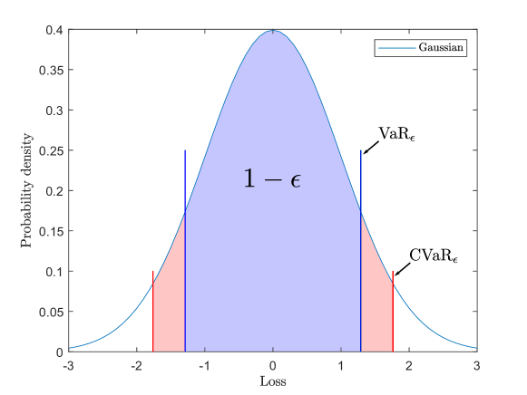
Figure 1: Box-shaped PRS with VaR and CVaR for a standard Gaussian distribution at probability level $p=0.8$.

4 Numerical example

This section is dedicated to a numerical example, highlighting the convergence and chance constraint satisfaction properties of the proposed approach. To compare our results, we utilize the double integrator example from (Hewing et al., 2018) with dynamics

$$x(k+1)=\begin{bmatrix}1&1\\ 0&1\end{bmatrix}x(k)+\begin{bmatrix}0.5\\ 1\end{bmatrix}u(k)+w(k),$$

where $w$ is a normally distributed zero-mean i.i.d. disturbance with true distribution

$$w\sim\mathcal{N}(0,\Sigma_{w}),\quad\Sigma_{w}=\begin{bmatrix}0.25&0.5\\ 0.5&1\end{bmatrix}.$$

We impose a chance constraint on the second state, i.e. $\mathbb{P}(|x_{2}(k)|\leq 1.2)\geq 0.8$. Furthermore, we chose the stabilizing controller $K=[-0.2,-0.6]$. The cost weighting matrices are given as $Q=I$, $R=1$ and the prediction horizon is $N=30$. For the sake of simplicity we use a zero terminal constraint, i.e. $\mathbb{Z}_{f}=\{0\}$.

4.1 Ambiguity set

In the first experiment we want to exemplify the impact of the Wasserstein radius on the reliability of the DR-PRS. First, we compute the true error distribution $\mathbb{P}=\mathcal{N}(0,\Sigma_{e})$, where $\Sigma_{e}$ solves the Lyapunov equation $\Sigma_{e}=A_{K}\Sigma_{e}A_{K}^{\top}+\Sigma_{w}$. Thus, the true PRS is given as

$$\mathbb{S}=\bigg{\{}e_{2}\in\mathbb{R}\>|\>|e_{2}|\leq\sqrt{[\Sigma_{e}]_{2,2}\mathcal{X}^{2}_{1}(0.8)}=1.53\bigg{\}},$$

where $\mathcal{X}^{2}_{1}(0.8)$ is the chi-squared distribution at probability level $0.8$ with $1$ degree of freedom. Then we samples $N_{v}=10^{5}$ error states and store them as validation data. Now we consider three different data sizes $M=\{30,100,400\}$, where for each data size, $N_{mc}=1000$ DR-PRS are computed via (15) with $\epsilon_{x}=0.2$. For a given $\theta$ the reliability of the $i$-th DR-PRS is given by

$$\tilde{p}_{i}=\frac{1}{N_{v}}\sum_{j=1}^{N_{v}}\mathds{1}\big{\{}|e_{2}^{(j)}|\leq\eta_{x}(\theta)\big{\}}\quad\forall i\in\{1,\ldots,N_{mc}\}$$

where $\mathds{1}\{\cdot\}$ is the indicator function. We made explicit that $\eta_{x}(\theta)$ depends on $\theta$. The reliability of the Wasserstein radius $\theta$ w.r.t. the validation data is given by

$$r(\theta)=\frac{1}{N_{mc}}\sum_{i=1}^{N_{mc}}\mathds{1}\{\tilde{p}_{i}\geq 0.8\}.$$

Using the former empirical procedure, we compute the reliability for many Wasserstein radii in the interval $0\leq\theta\leq 0.2$ and summarized the results in Figure 2.

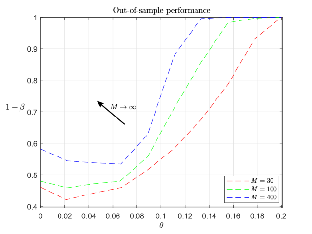
Figure 2: DR-PRS out-of-sample performance for many Wasserstein radii and data sizes $M=\{30,100,400\}$.

In Figure 3 we plot the corresponding quantiles over the Wasserstein radius.

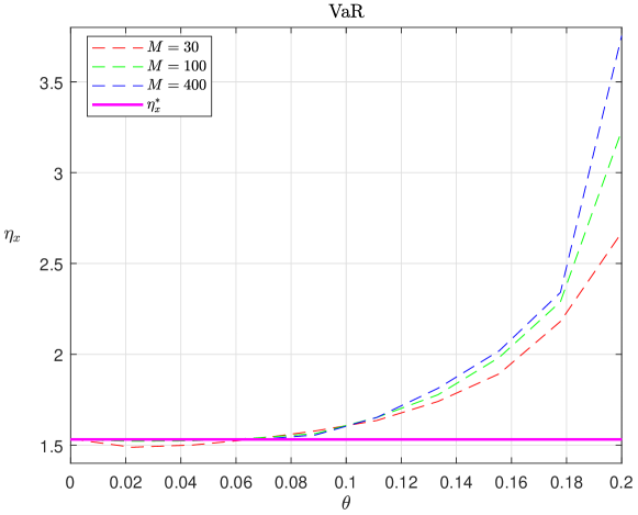
Figure 3: Quantiles for the data sizes $M=\{30,100,400\}$. The magenta line depicts the true VaR $\eta_{x}^{*}$ = 1.53.

In Figure 2 it can be observed that the reliability of the VaR estimate depends on the data size $M$ and the Wasserstein radius $\theta$. First we consider the ambiguous free case where $\theta=0$, which equals a sampling average approximation with the training data set. For small sample sizes the variance of $\eta(\theta)$ is large, which can be seen in Figure 3 for $\theta=0$, where the true quantile is approximated empirically via $N_{mc}=1000$ Monte-carlo simulations, but the reliability of that estimate is merely $46\%$. For increasing data sizes $M$, the variance of ${\eta}_{x}(\theta)$ is reduced, e.g. for $M=400$ the reliability of the same estimate is $58\%$. This verifies the statement of Remark 3 that the SAA performs poorly for small data sizes.

For $\theta>0$ the reliability of the estimate can be controlled, e.g. for $M=30$ a radius of $\theta=0.2$ is mandatory to guarantee a $99\%$ confidence, whereas for $M=400$ a radius of $\theta=0.131$ is sufficient. Thus, it is evident that a $1-\beta$ confidence can be maintained while reducing the Wasserstein radius as the data size $M$ increases. In practice, the Wasserstein radius should initially be set to a large value and successively be reduced by observing the number of constraint violations.

4.2 SMPC results

Now we implement three DR-PRS with an empirical reliability of $1-\beta=0.99$ with $\eta_{x}^{30}=2.67$, $\eta_{x}^{100}=2.14$, $\eta_{x}^{400}=1.8$ and run for each set $N_{s}=1000$ Monte-carlo simulations of $100$ closed-loop time steps. The initial state is given by $x(0)=[10,0]^{\top}$. We compare the average closed-loop cost (Av[J]) and the number of empirical constraints violations ($\#C_{\text{vio}}$) with the indirect feedback SMPC based on full distributional information with $\eta_{x}^{*}=1.53$.

Table 1: Performance for different PRS parameterizations

PRS	$\eta_{x}^{30}$	$\eta_{x}^{100}$	$\eta_{x}^{400}$	$\eta_{x}^{*}$
Av[J]	-	9.65	8.37	7.80
$\#C_{\text{vio}}$	-	1091	1169	1229

For $\eta_{x}^{30}$ the SMPC is infeasible for the initial state, which can be seen in Figure 4, where we compare the feasible regions for each DR-PRS and true PRS.

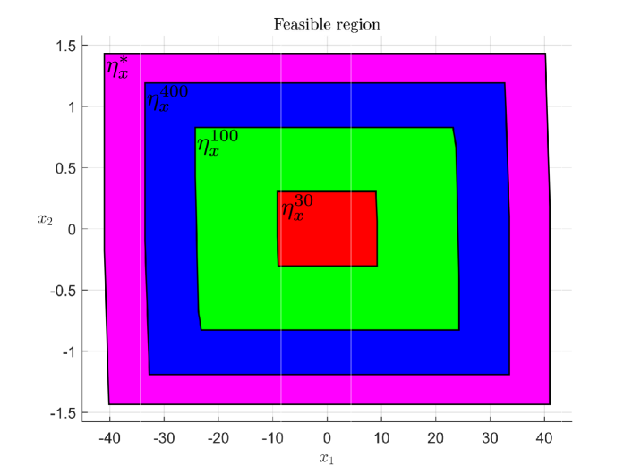
Figure 4: Feasible regions for different DR-PRS.

From Table 1 it is evident that for increasing data, the average MPC performance will converge to the true cost of around $7.80$. The same argument holds true for the number of constraint violations, which are all above the required level of $p_{x}=0.8$.

5 Conclusion

In this paper, we presented a SMPC based on indirect feedback with distributionally robust probabilistic reachable sets. We first robustified the MPC cost against distributional ambiguity and observed that for zero-mean i.i.d. disturbances the out-of-sample performance of the MPC cannot be improved through the MPC decision variables. Afterwards, the classical chance constraints got robustified against distributional ambiguity by means of a DR-PRS. The paper closed with two numerical examples, highlighting the out-of-sample performance of the DR-PRS and the closed-loop performance of the resulting SMPC.

Appendix A Proof of Lemma 9

Consider the state constraints (3) in polytopic form $Hx(k)\leq h$ conditioned on $x(0)$, which can equivalently be written as

$$\!\inf_{\mathbb{Q}\in\hat{\mathcal{P}}}\mathbb{Q}\bigg{(}\bigcap_{i=1}^{n_{p}}\big{\{}H_{i}x(k)\leq h_{i}\big{\}}\bigg{)}\geq p_{x}\\ \stackrel{{\scriptstyle\eqref{eq:equivalence_inf_sup}}}{{\Longleftrightarrow}}\!\sup_{\mathbb{Q}\in\hat{\mathcal{P}}}\mathbb{Q}\bigg{(}\bigcup_{i=1}^{n_{p}}\big{\{}H_{i}x(k)\geq h_{i}\big{\}}\bigg{)}\leq 1-p_{x},$$

where $H_{i}$ denotes the $i$-th row of $H$ and $h_{i}$ the $i$-th element of $h$. By substitution of $x=z+e$ and application of the union bound we obtain

$$\!\sup_{\mathbb{Q}\in\hat{\mathcal{P}}}\mathbb{Q}\bigg{(}\bigcup_{i=1}^{n_{p}}\big{\{}H_{i}x(k)\geq h_{i}\big{\}}\bigg{)}$$

$$\leq\sum_{i=1}^{n_{p}}\!\sup_{\mathbb{Q}\in\hat{\mathcal{P}}}\mathbb{Q}\{H_{i}z(k)+H_{i}e(k)\geq h_{i}\}\leq\sum_{i=1}^{n_{p}}\epsilon_{x,i}.$$

The individual violation probabilities $\epsilon_{x,i}\in(0,1)$ satisfy the condition $\sum_{i=1}^{n_{p}}\epsilon_{x,i}\leq\epsilon_{x}=1-p_{x}$. Furthermore,

$$\!\sup_{\mathbb{Q}\in\hat{\mathcal{P}}}\mathbb{Q}\big{\{}H_{i}z(k)+H_{i}e(k)-h_{i}\geq 0\big{\}}\leq\epsilon_{x,i}$$

$$\Longleftrightarrow \!\sup_{\mathbb{Q}\in\hat{\mathcal{P}}}\mathbb{Q}\text{-VaR}_{\epsilon_{x,i}}\big{\{}H_{i}z(k)+H_{i}e(k)-h_{i}\big{\}}\leq 0$$

$$\Longleftrightarrow H_{i}z(k)\leq h_{i}-\underbrace{\!\sup_{\mathbb{Q}\in\hat{\mathcal{P}}}\mathbb{Q}\text{-VaR}_{\epsilon_{x,i}}\big{\{}H_{i}e(k)\big{\}}}_{\coloneqq\eta_{x,i}}$$ (16)

where the first equivalence follows from the connection between the worst-case VaR and DR chance constraints (Zymler et al., 2013) and the second equivalence is due to the translational invariance of the VaR. The worst-case VaR in (16) can be computed as

$$\eta_{x,i}=\>\> \!\min_{\tilde{\eta}\in\mathbb{R}} \quad\tilde{\eta}$$ (17a)

s.t. $$\quad\!\sup_{\mathbb{Q}\in\hat{\mathcal{P}}}\mathbb{Q}(H_{i}e\geq\tilde{\eta})\leq\epsilon_{x,i}.$$ (17b)

By definition, the VaR $\eta_{x,i}$ coincides with the $(1-\epsilon_{x,i})$-th quantile of $H_{i}e(k)$. The DR-PRS is obtained by defining $\mathbb{A}_{x}=\{He\leq\eta_{x}\}$. To summarize, we established that

$$p_{x}\leq \!\inf_{\mathbb{Q}\in\hat{\mathcal{P}}}\mathbb{Q}(e(k)\in\mathbb{A}_{x})=\!\inf_{\mathbb{Q}\in\hat{\mathcal{P}}}\mathbb{Q}(x(k)-z(k)\in\mathbb{A}_{x})$$

$$= \!\inf_{\mathbb{Q}\in\hat{\mathcal{P}}}\mathbb{Q}(x(k)\in\{z(k)\}\oplus\mathbb{A}_{x})\leq\!\inf_{\mathbb{Q}\in\hat{\mathcal{P}}}\mathbb{Q}(x(k)\in\mathbb{X})$$

where the last inequality follows from $z(k)\in\mathbb{Z}$ and

$$(\underbrace{\mathbb{X}\ominus\mathbb{A}_{x}}_{\mathbb{Z}})\oplus\mathbb{A}_{x}\subseteq\mathbb{X}.$$

Recall that the ambiguity set $\hat{\mathcal{P}}$ itself is a random object, such that the true distribution $\mathbb{P}$ belongs only with $1-\beta$ confidence to $\hat{\mathcal{P}}$ (see Assumption 1). Thus, it immediately follows that

$${\mathbb{P}}\bigg{\{}\!\inf_{\mathbb{Q}\in\hat{\mathcal{P}}}\mathbb{Q}(x(k)\in\mathbb{X})\geq p_{x}\bigg{\}}\geq 1-\beta.$$

This concludes the proof for the DR state chance constraints (3a). The DR input chance constraints are similarly derived, starting from $Lu(k)\leq l$ and separation $Lv(k)+LKe(k)\leq l$. ∎

Appendix B Proof of Corollary 10

Assume that $\mathbb{P}({\mathbb{P}}\in\hat{\mathcal{P}})\geq 1-\beta=\tilde{\beta}$ is satisfied. From the proof of Lemma 9 we already know that the DR-PRS $\mathbb{A}$ is the result of a worst-case VaR optimization problem for each halfspace constraint. Now, for each $i\in\{1,\ldots,n_{p}\}$, we have

$$\mathbb{P}\bigg{\{}\mathbb{P}\text{-VaR}_{\epsilon_{x,i}}\{H_{i}e(k)\}\leq\!\sup_{\mathbb{Q}\in\hat{\mathcal{P}}}\mathbb{Q}\text{-VaR}_{\epsilon_{x,i}}\big{\{}H_{i}e(k)\}\bigg{\}}\geq\tilde{\beta},$$

which is a direct consequence of the probabilistic guarantee of the ambiguity set. The claim follows by taking the union bound and changing to set notation. ∎

References

- Darivianakis et al. (2017) Darivianakis, G., Georghiou, A., Smith, R.S., and Lygeros, J. (2017). The power of diversity: Data-driven robust predictive control for energy-efficient buildings and districts. IEEE Transactions on Control Systems Technology, 27(1), 132–145.
- Esfahani and Kuhn (2018) Esfahani, P.M. and Kuhn, D. (2018). Data-driven distributionally robust optimization using the wasserstein metric: Performance guarantees and tractable reformulations. Mathematical Programming, 171(1-2), 115–166.
- Farina et al. (2013) Farina, M., Giulioni, L., Magni, L., and Scattolini, R. (2013). A probabilistic approach to model predictive control. In 52nd IEEE Conference on Decision and Control, 7734–7739. IEEE.
- Farina et al. (2016) Farina, M., Giulioni, L., and Scattolini, R. (2016). Stochastic linear model predictive control with chance constraints–a review. Journal of Process Control, 44, 53–67.
- Fournier and Guillin (2015) Fournier, N. and Guillin, A. (2015). On the rate of convergence in wasserstein distance of the empirical measure. Probability Theory and Related Fields, 162(3-4), 707–738.
- Hewing et al. (2018) Hewing, L., Wabersich, K.P., and Zeilinger, M.N. (2018). Recursively feasible stochastic model predictive control using indirect feedback. arXiv preprint arXiv:1812.06860.
- Hewing and Zeilinger (2019) Hewing, L. and Zeilinger, M.N. (2019). Scenario-based probabilistic reachable sets for recursively feasible stochastic model predictive control. IEEE Control Systems Letters, 4(2), 450–455.
- Kuhn et al. (2019) Kuhn, D., Esfahani, P.M., Nguyen, V.A., and Shafieezadeh-Abadeh, S. (2019). Wasserstein distributionally robust optimization: Theory and applications in machine learning. In Operations Research & Management Science in the Age of Analytics, 130–166. INFORMS.
- Mark and Liu (2019) Mark, C. and Liu, S. (2019). Distributed stochastic model predictive control for dynamically coupled linear systems using probabilistic reachable sets. In 2019 18th European Control Conference (ECC), 1362–1367. IEEE.
- Mark and Liu (2020) Mark, C. and Liu, S. (2020). A stochastic output-feedback mpc scheme for distributed systems. arXiv preprint arXiv:2001.10838.
- Mayne et al. (2005) Mayne, D.Q., Seron, M.M., and Raković, S. (2005). Robust model predictive control of constrained linear systems with bounded disturbances. Automatica, 41, 219–224.
- Mesbah (2016) Mesbah, A. (2016). Stochastic model predictive control: An overview and perspectives for future research. IEEE Control Systems Magazine, 36(6), 30–44.
- Rahimian and Mehrotra (2019) Rahimian, H. and Mehrotra, S. (2019). Distributionally robust optimization: A review. arXiv preprint arXiv:1908.05659.
- Rawlings and Mayne (2009) Rawlings, J.B. and Mayne, D.Q. (2009). Model predictive control: Theory and design. Nob Hill Pub.
- Schildbach et al. (2012) Schildbach, G., Calafiore, G.C., Fagiano, L., and Morari, M. (2012). Randomized model predictive control for stochastic linear systems. In 2012 American Control Conference (ACC), 417–422. IEEE.
- Van Parys et al. (2015) Van Parys, B.P., Kuhn, D., Goulart, P.J., and Morari, M. (2015). Distributionally robust control of constrained stochastic systems. IEEE Transactions on Automatic Control, 61(2), 430–442.
- Yang (2018) Yang, I. (2018). Wasserstein distributionally robust stochastic control: A data-driven approach. arXiv preprint arXiv:1812.09808.
- Zymler et al. (2013) Zymler, S., Kuhn, D., and Rustem, B. (2013). Distributionally robust joint chance constraints with second-order moment information. Mathematical Programming, 137(1-2), 167–198.