Sub-chord diagrams of knot projections

Abstract.

A chord diagram is a circle with paired points with each pair of points connected by a chord. Every generic immersed spherical curve provides a chord diagram by associating each chord with two preimages of a double point. Any two spherical curves can be related by a finite sequence of three types of local replacement RI, RI​I, and RI​I​I, called Reidemeister moves. This study counts the difference in the numbers of sub-chord diagrams embedded in a full chord diagram of any spherical curve by applying one of the moves RI, strong RI​I, weak RI​I, strong RI​I​I, and weak RI​I​I defined by connections of branches related to the local replacements (Theorem 1). This yields a new integer-valued invariant under RI and strong RI​I​I that provides a complete classification of prime reduced spherical curves with up to at least seven double points (Theorem 2, Fig. 24): there has been no such invariant before. The invariant expresses the necessary and sufficient condition that spherical curves can be related to a simple closed curve by a finite sequence of RI and strong RI​I​I moves (Theorem 3). Moreover, invariants of spherical curves under flypes are provided by counting sub-chord diagrams (Theorem 4).

1. Introduction.

Any two knot projections (equivalently, generic immersed spherical curves) are related by a finite sequence of three types of local replacement, RI, RI​I, and RI​I​I, called Reidemeister moves, on knot projections. These replacements are defined by Fig. 1.

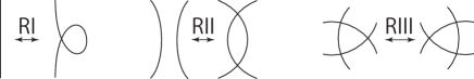
Figure 1. Reidemeister moves RI, RI​I, and RI​I​I from the left.

A chord diagram is a circle with chords with endpoints at different places on the circle. Chord diagrams are often used to study knots or knot projections. A chord diagram $CD_{P}$ of a knot projection, $P$, is a circle with the preimages of double points for which every pair of double-point preimages is connected by an arc. Examples are shown in the leftmost columns of Figs. 22 and 23. In this paper, a sub-chord diagram of $CD_{P}$ is a chord diagrams embedded in $CD_{P}$.

This paper exhibits characteristics of chord diagrams $\otimes$, , , and under five types of Reidemeister moves. In particular, we split the second (resp., third) Reidemeister move into the strong and weak second (resp., third) Reidemeister moves, as follows. The strong (resp., weak) second Reidemeister move, strong RI​I (resp., weak RI​I), is defined as the local replacement in Fig. 2.

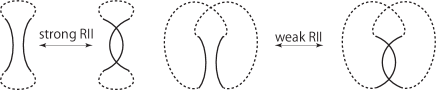
Figure 2. Strong (left) and weak (right) second Reidemeister moves. Dotted arcs indicate the connections of the branches.

The strong (resp., weak) third Reidemeister move, strong RI​I​I (resp., weak RI​I​I), is defined as the local replacement in Fig. 3.

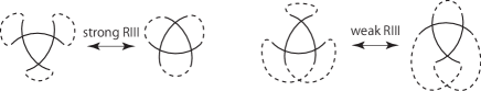
Figure 3. Strong (left) and weak (right) third Reidemeister moves. Dotted arcs indicate the connections of the branches.

Now we state some new results. Theorem 2 gives a new integer-valued invariant $\lambda(P)$ that provides a complete classification of all prime reduced knot projections with up to seven double points under the equivalence relation induced by RI and strong RI​I​I (strong (1, 3) homotopy [3]), as shown in Fig. 24. Throughout this paper, let $x(P)$ be the number of sub-chord diagrams, each of which is a chord diagram $x=\otimes,\begin{picture}(10.0,5.0)\put(5.0,3.0){\circle{7.0}} \qbezier(5.0,0.0)(5.0,3.0)(5.0,6.0)\qbezier(2.0,1.0)(5.0,3.0)(8.0,5.0)\qbezier(8.0,1.0)(5.0,3.0)(2.0,5.0)\end{picture}$, , , or in $CD_{P}$ of an arbitrary knot projection $P$.

Theorem 1.

The increments or decrements under one first, weak second, strong second, weak third, and strong third Reidemeister moves are shown in Fig. 4, respectively, where $m$ is an integer.

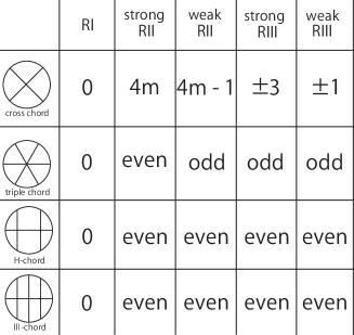
Figure 4. Difference under several types of Reidemeister moves. $m$ is an integer.

Theorem 2 is based on Theorem 1 and the discussion preceding it.

Theorem 2.

$$[3\begin{picture}(10.0,5.0)\put(5.0,3.0){\circle{7.0}} \qbezier(1.5,3.0)(5.0,3.0)(8.5,3.0)\qbezier(4.0,0.0)(4.0,3.0)(4.0,6.0)\qbezier(6.0,0.0)(6.0,3.0)(6.0,6.0)\end{picture}(P)-3\begin{picture}(10.0,5.0)\put(5.0,3.0){\circle{7.0}} \qbezier(5.0,0.0)(5.0,3.0)(5.0,6.0)\qbezier(2.0,1.0)(5.0,3.0)(8.0,5.0)\qbezier(8.0,1.0)(5.0,3.0)(2.0,5.0)\end{picture}(P)+\otimes(P)]/4$$

is an integer $\lambda(P)$ that is invariant under RI and strong RI​I​I.

We remark that there has been no non-trivial integer-valued invariant, such as $\lambda(P)$, under RI and strong RI​I​I before. The invariant $\lambda(P)$ is additive (Proposition 1) and has the following important properties.

Below, using the invariant $H(P)$ defined in [3] and introducing $\widetilde{X}(P)$, we have the following result, when $\lambda(P)=0$ (note that $\lambda(P)=0$ if $\widetilde{X}(P)=0$).

Theorem 3.

Let $P$ be an arbitrary knot projection. A map $H$ $($resp., $\widetilde{X}$$)$ from the set of all the knot projections to $\{0,1\}$ is defined by the condition $H(P)=0$ $($resp. $\widetilde{X}(P)=0$$)$ if and only if $\begin{picture}(10.0,5.0)\put(5.0,3.0){\circle{7.0}} \qbezier(1.5,3.0)(5.0,3.0)(8.5,3.0)\qbezier(4.0,0.0)(4.0,3.0)(4.0,6.0)\qbezier(6.0,0.0)(6.0,3.0)(6.0,6.0)\end{picture}(P)=0$ $($resp., $\otimes(P)=0$$)$. Then $H(P)$ $($resp., $\widetilde{X}(P)$$)$ is invariant under RI and strong RI​I​I $($resp., weak RI​I​I$)$ and we have the following four necessary and sufficient conditions:

$$H(P)=0~{}{\text{and}}~{}\lambda(P)=0 \Leftrightarrow{\text{$P$ can be related to $\begin{picture}(10.0,5.0)\put(5.0,3.0){\circle{8.0}} \end{picture}$ by using RI and strong RI\!I\!I,}}$$

$$\begin{picture}(10.0,5.0)\put(5.0,3.0){\circle{7.0}} \qbezier(5.0,0.0)(5.0,3.0)(5.0,6.0)\qbezier(2.0,1.0)(5.0,3.0)(8.0,5.0)\qbezier(8.0,1.0)(5.0,3.0)(2.0,5.0)\end{picture}(P)=0~{}{\text{and}}~{}\lambda(P)=0 \Leftrightarrow{\text{$P$ can be related to $\begin{picture}(10.0,5.0)\put(5.0,3.0){\circle{8.0}} \end{picture}$ by using RI,}}$$

$$\widetilde{X}(P)=0 \Leftrightarrow{\text{$P$ can be related to $\begin{picture}(10.0,5.0)\put(5.0,3.0){\circle{8.0}} \end{picture}$ by using RI and weak RI\!I\!I,}}~{}{\text{and}}~{}$$

$$\widetilde{X}(P)=0 \Leftrightarrow{\text{$P$ can be related to $\begin{picture}(10.0,5.0)\put(5.0,3.0){\circle{8.0}} \end{picture}$ by using RI}}$$

where denotes a simple closed curve on a sphere.

We also focus on sub-chord diagrams $\otimes$, , , , and , each of which has an invariance property under fylpes, where a flype is a local replacement on knot projections as shown in Fig. 5.

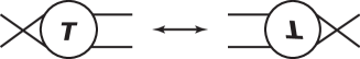
Figure 5. Flype.

Theorem 4.

$\otimes(P)$, $\begin{picture}(10.0,5.0)\put(5.0,3.0){\circle{7.0}} \qbezier(5.0,0.0)(5.0,3.0)(5.0,6.0)\qbezier(2.0,1.0)(5.0,3.0)(8.0,5.0)\qbezier(8.0,1.0)(5.0,3.0)(2.0,5.0)\end{picture}(P)$, $\begin{picture}(10.0,5.0)\put(5.0,3.0){\circle{7.0}} \qbezier(1.5,3.0)(5.0,3.0)(8.5,3.0)\qbezier(4.0,0.0)(4.0,3.0)(4.0,6.0)\qbezier(6.0,0.0)(6.0,3.0)(6.0,6.0)\end{picture}(P)$, $\begin{picture}(10.0,5.0)\put(5.0,3.0){\circle{7.0}} \qbezier(1.5,3.0)(5.0,3.0)(8.5,3.0)\qbezier(3.0,0.0)(3.0,3.0)(3.0,5.5)\qbezier(5.0,-0.5)(5.0,3.0)(5.0,6.5)\qbezier(7.0,0.0)(7.0,3.0)(7.0,5.5)\end{picture}(P)$, and $\begin{picture}(10.0,5.0)\put(5.0,3.0){\circle{7.0}} \qbezier(1.8,4.0)(5.0,4.0)(8.0,4.0)\qbezier(1.8,2.0)(5.0,2.0)(8.0,2.0)\qbezier(4.0,-0.2)(4.0,3.0)(4.0,6.0)\qbezier(6.0,-0.2)(6.0,3.0)(6.0,6.0)\end{picture}(P)$ are invariant under any flype.

Corollary 1.

$\lambda(P)$ is invariant under any flype.

The remainder of this paper contains the following sections. Theorem 1, 2, 3, and 4 are proved in Secs. 2, 3, 4 and 5, respectively. Sec. 4 also mentions properties of $\lambda$, and Sec. 6 comments on the behavior of Averaged invariant $-(J^{+}+2St)/2$ consisting of Arnold’s invariants $J^{+}$ and $St$. Finally, we present a table of prime reduced knot projections with up to seven double points, counting each type of sub-chord diagram embedded in a chord diagram of each knot projection.

2. Proof of Theorem 1.

Proof.

The sub-chord diagrams $\otimes$, , , and are called a cross chord, a triple chord, an H-chord, and a I​I​I-chord, respectively. Throughout this proof, $\Delta ch$ and $\Delta ch(x)$ are the difference of two numbers of embedded sub-chord diagrams and of embedded sub-chord diagrams specified by $x$, respectively, under a single local move that we focus on, where $x$ $=$ $\otimes$, , , and .

1. RI (Fig. 6). Consider the first column of the table in Fig. 4. Move RI does not affect $\otimes(P)$, $\begin{picture}(10.0,5.0)\put(5.0,3.0){\circle{7.0}} \qbezier(5.0,0.0)(5.0,3.0)(5.0,6.0)\qbezier(2.0,1.0)(5.0,3.0)(8.0,5.0)\qbezier(8.0,1.0)(5.0,3.0)(2.0,5.0)\end{picture}(P)$, $\begin{picture}(10.0,5.0)\put(5.0,3.0){\circle{7.0}} \qbezier(1.5,3.0)(5.0,3.0)(8.5,3.0)\qbezier(4.0,0.0)(4.0,3.0)(4.0,6.0)\qbezier(6.0,0.0)(6.0,3.0)(6.0,6.0)\end{picture}(P)$, or $\begin{picture}(10.0,5.0)\put(5.0,3.0){\circle{7.0}} \qbezier(1.5,3.0)(5.0,3.0)(8.5,3.0)\qbezier(3.0,0.0)(3.0,3.0)(3.0,5.5)\qbezier(5.0,-0.5)(5.0,3.0)(5.0,6.5)\qbezier(7.0,0.0)(7.0,3.0)(7.0,5.5)\end{picture}(P)$ for an arbitrary knot projection $P$. This implies that $\Delta ch=0$ for every box in the first column.

   

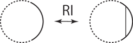
   Figure 6. RI on chord diagrams.

2. Strong RI​I (Fig. 7). Consider the second column of the table in Fig. 4. We separate the cases based on the number of chords that relate to a strong RI​I and belong to the new chord from the left to the right in Fig. 7.

   

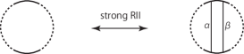
   Figure 7. Strong RI​I on chord diagrams.

   • $\otimes$. Any cross chord as a sub-chord cannot contain both chords $\alpha$ and $\beta$ in Fig. 7. Additionally, a chord crossing $\alpha$ (resp., $\beta$) should also cross $\beta$ (resp., $\alpha$). We will call this type of the argument the duality $(\alpha,\beta)$. Thus, the difference in $\otimes(P)$ of a knot projection $P$ by one strong RI​I should be even. Moreover, $\Delta ch(\otimes)=4m~{}(m\in\mathbb{Z})$. The reason is as follows.

     See Fig. 8. For any knot projection $P$, if $P$ has $\alpha$ on the right of Fig. 8, then the number of chords of $CD_{P}$ crossing $\alpha$ of $CD_{P}$ in the left figure of Fig. 8 is even. This is because for two component spherical curves, if a component of an immersed spherical curve intersects another component, the number of double points consisting of two components is even (Fig. 9).

     

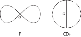
     Figure 8. Correspondence between a double point of a knot projection $P$ and a chord of chord diagram $CD_{P}$.

     

     Figure 9. Smoothing at a double point. The number of intersections of two dotted knot projections is even.

     By referring either $\alpha$ or $\beta$ to $\alpha$ of Fig. 8, $\Delta ch(\otimes)=4m~{}(m\in\mathbb{Z})$.

   • , , and . Since one strong RI​I consists of two RIs, a strong RI​I​I, and a weak RI​I, then $\Delta ch(\begin{picture}(10.0,5.0)\put(5.0,3.0){\circle{7.0}} \qbezier(5.0,0.0)(5.0,3.0)(5.0,6.0)\qbezier(2.0,1.0)(5.0,3.0)(8.0,5.0)\qbezier(8.0,1.0)(5.0,3.0)(2.0,5.0)\end{picture})=$ even, $\Delta ch(\begin{picture}(10.0,5.0)\put(5.0,3.0){\circle{7.0}} \qbezier(1.5,3.0)(5.0,3.0)(8.5,3.0)\qbezier(4.0,0.0)(4.0,3.0)(4.0,6.0)\qbezier(6.0,0.0)(6.0,3.0)(6.0,6.0)\end{picture})=$ even, and $\Delta ch(\begin{picture}(10.0,5.0)\put(5.0,3.0){\circle{7.0}} \qbezier(1.5,3.0)(5.0,3.0)(8.5,3.0)\qbezier(3.0,0.0)(3.0,3.0)(3.0,5.5)\qbezier(5.0,-0.5)(5.0,3.0)(5.0,6.5)\qbezier(7.0,0.0)(7.0,3.0)(7.0,5.5)\end{picture})=$ even by using results for RI, strong RI​I​I, and weak RI​I.

3. Weak RI​I (Fig. 10). Consider the third column of the table in Fig. 4.

   

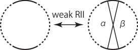
   Figure 10. Weak RI​I on chord diagrams.

   • $\otimes$. Let $\alpha$ and $\beta$ be chords specified in Fig. 10. If $\otimes$ consists of $\alpha$ (resp., $\beta$) and the other chord $e$ is not $\beta$ (resp., $\alpha$), there exists another $\otimes$ consisting of $\beta$ (resp., $\alpha$) and $e$ (the argument of the duality $(\alpha,\beta)$). The number of the sub-chord $\otimes$ consisting of $\alpha$ and $\beta$ is one. Then, $\Delta ch(\otimes)$ is odd. Moreover, $\Delta ch(\otimes)=2(2m-1)+1$ $=$ $4m-1~{}(m\in\mathbb{Z}_{\geq 1})$ by the argument regarding Figs. 8 and 9.

   • . We split the cases by how many increased chords belong to the new from the left to the right in Fig.  10.

     • (one chord in the new.) By the duality $(\alpha,\beta)$, the contribution to the difference is an even number of chords.

     • (two chords in the new.) The number of chords such as $A$ shown in Fig. 11 is odd by the argument regarding Figs. 8 and 9 (cf., case $\otimes$ of strong RI​I).

       

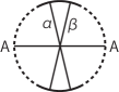
       Figure 11. Appearance of chord $A$ on the right of Fig. 10 under weak RI​I.

   • . There is no possibility that both $\alpha$ and $\beta$ are contained in the new from the left to the right in Fig. 10. Then we consider the duality $(\alpha,\beta)$, which implies $\Delta ch(\begin{picture}(10.0,5.0)\put(5.0,3.0){\circle{7.0}} \qbezier(1.5,3.0)(5.0,3.0)(8.5,3.0)\qbezier(4.0,0.0)(4.0,3.0)(4.0,6.0)\qbezier(6.0,0.0)(6.0,3.0)(6.0,6.0)\end{picture})=$ even.

   • . This case is very similar to the above case, $\Delta ch(\begin{picture}(10.0,5.0)\put(5.0,3.0){\circle{7.0}} \qbezier(1.5,3.0)(5.0,3.0)(8.5,3.0)\qbezier(3.0,0.0)(3.0,3.0)(3.0,5.5)\qbezier(5.0,-0.5)(5.0,3.0)(5.0,6.5)\qbezier(7.0,0.0)(7.0,3.0)(7.0,5.5)\end{picture})=$ even.

4. Strong RI​I​I (Fig. 12). Consider the fourth column of the table in Fig. 4.

   

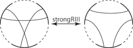
   Figure 12. Strong RI​I​I on chord diagrams.

   • $\otimes$. Fig. 12 directly implies $\Delta ch(\otimes)=\pm 3$ (as in [3]).

   • . We split the cases by the number of chords that relate to the strong RI​I​I and belong to the new from right to left in Fig. 12.

     • (one chord related to the new). By Fig. 12, $\Delta ch(\begin{picture}(10.0,5.0)\put(5.0,3.0){\circle{7.0}} \qbezier(5.0,0.0)(5.0,3.0)(5.0,6.0)\qbezier(2.0,1.0)(5.0,3.0)(8.0,5.0)\qbezier(8.0,1.0)(5.0,3.0)(2.0,5.0)\end{picture})=0$ in this case.

     • (two chords related to the new). In this case, for each chord $X$ shown in Fig. 13, the difference is one from left to right in Fig. 13 (using symmetry, it is sufficient to consider Fig. 13).

       

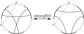
       Figure 13. Chord $X$ appearing in strong RI​I​I.

       We show that the number of such $X$ is even, as follows. First, we apply the same argument as for Figs. 8 and 9 to the leftmost figure of Fig. 3. The operation illustrated in Fig. 14 is useful for showing this.

       

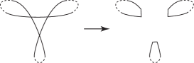
       Figure 14. Resolutions of three double points.

       After the operation illustrated in Fig. 14, two of three components intersect at even double points, which implies the number of chords such as $X$ is even. Since each $X$ produces the difference $\pm 1$, the difference is even in this case.

     • (three chords related to the new). Only one belongs to the new .

     As a result, $\Delta ch(\begin{picture}(10.0,5.0)\put(5.0,3.0){\circle{7.0}} \qbezier(5.0,0.0)(5.0,3.0)(5.0,6.0)\qbezier(2.0,1.0)(5.0,3.0)(8.0,5.0)\qbezier(8.0,1.0)(5.0,3.0)(2.0,5.0)\end{picture})=$ odd.

   • . We separate the cases based on the number of chords, in , that related to the difference between the left and the right of Fig. 12.

     • (one chord related to the difference) By Fig. 12, $\Delta ch(\begin{picture}(10.0,5.0)\put(5.0,3.0){\circle{7.0}} \qbezier(1.5,3.0)(5.0,3.0)(8.5,3.0)\qbezier(4.0,0.0)(4.0,3.0)(4.0,6.0)\qbezier(6.0,0.0)(6.0,3.0)(6.0,6.0)\end{picture})=0$.

     • (two chords related to the difference) The discussion is very similar to the case of . Consider Fig. 13. For each $X$, the difference in the number of H-chords is $\pm 1$ (from two H-chords (left) to one H-chord (right) in Fig. 13). The number of such $X$ is even by the fact that we showed in the case of . As a result, $\Delta ch(\begin{picture}(10.0,5.0)\put(5.0,3.0){\circle{7.0}} \qbezier(1.5,3.0)(5.0,3.0)(8.5,3.0)\qbezier(4.0,0.0)(4.0,3.0)(4.0,6.0)\qbezier(6.0,0.0)(6.0,3.0)(6.0,6.0)\end{picture})=$ even.

     • (three chords related to the difference) In this case, there is no difference contributing to $\Delta ch(\begin{picture}(10.0,5.0)\put(5.0,3.0){\circle{7.0}} \qbezier(1.5,3.0)(5.0,3.0)(8.5,3.0)\qbezier(4.0,0.0)(4.0,3.0)(4.0,6.0)\qbezier(6.0,0.0)(6.0,3.0)(6.0,6.0)\end{picture})$ and $\Delta ch(\begin{picture}(10.0,5.0)\put(5.0,3.0){\circle{7.0}} \qbezier(1.5,3.0)(5.0,3.0)(8.5,3.0)\qbezier(4.0,0.0)(4.0,3.0)(4.0,6.0)\qbezier(6.0,0.0)(6.0,3.0)(6.0,6.0)\end{picture})=0$.

   • . We divide the cases by how many chords in relate to the difference under one strong RI​I​I.

     • (one chord related to the difference) In this case, the number of $I\!I\!I$-chords does not change under strong RI​I​I.

     • (two chords related to the difference) Consider Fig. 15.

       

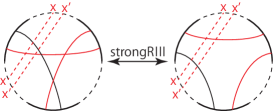
       Figure 15. Appearance of two parallel chords $X$ and $X^{\prime}$ under strong RI​I​I. Two I​I​I-chords, both including $X$ and $X^{\prime}$, are contained on the left hand side.

       As in Fig. 15, the difference in the number of $I\!I\!I$-chords is $\pm 2$ for each pair $(X,X^{\prime})$. Therefore, for all pairs matching $(X,X^{\prime})$, the difference of the sum is even.

       We consider another type of possibility, as shown in Fig. 16.

       

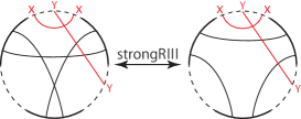
       Figure 16. Appearance of $X$-type and $Y$-type chords under strong RI​I​I. A I​I​I-chord including $X$ and $Y$ is contained on the right hand side.

       For each chord $X$, using Figs. 8 and 9 that is frequently used above, the number of $Y$-type chords shown in Fig. 16 is even. The detailed explanation is as follows. See Fig. 17. First, apply the operation shown in Fig. 14 to the considered diagrams. Second, select the curve $C_{1}$ containing the chord $X$. Third, in the curve $C_{1}$, apply the operation shown in Fig. 9 to the double point corresponding to $X$. Now we have four component curves, of which, two curves intersect at even double points. This is why the number of $Y$-type chords is even.

       

       Figure 17. The number of $Y$-type chords is even.

       Then, for each such $X$, the difference is even. Therefore, the difference of the sum $\Delta ch(\begin{picture}(10.0,5.0)\put(5.0,3.0){\circle{7.0}} \qbezier(1.5,3.0)(5.0,3.0)(8.5,3.0)\qbezier(3.0,0.0)(3.0,3.0)(3.0,5.5)\qbezier(5.0,-0.5)(5.0,3.0)(5.0,6.5)\qbezier(7.0,0.0)(7.0,3.0)(7.0,5.5)\end{picture})$ is even.

     • (three chords related to the difference) There is no possible case.

     As a result, $\Delta ch(\begin{picture}(10.0,5.0)\put(5.0,3.0){\circle{7.0}} \qbezier(1.5,3.0)(5.0,3.0)(8.5,3.0)\qbezier(3.0,0.0)(3.0,3.0)(3.0,5.5)\qbezier(5.0,-0.5)(5.0,3.0)(5.0,6.5)\qbezier(7.0,0.0)(7.0,3.0)(7.0,5.5)\end{picture})=$ even.

5. Weak RI​I​I (Fig. 18). Finally, count the difference in $\Delta ch$ under one weak RI​I​I.

   

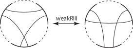
   Figure 18. Weak RI​I​I on chord diagrams.

   • $\otimes$. From Fig. 18, $\Delta ch(\otimes)=\pm 1$.

   • , , and . Since one weak RI​I​I consists of two strong RI​Is and a strong RI​I​I, $\Delta ch(\begin{picture}(10.0,5.0)\put(5.0,3.0){\circle{7.0}} \qbezier(5.0,0.0)(5.0,3.0)(5.0,6.0)\qbezier(2.0,1.0)(5.0,3.0)(8.0,5.0)\qbezier(8.0,1.0)(5.0,3.0)(2.0,5.0)\end{picture})=$ odd, $\Delta ch(\begin{picture}(10.0,5.0)\put(5.0,3.0){\circle{7.0}} \qbezier(1.5,3.0)(5.0,3.0)(8.5,3.0)\qbezier(4.0,0.0)(4.0,3.0)(4.0,6.0)\qbezier(6.0,0.0)(6.0,3.0)(6.0,6.0)\end{picture})=$ even, and $\Delta ch(\begin{picture}(10.0,5.0)\put(5.0,3.0){\circle{7.0}} \qbezier(1.5,3.0)(5.0,3.0)(8.5,3.0)\qbezier(3.0,0.0)(3.0,3.0)(3.0,5.5)\qbezier(5.0,-0.5)(5.0,3.0)(5.0,6.5)\qbezier(7.0,0.0)(7.0,3.0)(7.0,5.5)\end{picture})=$ even.

∎

Remark 1.

[3] contains the results for the first, strong third, and weak third Reidemeister moves on $\otimes$.

Remark 2.

Using Theorem 1, we can easily create some invariants of knot projections in simple ways. Observing the table in Fig. 4, $\otimes(P)\equiv\begin{picture}(10.0,5.0)\put(5.0,3.0){\circle{7.0}} \qbezier(5.0,0.0)(5.0,3.0)(5.0,6.0)\qbezier(2.0,1.0)(5.0,3.0)(8.0,5.0)\qbezier(8.0,1.0)(5.0,3.0)(2.0,5.0)\end{picture}(P)$ (mod $2$) and we notice that $\otimes(P)$ (mod $2$), equivalently $\begin{picture}(10.0,5.0)\put(5.0,3.0){\circle{7.0}} \qbezier(5.0,0.0)(5.0,3.0)(5.0,6.0)\qbezier(2.0,1.0)(5.0,3.0)(8.0,5.0)\qbezier(8.0,1.0)(5.0,3.0)(2.0,5.0)\end{picture}(P)$ (mod $2$), is invariant under the first and strong second moves. $\otimes(P)$ (mod $3$) is invariant under the first and strong third moves, introduced in [3]. $\otimes(P)$, $\begin{picture}(10.0,5.0)\put(5.0,3.0){\circle{7.0}} \qbezier(5.0,0.0)(5.0,3.0)(5.0,6.0)\qbezier(2.0,1.0)(5.0,3.0)(8.0,5.0)\qbezier(8.0,1.0)(5.0,3.0)(2.0,5.0)\end{picture}(P)$, $\begin{picture}(10.0,5.0)\put(5.0,3.0){\circle{7.0}} \qbezier(1.5,3.0)(5.0,3.0)(8.5,3.0)\qbezier(4.0,0.0)(4.0,3.0)(4.0,6.0)\qbezier(6.0,0.0)(6.0,3.0)(6.0,6.0)\end{picture}(P)$, and $\begin{picture}(10.0,5.0)\put(5.0,3.0){\circle{7.0}} \qbezier(1.5,3.0)(5.0,3.0)(8.5,3.0)\qbezier(3.0,0.0)(3.0,3.0)(3.0,5.5)\qbezier(5.0,-0.5)(5.0,3.0)(5.0,6.5)\qbezier(7.0,0.0)(7.0,3.0)(7.0,5.5)\end{picture}(P)$ are invariants under the first move.

3. Proof of Theorem 2.

Proof.

To show Theorem 2, we check the difference of

$$3\begin{picture}(10.0,5.0)\put(5.0,3.0){\circle{7.0}} \qbezier(1.5,3.0)(5.0,3.0)(8.5,3.0)\qbezier(4.0,0.0)(4.0,3.0)(4.0,6.0)\qbezier(6.0,0.0)(6.0,3.0)(6.0,6.0)\end{picture}(P)-3\begin{picture}(10.0,5.0)\put(5.0,3.0){\circle{7.0}} \qbezier(5.0,0.0)(5.0,3.0)(5.0,6.0)\qbezier(2.0,1.0)(5.0,3.0)(8.0,5.0)\qbezier(8.0,1.0)(5.0,3.0)(2.0,5.0)\end{picture}(P)+\otimes(P)$$

under Reidemeister moves RI, strong RI​I​I, strong RI​I, weak RI​I, and weak RI​I​I in that order.

• RI. There is no change of $\otimes(P)$ under RI, and then neither $\begin{picture}(10.0,5.0)\put(5.0,3.0){\circle{7.0}} \qbezier(1.5,3.0)(5.0,3.0)(8.5,3.0)\qbezier(4.0,0.0)(4.0,3.0)(4.0,6.0)\qbezier(6.0,0.0)(6.0,3.0)(6.0,6.0)\end{picture}(P)$ nor $\begin{picture}(10.0,5.0)\put(5.0,3.0){\circle{7.0}} \qbezier(5.0,0.0)(5.0,3.0)(5.0,6.0)\qbezier(2.0,1.0)(5.0,3.0)(8.0,5.0)\qbezier(8.0,1.0)(5.0,3.0)(2.0,5.0)\end{picture}(P)$ changes under RI.

• Strong RI​I​I. Consider Fig. 13. Four chords consisting of a dotted chord $X$, called an $X$-type chord, and three other chords, called RI​I​I chords, are depicted explicitly. In addition, recall that the difference in $\otimes(P)$ of a knot projection $P$ under strong RI​I​I is exactly $\pm 3$ supplied by three RI​I​I chords.

  • Difference of contributions by two non-RI​I​I chords and one RI​I​I chord. There are no changes with respect to $\otimes(P)$, $\begin{picture}(10.0,5.0)\put(5.0,3.0){\circle{7.0}} \qbezier(1.5,3.0)(5.0,3.0)(8.5,3.0)\qbezier(4.0,0.0)(4.0,3.0)(4.0,6.0)\qbezier(6.0,0.0)(6.0,3.0)(6.0,6.0)\end{picture}(P)$, and $\begin{picture}(10.0,5.0)\put(5.0,3.0){\circle{7.0}} \qbezier(5.0,0.0)(5.0,3.0)(5.0,6.0)\qbezier(2.0,1.0)(5.0,3.0)(8.0,5.0)\qbezier(8.0,1.0)(5.0,3.0)(2.0,5.0)\end{picture}(P)$, respectively.

  • Difference of contributions by one non-RI​I​I chord and two RI​I​I chords. It is sufficient to consider the difference of contributions by one $X$-type chord and two RI​I​I chords.

    $x$	$x$(left) $-$ $x$(right) in Fig. 13
    $\begin{picture}(10.0,5.0)\put(5.0,3.0){\circle{7.0}} \qbezier(1.5,3.0)(5.0,3.0)(8.5,3.0)\qbezier(4.0,0.0)(4.0,3.0)(4.0,6.0)\qbezier(6.0,0.0)(6.0,3.0)(6.0,6.0)\end{picture}(P)$	$1$
    $\begin{picture}(10.0,5.0)\put(5.0,3.0){\circle{7.0}} \qbezier(5.0,0.0)(5.0,3.0)(5.0,6.0)\qbezier(2.0,1.0)(5.0,3.0)(8.0,5.0)\qbezier(8.0,1.0)(5.0,3.0)(2.0,5.0)\end{picture}(P)$	$1$
    $\otimes(P)$	$0$

    Thus, there is no difference of $3\begin{picture}(10.0,5.0)\put(5.0,3.0){\circle{7.0}} \qbezier(1.5,3.0)(5.0,3.0)(8.5,3.0)\qbezier(4.0,0.0)(4.0,3.0)(4.0,6.0)\qbezier(6.0,0.0)(6.0,3.0)(6.0,6.0)\end{picture}(P)-3\begin{picture}(10.0,5.0)\put(5.0,3.0){\circle{7.0}} \qbezier(5.0,0.0)(5.0,3.0)(5.0,6.0)\qbezier(2.0,1.0)(5.0,3.0)(8.0,5.0)\qbezier(8.0,1.0)(5.0,3.0)(2.0,5.0)\end{picture}(P)+\otimes(P)$ in this case.

  • Difference of contributions by three RI​I​I chords.

    $x$	$x$(left) $-$ $x$(right) in Fig. 13
    $\begin{picture}(10.0,5.0)\put(5.0,3.0){\circle{7.0}} \qbezier(1.5,3.0)(5.0,3.0)(8.5,3.0)\qbezier(4.0,0.0)(4.0,3.0)(4.0,6.0)\qbezier(6.0,0.0)(6.0,3.0)(6.0,6.0)\end{picture}(P)$	$0$
    $\begin{picture}(10.0,5.0)\put(5.0,3.0){\circle{7.0}} \qbezier(5.0,0.0)(5.0,3.0)(5.0,6.0)\qbezier(2.0,1.0)(5.0,3.0)(8.0,5.0)\qbezier(8.0,1.0)(5.0,3.0)(2.0,5.0)\end{picture}(P)$	$1$
    $\otimes(P)$	$3$

    Thus, there is no difference of $3\begin{picture}(10.0,5.0)\put(5.0,3.0){\circle{7.0}} \qbezier(1.5,3.0)(5.0,3.0)(8.5,3.0)\qbezier(4.0,0.0)(4.0,3.0)(4.0,6.0)\qbezier(6.0,0.0)(6.0,3.0)(6.0,6.0)\end{picture}(P)-3\begin{picture}(10.0,5.0)\put(5.0,3.0){\circle{7.0}} \qbezier(5.0,0.0)(5.0,3.0)(5.0,6.0)\qbezier(2.0,1.0)(5.0,3.0)(8.0,5.0)\qbezier(8.0,1.0)(5.0,3.0)(2.0,5.0)\end{picture}(P)+\otimes(P)$ in this case.

• Strong RI​I. Consider Fig. 19.

  

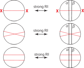
  Figure 19. Dotted chord in the top line: sticking chord $X$, dotted chords in the middle line: a pair of cross chords, dotted chords in the bottom line: a pair of parallel chords.

  • (Top line of Fig. 19) We can assume that the number of chords crossing both $\alpha$ and $\beta$, called sticking chords, is $2m$ ($m\in\mathbb{Z}_{\geq 0}$) by the discussion with respect to Figs. 8 and 9.

    First, we count the difference caused by the tuple, each of which consists of one sticking chord, $\alpha$, and $\beta$.

    $x$	$x$(right)-$x$(left) in Fig. 19
    $\begin{picture}(10.0,5.0)\put(5.0,3.0){\circle{7.0}} \qbezier(1.5,3.0)(5.0,3.0)(8.5,3.0)\qbezier(4.0,0.0)(4.0,3.0)(4.0,6.0)\qbezier(6.0,0.0)(6.0,3.0)(6.0,6.0)\end{picture}(P)$	$2m$
    $\begin{picture}(10.0,5.0)\put(5.0,3.0){\circle{7.0}} \qbezier(5.0,0.0)(5.0,3.0)(5.0,6.0)\qbezier(2.0,1.0)(5.0,3.0)(8.0,5.0)\qbezier(8.0,1.0)(5.0,3.0)(2.0,5.0)\end{picture}(P)$	$0$
    $\otimes(P)$	$4m$

  • (Center line of Fig. 19) Count the difference with respect to tuples, each of which consists of either $\alpha$ or $\beta$ and two sticking chords that mutually intersect and respectively intersect both $\alpha$ and $\beta$ (Fig. 19, the center line). Assume that such $l$ pairs in all the $\binom{2m}{2}$ pairs are types as the center of Fig. 19.

    $x$	$x$(right) $-$ $x$(left) in Fig. 19
    $\begin{picture}(10.0,5.0)\put(5.0,3.0){\circle{7.0}} \qbezier(1.5,3.0)(5.0,3.0)(8.5,3.0)\qbezier(4.0,0.0)(4.0,3.0)(4.0,6.0)\qbezier(6.0,0.0)(6.0,3.0)(6.0,6.0)\end{picture}(P)$	$0$
    $\begin{picture}(10.0,5.0)\put(5.0,3.0){\circle{7.0}} \qbezier(5.0,0.0)(5.0,3.0)(5.0,6.0)\qbezier(2.0,1.0)(5.0,3.0)(8.0,5.0)\qbezier(8.0,1.0)(5.0,3.0)(2.0,5.0)\end{picture}(P)$	$2l$
    $\otimes(P)$	$0$

  • (Bottom line of Fig. 19) Consider $(\binom{2m}{2}-l)$ pairs, as in the bottom line of Fig. 19.

    $x$	$x$(right) $-$ $x$(left) in Fig. 19
    $\begin{picture}(10.0,5.0)\put(5.0,3.0){\circle{7.0}} \qbezier(1.5,3.0)(5.0,3.0)(8.5,3.0)\qbezier(4.0,0.0)(4.0,3.0)(4.0,6.0)\qbezier(6.0,0.0)(6.0,3.0)(6.0,6.0)\end{picture}(P)$	$2(\binom{2m}{2}-l)$
    $\begin{picture}(10.0,5.0)\put(5.0,3.0){\circle{7.0}} \qbezier(5.0,0.0)(5.0,3.0)(5.0,6.0)\qbezier(2.0,1.0)(5.0,3.0)(8.0,5.0)\qbezier(8.0,1.0)(5.0,3.0)(2.0,5.0)\end{picture}(P)$	$0$
    $\otimes(P)$	$0$

  Therefore, the difference is

  $$3\{2(\binom{2m}{2}-l)+2m\}-3\cdot 2l+4m=12m^{2}+4m-12l.$$

• Weak RI​I. Since weak RI​I consists of two RIs, a strong RI​I​I, and three strong RI​Is, the difference of $3\begin{picture}(10.0,5.0)\put(5.0,3.0){\circle{7.0}} \qbezier(1.5,3.0)(5.0,3.0)(8.5,3.0)\qbezier(4.0,0.0)(4.0,3.0)(4.0,6.0)\qbezier(6.0,0.0)(6.0,3.0)(6.0,6.0)\end{picture}(P)$ $-$ $3\begin{picture}(10.0,5.0)\put(5.0,3.0){\circle{7.0}} \qbezier(5.0,0.0)(5.0,3.0)(5.0,6.0)\qbezier(2.0,1.0)(5.0,3.0)(8.0,5.0)\qbezier(8.0,1.0)(5.0,3.0)(2.0,5.0)\end{picture}(P)$ $+$ $\otimes(P)$ is $4n$ ($n\in\mathbb{Z}_{\geq 0}$) under one weak RI​I.

• Weak RI​I​I. Since one weak RI​I​I consists of two strong RI​Is and a strong RI​I​I, the difference of $3\begin{picture}(10.0,5.0)\put(5.0,3.0){\circle{7.0}} \qbezier(1.5,3.0)(5.0,3.0)(8.5,3.0)\qbezier(4.0,0.0)(4.0,3.0)(4.0,6.0)\qbezier(6.0,0.0)(6.0,3.0)(6.0,6.0)\end{picture}(P)-3\begin{picture}(10.0,5.0)\put(5.0,3.0){\circle{7.0}} \qbezier(5.0,0.0)(5.0,3.0)(5.0,6.0)\qbezier(2.0,1.0)(5.0,3.0)(8.0,5.0)\qbezier(8.0,1.0)(5.0,3.0)(2.0,5.0)\end{picture}(P)+\otimes(P)$ is $4n~{}(n\in\mathbb{Z}_{\geq 0})$ under one weak RI​I​I.

Any knot projection $P$ is related to a simple closed curve by a finite sequence consisting of RI, RI​I, and RI​I​I. RI​I (resp., RI​I​I) consists of strong and weak RI​I (resp., RI​I​I). Now we have that each difference of RI, RI​I, and RI​I​I is $4k~{}(k\in\mathbb{Z})$ and $3\begin{picture}(10.0,5.0)\put(5.0,3.0){\circle{7.0}} \qbezier(1.5,3.0)(5.0,3.0)(8.5,3.0)\qbezier(4.0,0.0)(4.0,3.0)(4.0,6.0)\qbezier(6.0,0.0)(6.0,3.0)(6.0,6.0)\end{picture}(\begin{picture}(10.0,5.0)\put(5.0,3.0){\circle{8.0}} \end{picture})-3\begin{picture}(10.0,5.0)\put(5.0,3.0){\circle{7.0}} \qbezier(5.0,0.0)(5.0,3.0)(5.0,6.0)\qbezier(2.0,1.0)(5.0,3.0)(8.0,5.0)\qbezier(8.0,1.0)(5.0,3.0)(2.0,5.0)\end{picture}(\begin{picture}(10.0,5.0)\put(5.0,3.0){\circle{8.0}} \end{picture})+\otimes(\begin{picture}(10.0,5.0)\put(5.0,3.0){\circle{8.0}} \end{picture})=0$. The conditions complete the proof. ∎

4. Proof of Theorem 3 and properties of $\lambda$.

Proof.

First, we recall that $H(P)$, (resp., $\widetilde{X}(P)$) is invariant under RI and strong RI​I​I (resp., weak RI​I​I).

• Invariance of $H(P)$ (cf. [3]). By Theorem 1, $H(P)$ is invariant under RI.

  Now we assume that $H(P)=0$ on the right of Fig. 13. In this case, no $X$-type chord can appear in Fig. 13. Then, no RI​I​I chords can be involved with producing on the right of Fig. 12. If three non-RI​I​I chords comprise in the right chord diagram in Fig. 12, the right chord diagram has , which is contradicts $H(P)=0$. Thus, we notice that $CD_{P}$ has no in the right of Fig. 12 if and only if there is no $X$-type chord and no tuple of three non-RI​I​I chords comprising any . We can also say that $CD_{P}$ has no on the left of Fig. 12 if and only if there is no $X$-type chord and no tuple of three non-RI​I​I chords comprising any . Therefore, when we denote the left (resp., right) knot projection by $P_{l}$ (resp., $P_{r}$) of the arrow of strong RI​I​I in Fig. 3,

  $$H(P_{l})=0\Leftrightarrow H(P_{r})=0.$$

  Thus,

  $$H(P_{l})=1\Leftrightarrow H(P_{r})=1.$$

• Invariance of $\widetilde{X}(P)$. By Theorem 1, $\widetilde{X}(P)$ is invariant under RI. Every chord diagram appearing in Fig. 18 always satisfies $\widetilde{X}(P)=1$.

Second, we recall one of the facts from Sakamoto-Taniyama [5, Theorem 3.2].

Fact 1 (Sakamoto-Taniyama [5]).

Let $P$ be an immersed plane curve. A chord diagram $CD_{P}$ does not contain if and only if $P$ is equivalent to any connected sum of some plane curves, each of which is equivalent to one of the plane curves as , $\infty$, $P_{1}$, $P_{2}$, $P_{3}$, …as illustrated in Fig. 20.

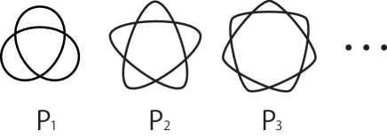
Figure 20. $(2,2i+1)$-torus knot projection $P_{i}$.

Notice that the same claim holds for knot projections with any possible choice of exterior region.

$$H(P)=0\Leftrightarrow P~{}{\text{is any connected sum of knot projections, each of which is}}$$

$${\text{an element of}}~{}\mathcal{T}=\{\begin{picture}(10.0,5.0)\put(5.0,3.0){\circle{8.0}} \end{picture},\infty,{P_{i}}~{}(1\leq i\in\mathbb{Z})\}.$$

Now, we prove the first formula of Theorem 3. Assume that $H(P)=0$ and $\lambda(P)=0$. In this case, it is sufficient to consider any connected sum of elements in $\mathcal{T}$. Note that $\lambda(P\sharp P^{\prime})$ $=$ $\lambda(P)$ $+$ $\lambda(P^{\prime})$, where $P\sharp P^{\prime}$ is the connected sum of $P$ and $P^{\prime}$. Thus $\lambda(P)<0$ if $P$ is a connected sum of knot projections satisfying $H(P)=0$ and at least one member is $P_{2i+1}~{}(i>1)$. This is because $\lambda(\begin{picture}(10.0,5.0)\put(5.0,3.0){\circle{8.0}} \end{picture})=\lambda(\infty)=0$ and $4\lambda(P_{2i+1})$ $=$ $-3\begin{picture}(10.0,5.0)\put(5.0,3.0){\circle{7.0}} \qbezier(5.0,0.0)(5.0,3.0)(5.0,6.0)\qbezier(2.0,1.0)(5.0,3.0)(8.0,5.0)\qbezier(8.0,1.0)(5.0,3.0)(2.0,5.0)\end{picture}(P_{2i+1})+\otimes(P_{2i+1})$ $=$ $-3\binom{2i+1}{3}$ $+$ $\binom{2i+1}{2}$ $=$ $i(2i+1)(1-i)$. Then, if $H(P)=\lambda(P)=0$, $P$ is a connected sum of knot projections, each of which is an element of ${\mathcal{T}}_{1}$ $=$ $\{\begin{picture}(10.0,5.0)\put(5.0,3.0){\circle{8.0}} \end{picture},\infty,P_{1}\}$. Therefore, $P$ can be related to a simple closed curve by a finite sequence consisting of RI and strong RI​I​I.

Conversely, if $P$ can be related to a simple closed curve by a finite sequence consisting of RI and strong RI​I​I, then $H(P)=\lambda(P)=0$.

Then, we have

$$H(P)=\lambda(P)=0\Leftrightarrow P~{}{\text{can be related to $\begin{picture}(10.0,5.0)\put(5.0,3.0){\circle{8.0}} \end{picture}$ by using $RI$ and strong RI\!I\!I}.}$$

This completes the proof of the first formula of Theorem 3.

Next, we show the fourth formula before considering the second and third formulae. Assume that $\widetilde{X}(P)=0$. In this case, we have a chord diagram with no chord intersections. A knot projection $P$ having such a chord diagram can be related to a simple closed curve by a finite sequence consisting of RI. Conversely, if a knot projection $P$ can be related to by a finite sequence consisting of RI, we have $\otimes(P)=0$, which implies $\widetilde{X}(P)=0$. Then, we have the fourth formula

$$\widetilde{X}(P)=0\Leftrightarrow P~{}{\text{can be related to $\begin{picture}(10.0,5.0)\put(5.0,3.0){\circle{8.0}} \end{picture}$ by using $RI$}.}$$

Now, we consider the third formula. Since $\widetilde{X}(P)$ is invariant under RI and weak RI​I​I,

$$P~{}{\text{can be related to $\begin{picture}(10.0,5.0)\put(5.0,3.0){\circle{8.0}} \end{picture}$ by using $RI$ and weak $RI\!I\!I$}}\Rightarrow\widetilde{X}(P)=\widetilde{X}(\begin{picture}(10.0,5.0)\put(5.0,3.0){\circle{8.0}} \end{picture})=0.$$

Then

$$\widetilde{X}(P)=0\Leftrightarrow P~{}{\text{can be related to $\begin{picture}(10.0,5.0)\put(5.0,3.0){\circle{8.0}} \end{picture}$ by using $RI$ and weak $RI\!I\!I$}}$$

where we used the fourth formula to show ($\Rightarrow$).

Finally, we show the second formula. We assume that $\begin{picture}(10.0,5.0)\put(5.0,3.0){\circle{7.0}} \qbezier(5.0,0.0)(5.0,3.0)(5.0,6.0)\qbezier(2.0,1.0)(5.0,3.0)(8.0,5.0)\qbezier(8.0,1.0)(5.0,3.0)(2.0,5.0)\end{picture}(P)=\lambda(P)=0$. This condition implies $0$ $=$ $4\lambda(P)$ $=$ $3\begin{picture}(10.0,5.0)\put(5.0,3.0){\circle{7.0}} \qbezier(1.5,3.0)(5.0,3.0)(8.5,3.0)\qbezier(4.0,0.0)(4.0,3.0)(4.0,6.0)\qbezier(6.0,0.0)(6.0,3.0)(6.0,6.0)\end{picture}(P)$ $+$ $\otimes(P)$ and, originally, we have $\begin{picture}(10.0,5.0)\put(5.0,3.0){\circle{7.0}} \qbezier(1.5,3.0)(5.0,3.0)(8.5,3.0)\qbezier(4.0,0.0)(4.0,3.0)(4.0,6.0)\qbezier(6.0,0.0)(6.0,3.0)(6.0,6.0)\end{picture}(P)\geq 0$ and $\otimes(P)\geq 0$. Then $\otimes(P)=\begin{picture}(10.0,5.0)\put(5.0,3.0){\circle{7.0}} \qbezier(1.5,3.0)(5.0,3.0)(8.5,3.0)\qbezier(4.0,0.0)(4.0,3.0)(4.0,6.0)\qbezier(6.0,0.0)(6.0,3.0)(6.0,6.0)\end{picture}(P)=0$. We notice that $\otimes(P)=0$ if and only if $\widetilde{X}(P)=0$, which implies $\begin{picture}(10.0,5.0)\put(5.0,3.0){\circle{7.0}} \qbezier(1.5,3.0)(5.0,3.0)(8.5,3.0)\qbezier(4.0,0.0)(4.0,3.0)(4.0,6.0)\qbezier(6.0,0.0)(6.0,3.0)(6.0,6.0)\end{picture}(P)=0$. Then,

$$\begin{picture}(10.0,5.0)\put(5.0,3.0){\circle{7.0}} \qbezier(5.0,0.0)(5.0,3.0)(5.0,6.0)\qbezier(2.0,1.0)(5.0,3.0)(8.0,5.0)\qbezier(8.0,1.0)(5.0,3.0)(2.0,5.0)\end{picture}(P)=\lambda(P)=0\Leftrightarrow\otimes(P)=\begin{picture}(10.0,5.0)\put(5.0,3.0){\circle{7.0}} \qbezier(1.5,3.0)(5.0,3.0)(8.5,3.0)\qbezier(4.0,0.0)(4.0,3.0)(4.0,6.0)\qbezier(6.0,0.0)(6.0,3.0)(6.0,6.0)\end{picture}(P)=\lambda(P)=0\Leftrightarrow\otimes(P)=0\Leftrightarrow\widetilde{X}(P)=0.$$

Using the proof of the third formula in the above,

$$\begin{picture}(10.0,5.0)\put(5.0,3.0){\circle{7.0}} \qbezier(5.0,0.0)(5.0,3.0)(5.0,6.0)\qbezier(2.0,1.0)(5.0,3.0)(8.0,5.0)\qbezier(8.0,1.0)(5.0,3.0)(2.0,5.0)\end{picture}(P)=\lambda(P)=0\Leftrightarrow P~{}{\text{can be related to $\begin{picture}(10.0,5.0)\put(5.0,3.0){\circle{8.0}} \end{picture}$ by using $RI$.}}$$

That completes the proof. ∎

The third and fourth formulae in Theorem 3 imply [1, Corollary 4.1].

Corollary 2 ([1]).

A knot projection $P$ can be related to by a finite sequence consisting of RI and weak RI​I​I if and only if $P$ can be related to by a finite sequence consisting of RI.

Remark 3.

The above proof of the first formula in Theorem 3 implies Fact 2 from [3].

Fact 2 (Ito-Takimura-Taniyama [3]).

The following $(\ref{1})$ and $(\ref{2})$ are mutually equivalent.

1. A knot projection $P$ is any connected sum of knot projections, each of which is an element of $\mathcal{T}_{1}$.

2. A knot projection $P$ and a simple closed curve on the sphere can be related by a finite sequence consisting of RI and strong RI​I​I.

As in the proof of Theorem 3, we have

Proposition 1.

Let $P$ and $P^{\prime}$ be arbitrary knot projections and $P\sharp P^{\prime}$ the connected sum of $P$ and $P^{\prime}$. Let $x(P)$ be the number of sub-chord diagrams of type $x$ embedded into $CD_{P}$ for a knot projection $P$, where $x$ does not contain a chord that does not intersect any other chords.

$$x(P\sharp P^{\prime})=x(P)+x(P^{\prime}).$$

As a corollary,

$$\lambda(P\sharp P^{\prime})=\lambda(P)+\lambda(P^{\prime}).$$

Proof.

By the definitions of a chord diagram of a knot projection and $x$, we immediately have $x(P\sharp P^{\prime})=x(P)+x(P^{\prime})$, since chords from $CD_{P}$ and those of $CD_{P^{\prime}}$ do not intersect. In particular, we consider the cases $x=\otimes,\begin{picture}(10.0,5.0)\put(5.0,3.0){\circle{7.0}} \qbezier(5.0,0.0)(5.0,3.0)(5.0,6.0)\qbezier(2.0,1.0)(5.0,3.0)(8.0,5.0)\qbezier(8.0,1.0)(5.0,3.0)(2.0,5.0)\end{picture},\begin{picture}(10.0,5.0)\put(5.0,3.0){\circle{7.0}} \qbezier(1.5,3.0)(5.0,3.0)(8.5,3.0)\qbezier(4.0,0.0)(4.0,3.0)(4.0,6.0)\qbezier(6.0,0.0)(6.0,3.0)(6.0,6.0)\end{picture}$. Then,

$$\lambda(P\sharp P^{\prime}) =\frac{3}{4}\begin{picture}(10.0,5.0)\put(5.0,3.0){\circle{7.0}} \qbezier(1.5,3.0)(5.0,3.0)(8.5,3.0)\qbezier(4.0,0.0)(4.0,3.0)(4.0,6.0)\qbezier(6.0,0.0)(6.0,3.0)(6.0,6.0)\end{picture}(P\sharp P^{\prime})-\frac{3}{4}\begin{picture}(10.0,5.0)\put(5.0,3.0){\circle{7.0}} \qbezier(5.0,0.0)(5.0,3.0)(5.0,6.0)\qbezier(2.0,1.0)(5.0,3.0)(8.0,5.0)\qbezier(8.0,1.0)(5.0,3.0)(2.0,5.0)\end{picture}(P\sharp P^{\prime})+\frac{1}{4}\otimes(P\sharp P^{\prime})$$

$$=\frac{3}{4}\begin{picture}(10.0,5.0)\put(5.0,3.0){\circle{7.0}} \qbezier(1.5,3.0)(5.0,3.0)(8.5,3.0)\qbezier(4.0,0.0)(4.0,3.0)(4.0,6.0)\qbezier(6.0,0.0)(6.0,3.0)(6.0,6.0)\end{picture}(P)+\frac{3}{4}\begin{picture}(10.0,5.0)\put(5.0,3.0){\circle{7.0}} \qbezier(1.5,3.0)(5.0,3.0)(8.5,3.0)\qbezier(4.0,0.0)(4.0,3.0)(4.0,6.0)\qbezier(6.0,0.0)(6.0,3.0)(6.0,6.0)\end{picture}(P^{\prime})-\frac{3}{4}\begin{picture}(10.0,5.0)\put(5.0,3.0){\circle{7.0}} \qbezier(5.0,0.0)(5.0,3.0)(5.0,6.0)\qbezier(2.0,1.0)(5.0,3.0)(8.0,5.0)\qbezier(8.0,1.0)(5.0,3.0)(2.0,5.0)\end{picture}(P)-\frac{3}{4}\begin{picture}(10.0,5.0)\put(5.0,3.0){\circle{7.0}} \qbezier(5.0,0.0)(5.0,3.0)(5.0,6.0)\qbezier(2.0,1.0)(5.0,3.0)(8.0,5.0)\qbezier(8.0,1.0)(5.0,3.0)(2.0,5.0)\end{picture}(P^{\prime})+\frac{1}{4}\otimes(P)+\frac{1}{4}\otimes(P^{\prime})$$

$$=\lambda(P)+\lambda(P^{\prime}).$$

∎

Proposition 2.

For any integer $k$, there exists a knot projection $P$ such that $\lambda(P)=k$.

Proof.

In this proof, we use the symbol as $n_{m}$ to represent a knot projection defined by Figs. 22 and 23. Note that

$$\lambda(4_{1})=4,\lambda(5_{1})=-5,~{}{\text{and}}~{}\lambda(7_{3})=-3.$$

Using the above additivity, $\lambda(4_{1}\sharp 5_{1})=-1$ and $\lambda(4_{1}\sharp 7_{3})=1$. If $k$ is a positive integer, a connected sum $P$ of $k$ pairs, each of which consists of $4_{1}$ and $7_{3}$ satisfies $\lambda(P)=k$. If $k$ is a negative integer, a connected sum $P^{\prime}$ of $k$ pairs, each of which consists of $4_{1}$ and $5_{1}$ satisfies $\lambda(P^{\prime})=k$. Noting that $\lambda(3_{1})=0$, the proof is completed. ∎

5. Proof of Theorem 4.

Proof.

We consider all possibilities of connections of tangles shown in Fig. 5 having four end points. Then, we have exactly six cases (Fig. 21). It is easy to see that we can omit Cases 2, 4, and 6. Moreover, by retaking the shaded part, Case 3 becomes Case 5, and thus, we can omit Case 3. Therefore, in the following, we only consider Cases 1 and 5. Throughout this proof, the phrase shaded parts refers to the shaded parts in Cases 1 and 5 in Fig. 21.

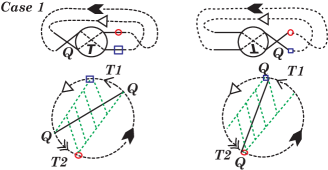
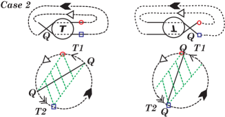
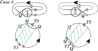
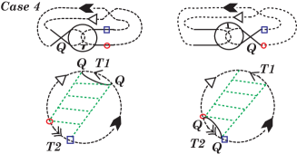
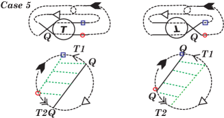
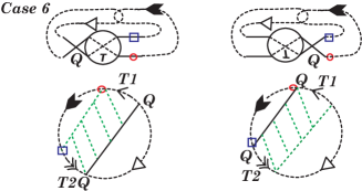
Figure 21. Cases 1–6.

According to the definition of flypes, there is no chord connecting an endpoint on the shaded part with another endpoint on the non-shaded part ($\star$). This condition is called condition $(\star)$. Please refer to the following on the basis of Cases 1 and 5 in Fig. 21. Further, note that we can omit the case wherein $Q$ is not contained by the sub-chord that is being counted, since such a sub-chord should be counted in both before and after applying a flype ($\diamondsuit$).

• $\otimes$.

  • Assume that no chord of $\otimes$ is in the shaded part (zero-chord case). Chord $Q$ is in the shaded part, and therefore, we can omit the case (cf. ($\diamondsuit$)).

  • Assume that exactly one chord of $\otimes$ is in the shaded part (one-chord case). Fig. 21 (Cases 1 and 5) illustrates the claim.

  • Assume that two chords of $\otimes$ are in the shaded part (two-chord case). It is easy to verify the claim in Case 1. Further, note that Case 5 is a case that is not related to $Q$ (cf. ($\diamondsuit$)).

• . We present a discussion similar to that of $\otimes$ case. In the rest of this proof, in the case that $y$ chords of the sub-chord we have chosen (now we choose ) are included in the shaded part in the whole chord diagram, we call the case a “$y$-chord case.”

  • Zero-chord case. The we focus on is not contained in the shaded part and the case is not related to $Q$. Therefore, we can omit the case.

  • One-chord case. Fig. 21 (Cases 1 and 5) illustrates the claim.

  • Two-chord case. Case 5 has no possibility to realize containing $Q$. Fig. 21 (Case 1) illustrates the claim.

  • Three-chord case. Case 5 has no possibility to realize containing $Q$. Case 1 fixes the type of the two other chords crossing $Q$ and we therefore show the claim easily.

  We know that we need not mention the zero-chord case since the case has no possibility to realize the focused sub-chord containing $Q$. Therefore, we omit the zero-chord case in the following.

• . is composed of two parallel chords and the chord crossing the two parallel chords, called the sticking chord.

  • One-chord case. Fig. 21 (Cases 1 and 5) illustrates the claim. In each case, chord $Q$ can either be the sticking chord or a non-sticking chord.

  • Two-chord case. Condition ($\star$) and the case begin considered require that there be no possibility realizing containing $Q$ in Case 1; then, we do not need to consider the case. In Case 5, $Q$ cannot be the sticking chord; it is easy to verify the claim.

  • Three-chord case. Case 5 has no possibility to realize containing $Q$. Case 1 fixes containing $Q$, which becomes the sticking chord, and therefore, we easily obtain the claim.

• .

  • One-chord case. Through Fig. 21 (Cases 1 and 5), it is easy to verify the claim.

  • Two-chords case. We notice that the shaded part must contain two adjacent chords of by the condition ($\star$). Accordingly, there is no possibility to realize containing $Q$ in Case 1. Simlarly, we have the claim in this case using Fig. 21 (Case 5).

  • Three-chord case. Case 1 has no possibility to realize containing $Q$. Case 5 has three parallel chords containing $Q$ in the shaded part and it is easy to verify the claim.

  • Four-chord case. Case 5 has no possibility to realize containing $Q$. In Case 1, $Q$ must cross three parallel chords that fix , and thus, we have the claim.

• .

  • One-chord case. Fig. 21 (Cases 1 and 5) illustrates the claim.

  • Two-chord case. In this case, two parallel strands of must be in the shaded part. Then, Case 1 has no possibility to realize containing $Q$. In Case 5, the claim is easily shown.

  • Three-chord case and Four-chord case. Condition ($\star$) requires that there be no possibility to realize containing $Q$ in Cases 1 and 5.

∎

Remark 4.

In Fig. 24, there are three pairs $(7_{A},7_{6})$, $(7_{B},7_{7})$, and $(7_{C},7_{5})$ with respect to flypes. In each pair, one can be related to another by one flype.

6. Relationship of the number of sub-chord diagrams and Arnold invariants.

This section contains comments regarding the relationship between our study and Arnold invariants. Theorem 1 counts the number of sub-chord diagrams in $CD_{P}$ of a knot projection $P$. In comparison, for the Arnold invariants $J^{+}$, $J^{-}$, and $St$, Averaged invariant $-(J^{+}+2St)/2$ counts the sum of signs $\pm 1$, where each sign is assigned to a sub-chord $\otimes$ (further details can be found in [4]; note also that Polyak’s original Averaged invariant is $(J^{+}+2St)/8$). Let $P$ be an arbitrary knot projection (the image of an immersion) on $S^{2}$. Putting $\infty$ on this arbitrarily selected region $r(\infty)$ from $S^{2}\setminus P$, $P$ can be regard as a plane immersed curve and is denoted by $P_{r}(\infty)$. Arnold invariants, $J^{+}$, $J^{-}$, and $St$, are defined for plane immersed curves. Proceeding further, $J^{+}(P_{r}(\infty)+2St(P_{r(\infty)}))$ does not depend on the selection of $r(\infty)$ (see [4, Sec. 2.4]). Thus, we have an integer $J^{+}(P)+2St(P)$ for an arbitrary spherical curve $P$. Then, Averaged invariant $a(P)$ is defined by

$$a(P)=-(J^{+}(P)+2St(P))/2.$$

Recall that any two knot projections $P_{1}$ and $P_{2}$ are related by a finite sequence of three types of Reidemeister moves, as shown in Fig. 1. The definition of $a(P)$ implies (1)–(5).

Remark 5.

Let $m$ be the total number of weak second and third Reidemeister moves in a finite sequence consisting of first, second, and third Reidemeister moves between two knot projections $P_{1}$ and $P_{2}$.

1. $a(P_{1})-a(P_{2})$ $\equiv$ $m$ (mod $2$) ,

2. $a(P)$ is invariant under RI,

3. $a(P)$ is invariant under strong RI​I

4. a single RI​I​I changes $a(P)$ by $\pm 1$,

5. a single weak RI​I changes $a(P)$ by $\pm 1$.

Proof.

The definitions of $J^{+}$ and $St$ immediately imply (3), (4), and (5). Thus, if we have (2), then we have (1). Here, we recall Polyak’s formula for $a(P)$, which directly implies (2).

Let $X^{*}$ be a $\otimes$ with a base point on $S^{1}$ of $\otimes$ apart from any endpoints of the two chords. Similarly, a chord diagram with a base point is denoted by $CD^{*}_{P}$ which is defined as a chord diagram $CD_{P}$ with a point on $S^{1}$ except for any endpoints of chords. Note that the orientation of $P$ having the base point, which is on the curve except for double points, corresponds to the orientation of $CD^{*}_{P}$ when we always orient $S^{1}$ of $CD_{P}$ counterclockwise. Along the lines of [4, Sec. 6.4], we recall Polyak’s formulation of $a(P)$ as follows.

Let us obtain any orientation of $S^{2}$ and any orientation of a knot projection $P$. We start from the base point and move along the orientation $P$. Each time we pass through a double point for the first time, we attach a sign ($=-1,1$). For each double point through which branch $t$ passes, we assign a pair $(t_{1},t_{2})$ that indicates the orientation rotating from $t_{1}$ to $t_{2}$. If the orientation $(t_{1},t_{2})$ is (resp., is not) equal to the orientation $S^{2}$, the sign of the double point is $-1$ (resp., $1$). For instance, choosing appropriate orientations of the sphere, we describe the sign simply as follows. For each double point having branches $t_{1}$ and $t_{2}$, where $t_{1}$ (resp., $t_{2}$) is the branch we pass through when we pass through the double point for the first (resp., second) time, if $t_{1}$ is the arrow from the bottom left to the top right, the double point has sign $=$ $-1$ and if not, the sign is $1$. Assign each sign of a double point to each corresponding chord. Then sub-chord $X^{*}$ embedded into $CD^{*}_{P}$ has two signs $\epsilon_{0}(X^{*})$ and $\epsilon_{1}(X^{*})$ for each $X^{*}$. As in [4, Page 997, Formula (3)], we can show

$$\sum_{X^{*}~{}{\text{embedded in $CD^{*}_{P}$}}}\epsilon_{0}(X^{*})\epsilon_{1}(X^{*})=a(P).$$

By the above formula, the first Reidemeister move does not affect $a(P)$. That completes the proof. ∎

Remark 6.

We present a table of the values of Averaged invariants $a(P)$ $=$ $-(J^{+}(P)+2St(P))/2$ for prime reduced knot projections with up to seven double points, which appear in Figs. 22 and 23.

​​	$3_{1}$	$4_{1}$	$5_{1}$	$5_{2}$	$6_{1}$	$6_{2}$	$6_{3}$	$7_{1}$	$7_{2}$	$7_{3}$	$7_{4}$	$7_{5}$	$7_{6}$	$7_{7}$	$7_{A}$	$7_{B}$	$7_{C}$
$0$	$-1$	$0$	$-2$	$-1$	$0$	$-1$	$-2$	$-3$	$-1$	$-2$	$-1$	$-2$	$-1$	$0$	$-1$	$0$	$-2$

[2] introduced another integer-valued additive invariant and a complete invariant for prime reduced knot projections with up to seven double points except for one pair under an equivalence relation determined by RI and strong RI​I.

7. Tables of knot projections with invariants.

Finally, we present two tables. The first consists of Figs. 22 and 23. The table contains prime reduced knot projections with up to seven double points and their chord diagrams, each of which has the number of cross chords, triple chords, H-chords, -type sub-chord diagrams, or I​I​I-chords embedded in the chord diagram of the knot projection. Fig. 24 shows prime reduced knot projections with integers that are the values of $\lambda$. Note that prime knot projections lacking only the knot projection $\infty$ are prime reduced knot projections. Here, a prime knot projection is defined as a knot projection that cannot be represented as the connected sum of two non-trivial knot projections. The second table consists of prime reduced knot projections with up to seven double points with $\lambda$. For two knot projections $P_{1}$ and $P_{2}$, we connect $P_{1}$ and $P_{2}$ with a line in the table, if $P_{1}$ can be related to $P_{2}$ using RI and strong RI​I​I under the following rule: except for a pair $(7_{B},7_{4})$, every line indicates the existence of a sequence of a finite number of RIs and a strong RI​I​I (Fig. 24).

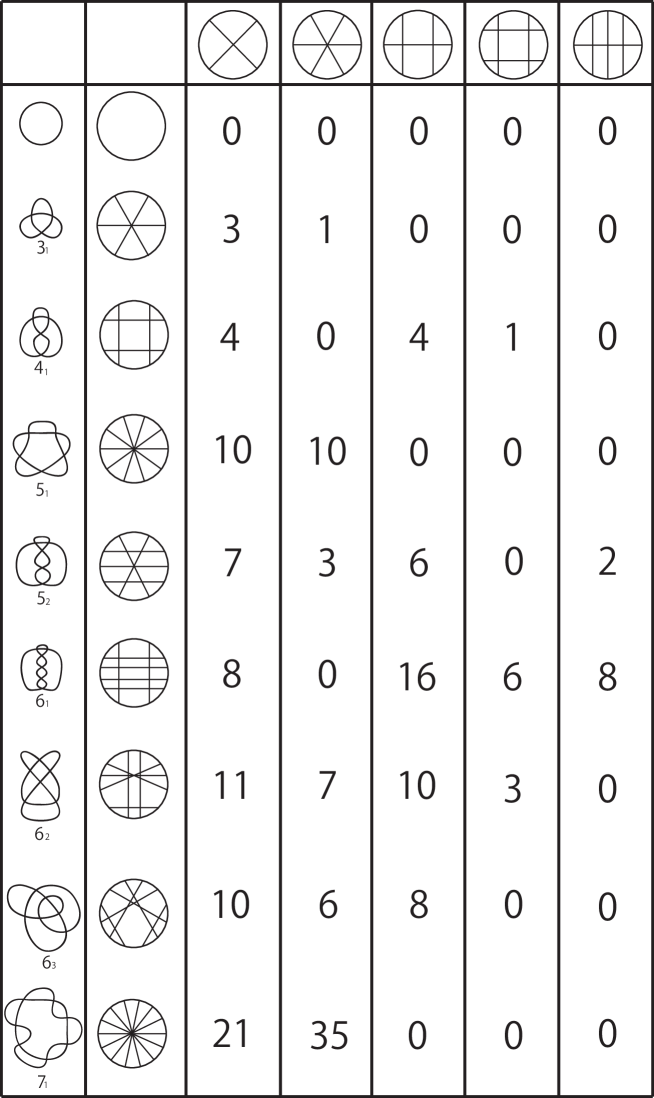
Figure 22. Table 1: knot projections from a simple closed curve to $7_{1}$.

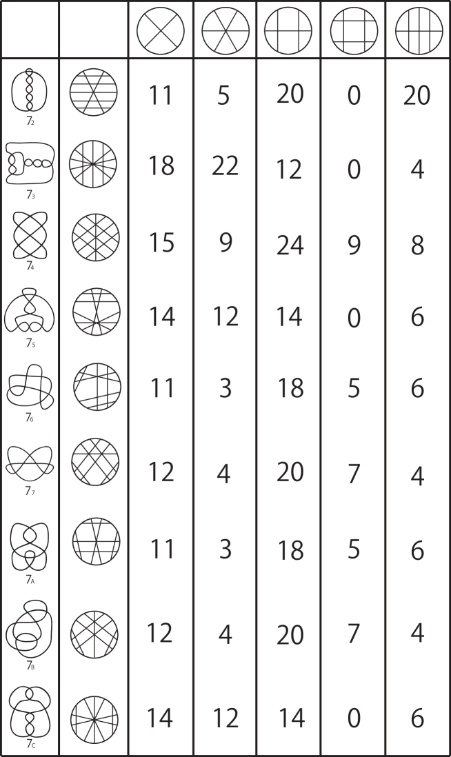
Figure 23. Table 2: knot projections $7_{2}$–$7_{C}$.

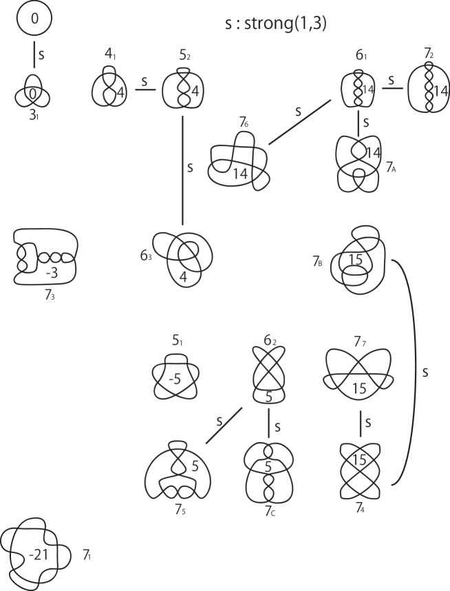
Figure 24. Table of prime reduced knot projections with up to seven double points with $\lambda$. Integers with knot projections stand for $\lambda$.

References

- [1] Ito, N., Takimura, Y.: (1, 2) and weak (1, 3) homotopies on knot projections, J. Knot Theory Ramifications 22 (2013), 1350085 (14 pages).
- [2] Ito, N., Takimura, Y.: Strong and weak (1, 2) homotopies on knot projections and new invariants, to appear in Kobe J. Math.
- [3] Ito, N., Takimura, Y., Taniyama, K.: Strong and weak (1, 3) homotopies on knot projections, to appear in Osaka J. Math.
- [4] Polyak, M.: Invariants of curves and fronts via Gauss diagrams, Topology 37, 989–1009.
- [5] Sakamoto, M., Taniyama, K.: Plane curves in an immersed graph in , J. Knot Theory Ramifications 22 (2013), 1350003, 10pp.