Automatically Eliminating Speculative Leaks from Cryptographic Code with Blade

Extended Version
Marco Vassena CISPA Helmholtz Center for Information SecurityGermany marco.vassena@cispa.saarland Craig Disselkoen UC San DiegoUSA cdisselk@cs.ucsd.edu Klaus von Gleissenthall Vrije Universiteit AmsterdamNetherlands k.freiherrvongleissenthal@vu.nl Sunjay Cauligi UC San DiegoUSA scauligi@eng.ucsd.edu Rami Gökhan Kıcı UC San DiegoUSA rkici@eng.ucsd.edu Ranjit Jhala UC San DiegoUSA jhala@cs.ucsd.edu Dean Tullsen UC San DiegoUSA tullsen@cs.ucsd.edu  and  Deian Stefan UC San DiegoUSA deian@cs.ucsd.edu
(2021)
Abstract.

We introduce Blade, a new approach to automatically and efficiently eliminate speculative leaks from cryptographic code. Blade is built on the insight that to stop leaks via speculative execution, it suffices to cut the dataflow from expressions that speculatively introduce secrets (sources) to those that leak them through the cache (sinks), rather than prohibit speculation altogether. We formalize this insight in a static type system that (1) types each expression as either transient, i.e., possibly containing speculative secrets or as being stable, and (2) prohibits speculative leaks by requiring that all sink expressions are stable. Blade relies on a new abstract primitive, $\mathbf{protect}$, to halt speculation at fine granularity. We formalize and implement $\mathbf{protect}$ using existing architectural mechanisms, and show how Blade’s type system can automatically synthesize a minimal number of $\mathbf{protect}$s to provably eliminate speculative leaks. We implement Blade in the Cranelift WebAssembly compiler and evaluate our approach by repairing several verified, yet vulnerable WebAssembly implementations of cryptographic primitives. We find that Blade can fix existing programs that leak via speculation automatically, without user intervention, and efficiently even when using fences to implement $\mathbf{protect}$.

Speculative execution, Spectre, Constant-time, Type system.
ccs: Security and privacy Formal security modelscopyright: rightsretaineddoi: 10.1145/3434330journalyear: 2021submissionid: popl21main-p403-pjournal: PACMPLjournalvolume: 5journalnumber: POPLarticle: 49publicationmonth: 1

1. Introduction

Implementing secure cryptographic algorithms is hard. The code must not only be functionally correct, memory safe, and efficient, it must also avoid divulging secrets indirectly through side channels like control-flow, memory-access patterns, or execution time. Consequently, much recent work focuses on how to ensure implementations do not leak secrets e.g., via type systems (Cauligi et al., 2019; Watt et al., 2019), verification (Protzenko et al., 2019; Almeida et al., 2016), and program transformations (Barthe et al., 2019).

Unfortunately, these efforts can be foiled by speculative execution. Even if secrets are closely controlled via guards and access checks, the processor can simply ignore these checks when executing speculatively. This, in turn, can be exploited by an attacker to leak protected secrets.

In principle, memory fences block speculation, and hence, offer a way to recover the original security guarantees. In practice, however, fences pose a dilemma. Programmers can restore security by conservatively inserting fences after every load (e.g., using Microsoft’s Visual Studio compiler pass (Donenfeld, 2020)), but at huge performance costs. Alternatively, they can rely on heuristic approaches for inserting fences (Wang et al., 2018), but forgo guarantees about the absence of side-channels. Since missing even one fence can allow an attacker to leak any secret from the address space, secure runtime systems—in particular, browsers like Chrome and Firefox—take yet another approach and isolate secrets from untrusted code in different processes to avoid the risk altogether (Blog, 2010; Mozilla Wiki, 2018). Unfortunately, the engineering effort of such a multi-process redesign is huge—e.g., Chrome’s redesign took five years and roughly 450K lines of code changes (Reis et al., 2019).

In this paper, we introduce Blade, a new, fully automatic approach to provably and efficiently eliminate speculation-based leakage from constant-time cryptographic code. Blade is based on the key insight that to prevent leaking data via speculative execution, it is not necessary to stop all speculation. Instead, it suffices to cut the data flow from expressions (sources) that could speculatively introduce secrets to those that leak them through the cache (sinks). We develop this insight into an automatic enforcement algorithm via four contributions.

A JIT-Step Semantics for Speculation. A key aim of BLADE is to enable source-level reasoning about the absence of speculation-based information leaks. This is crucial to let the source-level type system use control- and data-flow information to optimally prevent leaks. High-level reasoning requires a source-level semantic model of speculation which has, so far, proven to be challenging as the effects of speculation manifest at the very low machine-level: e.g., as branch-prediction affects the streams of low-level instructions that are fetched and (speculatively) executed. We address this challenge with our first contribution: a JIT-step semantics for a high-level While language that lets us reconcile the tension between high-level reasoning and low-level speculation. These semantics translate high-level commands to low-level machine instructions in a just-in-time (JIT) fashion, whilst tracking control-flow predictions at branch points and modeling the speculative execution path of the program as well as the “paths not taken” as stacks of high-level commands.

Our low-level instructions are inspired by a previous formal model of a speculative and out-of-order processor (Cauligi et al., 2020), and let us model the essence of speculation-based attacks—in particular Spectre-PHT (Kocher et al., 2019; Kiriansky and Waldspurger, 2018; Canella et al., 2019)—by modeling precisely how speculation can occur and what an attacker can observe via speculation (§ 3). To prevent leakage, we propose and formalize the semantics of an abstract primitive called $\mathbf{protect}$ that embodies several hardware mechanisms proposed in recent work (Taram et al., 2019; Yu et al., 2019). Crucially, and in contrast to a regular fence which stops all speculation, $\mathbf{protect}$ only stops speculation for a given variable. For example $\mathit{x}\mathbin{:=}\mathbf{protect}(\mathit{e})$ ensures that the value of $e$ is assigned to $x$ only after $e$ has been assigned its stable, non-speculative value. Though we encourage hardware vendors to implement $\mathbf{protect}$ in future processors, for backwards compatibility, we implement and evaluate two versions of $\mathbf{protect}$ on existing hardware—one using fences, another using speculative load hardening (SLH) (Carruth, 2019).

A Type System for Speculation. Our second contribution is an approach to conservatively approximating the dynamic semantics of speculation via a static type sytem that types each expression as either transient (T), i.e., expressions that may contain speculative secrets, or stable (S), i.e., those that cannot (§ 4.1). Our system prohibits speculative leaks by requiring that all sink expressions that can influence intrinsic attacker visible behavior (e.g., cache addresses) are typed as stable. The type system does not rely on user-provided security annotations to identify sensitive sources and public sinks. Instead, we conservatively reject programs that exhibit any flow of information from transient sources to stable sinks. This, in turn, allows us to automatically identify speculative vulnerabilities in existing cryptographic code (where secrets are not explicitly annotated). We connect the static and dynamic semantics by proving that well-typed constant-time programs are secure, i.e., they are also speculative constant-time (Cauligi et al., 2020) (§ 5). This result extends the pre-existing guarantees about sequential constant-time execution of verified cryptographic code to our speculative execution model.

Automatic Protection. Existing programs that are free of $\mathbf{protect}$ statements are likely insecure under speculation (see Section 7 and (Cauligi et al., 2020)) and will be rejected by our type system. Thus, our third contribution is an algorithm that finds potential speculative leaks and automatically synthesizes a minimal number of $\mathbf{protect}$ statements to ensure that the program is speculatively constant-time (§ 4.2). To this end, we extend the type checker to construct a def-use graph that captures the data-flow between program expressions. The presence of a path from transient sources to stable sinks in the graph indicates a potential speculative leak in the program. To repair the program, we only need to identify a cut-set, a set of variables whose removal eliminates all the leaky paths in the graph. We show that inserting a $\mathbf{protect}$ statement for each variable in a cut-set suffices to yield a program that is well-typed, and hence, secure with respect to speculation. Finding such cuts is an instance of the classic Max-Flow/Min-Cut problem, so existing polynomial time algorithms let us efficiently synthesize $\mathbf{protect}$ statements that resolve the dilemma of enforcing security with minimal number of protections.

Blade Tool. Our final contribution is an automatic push-button tool, Blade, which eliminates potential speculative leaks using this min-cut algorithm. Blade extends the Cranelift compiler (Bytecode Alliance, 2020), which compiles WebAssembly (Wasm) to x86 machine code; thus, Blade operates on programs expressed in Wasm. However, operating on Wasm is not fundamental to our approach—we believe that Blade’s techniques can be applied to other programming languages and bytecodes.

We evaluate Blade by repairing verified yet vulnerable (to transient execution attacks) constant-time cryptographic primitives from Constant-time Wasm (CT-Wasm) (Watt et al., 2019) and HACL* (Zinzindohoué et al., 2017) (§ 7). Compared to existing fully automatic speculative mitigation approaches (as notably implemented in Clang), Blade inserts an order of magnitude fewer protections (fences or SLH masks). Blade’s fence-based implementation imposes modest performance overheads: (geometric mean) 5.0% performance overhead on our benchmarks to defend from Spectre v1, or 15.3% overhead to also defend from Spectre v1.1. Both results are significant gains over current solutions. Our fence-free implementation, which automatically inserts SLH masks, is faster in the Spectre v1 case—geometric mean 1.7% overhead—but slower when including Spectre v1.1 protections, imposing 26.6% overhead.

2. Overview

This section gives a brief overview of the kinds of speculative leaks that Blade identifies and how it repairs such programs by careful placement of $\mathbf{protect}$ statements. We then describe how Blade (1) automatically repairs existing programs using our minimal $\mathbf{protect}$ inference algorithm and (2) proves that the repairs are correct using our transient-flow type system.

2.1. Two Kinds of Speculative Leaks

1 void SHA2_update_last(int *input_len, ...)
2 {
3 if (! valid(input_len)) { return; } // Input validation
4 int len = protect(*input_len); // Can speculatively read secret data
5 ...
6 int *dst3 = len + base; // Secret-tainted address
7 ...
8 *dst3 = pad; // Secret-dependent memory access
9 ...
10 for ( i = 0; i < len + ...) // Secret-dependent branch
11 dst2[i] = 0;
12 ...
13 }

Figure 1. Code fragment adapted from the HACL* SHA2 implementation, containing two potential speculative execution vulnerabilities: one through the data cache by writing memory at a secret-tainted address, and one through the instruction cache via a secret-tainted control-flow dependency. The patch computed by Blade is shown in green.

Figure 1 shows a code fragment of the SHA2_update_last function, a core piece of the SHA2 cryptographic hash function implementation, adapted (to simplify exposition) from the HACL* library. This function takes as input a pointer input_len, validates the input (line 3), loads from memory the public length of the hash (line 4, ignore protect for now), calculates a target address dst3 (line 6), and pads the buffer pointed to by dst3 (line 8). Later, it uses len to determine the number of initialization rounds in the condition of the for-loop on line 10.

Leaking Through a Memory Write. During normal, sequential execution this code is not a problem: the function validates the input to prevent classic buffer-overflow vulnerabilities. However, during speculation, an attacker can exploit this function to leak sensitive data. To do this, the attacker first has to mistrain the branch predictor to predict the next input to be valid. Since input_len is a function parameter, the attacker can do this by, e.g., calling the function repeatedly with legitimate addresses. After mistraining the branch predictor this way, the attacker manipulates input_len to point to an address containing secret data and calls the function again, this time with an invalid pointer. As a result of the mistraining, the branch predictor causes the processor to skip validation and load the secret into len, which in turn is used to calculate pointer dst3. The location pointed to by dst3 is then written on line 8, leaking the secret data. Even though pointer dst3 is invalid and the subsequent write will not be visible at the program level (the processor disregards it), the side-effects of the memory access persist in the cache and therefore become visible to the attacker. In particular, the attacker can extract the target address—and thereby the secret—using cache timing measurements (Ge et al., 2018).

Leaking Through a Control-Flow Dependency. The code in Figure 1 contains a second potential speculative vulnerability, which leaks secrets through a control-flow dependency instead of a memory access. To exploit this vulnerability, the attacker can similarly manipulate the pointer input_len to point to a secret after mistraining the branch predictor to skip validation. But instead of leaking the secret directly through the data cache, the attacker can leak the value indirectly through a control-flow dependency: in this case, the secret determines how often the initialization loop (line 10) is executed during speculation. The attacker can then infer the value of the secret from a timing attack on the instruction cache or (much more easily) on iteration-dependent lines of the data cache.

2.2. Eliminating Speculative Leaks

Preventing the Leak using Memory Fences. Since these leaks exploit the fact that input validation is speculatively skipped, we can prevent them by making sure that dangerous operations such as the write on line 8 or the loop condition check on line 10 are not executed until the input has been validated. Intel (2018a), AMD (2018), and others (Pardoe, 2018; Donenfeld, 2020) recommend doing this by inserting a speculation barrier after critical validation check-points. This would place a memory fence after line 3, but anywhere between lines 3 and 8 would work. This fence would stop speculation over the fence: statements after the fence will not be executed until all statements up to the fence (including input validation) executed. While fences can prevent leaks, using fences as such is more restrictive than necessary—they stop speculative execution of all following instructions, not only of the instructions that leak—and thus incur a high performance cost (Tkachenko, 2018; Taram et al., 2019).

Preventing the Leak Efficiently. We do not need to stop all speculation to prevent leaks. Instead, we only need to ensure that potentially secret data, when read speculatively, cannot be leaked. To this end, we propose an alternative way to stop speculation from reaching the operations on line 8 and line 10, through a new primitive called $\mathbf{protect}$. Rather than eliminate all speculation, $\mathbf{protect}$ only stops speculation along a particular data-path. We use $\mathbf{protect}$ to patch the program on line 4. Instead of assigning the value len directly from the result of the load, the memory load is guarded by a $\mathbf{protect}$ statement. This ensures that the value assigned to len is always guaranteed to use the input_len pointer’s final, nonspeculative value. This single $\mathbf{protect}$ statement on line 4 is sufficient to fix both of the speculative leaks described in Section 2.1—it prevents any speculative, secret data from reaching lines 8 or 10 where it could be leaked to the attacker.

Implementation of protect. Our $\mathbf{protect}$ primitive provides an abstract interface for fine grained control of speculation. This allows us to eliminate speculation-based leaks precisely and only when needed. However, whether $\mathbf{protect}$ can eliminate leaks with tolerable runtime overhead depends on its concrete implementation. We consider and formalize two implementations: an ideal implementation and one we can implement on today’s hardware.

To have fine grain control of speculation, $\mathbf{protect}$ must be implemented in hardware and exposed as part of the ISA. Though existing processors provide only coarse grained control over speculation through memory fence instructions, this might change in the future. For example, recently proposed microprocessor designs (Taram et al., 2019; Yu et al., 2019) provide new hardware mechanisms to control speculation, in particular to restrict targeted types of speculation while allowing other speculation to proceed: this suggests that $\mathbf{protect}$ could be implemented efficiently in hardware in the future.

Even if future processors implement $\mathbf{protect}$, we still need to address Spectre attacks on existing hardware. Hence, we formalize and implement $\mathbf{protect}$ in software, building on recent Spectre attack mitigations (Schwarz et al., 2020). Specifically, we propose a self-contained approach inspired by Clang’s Speculative Load Hardening (SLH) (Carruth, 2019). At a high level, Clang’s SLH stalls speculative load instructions in a conditional block by inserting artificial data-dependencies between loaded addresses and the value of the condition. This ensures that the load is not executed before the branch condition is resolved. Unfortunately, this approach unnecessarily stalls all non-constant conditional load instructions, regardless of whether they can influence a subsequent load and thus can actually cause speculative data leaks. Furthermore, this approach is unsound—it can also miss some speculative leaks, e.g., if a load instruction is not in the same conditional block that validates its address (like the code in Figure 1). In contrast to Clang, our approach applies SLH selectively, only to individual load instructions whose result flows to an instruction which might leak, and precisely, by using accurate bounds-check conditions to ensure that only data from valid addresses can be loaded.

2.3. Automatically Repairing Speculative Leaks via $\mathbf{protect}$-Inference

Example
$\mathit{x}\mathbin{:=}\mathit{a}{[}\mathit{i}_{1}{]}$
$\mathit{y}\mathbin{:=}\mathit{a}{[}\mathit{i}_{2}{]}$
$\mathit{z}\mathbin{:=}\mathit{x}\mathbin{+}\mathit{y}$
$\mathit{w}\mathbin{:=}\mathit{b}{[}\mathit{z}{]}$
Example Patched
x:=𝐩𝐫𝐨𝐭𝐞𝐜𝐭(a[i1])assign𝑥𝐩𝐫𝐨𝐭𝐞𝐜𝐭𝑎delimited-[]subscript𝑖1\mathit{x}\mathbin{:=}{\color[rgb]{1,0.49,0}\definecolor[named]{pgfstrokecolor}{rgb}{1,0.49,0}\pgfsys@color@cmyk@stroke{0}{0.51}{1}{0}\pgfsys@color@cmyk@fill{0}{0.51}{1}{0}\mathbf{protect}}(\mathit{a}{[}\mathit{i}_{1}{]})
y:=𝐩𝐫𝐨𝐭𝐞𝐜𝐭(a[i2])assign𝑦𝐩𝐫𝐨𝐭𝐞𝐜𝐭𝑎delimited-[]subscript𝑖2\mathit{y}\mathbin{:=}{\color[rgb]{1,0.49,0}\definecolor[named]{pgfstrokecolor}{rgb}{1,0.49,0}\pgfsys@color@cmyk@stroke{0}{0.51}{1}{0}\pgfsys@color@cmyk@fill{0}{0.51}{1}{0}\mathbf{protect}}(\mathit{a}{[}\mathit{i}_{2}{]})
z:=𝐩𝐫𝐨𝐭𝐞𝐜𝐭(x+y)assign𝑧𝐩𝐫𝐨𝐭𝐞𝐜𝐭𝑥𝑦\mathit{z}\mathbin{:=}{\color[rgb]{0,0.88,0}\definecolor[named]{pgfstrokecolor}{rgb}{0,0.88,0}\pgfsys@color@cmyk@stroke{0.91}{0}{0.88}{0.12}\pgfsys@color@cmyk@fill{0.91}{0}{0.88}{0.12}\mathbf{protect}}(\mathit{x}\mathbin{+}\mathit{y})
$\mathit{w}\mathbin{:=}\mathit{b}{[}\mathit{z}{]}$
Figure 2. Running example. Program Example is shown on the left and the patched program is shown on the right. The orange patch is sub-optimal because it requires more $\mathbf{protect}$ statements than the optimal green patch.

Blade automatically finds potential speculative leaks and synthesizes a minimal number of $\mathbf{protect}$ statements to eliminate the leaks. We illustrate this process using the simple program Example in Figure 2 as a running example. The program reads two values from an array ($\mathit{x}\mathbin{:=}\mathit{a}{[}\mathit{i}_{1}{]}$ and $\mathit{y}\mathbin{:=}\mathit{a}{[}\mathit{i}_{2}{]}$), adds them ($\mathit{z}\mathbin{:=}\mathit{x}\mathbin{+}\mathit{y}$), and indexes another array with the result ($\mathit{w}\mathbin{:=}\mathit{b}{[}\mathit{z}{]}$). This program is written using our formal calculus in which all array operations are implicitly bounds-checked and thus no explicit validation code is needed.

Like the SHA2 example from Figure 1, Example contains a speculative execution vulnerability: the speculative array reads could bypass their bounds checks and so $\mathit{x}$ and $\mathit{y}$ can contain transient secrets (i.e., secrets introduced by misprediction). This secret data then flows to $\mathit{z}$, and finally leaks through the data cache when reading $\mathit{b}{[}\mathit{z}{]}$.

Def-Use Graph.

T$a[i_{2}]$ $a[i_{1}]$ $x$ $y$ $x+y$ $z$S
Figure 3. Subset of the def-use graph of Example. The dashed lines identify two valid choices of cut-sets. The left cut requires removing two nodes and thus inserting two $\mathbf{protect}$ statements. The right cut shows a minimal solution, which only requires removing a single node.

To secure the program, we need to cut the dataflow between the array reads which could introduce transient secret values into the program, and the index in the array read where they are leaked through the cache. For this, we first build a def-use graph whose nodes and directed edges capture the data dependencies between the expressions and variables of a program. For example, consider (a subset of) the def-use graph of program Example in Figure 3. In the graph, the edge $\mathit{x}\to\mathit{x}\mathbin{+}\mathit{y}$ indicates that $\mathit{x}$ is used to compute $\mathit{x}\mathbin{+}\mathit{y}$. To track how transient values propagate in the def-use graph, we extend the graph with the special node T, which represents the source of transient values of the program. Since reading memory creates transient values, we connect the T node to all nodes containing expressions that explicitly read memory, e.g., Ta[i1]T𝑎delimited-[]subscript𝑖1{\color[rgb]{1,0,1}\definecolor[named]{pgfstrokecolor}{rgb}{1,0,1}\pgfsys@color@cmyk@stroke{0}{1}{0}{0}\pgfsys@color@cmyk@fill{0}{1}{0}{0}\textbf{T}}\to\mathit{a}{[}\mathit{i}_{1}{]}. Following the data dependencies along the edges of the def-use graph, we can see that node T is transitively connected to node $\mathit{z}$, which indicates that $\mathit{z}$ can contain transient data at runtime. To detect insecure uses of transient values, we then extend the graph with the special node S, which represents the sink of stable (i.e., non-transient) values of a program. Intuitively, this node draws all the values of a program that must be stable to avoid transient execution attacks. Therefore, we connect all expression used as array indices in the program to the S node, e.g., zS𝑧S\mathit{z}\to{\color[rgb]{0.15,1,0.67}\definecolor[named]{pgfstrokecolor}{rgb}{0.15,1,0.67}\pgfsys@color@cmyk@stroke{0.85}{0}{0.33}{0}\pgfsys@color@cmyk@fill{0.85}{0}{0.33}{0}\textbf{S}}. The fact that the graph in Figure 3 contains a path from T to S indicates that transient data flows through data dependencies into (what should be) a stable index expression and thus the program may be leaky.

Cutting the Dataflow. In order to make the program safe, we need to cut the data-flow between T and S by introducing $\mathbf{protect}$ statements. This problem can be equivalently restated as follows: find a cut-set, i.e., a set of variables, such that removing the variables from the graph eliminates all paths from  T to S. Each choice of cut-set defines a way to repair the program: simply add a $\mathbf{protect}$ statement for each variable in the set. Figure 3 contains two choices of cut-sets, shown as dashed lines. The cut-set on the left requires two protect statements, for variables $x$ and $y$ respectively, corresponding to the orange patch in Figure 2. The cut-set on the right is minimal, it requires only a single protect, for variable $z$, and corresponds to the green patch in Figure 2. Intuitively, minimal cut-sets result in patches that introduce as few $\mathbf{protect}$s as needed and therefore allow more speculation. Luckily, the problem of finding a minimal cut-set is an instance of the classic Min-Cut/Max-Flow problem, which can be solved using efficient, polynomial-time algorithms (Ford and Fulkerson, 2010). For simplicity, Blade adopts a uniform cost model and therefore synthesizes patches that contain a minimal number of $\mathbf{protect}$ statements, regardless of their position in the code and how many times they can be executed. Though our evaluation shows that even this simple model imposes modest overheads (§7), our implementation can be easily optimized by considering additional criteria when searching for a minimal cut set, with further performance gain likely. For example, we could assign weights proportional to execution frequency, or introduce penalties for placing $\mathbf{protect}$ inside loops.

2.4. Proving Correctness via Transient-Flow Types

To ensure that we add $\mathbf{protect}$ statements in all the right places (without formally verifying our repair algorithm), we use a type system to prove that patched programs are secure, i.e., they satisfy a semantic security condition. The type system simplifies the security analysis—we can reason about program execution directly rather than through generic flows of information in the def-use graph. Moreover, restricting the security analysis to the type system makes the security proofs independent of the specific algorithm used to compute the program repairs (e.g., the Max-Flow/Min-Cut algorithm). As long as the repaired program type checks, Blade’s formal guarantees hold. To show that the patches obtained from cutting the def-use graph of a given program are correct (i.e., they make the program well-typed), our transient-flow type system constructs its def-use graph from the type-constraints generated during type inference.

Typing Judgement. Our type system statically assigns a transient-flow type to each variable: a variable is typed as transient (written as T), if it can contain transient data (i.e., potential secrets) at runtime, and as stable (written as S), otherwise. For instance, in program Example (Fig. 3) variables $\mathit{x}$ and $\mathit{y}$ (and hence $\mathit{z}$) are typed as transient because they may temporarily contain secret data originated from speculatively reading the array out of bounds. Given a typing environment $\Gamma$ which assigns a transient-flow type to each variable, and a command $c$, the type system defines a judgement $\Gamma\vdash c$ saying that $c$ is free of speculative execution bugs (§ 4.1). The type system ensures that transient expressions are not used in positions that may leak their value by affecting memory reads and writes, e.g., they may not be used as array indices and in loop conditions. Additionally, it ensures that transient expressions are not written to stable variables, except via $\mathbf{protect}$. For example, our type system rejects program Example because it uses transient variable $\mathit{z}$ as an array index, but it accepts program Example Patched in which $\mathit{z}$ can be typed stable thanks to the $\mathbf{protect}$ statements. We say that variables whose assignment is guarded by a $\mathbf{protect}$ statement (like $\mathit{z}$ in Example Patched) are “protected variables”.

To study the security guarantees of our type system, we define a JIT-step semantics for speculative execution of a high-level While language (§ 3), which resolves the tension between source-level reasoning and machine-level speculation. We then show that our type system indeed prevents speculative execution attacks, i.e., we prove that well-typed programs remain constant-time under the speculative semantics (§ 5).

Type Inference. Given an input program, we construct the corresponding def-use graph by collecting the type constraints generated during type inference. Type inference is formalized by a typing-inference judgment $\Gamma,\mathsf{Prot}\vdash\mathit{c}\Rightarrow\mathit{k}$ (§ 4.2), which extends the typing judgment from above with (1) a set of implicitly protected variables $\mathsf{Prot}$ (the cut-set), and (2) a set of type-constraints $\mathit{k}$ (the def-use graph). Intuitively, the set $\mathsf{Prot}$ identifies the variables of program $\mathit{c}$ that contain transient data and that must be protected (i.e., they must be made stable using $\mathbf{protect}$) to avoid leaks. At a high level, type inference has 3 steps: (i) generate a set of constraints under an initial typing environment and protected set that allow any program to type-check, (ii) construct the def-use graph from the constraints and find a cut-set (the final protected set), and (iii) compute the final typing environment which types the variables in the cut-set as stable. To characterize the security of a still unrepaired program after type inference, we define a typing judgment $\Gamma,\mathsf{Prot}\vdash\mathit{c}$, where unprotected variables are explicitly accounted for in the $\mathsf{Prot}$ set.111The judgment $\Gamma\vdash\mathit{c}$ is just a short-hand for $\Gamma,\varnothing\vdash\mathit{c}$. Intuitively, the program is secure if we promise to insert a $\mathbf{protect}$ statement for each variable in $\mathsf{Prot}$. To repair programs, we simply honor this promise and insert a protect statement for each variable in the protected set of the typing judgment obtained above. Once repaired, the program type checks under an empty protected set.

2.5. Attacker Model

We delineate the extents of the security guarantees of our type system and repair algorithm by discussing the attacker model considered in this work. We assume an attacker model where the attacker runs cryptographic code, written in Wasm, on a speculative out-of-order processor; the attacker can influence how programs are speculatively executed using the branch predictor and choose the instruction execution order in the processor pipeline. The attacker can make predictions based on control-flow history and memory-access patterns similar to real, adaptive predictors. Though these predictions can depend on secret information in general, we assume that they are secret-independent for the constant-time programs repaired by Blade.

We assume that the attacker can observe the effects of their actions on the cache, even if these effects are otherwise invisible at the ISA level. In particular, while programs run, the attacker can take precise timing measurements of the data- and instruction-cache with a cache-line granularity, and thus infer the value of secret data. These features allow the attacker to mount Spectre-PHT attacks (Kocher et al., 2019; Kiriansky and Waldspurger, 2018) and exfiltrate data through FLUSH+RELOAD (Yarom and Falkner, 2014) and PRIME+PROBE (Tromer et al., 2010) cache side-channel attacks. We do not consider speculative attacks that rely on the Return Stack Buffer (e.g., Spectre-RSB (Maisuradze and Rossow, 2018; Koruyeh et al., 2018)), Branch Target Buffer (Spectre-BTB (Kocher et al., 2019)), or Store-to-Load forwarding misprediction (Spectre-STL (Horn, 2018), recently reclassified as a Meltdown attack (Moghimi et al., 2020)). We similarly do not consider Meltdown attacks (Lipp et al., 2018) or attacks that do not use the cache to exfiltrate data, e.g., port contention (SMoTherSpectre (Bhattacharyya et al., 2019)).

3. A JIT-Step Semantics for Speculation

$\displaystyle\text{Values }\mathit{v}$ $\displaystyle\Coloneqq\mathit{n}\;\;|\;\;\mathit{b}\;\;|\;\;\mathit{a}$
$\displaystyle\text{Expr. }\mathit{e}$ $\displaystyle\Coloneqq\mathit{v}\;\;|\;\;\mathit{x}\;\;|\;\;\mathit{e}\mathbin{+}\mathit{e}\;\;|\;\;\mathit{e}<\mathit{e}$
$\displaystyle\ \;|\;\;\mathit{e}\;\otimes\;\mathit{e}\;\;|\;\;\mathit{e}\mathbin{?}\mathit{e}\mathbin{:}\mathit{e}$
$\displaystyle\ \;|\;\;\mathit{length}(\mathit{e})\;\;|\;\;\mathit{base}(\mathit{e})$
$\displaystyle\text{Rhs. }\mathit{r}$ $\displaystyle\Coloneqq\mathit{e}\;\;|\;\;\ast\mathit{e}\;\;|\;\;\mathit{a}{[}\mathit{e}{]}$
$\displaystyle\text{Cmd. }\mathit{c}$ $\displaystyle\Coloneqq\mathbf{skip}\;\;|\;\;\mathit{x}\mathbin{:=}\mathit{r}\;\;|\;\;\ast\mathit{e}\mathrel{=}\mathit{e}$
$\displaystyle\ \;|\;\;\mathit{a}{[}\mathit{e}{]}\mathbin{:=}\mathit{e}\;\;|\;\;\mathbf{fail}\;\;|\;\;\mathit{c};\mathit{c}$
$\displaystyle\ \;|\;\;\mathbf{if}\;\mathit{e}\;\mathbf{then}\;\mathit{c}\;\mathbf{else}\;\mathit{c}$
$\displaystyle\ \;|\;\;\mathbf{while}\;\mathit{e}\;\mathbf{do}\;\mathit{c}$
$\displaystyle\ \;|\;\;\mathit{x}\mathbin{:=}\mathbf{protect}(\mathit{r})$
(a) Source syntax.
$\displaystyle\text{Instructions }\mathit{i}$ $\displaystyle\Coloneqq\mathbf{nop}\;\;|\;\;\mathit{x}\mathbin{:=}\mathit{e}\;\;|\;\;\mathit{x}\mathbin{:=}\mathbf{load}(\mathit{e})$
$\displaystyle\ \;|\;\;\mathbf{store}(\mathit{e},\mathit{e})\;\;|\;\;\mathit{x}\mathbin{:=}\mathbf{protect}(\mathit{e})$
$\displaystyle\ \;|\;\;\mathbf{guard}(\mathit{e}^{\mathit{b}},\mathit{cs},\mathit{p})\;\;|\;\;\mathbf{fail}(\mathit{p})$
$\displaystyle\text{Directives }\mathit{d}$ $\displaystyle\Coloneqq\mathbf{fetch}\;\;|\;\;\mathbf{fetch}\;\mathit{b}\;\;|\;\;\mathbf{exec}\;\mathit{n}\;\;|\;\;\mathbf{retire}$
$\displaystyle\text{Observations }\mathit{o}$ $\displaystyle\Coloneqq\epsilon\;\;|\;\;\mathbf{read}(\mathit{n},\mathit{ps})\;\;|\;\;\mathbf{write}(\mathit{n},\mathit{ps})$
$\displaystyle\ \;|\;\;\mathbf{fail}(\mathit{p})\;\;|\;\;\mathbf{rollback}(\mathit{p})$
$\displaystyle\text{Predictions }\mathit{b}$ $\displaystyle\in\{\mskip 1.5mu\mathbf{true},\mathbf{false}\mskip 1.5mu\}$
$\displaystyle\text{Guard Fail Ids. }\mathit{p}$ $\displaystyle\in\mathbb{N}$
$\displaystyle\text{Instr. Buffers }\mathit{is}$ $\displaystyle\Coloneqq\mathit{i}\mathbin{:}\mathit{is}\;\;|\;\;[\mskip 1.5mu\mskip 1.5mu]$
$\displaystyle\text{Cmd Stacks }\mathit{cs}$ $\displaystyle\Coloneqq\mathit{c}\mathbin{:}\mathit{cs}\;\;|\;\;[\mskip 1.5mu\mskip 1.5mu]$
$\displaystyle\text{Stores }\mu$ $\displaystyle\in\mathbb{N}\rightharpoonup\mathit{Value}$
$\displaystyle\text{Var. Maps }\rho$ $\displaystyle\in\mathit{Var}\to\mathit{Value}$
$\displaystyle\text{Config. }\mathit{C}$ $\displaystyle\Coloneqq\langle\mathit{is},\mathit{cs},\mu,\rho\rangle$
(b) Processor syntax.
Figure 4. Syntax of the calculus.

We now formalize the concepts discussed in the overview, presenting a semantics in this section and a type system in Section 4. Our semantics are explicitly conservative and abstract, i.e., they only model the essential features required to capture Spectre-PHT attacks on modern microarchitectures—namely, speculative and out-of-order execution. We do not model microarchitectural features exploited by other attacks (e.g., Spectre-BTB and Spectre-RSB), which require a more complex semantics model (Cauligi et al., 2020; Guanciale et al., 2020).

Language. We start by giving a formal just-in-time step semantics for a While language with speculative execution. We present the language’s source syntax in Figure 4(a). Its values consist of Booleans $\mathit{b}$, pointers $\mathit{n}$ represented as natural numbers, and arrays $\mathit{a}$. The calculus has standard expression constructs: values $\mathit{v}$, variables $\mathit{x}$, addition $\mathit{e}\mathbin{+}\mathit{e}$, and a comparison operator $\mathit{e}<\mathit{e}$. To formalize the semantics of the software (SLH) implementation of $\mathbf{protect}(\cdot)$ we rely on several additional constructs: the bitwise AND operator $\mathit{e}\;\otimes\;\mathit{e}$, the non-speculative conditional ternary operator $\mathit{e}\mathbin{?}\mathit{e}\mathbin{:}\mathit{e}$, and primitives for getting the length ($\mathit{length}(\cdot)$) and base address ($\mathit{base}(\cdot)$) of an array. We do not specify the size and bit-representation of values and, instead, they satisfy standard properties. In particular, we assume that $\mathit{n}\;\otimes\;\bm{\mathrm{0}}\mathrel{=}\bm{\mathrm{0}}\mathrel{=}\bm{\mathrm{0}}\;\otimes\;\mathit{n}$, i.e., the bitmask $\bm{\mathrm{0}}$ consisting of all 0s is the zero element for $\otimes$ and corresponds to number $\mathrm{0}$, and $\mathit{n}\;\otimes\;\bm{\mathrm{1}}\mathrel{=}\mathit{n}\mathrel{=}\bm{\mathrm{1}}\;\otimes\;\mathit{n}$, i.e., the bitmask $\bm{\mathrm{1}}$ consisting of all 1s is the unit element for $\otimes$ and corresponds to some number $\mathit{n^{\prime}}\neq\mathrm{0}$. Commands include variable assignments, pointer dereferences, array stores,222The syntax for reading and writing arrays requires the array to be a constant value (i.e., $\mathit{a}{[}\mathit{e}{]}$) to simplify our security analysis. This simplification does not restrict the power of the attacker, who can still access memory at arbitrary addresses speculatively through the index expression $\mathit{e}$. conditionals, and loops.333 The branch constructs of our source language can be used to directly model Wasm’s branch constructs (e.g., conditionals and while loops can map to Wasm’s br_if and br) or could be easily extended (e.g., we can add switch statements to support Wasm’s branch table br_table instruction) (Haas et al., 2017). To keep our calculus small, we do not replicate Wasm’s (less traditional) low-level branch constructs which rely on block labels (e.g., br label). Since Wasm programs are statically typed, these branch instructions switch execution to statically known, well-specified program points marked with labels. Our calculus simply avoids modeling labels explicitly and replaces them with the code itself. Beyond these standard constructs, we expose a special command that is used to prevent transient execution attacks: the command $\mathit{x}\mathbin{:=}\mathbf{protect}(\mathit{r})$ evaluates $\mathit{r}$ and assigns its value to $\mathit{x}$, but only after the value is stable (i.e., non-transient). Lastly, $\mathbf{fail}$ triggers a memory violation error (caused by trying to read or write an array out-of-bounds) and aborts the program.

JIT-Step Semantics. Our operational semantics formalizes the execution of source programs on a pipelined processor and thus enables source-level reasoning about speculation-based information leaks. In contrast to previous semantics for speculative execution (Guarnieri et al., 2020; Cheang et al., 2019; McIlroy et al., 2019; Cauligi et al., 2020), our processor abstract machine does not operate directly on fully compiled assembly programs. Instead, our processor translates high-level commands into low-level instructions just in time, by converting individual commands into corresponding instructions in the first stage of the processor pipeline. To support this execution model, the processor progressively flattens structured commands (e.g., $\mathbf{if}$-statements and $\mathbf{while}$ loops) into predicted straight-line code and maintains a stack of (partially flattened) commands to keep track of the program execution path. In this model, when the processor detects a misspeculation, it only needs to replace the command stack with the sequence of commands that should have been executed instead to restart the execution on the correct path.

Processor Instructions. Our semantics translates source commands into an abstract set of processor instructions shown in Figure 4(b). Most of the processor instructions correspond directly to the basic source commands. Notably, the processor instructions do not include an explicit jump instruction for branching. Instead, a sequence of guard instructions represents a series of pending branch points along a single predicted path. Guard instructions have the form $\mathbf{guard}(\mathit{e}^{\mathit{b}},\mathit{cs},\mathit{p})$, which records the branch condition $\mathit{e}$, its predicted truth value $\mathit{b}$, and a unique guard identifier $\mathit{p}$, used in our security analysis (Section 5). Each guard attests to the fact that the current execution is valid only if the branch condition gets resolved as predicted. In order to enable a roll-back in case of a missprediction, guards additionally record the sequence of commands $\mathit{cs}$ along the alternative branch.

Directives and Observations. Instructions do not have to be executed in sequence: they can be executed in any order, enabling out-of-order execution. We use a simple three stage processor pipeline: the execution of each instruction is split into $\mathbf{fetch}$, $\mathbf{exec}$, and $\mathbf{retire}$. We do not fix the order in which instructions and their individual stages are executed, nor do we supply a model of the branch predictor to decide which control flow path to follow. Instead, we let the attacker supply those decisions through a set of directives (Cauligi et al., 2020) shown in Fig. 4(b). For example, directive $\mathbf{fetch}\;\mathbf{true}$ fetches the $\mathbf{true}$ branch of a conditional and $\mathbf{exec}\;\mathit{n}$ executes the $\mathit{n}$-th instruction in the reorder buffer. Executing an instruction generates an observation (Fig. 4(b)) which records attacker observable behavior. Observations include speculative memory reads and writes (i.e., $\mathbf{read}(\mathit{n},\mathit{ps})$ and $\mathbf{write}(\mathit{n},\mathit{ps})$ issued while the guard and fail instructions identified by $\mathit{ps}$ are pending), rollbacks (i.e., $\mathbf{rollback}(\mathit{p})$ due to misspeculation of guard $\mathit{p}$), and memory violations (i.e., $\mathbf{fail}(\mathit{p})$ due to instruction $\mathbf{fail}(\mathit{p})$). Most instructions generate the silent observation $\epsilon$. Like (Cauligi et al., 2020), we do not include observations about branch directions. Doing so would not increase the power of the attacker: a constant-time program that leaks through the branch direction would also leak through the presence or absence of rollback events, i.e., different predictions produce different rollback events, capturing leaks due to branch direction.

Configurations and Reduction Relation. We formally specify our semantics as a reduction relation between processor configurations. A configuration $\langle\mathit{is},\mathit{cs},\mu,\rho\rangle$ consists of a queue of in-flight instructions $\mathit{is}$ called the reorder buffer, a stack of commands $\mathit{cs}$ representing the current execution path, a memory $\mu$, and a map $\rho$ from variables to values. A reduction step $\mathit{C}\;\xrightarrow{\mathit{d}}_{\mathit{o}}\;\mathit{C}^{\prime}$ denotes that, under directive $\mathit{d}$, configuration $\mathit{C}$ is transformed into $\mathit{C}^{\prime}$ and generates observation $\mathit{o}$. To execute a program $\mathit{c}$ with initial memory $\mu$ and variable map $\rho$, the processor initializes the configuration with an empty reorder buffer and inserts the program into the command stack, i.e., $\langle[\mskip 1.5mu\mskip 1.5mu],[\mskip 1.5mu\mathit{c}\mskip 1.5mu],\mu,\rho\rangle$. Then, the execution proceeds until both the reorder buffer and the stack in the configuration are empty, i.e., we reach a configuration of the form $\langle[\mskip 1.5mu\mskip 1.5mu],[\mskip 1.5mu\mskip 1.5mu],\mu^{\prime},\rho^{\prime}\rangle$, for some final memory store $\mu^{\prime}$ and variable map $\rho^{\prime}$.

We now discuss the semantics rules of each execution stage and then those for our security primitive.

3.1. Fetch Stage

{mathpar}\inferrule

[Fetch-Seq] $\langle\mathit{is},(\mathit{c}_{1};\mathit{c}_{2})\mathbin{:}\mathit{cs},\mu,\rho\rangle\xrightarrow{\mathbf{fetch}}_{\epsilon}\langle\mathit{is},\mathit{c}_{1}\mathbin{:}\mathit{c}_{2}\mathbin{:}\mathit{cs},\mu,\rho\rangle$ \inferrule[Fetch-Asgn] $\langle\mathit{is},\mathit{x}\mathbin{:=}\mathit{e}\mathbin{:}\mathit{cs},\mu,\rho\rangle\xrightarrow{\mathbf{fetch}}_{\epsilon}\langle\mathit{is}+{\mkern-9.0mu+}\ [\mskip 1.5mu\mathit{x}\mathbin{:=}\mathit{e}\mskip 1.5mu],\mathit{cs},\mu,\rho\rangle$ \inferrule[Fetch-Ptr-Load] $\langle\mathit{is},\mathit{x}\mathbin{:=}\ast\mathit{e}\mathbin{:}\mathit{cs},\mu,\rho\rangle\xrightarrow{\mathbf{fetch}}_{\epsilon}\langle\mathit{is}+{\mkern-9.0mu+}\ [\mskip 1.5mu\mathit{x}\mathbin{:=}\mathbf{load}(\mathit{e})\mskip 1.5mu],\mathit{cs},\mu,\rho\rangle$ \inferrule[Fetch-Array-Load] $\mathit{c}\mathrel{=}\mathit{x}\mathbin{:=}\mathit{a}{[}\mathit{e}{]}$
$\mathit{e}_{1}\mathrel{=}\mathit{e}<\mathit{length}(\mathit{a})$
$\mathit{e}_{2}\mathrel{=}\mathit{base}(\mathit{a})\mathbin{+}\mathit{e}$
$\mathit{c^{\prime}}\mathrel{=}\mathbf{if}\;\mathit{e}_{1}\;\mathbf{then}\;\mathit{x}\mathbin{:=}\mathbin{*}\mathit{e}_{2}\;\mathbf{else}\;\mathbf{fail}$ $\langle\mathit{is},\mathit{c}\mathbin{:}\mathit{cs},\mu,\rho\rangle\xrightarrow{\mathbf{fetch}}_{\epsilon}\langle\mathit{is},\mathit{c^{\prime}}\mathbin{:}\mathit{cs},\mu,\rho\rangle$ \inferrule[Fetch-If-True] $\mathit{c}\mathrel{=}\mathbf{if}\;\mathit{e}\;\mathbf{then}\;\mathit{c}_{1}\;\mathbf{else}\;\mathit{c}_{2}$
$\textrm{fresh}(\mathit{p})$
$\mathit{i}\mathrel{=}\mathbf{guard}(\mathit{e}^{\mathbf{true}},\mathit{c}_{2}\mathbin{:}\mathit{cs},\mathit{p})$ $\langle\mathit{is},\mathit{c}\mathbin{:}\mathit{cs},\mu,\rho\rangle\xrightarrow{\mathbf{fetch}\;\mathbf{true}}_{\epsilon}\langle\mathit{is}+{\mkern-9.0mu+}\ [\mskip 1.5mu\mathit{i}\mskip 1.5mu],\mathit{c}_{1}\mathbin{:}\mathit{cs},\mu,\rho\rangle$

Figure 5. Fetch stage (selected rules).

The fetch stage flattens the input commands into a sequence of instructions which it stores in the reorder buffer. Figure 5 presents selected rules; the remaining rules are in Appendix A. Rule [Fetch-Seq] pops command $\mathit{c}_{1};\mathit{c}_{2}$ from the commands stack and pushes the two sub-commands for further processing. [Fetch-Asgn] pops an assignment from the commands stack and appends the corresponding processor instruction ($\mathit{x}\mathbin{:=}\mathit{e}$) at the end of the reorder buffer.444Notation $[\mskip 1.5mu\mathit{i}_{1},\mathbin{...},\mathit{i}_{\mathit{n}}\mskip 1.5mu]$ represents a list of $\mathit{n}$ elements, $\mathit{is}_{1}+{\mkern-9.0mu+}\ \mathit{is}_{2}$ denotes list concatenation, and ${|}\mathit{is}{|}$ is the length of list $\mathit{is}$. Rule [Fetch-Ptr-Load] is similar and simply translates pointer dereferences to the corresponding load instruction. Arrays provide a memory-safe interface to read and write memory: the processor injects bounds-checks when fetching commands that read and write arrays. For example, rule [Fetch-Array-Load] expands command $\mathit{x}\mathbin{:=}\mathit{a}{[}\mathit{e}{]}$ into the corresponding pointer dereference, but guards the command with a bounds-check condition. First, the rule generates the condition $\mathit{e}_{1}\mathrel{=}\mathit{e}<\mathit{length}(\mathit{a})$ and calculates the address of the indexed element $\mathit{e}_{1}\mathrel{=}\mathit{base}(\mathit{a})\mathbin{+}\mathit{e}$. Then, it replaces the array read on the stack with command $\mathbf{if}\;\mathit{e}_{1}\;\mathbf{then}\;\mathit{x}\mathbin{:=}\mathbin{*}\mathit{e}_{2}\;\mathbf{else}\;\mathbf{fail}$ to abort the program and prevent the buffer overrun if the bounds check fails. Later, we show that speculative out-of-order execution can simply ignore the bounds check guard and cause the processor to transiently read memory at an invalid address. Rule [Fetch-If-True] fetches a conditional branch from the stack and, following the prediction provided in directive $\mathbf{fetch}\;\mathbf{true}$, speculates that the condition $\mathit{e}$ will evaluate to $\mathbf{true}$. Thus, the processor inserts the corresponding instruction $\mathbf{guard}(\mathit{e}^{\mathbf{true}},\mathit{c}_{2}\mathbin{:}\mathit{cs},\mathit{p})$ with a fresh guard identifier $\mathit{p}$ in the reorder buffer and pushes the then-branch $\mathit{c}_{1}$ onto the stack $\mathit{cs}$. Importantly, the guard instruction stores the else-branch together with a copy of the current commands stack (i.e., $\mathit{c}_{2}\mathbin{:}\mathit{cs}$) as a rollback stack to restart the execution in case of misprediction.

3.2. Execute Stage

In the execute stage, the processor evaluates the operands of instructions in the reorder buffer and rolls back the program state whenever it detects a misprediction.

Transient Variable Map. Since instructions can be executed out-of-order, when we evaluate operands we need to take into account how previous, possibly unresolved assignments in the reorder buffer affect the variable map. In particular, we need to ensure that an instruction cannot execute if it depends on a preceding assignment whose value is still unknown. To this end, we define a function $\phi(\rho,\mathit{is})$, called the transient variable map (Fig. 6(a)), which updates variable map $\rho$ with the pending assignments in reorder buffer $\mathit{is}$. The function walks through the reorder buffer, registers each resolved assignment instruction ($\mathit{x}\mathbin{:=}\mathit{v}$) in the variable map through function update $\rho[\mathit{x}\mapsto\mathit{v}]$, and marks variables from pending assignments (i.e., $\mathit{x}\mathbin{:=}\mathit{e}$, $\mathit{x}\mathbin{:=}\mathbf{load}(\mathit{e})$, and $\mathit{x}\mathbin{:=}\mathbf{protect}(\mathit{r})$) as undefined ($\rho[\mathit{x}\mapsto\bot]$), making their respective values unavailable to following instructions.

$\displaystyle\phi(\rho,[\mskip 1.5mu\mskip 1.5mu])\mathrel{=}\rho$
$\displaystyle\phi(\rho,(\mathit{x}\mathbin{:=}\mathit{v})\mathbin{:}\mathit{is})\mathrel{=}\phi(\rho[\mathit{x}\mapsto\mathit{v}],\mathit{is})$
$\displaystyle\phi(\rho,(\mathit{x}\mathbin{:=}\mathit{e})\mathbin{:}\mathit{is})\mathrel{=}\phi(\rho[\mathit{x}\mapsto\bot],\mathit{is})$
$\displaystyle\phi(\rho,(\mathit{x}\mathbin{:=}\mathbf{load}(\mathit{e}))\mathbin{:}\mathit{is})\mathrel{=}\phi(\rho[\mathit{x}\mapsto\bot],\mathit{is})$
$\displaystyle\phi(\rho,(\mathit{x}\mathbin{:=}\mathbf{protect}(\mathit{e}))\mathbin{:}\mathit{is})\mathrel{=}\phi(\rho[\mathit{x}\mapsto\bot],\mathit{is})$
$\displaystyle\phi(\rho,\mathit{i}\mathbin{:}\mathit{is})\mathrel{=}\phi(\rho,\mathit{is})$
(a) Transient variable map.
{mathpar}\inferrule

[Execute] ${|}\mathit{is}_{1}{|}\mathrel{=}\mathit{n}\mathbin{-}\mathrm{1}$
$\rho^{\prime}\mathrel{=}\phi(\mathit{is}_{1},\rho)$
𝑖𝑠1,i,𝑖𝑠2,𝑐𝑠(μ,ρ,o)𝑖𝑠,𝑐𝑠𝜇superscript𝜌𝑜subscript𝑖𝑠1𝑖subscript𝑖𝑠2𝑐𝑠superscript𝑖𝑠superscript𝑐𝑠\langle\mathit{is}_{1},\mathit{i},\mathit{is}_{2},\mathit{cs}\rangle\mathrel{\leavevmode\hbox to25.3pt{\vbox to13.18pt{\pgfpicture\makeatletter\hbox{\hskip 12.6516pt\lower-7.98845pt\hbox to0.0pt{\pgfsys@beginscope\pgfsys@invoke{ }\definecolor{pgfstrokecolor}{rgb}{0,0,0}\pgfsys@color@rgb@stroke{0}{0}{0}\pgfsys@invoke{ }\pgfsys@color@rgb@fill{0}{0}{0}\pgfsys@invoke{ }\pgfsys@setlinewidth{0.4pt}\pgfsys@invoke{ }\nullfont\pgfsys@beginscope\pgfsys@invoke{ }\pgfsys@invoke{\lxSVG@closescope }\pgfsys@endscope\hbox to0.0pt{\pgfsys@beginscope\pgfsys@invoke{ } {{}}\hbox{\hbox{{\pgfsys@beginscope\pgfsys@invoke{ }{{}{}{{ {}{}}}{ {}{}} {{}{{}}}{{}{}}{}{{}{}} { }{{{{}}\pgfsys@beginscope\pgfsys@invoke{ }\pgfsys@transformcm{1.0}{0.0}{0.0}{1.0}{-10.54662pt}{-3.48349pt}\pgfsys@invoke{ }\hbox{{\definecolor{pgfstrokecolor}{rgb}{0,0,0}\pgfsys@color@rgb@stroke{0}{0}{0}\pgfsys@invoke{ }\pgfsys@color@rgb@fill{0}{0}{0}\pgfsys@invoke{ }\hbox{{\vbox{\halign{\hfil#\hfil\cr\cr\vskip 0.667pt\cr\hbox{{$\scriptstyle(\mu,\rho^{\prime},\mathit{o})$}}\cr}}}} }}\pgfsys@invoke{\lxSVG@closescope }\pgfsys@endscope}}} \pgfsys@invoke{\lxSVG@closescope }\pgfsys@endscope}}} { {}}{}{{}}{}{{}} {}{} {}{{}{}}{}{}{}{{}}{{}}{{}{}}{{}{}} {{{{}{}{{}} }}{{}} }{{{{}{}{{}} }}{{}}}{{{{}{}{{}} }}{{}}{{}}} {{{{}{}{{}} }}{{}} {} }{{{{}{}{{}} }}{{}} {} }{{{{}{}{{}} }}{{}} {} }{{{{}{}{{}} }}{{}} {} }{{{{}{}{{}} }}{{}} {} }{{{{}{}{{}} }}{{}} {} }{{{{}{}{{}} }}{{}} {} }{{{{}{}{{}} }}{{}} {} }{{{{}{}{{}} }}{{}} {} }{{{{}{}{{}} }}{{}} {} }{{{{}{}{{}} }}{{}} {} }{{{{}{}{{}} }}{{}} {} }{{{{}{}{{}} }}{{}} {{}} } {{{{}{}{{}} }}{{}}{{}}} {}{}{}{}{{}}\pgfsys@moveto{12.0516pt}{-5.38847pt}\pgfsys@lineto{8.9516pt}{-5.38847pt}\pgfsys@lineto{8.09802pt}{-6.08847pt}\pgfsys@lineto{6.39085pt}{-4.68848pt}\pgfsys@lineto{4.68369pt}{-6.08847pt}\pgfsys@lineto{2.97652pt}{-4.68848pt}\pgfsys@lineto{1.26935pt}{-6.08847pt}\pgfsys@lineto{-0.43782pt}{-4.68848pt}\pgfsys@lineto{-2.14499pt}{-6.08847pt}\pgfsys@lineto{-3.85216pt}{-4.68848pt}\pgfsys@lineto{-5.55933pt}{-6.08847pt}\pgfsys@lineto{-7.2665pt}{-4.68848pt}\pgfsys@lineto{-8.97366pt}{-6.08847pt}\pgfsys@lineto{-10.68083pt}{-4.68848pt}\pgfsys@lineto{-12.4516pt}{-5.38847pt}\pgfsys@lineto{-12.4516pt}{-5.38847pt}\pgfsys@stroke\pgfsys@invoke{ }{{}{{}}{}{}{{}}{{{}}{{{}}{\pgfsys@beginscope\pgfsys@invoke{ }\pgfsys@transformcm{1.0}{0.0}{0.0}{1.0}{12.2516pt}{-5.38847pt}\pgfsys@invoke{ }\pgfsys@invoke{ \lxSVG@closescope }\pgfsys@invoke{\lxSVG@closescope }\pgfsys@endscope}}{{}}}} \pgfsys@invoke{\lxSVG@closescope }\pgfsys@endscope{{ {}{}{}{}{}}}{}{}\hss}\pgfsys@discardpath\pgfsys@invoke{\lxSVG@closescope }\pgfsys@endscope\hss}}\lxSVG@closescope\endpgfpicture}}}\langle\mathit{is^{\prime}},\mathit{cs^{\prime}}\rangle 𝑖𝑠1++[i]++𝑖𝑠2,𝑐𝑠,μ,ρ𝐞𝐱𝐞𝐜no𝑖𝑠,𝑐𝑠,μ,ρ\langle\mathit{is}_{1}+{\mkern-9.0mu+}\ [\mskip 1.5mu\mathit{i}\mskip 1.5mu]+{\mkern-9.0mu+}\ \mathit{is}_{2},\mathit{cs},\mu,\rho\rangle\xrightarrow{\mathbf{exec}\;\mathit{n}}_{\mathit{o}}\langle\mathit{is^{\prime}},\mathit{cs^{\prime}},\mu,\rho\rangle

(b) Execute rule.
{mathpar}\inferrule

[Exec-Asgn] $\mathit{i}\mathrel{=}(\mathit{x}\mathbin{:=}\mathit{e})$
$\mathit{v}\mathrel{=}\llbracket\mathit{e}\rrbracket^{\rho}$
i=(x:=v)superscript𝑖assign𝑥𝑣\mathit{i^{\prime}}\mathrel{=}(\mathit{x}\mathbin{:=}\mathit{v}) 𝑖𝑠1,i,𝑖𝑠2,𝑐𝑠(μ,ρ,ϵ)𝜇𝜌italic-ϵsubscript𝑖𝑠1𝑖subscript𝑖𝑠2𝑐𝑠absent\langle\mathit{is}_{1},\mathit{i},\mathit{is}_{2},\mathit{cs}\rangle\mathrel{\leavevmode\hbox to25.22pt{\vbox to13.18pt{\pgfpicture\makeatletter\hbox{\hskip 12.61018pt\lower-7.98845pt\hbox to0.0pt{\pgfsys@beginscope\pgfsys@invoke{ }\definecolor{pgfstrokecolor}{rgb}{0,0,0}\pgfsys@color@rgb@stroke{0}{0}{0}\pgfsys@invoke{ }\pgfsys@color@rgb@fill{0}{0}{0}\pgfsys@invoke{ }\pgfsys@setlinewidth{0.4pt}\pgfsys@invoke{ }\nullfont\pgfsys@beginscope\pgfsys@invoke{ }\pgfsys@invoke{\lxSVG@closescope }\pgfsys@endscope\hbox to0.0pt{\pgfsys@beginscope\pgfsys@invoke{ } {{}}\hbox{\hbox{{\pgfsys@beginscope\pgfsys@invoke{ }{{}{}{{ {}{}}}{ {}{}} {{}{{}}}{{}{}}{}{{}{}} { }{{{{}}\pgfsys@beginscope\pgfsys@invoke{ }\pgfsys@transformcm{1.0}{0.0}{0.0}{1.0}{-10.5052pt}{-3.48349pt}\pgfsys@invoke{ }\hbox{{\definecolor{pgfstrokecolor}{rgb}{0,0,0}\pgfsys@color@rgb@stroke{0}{0}{0}\pgfsys@invoke{ }\pgfsys@color@rgb@fill{0}{0}{0}\pgfsys@invoke{ }\hbox{{\vbox{\halign{\hfil#\hfil\cr\cr\vskip 0.667pt\cr\hbox{{$\scriptstyle(\mu,\rho,\epsilon)$}}\cr}}}} }}\pgfsys@invoke{\lxSVG@closescope }\pgfsys@endscope}}} \pgfsys@invoke{\lxSVG@closescope }\pgfsys@endscope}}} { {}}{}{{}}{}{{}} {}{} {}{{}{}}{}{}{}{{}}{{}}{{}{}}{{}{}} {{{{}{}{{}} }}{{}} }{{{{}{}{{}} }}{{}}}{{{{}{}{{}} }}{{}}{{}}} {{{{}{}{{}} }}{{}} {} }{{{{}{}{{}} }}{{}} {} }{{{{}{}{{}} }}{{}} {} }{{{{}{}{{}} }}{{}} {} }{{{{}{}{{}} }}{{}} {} }{{{{}{}{{}} }}{{}} {} }{{{{}{}{{}} }}{{}} {} }{{{{}{}{{}} }}{{}} {} }{{{{}{}{{}} }}{{}} {} }{{{{}{}{{}} }}{{}} {} }{{{{}{}{{}} }}{{}} {} }{{{{}{}{{}} }}{{}} {} }{{{{}{}{{}} }}{{}} {{}} } {{{{}{}{{}} }}{{}}{{}}} {}{}{}{}{{}}\pgfsys@moveto{12.0102pt}{-5.38847pt}\pgfsys@lineto{8.91019pt}{-5.38847pt}\pgfsys@lineto{8.05661pt}{-6.08847pt}\pgfsys@lineto{6.34944pt}{-4.68848pt}\pgfsys@lineto{4.64227pt}{-6.08847pt}\pgfsys@lineto{2.9351pt}{-4.68848pt}\pgfsys@lineto{1.22794pt}{-6.08847pt}\pgfsys@lineto{-0.47923pt}{-4.68848pt}\pgfsys@lineto{-2.1864pt}{-6.08847pt}\pgfsys@lineto{-3.89357pt}{-4.68848pt}\pgfsys@lineto{-5.60074pt}{-6.08847pt}\pgfsys@lineto{-7.3079pt}{-4.68848pt}\pgfsys@lineto{-9.01508pt}{-6.08847pt}\pgfsys@lineto{-10.72224pt}{-4.68848pt}\pgfsys@lineto{-12.41019pt}{-5.38847pt}\pgfsys@lineto{-12.41019pt}{-5.38847pt}\pgfsys@stroke\pgfsys@invoke{ }{{}{{}}{}{}{{}}{{{}}{{{}}{\pgfsys@beginscope\pgfsys@invoke{ }\pgfsys@transformcm{1.0}{0.0}{0.0}{1.0}{12.21019pt}{-5.38847pt}\pgfsys@invoke{ }\pgfsys@invoke{ \lxSVG@closescope }\pgfsys@invoke{\lxSVG@closescope }\pgfsys@endscope}}{{}}}} \pgfsys@invoke{\lxSVG@closescope }\pgfsys@endscope{{ {}{}{}{}{}}}{}{}\hss}\pgfsys@discardpath\pgfsys@invoke{\lxSVG@closescope }\pgfsys@endscope\hss}}\lxSVG@closescope\endpgfpicture}}} 𝑖𝑠1++[i]++𝑖𝑠2,𝑐𝑠\langle\mathit{is}_{1}+{\mkern-9.0mu+}\ [\mskip 1.5mu\mathit{i^{\prime}}\mskip 1.5mu]+{\mkern-9.0mu+}\ \mathit{is}_{2},\mathit{cs}\rangle \inferrule[Exec-Load] i=(x:=𝐥𝐨𝐚𝐝(e))𝑖assign𝑥𝐥𝐨𝐚𝐝𝑒\mathit{i}\mathrel{=}(\mathit{x}\mathbin{:=}\mathbf{load}(\mathit{e}))
$\mathbf{store}(\kern 0.53998pt\vbox{\hrule width=4.5pt},\kern 0.53998pt\vbox{\hrule width=4.5pt})\;\not\in\;\mathit{is}_{1}$
$\mathit{n}\mathrel{=}\llbracket\mathit{e}\rrbracket^{\rho}$
$\mathit{ps}\mathrel{=}\llparenthesis\mathit{is}_{1}\rrparenthesis$
i=(x:=μ(n))superscript𝑖assign𝑥𝜇𝑛\mathit{i^{\prime}}\mathrel{=}(\mathit{x}\mathbin{:=}\mu(\mathit{n})) 𝑖𝑠1,i,𝑖𝑠2,𝑐𝑠(μ,ρ,𝐫𝐞𝐚𝐝(n,𝑝𝑠))𝜇𝜌𝐫𝐞𝐚𝐝𝑛𝑝𝑠subscript𝑖𝑠1𝑖subscript𝑖𝑠2𝑐𝑠absent\langle\mathit{is}_{1},\mathit{i},\mathit{is}_{2},\mathit{cs}\rangle\mathrel{\leavevmode\hbox to49.22pt{\vbox to13.18pt{\pgfpicture\makeatletter\hbox{\hskip 24.60785pt\lower-7.98845pt\hbox to0.0pt{\pgfsys@beginscope\pgfsys@invoke{ }\definecolor{pgfstrokecolor}{rgb}{0,0,0}\pgfsys@color@rgb@stroke{0}{0}{0}\pgfsys@invoke{ }\pgfsys@color@rgb@fill{0}{0}{0}\pgfsys@invoke{ }\pgfsys@setlinewidth{0.4pt}\pgfsys@invoke{ }\nullfont\pgfsys@beginscope\pgfsys@invoke{ }\pgfsys@invoke{\lxSVG@closescope }\pgfsys@endscope\hbox to0.0pt{\pgfsys@beginscope\pgfsys@invoke{ } {{}}\hbox{\hbox{{\pgfsys@beginscope\pgfsys@invoke{ }{{}{}{{ {}{}}}{ {}{}} {{}{{}}}{{}{}}{}{{}{}} { }{{{{}}\pgfsys@beginscope\pgfsys@invoke{ }\pgfsys@transformcm{1.0}{0.0}{0.0}{1.0}{-22.50287pt}{-3.48349pt}\pgfsys@invoke{ }\hbox{{\definecolor{pgfstrokecolor}{rgb}{0,0,0}\pgfsys@color@rgb@stroke{0}{0}{0}\pgfsys@invoke{ }\pgfsys@color@rgb@fill{0}{0}{0}\pgfsys@invoke{ }\hbox{{\vbox{\halign{\hfil#\hfil\cr\cr\vskip 0.667pt\cr\hbox{{$\scriptstyle(\mu,\rho,\mathbf{read}(\mathit{n},\mathit{ps}))$}}\cr}}}} }}\pgfsys@invoke{\lxSVG@closescope }\pgfsys@endscope}}} \pgfsys@invoke{\lxSVG@closescope }\pgfsys@endscope}}} { {}}{}{{}}{}{{}} {}{} {}{{}{}}{}{}{}{{}}{{}}{{}{}}{{}{}} {{{{}{}{{}} }}{{}} }{{{{}{}{{}} }}{{}}}{{{{}{}{{}} }}{{}}{{}}} {{{{}{}{{}} }}{{}} {} }{{{{}{}{{}} }}{{}} {} }{{{{}{}{{}} }}{{}} {} }{{{{}{}{{}} }}{{}} {} }{{{{}{}{{}} }}{{}} {} }{{{{}{}{{}} }}{{}} {} }{{{{}{}{{}} }}{{}} {} }{{{{}{}{{}} }}{{}} {} }{{{{}{}{{}} }}{{}} {} }{{{{}{}{{}} }}{{}} {} }{{{{}{}{{}} }}{{}} {} }{{{{}{}{{}} }}{{}} {} }{{{{}{}{{}} }}{{}} {} }{{{{}{}{{}} }}{{}} {} }{{{{}{}{{}} }}{{}} {} }{{{{}{}{{}} }}{{}} {} }{{{{}{}{{}} }}{{}} {} }{{{{}{}{{}} }}{{}} {} }{{{{}{}{{}} }}{{}} {} }{{{{}{}{{}} }}{{}} {} }{{{{}{}{{}} }}{{}} {} }{{{{}{}{{}} }}{{}} {} }{{{{}{}{{}} }}{{}} {} }{{{{}{}{{}} }}{{}} {} }{{{{}{}{{}} }}{{}} {} }{{{{}{}{{}} }}{{}} {} }{{{{}{}{{}} }}{{}} {{}} } {{{{}{}{{}} }}{{}}{{}}} {}{}{}{}{{}}\pgfsys@moveto{24.00786pt}{-5.38847pt}\pgfsys@lineto{20.90785pt}{-5.38847pt}\pgfsys@lineto{20.05428pt}{-6.08847pt}\pgfsys@lineto{18.3471pt}{-4.68848pt}\pgfsys@lineto{16.63994pt}{-6.08847pt}\pgfsys@lineto{14.93277pt}{-4.68848pt}\pgfsys@lineto{13.2256pt}{-6.08847pt}\pgfsys@lineto{11.51843pt}{-4.68848pt}\pgfsys@lineto{9.81126pt}{-6.08847pt}\pgfsys@lineto{8.1041pt}{-4.68848pt}\pgfsys@lineto{6.39693pt}{-6.08847pt}\pgfsys@lineto{4.68976pt}{-4.68848pt}\pgfsys@lineto{2.98259pt}{-6.08847pt}\pgfsys@lineto{1.27542pt}{-4.68848pt}\pgfsys@lineto{-0.43175pt}{-6.08847pt}\pgfsys@lineto{-2.13892pt}{-4.68848pt}\pgfsys@lineto{-3.84608pt}{-6.08847pt}\pgfsys@lineto{-5.55325pt}{-4.68848pt}\pgfsys@lineto{-7.26042pt}{-6.08847pt}\pgfsys@lineto{-8.96759pt}{-4.68848pt}\pgfsys@lineto{-10.67476pt}{-6.08847pt}\pgfsys@lineto{-12.38193pt}{-4.68848pt}\pgfsys@lineto{-14.0891pt}{-6.08847pt}\pgfsys@lineto{-15.79626pt}{-4.68848pt}\pgfsys@lineto{-17.50343pt}{-6.08847pt}\pgfsys@lineto{-19.2106pt}{-4.68848pt}\pgfsys@lineto{-20.91777pt}{-6.08847pt}\pgfsys@lineto{-22.62494pt}{-4.68848pt}\pgfsys@lineto{-24.40785pt}{-5.38847pt}\pgfsys@lineto{-24.40785pt}{-5.38847pt}\pgfsys@stroke\pgfsys@invoke{ }{{}{{}}{}{}{{}}{{{}}{{{}}{\pgfsys@beginscope\pgfsys@invoke{ }\pgfsys@transformcm{1.0}{0.0}{0.0}{1.0}{24.20786pt}{-5.38847pt}\pgfsys@invoke{ }\pgfsys@invoke{ \lxSVG@closescope }\pgfsys@invoke{\lxSVG@closescope }\pgfsys@endscope}}{{}}}} \pgfsys@invoke{\lxSVG@closescope }\pgfsys@endscope{{ {}{}{}{}{}}}{}{}\hss}\pgfsys@discardpath\pgfsys@invoke{\lxSVG@closescope }\pgfsys@endscope\hss}}\lxSVG@closescope\endpgfpicture}}} 𝑖𝑠1++[i]++𝑖𝑠2,𝑐𝑠\langle\mathit{is}_{1}+{\mkern-9.0mu+}\ [\mskip 1.5mu\mathit{i^{\prime}}\mskip 1.5mu]+{\mkern-9.0mu+}\ \mathit{is}_{2},\mathit{cs}\rangle \inferrule[Exec-Branch-Ok] i=𝐠𝐮𝐚𝐫𝐝(eb,𝑐𝑠,p)𝑖𝐠𝐮𝐚𝐫𝐝superscript𝑒𝑏superscript𝑐𝑠𝑝\mathit{i}\mathrel{=}\mathbf{guard}(\mathit{e}^{\mathit{b}},\mathit{cs^{\prime}},\mathit{p})
eρ=b\llbracket\mathit{e}\rrbracket^{\rho}\mathrel{=}\mathit{b} 𝑖𝑠1,i,𝑖𝑠2,𝑐𝑠(μ,ρ,ϵ)𝑖𝑠1++[𝐧𝐨𝐩]++𝑖𝑠2,𝑐𝑠\langle\mathit{is}_{1},\mathit{i},\mathit{is}_{2},\mathit{cs}\rangle\mathrel{\leavevmode\hbox to25.22pt{\vbox to13.18pt{\pgfpicture\makeatletter\hbox{\hskip 12.61018pt\lower-7.98845pt\hbox to0.0pt{\pgfsys@beginscope\pgfsys@invoke{ }\definecolor{pgfstrokecolor}{rgb}{0,0,0}\pgfsys@color@rgb@stroke{0}{0}{0}\pgfsys@invoke{ }\pgfsys@color@rgb@fill{0}{0}{0}\pgfsys@invoke{ }\pgfsys@setlinewidth{0.4pt}\pgfsys@invoke{ }\nullfont\pgfsys@beginscope\pgfsys@invoke{ }\pgfsys@invoke{\lxSVG@closescope }\pgfsys@endscope\hbox to0.0pt{\pgfsys@beginscope\pgfsys@invoke{ } {{}}\hbox{\hbox{{\pgfsys@beginscope\pgfsys@invoke{ }{{}{}{{ {}{}}}{ {}{}} {{}{{}}}{{}{}}{}{{}{}} { }{{{{}}\pgfsys@beginscope\pgfsys@invoke{ }\pgfsys@transformcm{1.0}{0.0}{0.0}{1.0}{-10.5052pt}{-3.48349pt}\pgfsys@invoke{ }\hbox{{\definecolor{pgfstrokecolor}{rgb}{0,0,0}\pgfsys@color@rgb@stroke{0}{0}{0}\pgfsys@invoke{ }\pgfsys@color@rgb@fill{0}{0}{0}\pgfsys@invoke{ }\hbox{{\vbox{\halign{\hfil#\hfil\cr\cr\vskip 0.667pt\cr\hbox{{$\scriptstyle(\mu,\rho,\epsilon)$}}\cr}}}} }}\pgfsys@invoke{\lxSVG@closescope }\pgfsys@endscope}}} \pgfsys@invoke{\lxSVG@closescope }\pgfsys@endscope}}} { {}}{}{{}}{}{{}} {}{} {}{{}{}}{}{}{}{{}}{{}}{{}{}}{{}{}} {{{{}{}{{}} }}{{}} }{{{{}{}{{}} }}{{}}}{{{{}{}{{}} }}{{}}{{}}} {{{{}{}{{}} }}{{}} {} }{{{{}{}{{}} }}{{}} {} }{{{{}{}{{}} }}{{}} {} }{{{{}{}{{}} }}{{}} {} }{{{{}{}{{}} }}{{}} {} }{{{{}{}{{}} }}{{}} {} }{{{{}{}{{}} }}{{}} {} }{{{{}{}{{}} }}{{}} {} }{{{{}{}{{}} }}{{}} {} }{{{{}{}{{}} }}{{}} {} }{{{{}{}{{}} }}{{}} {} }{{{{}{}{{}} }}{{}} {} }{{{{}{}{{}} }}{{}} {{}} } {{{{}{}{{}} }}{{}}{{}}} {}{}{}{}{{}}\pgfsys@moveto{12.0102pt}{-5.38847pt}\pgfsys@lineto{8.91019pt}{-5.38847pt}\pgfsys@lineto{8.05661pt}{-6.08847pt}\pgfsys@lineto{6.34944pt}{-4.68848pt}\pgfsys@lineto{4.64227pt}{-6.08847pt}\pgfsys@lineto{2.9351pt}{-4.68848pt}\pgfsys@lineto{1.22794pt}{-6.08847pt}\pgfsys@lineto{-0.47923pt}{-4.68848pt}\pgfsys@lineto{-2.1864pt}{-6.08847pt}\pgfsys@lineto{-3.89357pt}{-4.68848pt}\pgfsys@lineto{-5.60074pt}{-6.08847pt}\pgfsys@lineto{-7.3079pt}{-4.68848pt}\pgfsys@lineto{-9.01508pt}{-6.08847pt}\pgfsys@lineto{-10.72224pt}{-4.68848pt}\pgfsys@lineto{-12.41019pt}{-5.38847pt}\pgfsys@lineto{-12.41019pt}{-5.38847pt}\pgfsys@stroke\pgfsys@invoke{ }{{}{{}}{}{}{{}}{{{}}{{{}}{\pgfsys@beginscope\pgfsys@invoke{ }\pgfsys@transformcm{1.0}{0.0}{0.0}{1.0}{12.21019pt}{-5.38847pt}\pgfsys@invoke{ }\pgfsys@invoke{ \lxSVG@closescope }\pgfsys@invoke{\lxSVG@closescope }\pgfsys@endscope}}{{}}}} \pgfsys@invoke{\lxSVG@closescope }\pgfsys@endscope{{ {}{}{}{}{}}}{}{}\hss}\pgfsys@discardpath\pgfsys@invoke{\lxSVG@closescope }\pgfsys@endscope\hss}}\lxSVG@closescope\endpgfpicture}}}\langle\mathit{is}_{1}+{\mkern-9.0mu+}\ [\mskip 1.5mu\mathbf{nop}\mskip 1.5mu]+{\mkern-9.0mu+}\ \mathit{is}_{2},\mathit{cs}\rangle \inferrule[Exec-Branch-Mispredict] i=𝐠𝐮𝐚𝐫𝐝(eb,𝑐𝑠,p)𝑖𝐠𝐮𝐚𝐫𝐝superscript𝑒𝑏superscript𝑐𝑠𝑝\mathit{i}\mathrel{=}\mathbf{guard}(\mathit{e}^{\mathit{b}},\mathit{cs^{\prime}},\mathit{p})
$\mathit{b^{\prime}}\mathrel{=}\llbracket\mathit{e}\rrbracket^{\rho}$
bbsuperscript𝑏𝑏\mathit{b^{\prime}}\neq\mathit{b} 𝑖𝑠1,i,𝑖𝑠2,𝑐𝑠(μ,ρ,𝐫𝐨𝐥𝐥𝐛𝐚𝐜𝐤(p))𝜇𝜌𝐫𝐨𝐥𝐥𝐛𝐚𝐜𝐤𝑝subscript𝑖𝑠1𝑖subscript𝑖𝑠2𝑐𝑠absent\langle\mathit{is}_{1},\mathit{i},\mathit{is}_{2},\mathit{cs}\rangle\mathrel{\leavevmode\hbox to51.28pt{\vbox to13.18pt{\pgfpicture\makeatletter\hbox{\hskip 25.64035pt\lower-7.98845pt\hbox to0.0pt{\pgfsys@beginscope\pgfsys@invoke{ }\definecolor{pgfstrokecolor}{rgb}{0,0,0}\pgfsys@color@rgb@stroke{0}{0}{0}\pgfsys@invoke{ }\pgfsys@color@rgb@fill{0}{0}{0}\pgfsys@invoke{ }\pgfsys@setlinewidth{0.4pt}\pgfsys@invoke{ }\nullfont\pgfsys@beginscope\pgfsys@invoke{ }\pgfsys@invoke{\lxSVG@closescope }\pgfsys@endscope\hbox to0.0pt{\pgfsys@beginscope\pgfsys@invoke{ } {{}}\hbox{\hbox{{\pgfsys@beginscope\pgfsys@invoke{ }{{}{}{{ {}{}}}{ {}{}} {{}{{}}}{{}{}}{}{{}{}} { }{{{{}}\pgfsys@beginscope\pgfsys@invoke{ }\pgfsys@transformcm{1.0}{0.0}{0.0}{1.0}{-23.53537pt}{-3.48349pt}\pgfsys@invoke{ }\hbox{{\definecolor{pgfstrokecolor}{rgb}{0,0,0}\pgfsys@color@rgb@stroke{0}{0}{0}\pgfsys@invoke{ }\pgfsys@color@rgb@fill{0}{0}{0}\pgfsys@invoke{ }\hbox{{\vbox{\halign{\hfil#\hfil\cr\cr\vskip 0.667pt\cr\hbox{{$\scriptstyle(\mu,\rho,\mathbf{rollback}(\mathit{p}))$}}\cr}}}} }}\pgfsys@invoke{\lxSVG@closescope }\pgfsys@endscope}}} \pgfsys@invoke{\lxSVG@closescope }\pgfsys@endscope}}} { {}}{}{{}}{}{{}} {}{} {}{{}{}}{}{}{}{{}}{{}}{{}{}}{{}{}} {{{{}{}{{}} }}{{}} }{{{{}{}{{}} }}{{}}}{{{{}{}{{}} }}{{}}{{}}} {{{{}{}{{}} }}{{}} {} }{{{{}{}{{}} }}{{}} {} }{{{{}{}{{}} }}{{}} {} }{{{{}{}{{}} }}{{}} {} }{{{{}{}{{}} }}{{}} {} }{{{{}{}{{}} }}{{}} {} }{{{{}{}{{}} }}{{}} {} }{{{{}{}{{}} }}{{}} {} }{{{{}{}{{}} }}{{}} {} }{{{{}{}{{}} }}{{}} {} }{{{{}{}{{}} }}{{}} {} }{{{{}{}{{}} }}{{}} {} }{{{{}{}{{}} }}{{}} {} }{{{{}{}{{}} }}{{}} {} }{{{{}{}{{}} }}{{}} {} }{{{{}{}{{}} }}{{}} {} }{{{{}{}{{}} }}{{}} {} }{{{{}{}{{}} }}{{}} {} }{{{{}{}{{}} }}{{}} {} }{{{{}{}{{}} }}{{}} {} }{{{{}{}{{}} }}{{}} {} }{{{{}{}{{}} }}{{}} {} }{{{{}{}{{}} }}{{}} {} }{{{{}{}{{}} }}{{}} {} }{{{{}{}{{}} }}{{}} {} }{{{{}{}{{}} }}{{}} {} }{{{{}{}{{}} }}{{}} {} }{{{{}{}{{}} }}{{}} {{}} } {{{{}{}{{}} }}{{}}{{}}} {}{}{}{}{{}}\pgfsys@moveto{25.04036pt}{-5.38847pt}\pgfsys@lineto{21.94035pt}{-5.38847pt}\pgfsys@lineto{21.08678pt}{-6.08847pt}\pgfsys@lineto{19.37961pt}{-4.68848pt}\pgfsys@lineto{17.67244pt}{-6.08847pt}\pgfsys@lineto{15.96527pt}{-4.68848pt}\pgfsys@lineto{14.2581pt}{-6.08847pt}\pgfsys@lineto{12.55093pt}{-4.68848pt}\pgfsys@lineto{10.84377pt}{-6.08847pt}\pgfsys@lineto{9.1366pt}{-4.68848pt}\pgfsys@lineto{7.42943pt}{-6.08847pt}\pgfsys@lineto{5.72226pt}{-4.68848pt}\pgfsys@lineto{4.01509pt}{-6.08847pt}\pgfsys@lineto{2.30792pt}{-4.68848pt}\pgfsys@lineto{0.60075pt}{-6.08847pt}\pgfsys@lineto{-1.10641pt}{-4.68848pt}\pgfsys@lineto{-2.81358pt}{-6.08847pt}\pgfsys@lineto{-4.52075pt}{-4.68848pt}\pgfsys@lineto{-6.22792pt}{-6.08847pt}\pgfsys@lineto{-7.93509pt}{-4.68848pt}\pgfsys@lineto{-9.64226pt}{-6.08847pt}\pgfsys@lineto{-11.34943pt}{-4.68848pt}\pgfsys@lineto{-13.0566pt}{-6.08847pt}\pgfsys@lineto{-14.76376pt}{-4.68848pt}\pgfsys@lineto{-16.47093pt}{-6.08847pt}\pgfsys@lineto{-18.1781pt}{-4.68848pt}\pgfsys@lineto{-19.88527pt}{-6.08847pt}\pgfsys@lineto{-21.59244pt}{-4.68848pt}\pgfsys@lineto{-23.2996pt}{-6.08847pt}\pgfsys@lineto{-25.44035pt}{-5.38847pt}\pgfsys@lineto{-25.44035pt}{-5.38847pt}\pgfsys@stroke\pgfsys@invoke{ }{{}{{}}{}{}{{}}{{{}}{{{}}{\pgfsys@beginscope\pgfsys@invoke{ }\pgfsys@transformcm{1.0}{0.0}{0.0}{1.0}{25.24036pt}{-5.38847pt}\pgfsys@invoke{ }\pgfsys@invoke{ \lxSVG@closescope }\pgfsys@invoke{\lxSVG@closescope }\pgfsys@endscope}}{{}}}} \pgfsys@invoke{\lxSVG@closescope }\pgfsys@endscope{{ {}{}{}{}{}}}{}{}\hss}\pgfsys@discardpath\pgfsys@invoke{\lxSVG@closescope }\pgfsys@endscope\hss}}\lxSVG@closescope\endpgfpicture}}} 𝑖𝑠1++[𝐧𝐨𝐩],𝑐𝑠\langle\mathit{is}_{1}+{\mkern-9.0mu+}\ [\mskip 1.5mu\mathbf{nop}\mskip 1.5mu],\mathit{cs^{\prime}}\rangle

(c) Auxiliary relation (selected rules).
Figure 6. Execute stage.

Execute Rule and Auxiliary Relation. Figure 6 shows selected rules for the execute stage. Rule [Execute] executes the $\mathit{n}$th instruction in the reorder buffer, following the directive $\mathbf{exec}\;\mathit{n}$. For this, the rule splits the reorder buffer into prefix $\mathit{is}_{1}$, $n$th instruction $\mathit{i}$, and suffix $\mathit{is}_{2}$. Next, it computes the transient variable map $\phi(\mathit{is}_{1},\rho)$ and executes a transition step under the new map using an auxiliary relation $\rightsquigarrow$. Notice that [Execute] does not update the store or the variable map—the transient map is simply discarded. These changes are performed later in the retire stage.

The rules for the auxiliary relation are shown in Fig. 6(c). The relation transforms a tuple $\langle\mathit{is}_{1},\mathit{i},\mathit{is}_{2},\mathit{cs}\rangle$ consisting of prefix, suffix and current instruction $\mathit{i}$ into a tuple $\langle\mathit{is^{\prime}},\mathit{cs^{\prime}}\rangle$ specifying the reorder buffer and command stack obtained by executing $\mathit{i}$. For example, rule [Exec-Asgn] evaluates the right-hand side of the assignment $\mathit{x}\mathbin{:=}\mathit{e}$ where $\llbracket\mathit{e}\rrbracket^{\rho}$ denotes the value of $\mathit{e}$ under $\rho$. The premise $\mathit{v}\mathrel{=}\llbracket\mathit{e}\rrbracket^{\rho}$ ensures that the expression is defined, i.e., it does not evaluate to $\bot$. Then, the rule substitutes the computed value into the assignment ($\mathit{x}\mathbin{:=}\mathit{v}$), and reinserts the instruction back into its original position in the reorder buffer.

Loads. Rule [Exec-Load] executes a memory load. The rule computes the address ($\mathit{n}\mathrel{=}\llbracket\mathit{e}\rrbracket^{\rho}$), retrieves the value at that address from memory ($\mu(\mathit{n})$) and rewrites the load into an assignment ($\mathit{x}\mathbin{:=}\mu(\mathit{n})$). By inserting the resolved assignment into the reorder buffer, the rule allows the processor to transiently forward the loaded value to later instructions through the transient variable map. To record that the load is issued speculatively, the observation $\mathbf{read}(\mathit{n},\mathit{ps})$ stores list $\mathit{ps}$ containing the identifiers of the guard and fail instructions still pending in the reorder buffer. Function $\llparenthesis\mathit{is}_{1}\rrparenthesis$ simply extracts these identifiers from the guard and fail instructions in prefix $\mathit{is}_{1}$. In the rule, premise $\mathbf{store}(\kern 0.59998pt\vbox{\hrule width=5.0pt},\kern 0.59998pt\vbox{\hrule width=5.0pt})\;\not\in\;\mathit{is}_{1}$ prevents the processor from reading potentially stale data from memory: if the load aliases with a preceding (but pending) store, ignoring the store could produce a stale read.

Store Forwarding. Alternatively, instead of exclusively reading fresh values from memory, it would be also possible to forward values waiting to be written to memory at the same address by a pending, aliasing store. For example, if buffer $\mathit{is}_{1}$ contained a resolved instruction $\mathbf{store}(\mathit{n},\mathit{v})$, rule [Exec-Load] could directly propagate the value $\mathit{v}$ to the load, which would be resolved to $\mathit{x}\mathbin{:=}\mathit{v}$, without reading memory and thus generating silent event $\epsilon$ instead of $\mathbf{read}(\mathit{n},\mathit{ps})$.555Capturing the semantics of store-forwarding would additionally require some bookkeeping about the freshness of (forwarded) values in order to detect reading stale data. We refer the interested reader to (Cauligi et al., 2020) for full details. The Spectre v1.1 variant relies on this particular microarchitectural optimization to leak data—for example by speculatively writing transient data out of the bounds of an array, forwarding that data to an aliasing load.

Guards and Rollback. Rules [Exec-Branch-Ok] and [Exec-Branch-Mispredict] resolve guard instructions. In rule [Exec-Branch-Ok], the predicted and computed value of the guard expression match ($\llbracket\mathit{e}\rrbracket^{\rho}\mathrel{=}\mathit{b}$), and thus the processor only replaces the guard with $\mathbf{nop}$. In contrast, in rule [Exec-Branch-Mispredict] the predicted and computed value differ ($\llbracket\mathit{e}\rrbracket^{\rho}\mathrel{=}\mathit{b^{\prime}}$ and $\mathit{b^{\prime}}\neq\mathit{b}$). This causes the processor to revert the program state and issue a rollback observation ($\mathbf{rollback}(\mathit{p})$). For the rollback, the processor discards the instructions past the guard (i.e., $\mathit{is}_{2}$) and substitutes the current commands stack $\mathit{cs}$ with the rollback stack $\mathit{cs^{\prime}}$ which causes execution to revert to the alternative branch.

3.3. Retire Stage

{mathpar}\inferrule

[Retire-Nop] $\langle\mathbf{nop}\mathbin{:}\mathit{is},\mathit{cs},\mu,\rho\rangle\xrightarrow{\mathbf{retire}}_{\epsilon}\langle\mathit{is},\mathit{cs},\mu,\rho\rangle$ \inferrule[Retire-Asgn] $\langle\mathit{x}\mathbin{:=}\mathit{v}\mathbin{:}\mathit{is},\mathit{cs},\mu,\rho\rangle\xrightarrow{\mathbf{retire}}_{\epsilon}\langle\mathit{is},\mathit{cs},\mu,\rho[\mathit{x}\mapsto\mathit{v}]\rangle$ \inferrule[Retire-Store] $\langle\mathbf{store}(\mathit{n},\mathit{v})\mathbin{:}\mathit{is},\mathit{cs},\mu,\rho\rangle\xrightarrow{\mathbf{retire}}_{\epsilon}\langle\mathit{is},\mathit{cs},\mu[\mathit{n}\mapsto\mathit{v}],\rho\rangle$ \inferrule[Retire-Fail] $\langle\mathbf{fail}(\mathit{p})\mathbin{:}\mathit{is},\mathit{cs},\mu,\rho\rangle\xrightarrow{\mathbf{retire}}_{\mathbf{fail}(\mathit{p})}\langle[\mskip 1.5mu\mskip 1.5mu],[\mskip 1.5mu\mskip 1.5mu],\mu,\rho\rangle$

Figure 7. Retire stage.

The retire stage removes completed instructions from the reorder buffer and propagates their changes to the variable map and memory store. While instructions are executed out-of-order, they are retired in-order to preserve the illusion of sequential execution to the user. For this reason, the rules for the retire stage in Figure 7 always remove the first instruction in the reorder buffer. For example, rule [Retire-Nop] removes $\mathbf{nop}$ from the front of the reorder buffer. Rules [Retire-Asgn] and [Retire-Store] remove the resolved assignment $\mathit{x}\mathbin{:=}\mathit{v}$ and instruction $\mathbf{store}(\mathit{n},\mathit{v})$ from the reorder buffer and update the variable map ($\rho[\mathit{x}\mapsto\mathit{v}]$) and the memory store ($\mu[\mathit{n}\mapsto\mathit{v}]$) respectively. Rule [Retire-Fail] aborts the program by emptying reorder buffer and command stack and generates a $\mathbf{fail}(\mathit{p})$ observation, simulating a processor raising an exception (e.g., a segmentation fault).

Memory Layout
$\mu(\mathrm{0})\mathrel{=}\mathrm{0}$ $\mathit{b}{[}\mathrm{0}{]}$
$\mu(\mathrm{1})\mathrel{=}\mathrm{0}$ $\mathit{a}{[}\mathrm{0}{]}$
$\mu(\mathrm{2})\mathrel{=}\mathrm{0}$ $\mathit{a}{[}\mathrm{1}{]}$
μ(3)=42𝜇342\mu(\mathrm{3})\mathrel{=}{\color[rgb]{1,0,1}\definecolor[named]{pgfstrokecolor}{rgb}{1,0,1}\pgfsys@color@cmyk@stroke{0}{1}{0}{0}\pgfsys@color@cmyk@fill{0}{1}{0}{0}\mathrm{42}} $s{[}\mathrm{0}{]}$
$\cdots$ $\cdots$

Variable Map
$\rho(\mathit{i}_{1})\mathrel{=}\mathrm{1}$
$\rho(\mathit{i}_{2})\mathrel{=}\mathrm{2}$
$\cdots$
Reorder Buffer $\mathbf{exec}\ 2$ $\mathbf{exec}\ 4$ $\mathbf{exec}\ 5$ $\mathbf{exec}\ 7$
1 $\mathbf{guard}((\mathit{i}_{1}<\mathit{length}(\mathit{a}))^{\mathbf{true}},[\mskip 1.5mu\mathbf{fail}\mskip 1.5mu],\mathrm{1})$
2 $\mathit{x}\mathbin{:=}\mathbf{load}(\mathit{base}(\mathit{a})\mathbin{+}\mathit{i}_{1})$ $\mathit{x}\mathbin{:=}\mu(\mathrm{2})$
3 $\mathbf{guard}((\mathit{i}_{2}<\mathit{length}(\mathit{a}))^{\mathbf{true}},[\mskip 1.5mu\mathbf{fail}\mskip 1.5mu],\mathrm{2})$
4 $\mathit{y}\mathbin{:=}\mathbf{load}(\mathit{base}(\mathit{a})\mathbin{+}\mathit{i}_{2})$ y:=μ(3)assign𝑦𝜇3\mathit{y}\mathbin{:=}{\color[rgb]{1,0,1}\definecolor[named]{pgfstrokecolor}{rgb}{1,0,1}\pgfsys@color@cmyk@stroke{0}{1}{0}{0}\pgfsys@color@cmyk@fill{0}{1}{0}{0}\mu(\mathrm{3})}
5 $\mathit{z}\mathbin{:=}\mathit{x}\mathbin{+}\mathit{y}$ z:=42assign𝑧42\mathit{z}\mathbin{:=}{\color[rgb]{1,0,1}\definecolor[named]{pgfstrokecolor}{rgb}{1,0,1}\pgfsys@color@cmyk@stroke{0}{1}{0}{0}\pgfsys@color@cmyk@fill{0}{1}{0}{0}\mathrm{42}}
6 $\mathbf{guard}((\mathit{z}<\mathit{length}(\mathit{b}))^{\mathbf{true}},[\mskip 1.5mu\mathbf{fail}\mskip 1.5mu],\mathrm{3})$
7 $\mathit{w}\mathbin{:=}\mathbf{load}(\mathit{base}(\mathit{b})\mathbin{+}\mathit{z})$ w:=μ(42)assign𝑤𝜇42\mathit{w}\mathbin{:=}\mu({\color[rgb]{1,0,1}\definecolor[named]{pgfstrokecolor}{rgb}{1,0,1}\pgfsys@color@cmyk@stroke{0}{1}{0}{0}\pgfsys@color@cmyk@fill{0}{1}{0}{0}\mathrm{42}})
Observations: $\mathbf{read}(\mathrm{2},[\mskip 1.5mu\mathrm{1}\mskip 1.5mu])$ $\mathbf{read}(\mathrm{3},[\mskip 1.5mu\mathrm{1},\mathrm{2}\mskip 1.5mu])$ $\epsilon$ 𝐫𝐞𝐚𝐝(42,[1,2,3])𝐫𝐞𝐚𝐝42123\mathbf{read}({\color[rgb]{1,0,1}\definecolor[named]{pgfstrokecolor}{rgb}{1,0,1}\pgfsys@color@cmyk@stroke{0}{1}{0}{0}\pgfsys@color@cmyk@fill{0}{1}{0}{0}\mathrm{42}},[\mskip 1.5mu\mathrm{1},\mathrm{2},\mathrm{3}\mskip 1.5mu])
Figure 8. Leaking execution of running program Example.

Example. We demonstrate how the attacker can leak a secret from program Example (Fig. 2) in our model. First, the attacker instructs the processor to fetch all the instructions, supplying prediction $\mathbf{true}$ for all bounds-check conditions. Figure 8 shows the resulting buffer and how it evolves after each attacker directive; the memory $\mu$ and variable map $\rho$ are shown above. The attacker directives instruct the processor to speculatively execute the load instructions and the assignment (but not the guard instructions). Directive $\mathbf{exec}\;\mathrm{2}$ executes the first load instruction by computing the memory address $\mathrm{2}\mathrel{=}\llbracket\mathit{base}(\mathit{a})\mathbin{+}\mathit{i}_{1}\rrbracket^{\rho}$ and replacing the instruction with the assignment $\mathit{x}\mathbin{:=}\mu(\mathrm{2})$ containing the loaded value. Directive $\mathbf{exec}\;\mathrm{4}$ transiently reads public array $\mathit{a}$ past its bound, at index $2$, reading into the memory (μ(3)=42𝜇342{\color[rgb]{1,0,1}\definecolor[named]{pgfstrokecolor}{rgb}{1,0,1}\pgfsys@color@cmyk@stroke{0}{1}{0}{0}\pgfsys@color@cmyk@fill{0}{1}{0}{0}\mu(\mathrm{3})}\mathrel{=}{\color[rgb]{1,0,1}\definecolor[named]{pgfstrokecolor}{rgb}{1,0,1}\pgfsys@color@cmyk@stroke{0}{1}{0}{0}\pgfsys@color@cmyk@fill{0}{1}{0}{0}\mathrm{42}}) of secret array $s{[}\mathrm{0}{]}$ and generates the corresponding observation. Finally, the processor forwards the values of $\mathit{x}$ and $\mathit{y}$ through the transient variable map ρ[xμ(2),yμ(3)]𝜌delimited-[]formulae-sequencemaps-to𝑥𝜇2maps-to𝑦𝜇3\rho{[}\mathit{x}\;\mapsto\;\mu(\mathrm{2}),\mathit{y}\;\mapsto\;{\color[rgb]{1,0,1}\definecolor[named]{pgfstrokecolor}{rgb}{1,0,1}\pgfsys@color@cmyk@stroke{0}{1}{0}{0}\pgfsys@color@cmyk@fill{0}{1}{0}{0}\mu(\mathrm{3})}{]} to compute their sum in the fifth instruction, (z:=42assign𝑧42\mathit{z}\mathbin{:=}{\color[rgb]{1,0,1}\definecolor[named]{pgfstrokecolor}{rgb}{1,0,1}\pgfsys@color@cmyk@stroke{0}{1}{0}{0}\pgfsys@color@cmyk@fill{0}{1}{0}{0}\mathrm{42}}), which is then used as an index in the last instruction and leaked to the attacker via observation 𝐫𝐞𝐚𝐝(42,[1,2,3])𝐫𝐞𝐚𝐝42123\mathbf{read}({\color[rgb]{1,0,1}\definecolor[named]{pgfstrokecolor}{rgb}{1,0,1}\pgfsys@color@cmyk@stroke{0}{1}{0}{0}\pgfsys@color@cmyk@fill{0}{1}{0}{0}\mathrm{42}},[\mskip 1.5mu\mathrm{1},\mathrm{2},\mathrm{3}\mskip 1.5mu]).

3.4. Protect

Next, we turn to the rules that formalize the semantics of $\mathbf{protect}$ as an ideal hardware primitive and then its software implementation via speculative-load-hardening (SLH).

{mathpar}\inferrule

[Fetch-Protect-Array] $\mathit{c}\mathrel{=}(\mathit{x}\mathbin{:=}\mathbf{protect}(\mathit{a}{[}\mathit{e}{]}))$
$\mathit{c}_{1}\mathrel{=}(\mathit{x}\mathbin{:=}\mathit{a}{[}\mathit{e}{]})$
$\mathit{c}_{2}\mathrel{=}(\mathit{x}\mathbin{:=}\mathbf{protect}(\mathit{x}))$ $\langle\mathit{is},\mathit{c}\mathbin{:}\mathit{cs},\mu,\rho\rangle\xrightarrow{\mathbf{fetch}}_{\epsilon}\langle\mathit{is},\mathit{c}_{1}\mathbin{:}\mathit{c}_{2}\mathbin{:}\mathit{cs},\mu,\rho\rangle$ \inferrule[Fetch-Protect-Expr] $\mathit{c}\mathrel{=}(\mathit{x}\mathbin{:=}\mathbf{protect}(\mathit{e}))$
$\mathit{i}\mathrel{=}(\mathit{x}\mathbin{:=}\mathbf{protect}(\mathit{e}))$ $\langle\mathit{is},\mathit{c}\mathbin{:}\mathit{cs},\mu,\rho\rangle\xrightarrow{\mathbf{fetch}}_{\epsilon}\langle\mathit{is}+{\mkern-9.0mu+}\ [\mskip 1.5mu\mathit{i}\mskip 1.5mu],\mathit{cs},\mu,\rho\rangle$ \inferrule[Exec-Protect1] $\mathit{i}\mathrel{=}(\mathit{x}\mathbin{:=}\mathbf{protect}(\mathit{e}))$
$\mathit{v}\mathrel{=}\llbracket\mathit{e}\rrbracket^{\rho}$
i=(x:=𝐩𝐫𝐨𝐭𝐞𝐜𝐭(v))superscript𝑖assign𝑥𝐩𝐫𝐨𝐭𝐞𝐜𝐭𝑣\mathit{i^{\prime}}\mathrel{=}(\mathit{x}\mathbin{:=}\mathbf{protect}(\mathit{v})) 𝑖𝑠1,i,𝑖𝑠2,𝑐𝑠(μ,ρ,ϵ)𝑖𝑠1++[i]++𝑖𝑠2,𝑐𝑠\langle\mathit{is}_{1},\mathit{i},\mathit{is}_{2},\mathit{cs}\rangle\mathrel{\leavevmode\hbox to25.22pt{\vbox to13.18pt{\pgfpicture\makeatletter\hbox{\hskip 12.61018pt\lower-7.98845pt\hbox to0.0pt{\pgfsys@beginscope\pgfsys@invoke{ }\definecolor{pgfstrokecolor}{rgb}{0,0,0}\pgfsys@color@rgb@stroke{0}{0}{0}\pgfsys@invoke{ }\pgfsys@color@rgb@fill{0}{0}{0}\pgfsys@invoke{ }\pgfsys@setlinewidth{0.4pt}\pgfsys@invoke{ }\nullfont\pgfsys@beginscope\pgfsys@invoke{ }\pgfsys@invoke{\lxSVG@closescope }\pgfsys@endscope\hbox to0.0pt{\pgfsys@beginscope\pgfsys@invoke{ } {{}}\hbox{\hbox{{\pgfsys@beginscope\pgfsys@invoke{ }{{}{}{{ {}{}}}{ {}{}} {{}{{}}}{{}{}}{}{{}{}} { }{{{{}}\pgfsys@beginscope\pgfsys@invoke{ }\pgfsys@transformcm{1.0}{0.0}{0.0}{1.0}{-10.5052pt}{-3.48349pt}\pgfsys@invoke{ }\hbox{{\definecolor{pgfstrokecolor}{rgb}{0,0,0}\pgfsys@color@rgb@stroke{0}{0}{0}\pgfsys@invoke{ }\pgfsys@color@rgb@fill{0}{0}{0}\pgfsys@invoke{ }\hbox{{\vbox{\halign{\hfil#\hfil\cr\cr\vskip 0.667pt\cr\hbox{{$\scriptstyle(\mu,\rho,\epsilon)$}}\cr}}}} }}\pgfsys@invoke{\lxSVG@closescope }\pgfsys@endscope}}} \pgfsys@invoke{\lxSVG@closescope }\pgfsys@endscope}}} { {}}{}{{}}{}{{}} {}{} {}{{}{}}{}{}{}{{}}{{}}{{}{}}{{}{}} {{{{}{}{{}} }}{{}} }{{{{}{}{{}} }}{{}}}{{{{}{}{{}} }}{{}}{{}}} {{{{}{}{{}} }}{{}} {} }{{{{}{}{{}} }}{{}} {} }{{{{}{}{{}} }}{{}} {} }{{{{}{}{{}} }}{{}} {} }{{{{}{}{{}} }}{{}} {} }{{{{}{}{{}} }}{{}} {} }{{{{}{}{{}} }}{{}} {} }{{{{}{}{{}} }}{{}} {} }{{{{}{}{{}} }}{{}} {} }{{{{}{}{{}} }}{{}} {} }{{{{}{}{{}} }}{{}} {} }{{{{}{}{{}} }}{{}} {} }{{{{}{}{{}} }}{{}} {{}} } {{{{}{}{{}} }}{{}}{{}}} {}{}{}{}{{}}\pgfsys@moveto{12.0102pt}{-5.38847pt}\pgfsys@lineto{8.91019pt}{-5.38847pt}\pgfsys@lineto{8.05661pt}{-6.08847pt}\pgfsys@lineto{6.34944pt}{-4.68848pt}\pgfsys@lineto{4.64227pt}{-6.08847pt}\pgfsys@lineto{2.9351pt}{-4.68848pt}\pgfsys@lineto{1.22794pt}{-6.08847pt}\pgfsys@lineto{-0.47923pt}{-4.68848pt}\pgfsys@lineto{-2.1864pt}{-6.08847pt}\pgfsys@lineto{-3.89357pt}{-4.68848pt}\pgfsys@lineto{-5.60074pt}{-6.08847pt}\pgfsys@lineto{-7.3079pt}{-4.68848pt}\pgfsys@lineto{-9.01508pt}{-6.08847pt}\pgfsys@lineto{-10.72224pt}{-4.68848pt}\pgfsys@lineto{-12.41019pt}{-5.38847pt}\pgfsys@lineto{-12.41019pt}{-5.38847pt}\pgfsys@stroke\pgfsys@invoke{ }{{}{{}}{}{}{{}}{{{}}{{{}}{\pgfsys@beginscope\pgfsys@invoke{ }\pgfsys@transformcm{1.0}{0.0}{0.0}{1.0}{12.21019pt}{-5.38847pt}\pgfsys@invoke{ }\pgfsys@invoke{ \lxSVG@closescope }\pgfsys@invoke{\lxSVG@closescope }\pgfsys@endscope}}{{}}}} \pgfsys@invoke{\lxSVG@closescope }\pgfsys@endscope{{ {}{}{}{}{}}}{}{}\hss}\pgfsys@discardpath\pgfsys@invoke{\lxSVG@closescope }\pgfsys@endscope\hss}}\lxSVG@closescope\endpgfpicture}}}\langle\mathit{is}_{1}+{\mkern-9.0mu+}\ [\mskip 1.5mu\mathit{i^{\prime}}\mskip 1.5mu]+{\mkern-9.0mu+}\ \mathit{is}_{2},\mathit{cs}\rangle \inferrule[Exec-Protect2] i=(x:=𝐩𝐫𝐨𝐭𝐞𝐜𝐭(v))𝑖assign𝑥𝐩𝐫𝐨𝐭𝐞𝐜𝐭𝑣\mathit{i}\mathrel{=}(\mathit{x}\mathbin{:=}\mathbf{protect}(\mathit{v}))
$\mathbf{guard}(\kern 0.53998pt\vbox{\hrule width=4.5pt},\kern 0.53998pt\vbox{\hrule width=4.5pt},\kern 0.53998pt\vbox{\hrule width=4.5pt})\;\not\in\;\mathit{is}_{1}$
i=(x:=v)superscript𝑖assign𝑥𝑣\mathit{i^{\prime}}\mathrel{=}(\mathit{x}\mathbin{:=}\mathit{v}) 𝑖𝑠1,i,𝑖𝑠2,𝑐𝑠(μ,ρ,ϵ)𝑖𝑠1++[i]++𝑖𝑠2,𝑐𝑠\langle\mathit{is}_{1},\mathit{i},\mathit{is}_{2},\mathit{cs}\rangle\mathrel{\leavevmode\hbox to25.22pt{\vbox to13.18pt{\pgfpicture\makeatletter\hbox{\hskip 12.61018pt\lower-7.98845pt\hbox to0.0pt{\pgfsys@beginscope\pgfsys@invoke{ }\definecolor{pgfstrokecolor}{rgb}{0,0,0}\pgfsys@color@rgb@stroke{0}{0}{0}\pgfsys@invoke{ }\pgfsys@color@rgb@fill{0}{0}{0}\pgfsys@invoke{ }\pgfsys@setlinewidth{0.4pt}\pgfsys@invoke{ }\nullfont\pgfsys@beginscope\pgfsys@invoke{ }\pgfsys@invoke{\lxSVG@closescope }\pgfsys@endscope\hbox to0.0pt{\pgfsys@beginscope\pgfsys@invoke{ } {{}}\hbox{\hbox{{\pgfsys@beginscope\pgfsys@invoke{ }{{}{}{{ {}{}}}{ {}{}} {{}{{}}}{{}{}}{}{{}{}} { }{{{{}}\pgfsys@beginscope\pgfsys@invoke{ }\pgfsys@transformcm{1.0}{0.0}{0.0}{1.0}{-10.5052pt}{-3.48349pt}\pgfsys@invoke{ }\hbox{{\definecolor{pgfstrokecolor}{rgb}{0,0,0}\pgfsys@color@rgb@stroke{0}{0}{0}\pgfsys@invoke{ }\pgfsys@color@rgb@fill{0}{0}{0}\pgfsys@invoke{ }\hbox{{\vbox{\halign{\hfil#\hfil\cr\cr\vskip 0.667pt\cr\hbox{{$\scriptstyle(\mu,\rho,\epsilon)$}}\cr}}}} }}\pgfsys@invoke{\lxSVG@closescope }\pgfsys@endscope}}} \pgfsys@invoke{\lxSVG@closescope }\pgfsys@endscope}}} { {}}{}{{}}{}{{}} {}{} {}{{}{}}{}{}{}{{}}{{}}{{}{}}{{}{}} {{{{}{}{{}} }}{{}} }{{{{}{}{{}} }}{{}}}{{{{}{}{{}} }}{{}}{{}}} {{{{}{}{{}} }}{{}} {} }{{{{}{}{{}} }}{{}} {} }{{{{}{}{{}} }}{{}} {} }{{{{}{}{{}} }}{{}} {} }{{{{}{}{{}} }}{{}} {} }{{{{}{}{{}} }}{{}} {} }{{{{}{}{{}} }}{{}} {} }{{{{}{}{{}} }}{{}} {} }{{{{}{}{{}} }}{{}} {} }{{{{}{}{{}} }}{{}} {} }{{{{}{}{{}} }}{{}} {} }{{{{}{}{{}} }}{{}} {} }{{{{}{}{{}} }}{{}} {{}} } {{{{}{}{{}} }}{{}}{{}}} {}{}{}{}{{}}\pgfsys@moveto{12.0102pt}{-5.38847pt}\pgfsys@lineto{8.91019pt}{-5.38847pt}\pgfsys@lineto{8.05661pt}{-6.08847pt}\pgfsys@lineto{6.34944pt}{-4.68848pt}\pgfsys@lineto{4.64227pt}{-6.08847pt}\pgfsys@lineto{2.9351pt}{-4.68848pt}\pgfsys@lineto{1.22794pt}{-6.08847pt}\pgfsys@lineto{-0.47923pt}{-4.68848pt}\pgfsys@lineto{-2.1864pt}{-6.08847pt}\pgfsys@lineto{-3.89357pt}{-4.68848pt}\pgfsys@lineto{-5.60074pt}{-6.08847pt}\pgfsys@lineto{-7.3079pt}{-4.68848pt}\pgfsys@lineto{-9.01508pt}{-6.08847pt}\pgfsys@lineto{-10.72224pt}{-4.68848pt}\pgfsys@lineto{-12.41019pt}{-5.38847pt}\pgfsys@lineto{-12.41019pt}{-5.38847pt}\pgfsys@stroke\pgfsys@invoke{ }{{}{{}}{}{}{{}}{{{}}{{{}}{\pgfsys@beginscope\pgfsys@invoke{ }\pgfsys@transformcm{1.0}{0.0}{0.0}{1.0}{12.21019pt}{-5.38847pt}\pgfsys@invoke{ }\pgfsys@invoke{ \lxSVG@closescope }\pgfsys@invoke{\lxSVG@closescope }\pgfsys@endscope}}{{}}}} \pgfsys@invoke{\lxSVG@closescope }\pgfsys@endscope{{ {}{}{}{}{}}}{}{}\hss}\pgfsys@discardpath\pgfsys@invoke{\lxSVG@closescope }\pgfsys@endscope\hss}}\lxSVG@closescope\endpgfpicture}}}\langle\mathit{is}_{1}+{\mkern-9.0mu+}\ [\mskip 1.5mu\mathit{i^{\prime}}\mskip 1.5mu]+{\mkern-9.0mu+}\ \mathit{is}_{2},\mathit{cs}\rangle

(a) Semantics of $\mathbf{protect}$ as a hardware primitive (selected rules).
{mathpar}\inferrule

[Fetch-Protect-SLH] $\mathit{c}\mathrel{=}\mathit{x}\mathbin{:=}\mathbf{protect}(\mathit{a}{[}\mathit{e}{]})$
$\mathit{e}_{1}\mathrel{=}\mathit{e}<\mathit{length}(\mathit{a})$
$\mathit{e}_{2}\mathrel{=}\mathit{base}(\mathit{a})\mathbin{+}\mathit{e}$
$\mathit{c}_{1}\mathrel{=}\mathit{m}\mathbin{:=}\mathit{e}_{1}$
$\mathit{c}_{2}\mathrel{=}\mathit{m}\mathbin{:=}\mathit{m}\mathbin{?}\bm{\mathrm{1}}\mathbin{:}\bm{\mathrm{0}}$
$\mathit{c}_{3}\mathrel{=}\mathit{x}\mathbin{:=}\ast(\mathit{e}_{2}\;\otimes\;\mathit{m})$
$\mathit{c^{\prime}}\mathrel{=}\mathit{c}_{1};\mathbf{if}\;\mathit{m}\;\mathbf{then}\;\mathit{c}_{2};\mathit{c}_{3}\;\mathbf{else}\;\mathbf{fail}$ $\langle\mathit{is},\mathit{c}\mathbin{:}\mathit{cs},\mu,\rho\rangle\xrightarrow{\mathbf{fetch}}_{\epsilon}\langle\mathit{is},\mathit{c^{\prime}}\mathbin{:}\mathit{cs},\mu,\rho\rangle$

(b) Software implementation of $\mathbf{protect}(\mathit{a}{[}\mathit{e}{]})$.
Figure 9. Semantics of $\mathbf{protect}$.

Protect in Hardware. Instruction $\mathit{x}\mathbin{:=}\mathbf{protect}(\mathit{r})$ assigns the value of $r$, only after all previous $\mathbf{guard}$ instructions have been executed, i.e., when the value has become stable and no more rollbacks are possible. Figure 9(a) formalizes this intuition. Rule [Fetch-Protect-Expr] fetches protect commands involving simple expressions ($\mathit{x}\mathbin{:=}\mathbf{protect}(\mathit{e})$) and inserts the corresponding protect instruction in the reorder buffer. Rule [Fetch-Protect-Array] piggy-backs on the previous rule by splitting a protect of an array read ($\mathit{x}\mathbin{:=}\mathbf{protect}(\mathit{a}{[}\mathit{e}{]})$) into a separate assignment of the array value ($\mathit{x}\mathbin{:=}\mathit{a}{[}\mathit{e}{]}$) and protect of the variable ($\mathit{x}\mathbin{:=}\mathbf{protect}(\mathit{x})$). Rules [Exec-Protect1] and [Exec-Protect2] extend the auxiliary relation $\rightsquigarrow$. Rule [Exec-Protect1] evaluates the expression ($\mathit{v}\mathrel{=}\llbracket\mathit{e}\rrbracket^{\rho}$) and reinserts the instruction in the reorder buffer as if it were a normal assignment. However, the processor leaves the value wrapped inside the protect instruction in the reorder buffer, i.e., $\mathit{x}\mathbin{:=}\mathbf{protect}(\mathit{v})$, to prevent forwarding the value to the later instructions via the the transient variable map. When no guards are pending in the reorder buffer ($\mathbf{guard}(\kern 0.59998pt\vbox{\hrule width=5.0pt},\kern 0.59998pt\vbox{\hrule width=5.0pt},\kern 0.59998pt\vbox{\hrule width=5.0pt})\;\not\in\;\mathit{is}_{1}$), rule [Exec-Protect2] transforms the instruction into a normal assignment, so that the processor can propagate and commit its value.

Example. Consider again Example and the execution shown in Figure 8. In the repaired program, $\mathit{x}\mathbin{+}\mathit{y}$ is wrapped in a $\mathbf{protect}$ statement. As a result, directive $\mathbf{exec}\;\mathrm{5}$ produces value z:=𝐩𝐫𝐨𝐭𝐞𝐜𝐭(42)assign𝑧𝐩𝐫𝐨𝐭𝐞𝐜𝐭42\mathit{z}\mathbin{:=}\mathbf{protect}({\color[rgb]{1,0,1}\definecolor[named]{pgfstrokecolor}{rgb}{1,0,1}\pgfsys@color@cmyk@stroke{0}{1}{0}{0}\pgfsys@color@cmyk@fill{0}{1}{0}{0}\mathrm{42}}), instead of z:=42assign𝑧42\mathit{z}\mathbin{:=}{\color[rgb]{1,0,1}\definecolor[named]{pgfstrokecolor}{rgb}{1,0,1}\pgfsys@color@cmyk@stroke{0}{1}{0}{0}\pgfsys@color@cmyk@fill{0}{1}{0}{0}\mathrm{42}} which prevents instruction $\mathrm{7}$ from executing (as its target address is undefined), until all guards are resolved. This in turn prevents leaking the transient value.

Protect in Software. The software implementation of $\mathbf{protect}$ applies SLH to array reads. Intuitively, we rewrite array reads by injecting artificial data-dependencies between bounds-check conditions and the corresponding addresses in load instructions, thus transforming control-flow dependencies into data-flow dependencies.666Technically, applying SLH to array reads is a program transformation. In our implementation (§ 6), the SLH version of $\mathbf{protect}$ inserts additional instructions into the program to perform the conditional update and mask operation described in rule [Fetch-Protect-SLH]. These data-dependencies validate control-flow decisions at runtime by stalling speculative loads until the processor resolves their bounds check conditions.777A fully-fledged security tool could apply static analysis techniques to infer array bounds. Our implementation of Blade merely simulates SLH using a static constant instead of the actual lengths, as discussed in Section 6. Formally, we replace rule [Fetch-Protect-Array] with rule [Fetch-Protect-SLH] in Figure 9(b). The rule computes the bounds check condition $\mathit{e}_{1}\mathrel{=}\mathit{e}<\mathit{length}(\mathit{a})$, the target address $\mathit{e}_{2}\mathrel{=}\mathit{base}(\mathit{a})\mathbin{+}\mathit{e}$, and generates commands that abort the execution if the check fails, like for regular array reads. Additionally, the rule generates regular commands that (i) assign the result of the bounds check to a reserved variable $\mathit{m}$ ($\mathit{c}_{1}\mathrel{=}\mathit{m}\mathbin{:=}\mathit{e}_{1}$), (ii) conditionally update the variable with a bitmask consisting of all 1s or 0s ($\mathit{c}_{2}\mathrel{=}\mathit{m}\mathbin{:=}\mathit{m}\mathbin{?}\bm{\mathrm{1}}\mathbin{:}\bm{\mathrm{0}}$), and (iii) mask off the target address with the bitmask ($\mathit{c}_{3}\mathrel{=}\mathit{x}\mathbin{:=}\mathbin{*}(\mathit{e}_{2}\;\otimes\;\mathit{m})$).888Alternatively, it would be also possible to mask the loaded value, i.e., $\mathit{c}_{3}\mathrel{=}\mathit{x}\mathbin{:=}(\mathbin{*}\mathit{e}_{2})\;\otimes\;\mathit{m}$. However, this alternative mitigation would still introduce transient data in various processor internal buffers, where it could be leaked. In contrast, we conservatively mask the address, which has the effect of stalling the load and preventing transient data from even entering the processor, thus avoiding the risk of leaking it altogether. Since the target address in command $\mathit{c}_{3}$ depends on variable $\mathit{m}$, the processor cannot read memory until the bounds check is resolved. If the check succeeds, the bitmask $\mathit{m}\mathrel{=}\bm{\mathrm{1}}$ leaves the target address unchanged ($\llbracket\mathit{e^{\prime}}\rrbracket^{\rho}\mathrel{=}\llbracket\mathit{e^{\prime}}\;\otimes\;\bm{\mathrm{1}}\rrbracket^{\rho}$) and the processor reads the correct address normally. Otherwise, the bitmask $\mathit{m}\mathrel{=}\bm{\mathrm{0}}$ zeros out the target address and the processor loads speculatively only from the constant address $\mathrm{0}\mathrel{=}\llbracket\mathit{e^{\prime}}\;\otimes\;\bm{\mathrm{0}}\rrbracket^{\rho}$. (We assume that the processor reserves the first memory cell and initializes it with a dummy value, e.g., $\mu(\mathrm{0})\mathrel{=}\mathrm{0}$.) Notice that this solution works under the assumption that the processor does not evaluate the conditional update $\mathit{m}\mathbin{:=}\mathit{m}\mathbin{?}\bm{\mathrm{1}}\mathbin{:}\bm{\mathrm{0}}$ speculatively. We can easily enforce that by compiling conditional updates to non-speculative instructions available on commodity processors (e.g., the conditional move instruction CMOV on x86).

Example. Consider again Example. The optimal patch $\mathbf{protect}(\mathit{x}\mathbin{+}\mathit{y})$ cannot be executed on existing processors without support for a generic $\mathbf{protect}$ primitive. Nevertheless, we can repair the program by applying SLH to the individual array reads, i.e., $\mathit{x}\mathbin{:=}\mathbf{protect}(\mathit{a}{[}\mathit{i}_{1}{]})$ and $\mathit{y}\mathbin{:=}\mathbf{protect}(\mathit{a}{[}\mathit{i}_{2}{]})$.

4. Type System and Inference

In Section 4.1, we present a transient-flow type system which statically rejects programs that can potentially leak through transient execution attacks. These speculative leaks arise in programs as transient data flows from source to sink expressions. Our type system does not rely on user annotations to identify secret. Indeed, our typing rules simply ignore security annotations and instead, conservatively reject programs that exhibit any source-to-sink data flows. Intuitively, this is because security annotations are not trustworthy when programs are executed speculatively: public variables could contain transient secrets and secret variables could flow speculatively into public sinks. Additionally, our soundness theorem, which states that well-typed programs are speculatively constant-time, assumes that programs are sequentially constant-time. We do not enforce a sequential constant-time discipline; this can be done using existing constant-time type systems or interfaces (e.g., (Watt et al., 2019; Zinzindohoué et al., 2017)).

Given an unannotated program, we apply constraint-based type inference (Aiken, 1996; Nielson and Nielson, 1998) to generate its use-def graph and reconstruct type information (Section 4.2). Then, reusing off-the-shelf Max-Flow/Min-Cut algorithms, we analyze the graph and locate potential speculative vulnerabilities in the form of a variable min-cut set. Finally, using a simple program repair algorithm we patch the program by inserting a minimum number of $\mathbf{protect}$ so that it cannot leak speculatively anymore (Section 4.3).

{mathpar}\inferrule

[Value] $\Gamma\vdash\mathit{v}\mathbin{:}\tau$  $\Rightarrow\ \emptyset$ \inferrule[Var] $\Gamma(\mathit{x})\mathrel{=}\tau$ $\Gamma\vdash\mathit{x}\mathbin{:}\tau$ $\Rightarrow\ \ x\ \sqsubseteq\ \alpha_{x}$ \inferrule[Bop] $\Gamma\vdash\mathit{e}_{\mathrm{1}}\mathbin{:}\tau_{1}\;\hbox{\pagecolor{constColor}$\Rightarrow\;\mathit{k}_{\mathrm{1}}$}$
$\Gamma\vdash\mathit{e}_{\mathrm{2}}\mathbin{:}\tau_{2}\;\hbox{\pagecolor{constColor}$\Rightarrow\;\mathit{k}_{\mathrm{2}}$}$
$\tau_{\mathrm{1}}\;\sqsubseteq\;\tau$
$\tau_{\mathrm{2}}\;\sqsubseteq\;\tau$ $\Gamma\vdash\mathit{e}_{1}\;\oplus\;\mathit{e}_{2}\mathbin{:}\tau$ $\Rightarrow\ k_{1}\ \cup\ k_{2}\ \cup\ (e_{1}\ \sqsubseteq\ e_{1}\oplus e_{2})\ \cup\ (e_{2}\ \sqsubseteq\ e_{1}\oplus e_{2})$ \inferrule[Array-Read] Γe:SprovesΓ:𝑒S\Gamma\vdash\mathit{e}\mathbin{:}{\color[rgb]{0.15,1,0.67}\definecolor[named]{pgfstrokecolor}{rgb}{0.15,1,0.67}\pgfsys@color@cmyk@stroke{0.85}{0}{0.33}{0}\pgfsys@color@cmyk@fill{0.85}{0}{0.33}{0}\textbf{S}}$\Rightarrow\ k$ Γa[e]:TprovesΓ:𝑎delimited-[]𝑒T\Gamma\vdash\mathit{a}{[}\mathit{e}{]}\mathbin{:}{\color[rgb]{1,0,1}\definecolor[named]{pgfstrokecolor}{rgb}{1,0,1}\pgfsys@color@cmyk@stroke{0}{1}{0}{0}\pgfsys@color@cmyk@fill{0}{1}{0}{0}\textbf{T}}k(eS)(Ta[e])absent𝑘square-image-of-or-equals𝑒Ssquare-image-of-or-equalsT𝑎delimited-[]𝑒\Rightarrow\ k\cup\ (e\ \sqsubseteq\ {\color[rgb]{0.15,1,0.67}\definecolor[named]{pgfstrokecolor}{rgb}{0.15,1,0.67}\pgfsys@color@cmyk@stroke{0.85}{0}{0.33}{0}\pgfsys@color@cmyk@fill{0.85}{0}{0.33}{0}\textbf{S}})\ \cup\ ({\color[rgb]{1,0,1}\definecolor[named]{pgfstrokecolor}{rgb}{1,0,1}\pgfsys@color@cmyk@stroke{0}{1}{0}{0}\pgfsys@color@cmyk@fill{0}{1}{0}{0}\textbf{T}}\ \sqsubseteq\ a[e])

(a) Typing rules for expressions and arrays.
{mathpar}\inferrule

[Asgn] $\Gamma\vdash\mathit{r}\mathbin{:}\tau$  $\Rightarrow\ k$   $\tau\;\sqsubseteq\;\Gamma(\mathit{x})$ $\Gamma,\mathsf{Prot}\vdash\mathit{x}\mathbin{:=}\mathit{r}$  $\Rightarrow\ k\ \cup\ (r\ \sqsubseteq\ x)$ \inferrule[Protect] $\Gamma\vdash\mathit{r}\mathbin{:}\tau$  $\Rightarrow\ k$ $\Gamma,\mathsf{Prot}\vdash\mathit{x}\mathbin{:=}\mathbf{protect}(\mathit{r})$  $\Rightarrow\ k$ \inferrule[Asgn-Prot] $\Gamma\vdash\mathit{r}\mathbin{:}\tau$  $\Rightarrow\ k$   $\mathit{x}\;\in\;\mathsf{Prot}$ $\Gamma,\mathsf{Prot}\vdash\mathit{x}\mathbin{:=}\mathit{r}$  $\Rightarrow\ k\ \cup\ (r\sqsubseteq x)$ \inferrule[Array-Write] Γe1:SprovesΓ:subscript𝑒1S\Gamma\vdash\mathit{e}_{1}\mathbin{:}{\color[rgb]{0.15,1,0.67}\definecolor[named]{pgfstrokecolor}{rgb}{0.15,1,0.67}\pgfsys@color@cmyk@stroke{0.85}{0}{0.33}{0}\pgfsys@color@cmyk@fill{0.85}{0}{0.33}{0}\textbf{S}}  $\Rightarrow k_{1}$
$\Gamma\vdash\mathit{e}_{2}\mathbin{:}\tau$  $\Rightarrow k_{2}$ $\Gamma,\mathsf{Prot}\vdash\mathit{a}{[}\mathit{e}_{1}{]}\mathbin{:=}\mathit{e}_{2}$  k1k2(e1S)absentsubscript𝑘1subscript𝑘2square-image-of-or-equalssubscript𝑒1S\Rightarrow k_{1}\cup k_{2}\cup(e_{1}\sqsubseteq{\color[rgb]{0.15,1,0.67}\definecolor[named]{pgfstrokecolor}{rgb}{0.15,1,0.67}\pgfsys@color@cmyk@stroke{0.85}{0}{0.33}{0}\pgfsys@color@cmyk@fill{0.85}{0}{0.33}{0}\textbf{S}}) \inferrule[If-Then-Else] Γe:SprovesΓ:𝑒S\Gamma\vdash\mathit{e}\mathbin{:}{\color[rgb]{0.15,1,0.67}\definecolor[named]{pgfstrokecolor}{rgb}{0.15,1,0.67}\pgfsys@color@cmyk@stroke{0.85}{0}{0.33}{0}\pgfsys@color@cmyk@fill{0.85}{0}{0.33}{0}\textbf{S}}$\Rightarrow\ k$
$\Gamma,\mathsf{Prot}\vdash\mathit{c}_{\mathrm{1}}$ $\Rightarrow\ k_{1}$
$\Gamma,\mathsf{Prot}\vdash\mathit{c}_{\mathrm{2}}$ $\Rightarrow\ k_{2}$ $\Gamma,\mathsf{Prot}\vdash\mathbf{if}\;\mathit{e}\;\mathbf{then}\;\mathit{c}_{1}\;\mathbf{else}\;\mathit{c}_{2}$kk1k2(eS)absent𝑘subscript𝑘1subscript𝑘2square-image-of-or-equals𝑒S\Rightarrow\ k\ \cup\ k_{1}\ \cup\ k_{2}\ \cup\ (e\sqsubseteq{\color[rgb]{0.15,1,0.67}\definecolor[named]{pgfstrokecolor}{rgb}{0.15,1,0.67}\pgfsys@color@cmyk@stroke{0.85}{0}{0.33}{0}\pgfsys@color@cmyk@fill{0.85}{0}{0.33}{0}\textbf{S}})

(b) Typing rules for commands.
Figure 10. Transient-flow type system and constraints generation.

4.1. Type System

Our type system assigns a transient-flow type to expressions and tracks how transient values propagate within programs, rejecting programs in which transient values reach commands which may leak them. An expression can either be typed as stable (S) indicating that it cannot contain transient values during execution, or as transient (T) indicating that it can. These types form a 2-point lattice (Landauer and Redmond, 1993), which allows stable expressions to be typed as transient, but not vice versa, i.e., we define a can-flow-to relation $\sqsubseteq$ such that STsquare-image-of-or-equalsST{\color[rgb]{0.15,1,0.67}\definecolor[named]{pgfstrokecolor}{rgb}{0.15,1,0.67}\pgfsys@color@cmyk@stroke{0.85}{0}{0.33}{0}\pgfsys@color@cmyk@fill{0.85}{0}{0.33}{0}\textbf{S}}\;\sqsubseteq\;{\color[rgb]{1,0,1}\definecolor[named]{pgfstrokecolor}{rgb}{1,0,1}\pgfsys@color@cmyk@stroke{0}{1}{0}{0}\pgfsys@color@cmyk@fill{0}{1}{0}{0}\textbf{T}}, but TSnot-square-image-of-or-equalsTS{\color[rgb]{1,0,1}\definecolor[named]{pgfstrokecolor}{rgb}{1,0,1}\pgfsys@color@cmyk@stroke{0}{1}{0}{0}\pgfsys@color@cmyk@fill{0}{1}{0}{0}\textbf{T}}\;\not\sqsubseteq\;{\color[rgb]{0.15,1,0.67}\definecolor[named]{pgfstrokecolor}{rgb}{0.15,1,0.67}\pgfsys@color@cmyk@stroke{0.85}{0}{0.33}{0}\pgfsys@color@cmyk@fill{0.85}{0}{0.33}{0}\textbf{S}}.

Typing Expressions. Given a typing environment for variables Γ𝑉𝑎𝑟{S,T}Γ𝑉𝑎𝑟ST\Gamma\;\in\;\mathit{Var}\to\{\mskip 1.5mu{\color[rgb]{0.15,1,0.67}\definecolor[named]{pgfstrokecolor}{rgb}{0.15,1,0.67}\pgfsys@color@cmyk@stroke{0.85}{0}{0.33}{0}\pgfsys@color@cmyk@fill{0.85}{0}{0.33}{0}\textbf{S}},{\color[rgb]{1,0,1}\definecolor[named]{pgfstrokecolor}{rgb}{1,0,1}\pgfsys@color@cmyk@stroke{0}{1}{0}{0}\pgfsys@color@cmyk@fill{0}{1}{0}{0}\textbf{T}}\mskip 1.5mu\}, the typing judgment $\Gamma\vdash\mathit{r}\mathbin{:}\tau$ assigns a transient-flow type $\tau$ to $\mathit{r}$. Figure 10 presents selected rules (see Appendix A.1 for the rest). The shaded part of the rules generates type constraints during type inference and are explained later. Values can assume any type in rule [Value] and variables are assigned their respective type from the environment in rule [Var]. Rule [Bop] propagates the type of the operands to the result of binary operators $\oplus\;\in\;\{\mskip 1.5mu\mathbin{+},<,\otimes\mskip 1.5mu\}$. Finally, rule [Array-Read] assigns the transient type T to array reads as the array may potentially be indexed out of bounds during speculation. Importantly, the rule requires the index expression to be typed stable (S) to prevent programs from leaking through the cache.

Typing Commands. Given a set of implicitly protected variables $\mathsf{Prot}$, we define a typing judgment $\Gamma,\mathsf{Prot}\vdash\mathit{c}$ for commands. Intuitively, a command $\mathit{c}$ is well-typed under environment $\Gamma$ and set $\mathsf{Prot}$, if $\mathit{c}$ does not leak, under the assumption that the expressions assigned to all variables in $\mathsf{Prot}$ are protected using the $\mathbf{protect}$ primitive. Figure 10(b) shows our typing rules. Rule [Asgn] disallows assignments from transient to stable variables (as TSnot-square-image-of-or-equalsTS{\color[rgb]{1,0,1}\definecolor[named]{pgfstrokecolor}{rgb}{1,0,1}\pgfsys@color@cmyk@stroke{0}{1}{0}{0}\pgfsys@color@cmyk@fill{0}{1}{0}{0}\textbf{T}}\;\not\sqsubseteq\;{\color[rgb]{0.15,1,0.67}\definecolor[named]{pgfstrokecolor}{rgb}{0.15,1,0.67}\pgfsys@color@cmyk@stroke{0.85}{0}{0.33}{0}\pgfsys@color@cmyk@fill{0.85}{0}{0.33}{0}\textbf{S}}). Rule [Protect] relaxes this policy as long as the right-hand side is explicitly protected.999Readers familiar with information-flow control may see an analogy between $\mathbf{protect}$ and the declassify primitive of some IFC languages (Myers et al., 2004). Intuitively, the result of $\mathbf{protect}$ is stable and it can thus flow securely to variables of any type. Rule [Asgn-Prot] is similar, but instead of requiring an explicit $\mathbf{protect}$ statement, it demands that the variable is accounted for in the protected set $\mathsf{Prot}$. This is secure because all assignments to variables in $\mathsf{Prot}$ will eventually be protected through the repair function discussed later in this section. Rule [Array-Write] requires the index expression used in array writes to be typed stable (S) to avoid leaking through the cache, similarly to rule [Array-Read]. Notice that the rule does not prevent storing transient data, i.e., the stored value can have any type. While this is sufficient to mitigate Spectre v1 attacks, it is inadequate to defend against Spectre v1.1. Intuitively, the store-to-load forward optimization enables additional implicit data-flows between stored data to aliasing load instructions, thus enabling Spectre v1.1 attacks. Luckily, to protect against these attacks we need only modify one clause of rule [Array-Write]: we change the type system to conservatively treat stored values as sinks and therefore require them to be typed stable (Γe2:SprovesΓ:subscript𝑒2S\Gamma\vdash\mathit{e}_{2}\mathbin{:}{\color[rgb]{0.15,1,0.67}\definecolor[named]{pgfstrokecolor}{rgb}{0.15,1,0.67}\pgfsys@color@cmyk@stroke{0.85}{0}{0.33}{0}\pgfsys@color@cmyk@fill{0.85}{0}{0.33}{0}\textbf{S}}).101010Both variants of rule [Array-Write] are implemented in Blade (§ 6) and evaluated (§ 7).

Implicit Flows. To prevent programs from leaking data implicitly through their control flow, rule [If-Then-Else] requires the branch condition to be stable. This might seem overly restrictive, at first: why can’t we accept a program that branches on transient data, as long as it does not perform any attacker-observable operations (e.g., memory reads and writes) along the branches? Indeed, classic information-flow control (IFC) type systems (e.g., (Volpano et al., 1996)) take this approach by keeping track of an explicit program counter label. Unfortunately, such permissiveness is unsound under speculation. Even if a branch does not contain observable behavior, the value of the branch condition can be leaked by the instructions that follow a mispredicted branch. In particular, upon a rollback, the processor may repeat some load and store instructions after the mispredicted branch and thus generate additional observations, which can implicitly reveal the value of the branch condition.

Example. Consider the program {𝐢𝐟𝑡𝑟\{\mskip 1.5mu\mathbf{if}\;{\color[rgb]{1,0,1}\definecolor[named]{pgfstrokecolor}{rgb}{1,0,1}\pgfsys@color@cmyk@stroke{0}{1}{0}{0}\pgfsys@color@cmyk@fill{0}{1}{0}{0}\mathit{tr}} $\mathbf{then}$ $\mathit{x}\mathbin{:=}\mathrm{0}$ $\mathbf{else}$ $\mathbf{skip}\mskip 1.5mu\};$ $\mathit{y}\mathbin{:=}\mathit{a}{[}\mathrm{0}{]}$. The program can leak the transient value of 𝑡𝑟𝑡𝑟{\color[rgb]{1,0,1}\definecolor[named]{pgfstrokecolor}{rgb}{1,0,1}\pgfsys@color@cmyk@stroke{0}{1}{0}{0}\pgfsys@color@cmyk@fill{0}{1}{0}{0}\mathit{tr}} during speculative execution. To see that, assume that the processor predicts that 𝑡𝑟𝑡𝑟{\color[rgb]{1,0,1}\definecolor[named]{pgfstrokecolor}{rgb}{1,0,1}\pgfsys@color@cmyk@stroke{0}{1}{0}{0}\pgfsys@color@cmyk@fill{0}{1}{0}{0}\mathit{tr}} will evaluate to $\mathbf{true}$. Then, the processor speculatively executes the then-branch ($\mathit{x}\mathbin{:=}\mathrm{0}$) and the load instruction ($\mathit{y}\mathbin{:=}\mathit{a}{[}\mathrm{0}{]}$), before resolving the condition. If 𝑡𝑟𝑡𝑟{\color[rgb]{1,0,1}\definecolor[named]{pgfstrokecolor}{rgb}{1,0,1}\pgfsys@color@cmyk@stroke{0}{1}{0}{0}\pgfsys@color@cmyk@fill{0}{1}{0}{0}\mathit{tr}} is $\mathbf{true}$, the observation trace of the program contains a single read observation. However, if 𝑡𝑟𝑡𝑟{\color[rgb]{1,0,1}\definecolor[named]{pgfstrokecolor}{rgb}{1,0,1}\pgfsys@color@cmyk@stroke{0}{1}{0}{0}\pgfsys@color@cmyk@fill{0}{1}{0}{0}\mathit{tr}} is $\mathbf{false}$, the processor detects a misprediction, restarts the execution from the other branch ($\mathbf{skip}$) and executes the array read again, producing a rollback and two read observations. From these observations, an attacker could potentially make inferences about the value of 𝑡𝑟𝑡𝑟{\color[rgb]{1,0,1}\definecolor[named]{pgfstrokecolor}{rgb}{1,0,1}\pgfsys@color@cmyk@stroke{0}{1}{0}{0}\pgfsys@color@cmyk@fill{0}{1}{0}{0}\mathit{tr}}. Consequently, if 𝑡𝑟𝑡𝑟{\color[rgb]{1,0,1}\definecolor[named]{pgfstrokecolor}{rgb}{1,0,1}\pgfsys@color@cmyk@stroke{0}{1}{0}{0}\pgfsys@color@cmyk@fill{0}{1}{0}{0}\mathit{tr}} is typed as T, our type system rejects the program as unsafe.

4.2. Type Inference

Our type-inference approach is based on type-constraints satisfaction (Aiken, 1996; Nielson and Nielson, 1998). Intuitively, type constraints restrict the types that variables and expressions may assume in a program. In the constraints, the possible types of variables and expressions are represented by atoms consisting of unknown types of expressions and variables. Solving these constrains requires finding a substitution, i.e., a mapping from atoms to concrete transient-flow types, such that all constraints are satisfied if we instantiate the atoms with their type.

Our type inference algorithm consists of 3 steps: (i) generate a set of type constraints under an initial typing environment and protected set that under-approximates the solution of the constraints, (ii) construct the def-use graph from the constraints and find a cut-set, and (iii) cut the transient-to-stable dataflows in the graph and compute the resulting typing environment. We start by describing the generation of constraints through the typing judgment from Figure 10.

Type Constraints. Given a typing environment $\Gamma$, a protected set $\mathsf{Prot}$, the judgment $\Gamma,\mathsf{Prot}\vdash\mathit{r}\Rightarrow\mathit{k}$ type checks $\mathit{r}$ and generates type constraints $\mathit{k}$. The syntax for constraints is shown in Figure 11. Constraints are sets of can-flow-to relations involving concrete types (S and T) and atoms, i.e., type variables corresponding to program variables (e.g., $\alpha_{\mathit{x}}$ for $\mathit{x}$) and unknown types for expressions (e.g., $\mathit{r}$). In rule [Var], constraint $\mathit{x}\;\sqsubseteq\;\alpha_{\mathit{x}}$ indicates that the type variable of $\mathit{x}$ should be at least as transient as the unknown type of $\mathit{x}$. This ensures that, if variable $\mathit{x}$ is transient, then $\alpha_{\mathit{x}}$ can only be instantiated with type T. Rule [Bop] generates constraints $\mathit{e}_{1}\;\sqsubseteq\;\mathit{e}_{1}\;\oplus\;\mathit{e}_{2}$ and $\mathit{e}_{2}\;\sqsubseteq\;\mathit{e}_{1}\;\oplus\;\mathit{e}_{2}$ to reflect the fact that the unknown type of $\mathit{e}_{1}\;\oplus\;\mathit{e}_{2}$ should be at least as transient as the (unknown) type of $\mathit{e}_{1}$ and $\mathit{e}_{2}$. Notice that these constraints correspond exactly to the premises $\tau_{1}\;\sqsubseteq\;\tau$ and $\tau_{2}\;\sqsubseteq\;\tau$ of the same rule. Similarly, rule [Array-Read] generates constraint eSsquare-image-of-or-equals𝑒S\mathit{e}\;\sqsubseteq\;{\color[rgb]{0.15,1,0.67}\definecolor[named]{pgfstrokecolor}{rgb}{0.15,1,0.67}\pgfsys@color@cmyk@stroke{0.85}{0}{0.33}{0}\pgfsys@color@cmyk@fill{0.85}{0}{0.33}{0}\textbf{S}} for the unknown type of the array index, thus forcing it to be typed S.111111No constraints are generated for the type of the array because our syntax forces the array to be a static, constant value. If we allowed arbitrary expressions for arrays the rule would require them to by typed as stable. In addition to these, the rule generates also the constraint Ta[e]square-image-of-or-equalsT𝑎delimited-[]𝑒{\color[rgb]{1,0,1}\definecolor[named]{pgfstrokecolor}{rgb}{1,0,1}\pgfsys@color@cmyk@stroke{0}{1}{0}{0}\pgfsys@color@cmyk@fill{0}{1}{0}{0}\textbf{T}}\;\sqsubseteq\;\mathit{a}{[}\mathit{e}{]}, which forces the type of $\mathit{a}{[}\mathit{e}{]}$ to be T. Rule [Asgn] generates the constraint $\mathit{r}\;\sqsubseteq\;\mathit{x}$ disallowing transient to stable assignments. In contrast, rule [Protect] does not generate the constraint $\mathit{r}\;\sqsubseteq\;\mathit{x}$ because $\mathit{r}$ is explicitly protected. Rule [Asgn-Prot] generates the same constraint as rule [Asgn], because type inference ignores the protected set, which is computed in the next step of the algorithm. The constraints generated by the other rules follow the same intuition. In the following we describe the inference algorithm in more detail.

Generating Constraints. We start by collecting a set of constraints $k$ via typing judgement $\Gamma,\mathsf{Prot}\vdash s\ \Rightarrow k$. For this, we define a dummy environment $\Gamma^{\ast}$ and protected set $\mathsf{Prot}^{\ast}$, such that $\Gamma^{\ast},\mathsf{Prot}^{\ast}\vdash c\ \Rightarrow k$ holds for any command $c$, (i.e., we let Γ=λx.Sformulae-sequencesuperscriptΓ𝜆𝑥S\Gamma^{\ast}\mathrel{=}\lambda\mathit{x}.{\color[rgb]{0.15,1,0.67}\definecolor[named]{pgfstrokecolor}{rgb}{0.15,1,0.67}\pgfsys@color@cmyk@stroke{0.85}{0}{0.33}{0}\pgfsys@color@cmyk@fill{0.85}{0}{0.33}{0}\textbf{S}} and include all variables in the cut-set) and use it to extract the set of constraints $k$.

Solutions and Satisfiability. We define the solution to a set of constraints as a function $\sigma$ from atoms to flow types, i.e., σAtoms{T,S}𝜎Atomsmaps-toTS\sigma\in\textsc{Atoms}\mapsto\{{\color[rgb]{1,0,1}\definecolor[named]{pgfstrokecolor}{rgb}{1,0,1}\pgfsys@color@cmyk@stroke{0}{1}{0}{0}\pgfsys@color@cmyk@fill{0}{1}{0}{0}\textbf{T}},{\color[rgb]{0.15,1,0.67}\definecolor[named]{pgfstrokecolor}{rgb}{0.15,1,0.67}\pgfsys@color@cmyk@stroke{0.85}{0}{0.33}{0}\pgfsys@color@cmyk@fill{0.85}{0}{0.33}{0}\textbf{S}}\}, and extend solutions to map T and S to themselves. For a set of constraints $k$ and a solution function $\sigma$, we write $\sigma\vdash k$ to say that the constraints $k$ are satisfied under solution $\sigma$. A solution $\sigma$ satisfies $k$, if all can-flow-to constraints hold, when the atoms are replaced by their values under $\sigma$ (Fig. 11). We say that a set of constraints $k$ is satisfiable, if there is a solution $\sigma$ such that $\sigma\vdash k$.

Def-Use Graph & Paths. The constraints generated by our type system give rise to the def-use graph of the type-checked program. For a set of constraints $k$, we call a sequence of atoms $a_{1}\dots a_{n}$ a path in $k$, if $a_{i}\sqsubseteq a_{i+1}\in k$ for $i\in\{1,\dots,n-1\}$ and say that $a_{1}$ is the path’s entry and $a_{n}$ its exit. A T-S path is a path with entry T and exit S. A set of constraints $k$ is satisfiable if and only if there is no T-S path in $k$, as such a path would correspond to a derivation of false. If $k$ is satisfiable, we can compute a solution $\sigma(k)$ by letting σ(k)(a)=T𝜎𝑘𝑎T\sigma(k)(a)={\color[rgb]{1,0,1}\definecolor[named]{pgfstrokecolor}{rgb}{1,0,1}\pgfsys@color@cmyk@stroke{0}{1}{0}{0}\pgfsys@color@cmyk@fill{0}{1}{0}{0}\textbf{T}}, if there is a path with entry T and exit $a$, and S otherwise.

Cuts. If a set of constraints is unsatisfiable, we can make it satisfiable by removing some of the nodes in its graph or equivalently protecting some of the variables. A set of atoms $A$ cuts a path $a_{1}\dots a_{n}$, if some $a\in A$ occurs along the path, i.e., there exists $a\in A$ and $i\in\{1,\dots,n\}$ such that $a_{i}=a$. We call $A$ a cut-set for a set of constraints $k$, if $A$ cuts all T-S paths in $k$. A cut-set $A$ is minimal for $k$, if all other cut-sets $A^{\prime}$ contain as many or more atoms than $A$, i.e., $\#A\leqslant\#A^{\prime}$.

Extracting Types From Cuts. From a set of variables $A$ such that $A$ is a cut-set of constraints $k$, we can extract a typing environment $\Gamma(k,A)$ as follows: for an atom $\alpha_{x}$, we define Γ(k,A)(x)=TΓ𝑘𝐴𝑥T\Gamma(k,A)(x)={\color[rgb]{1,0,1}\definecolor[named]{pgfstrokecolor}{rgb}{1,0,1}\pgfsys@color@cmyk@stroke{0}{1}{0}{0}\pgfsys@color@cmyk@fill{0}{1}{0}{0}\textbf{T}}, if there is a path with entry T and exit $\alpha_{x}$ in $k$ that is not cut by $A$, and let Γ(k,A)(x)=SΓ𝑘𝐴𝑥S\Gamma(k,A)(x)={\color[rgb]{0.15,1,0.67}\definecolor[named]{pgfstrokecolor}{rgb}{0.15,1,0.67}\pgfsys@color@cmyk@stroke{0.85}{0}{0.33}{0}\pgfsys@color@cmyk@fill{0.85}{0}{0.33}{0}\textbf{S}} otherwise.

Proposition 1 (Type Inference).

If $\ \Gamma^{\ast},\mathsf{Prot}^{\ast}\vdash c\ \Rightarrow k$ and $A$ is a set of variables that cut $k$, then $\Gamma(k,A),A\vdash c$.

Remark. To infer a repair using exclusively SLH-based $\mathbf{protect}$ statements, we simply restrict our cut-set to only include variables that are assigned from an array read.

Example. Consider again Example in Figure 2. The graph defined by the constraints $k$, given by $\Gamma^{\ast},\mathsf{Prot}^{\ast}\vdash\textsc{Example}\ \Rightarrow k$ is shown in Figure 3, where we have omitted $\alpha$-nodes. The constraints are not satisfiable, since there are T-S paths. Both $\{x,y\}$ and $\{z\}$ are cut-sets, since they cut each T-S path, however, the set $\{z\}$ contains only one element and is therefore minimal. The typing environment $\Gamma(k,\{x,y\})$ extracted from the sub-obptimal cut $\{x,y\}$ types all variables as S, while the typing extracted from the optimal cut, i.e., $\Gamma(k,\{z\})$ types $x$ and $y$ as T and $z$, $i_{1}$ and $i_{2}$ as S. By Proposition 1 both $\Gamma(k,\{x,y\}),\{x,y\}\vdash\textsc{Example}$ and $\Gamma(k,\{z\}),\{z\}\vdash\textsc{Example}$ hold.

Atoms $\displaystyle a\ \Coloneqq\ \alpha_{x}\mid\ r$
Constraints kaSTaaa𝑘𝑎square-image-of-or-equalsconditionalSTsquare-image-of-or-equalsconditional𝑎𝑎square-image-of-or-equals𝑎\displaystyle k\ \Coloneqq\ a\ \sqsubseteq\ {\color[rgb]{0.15,1,0.67}\definecolor[named]{pgfstrokecolor}{rgb}{0.15,1,0.67}\pgfsys@color@cmyk@stroke{0.85}{0}{0.33}{0}\pgfsys@color@cmyk@fill{0.85}{0}{0.33}{0}\textbf{S}}\ \mid\ {\color[rgb]{1,0,1}\definecolor[named]{pgfstrokecolor}{rgb}{1,0,1}\pgfsys@color@cmyk@stroke{0}{1}{0}{0}\pgfsys@color@cmyk@fill{0}{1}{0}{0}\textbf{T}}\ \sqsubseteq\ a\ \mid\ a\ \sqsubseteq\ a
$\displaystyle\mid\ k\ \cup\ k\ \mid\ \emptyset$
Solutions σAtoms{S,T}{S,T}𝜎AtomsSTmaps-toST\displaystyle\sigma\ \in\ \textsc{Atoms}\ \uplus\ \{\mskip 1.5mu{\color[rgb]{0.15,1,0.67}\definecolor[named]{pgfstrokecolor}{rgb}{0.15,1,0.67}\pgfsys@color@cmyk@stroke{0.85}{0}{0.33}{0}\pgfsys@color@cmyk@fill{0.85}{0}{0.33}{0}\textbf{S}},{\color[rgb]{1,0,1}\definecolor[named]{pgfstrokecolor}{rgb}{1,0,1}\pgfsys@color@cmyk@stroke{0}{1}{0}{0}\pgfsys@color@cmyk@fill{0}{1}{0}{0}\textbf{T}}\mskip 1.5mu\}\ \mapsto\ \{\mskip 1.5mu{\color[rgb]{0.15,1,0.67}\definecolor[named]{pgfstrokecolor}{rgb}{0.15,1,0.67}\pgfsys@color@cmyk@stroke{0.85}{0}{0.33}{0}\pgfsys@color@cmyk@fill{0.85}{0}{0.33}{0}\textbf{S}},{\color[rgb]{1,0,1}\definecolor[named]{pgfstrokecolor}{rgb}{1,0,1}\pgfsys@color@cmyk@stroke{0}{1}{0}{0}\pgfsys@color@cmyk@fill{0}{1}{0}{0}\textbf{T}}\mskip 1.5mu\}
 where σ(S)=S and σ(T)=T where 𝜎SS and 𝜎TT\displaystyle\qquad\text{ where }\sigma({\color[rgb]{0.15,1,0.67}\definecolor[named]{pgfstrokecolor}{rgb}{0.15,1,0.67}\pgfsys@color@cmyk@stroke{0.85}{0}{0.33}{0}\pgfsys@color@cmyk@fill{0.85}{0}{0.33}{0}\textbf{S}})\mathrel{=}{\color[rgb]{0.15,1,0.67}\definecolor[named]{pgfstrokecolor}{rgb}{0.15,1,0.67}\pgfsys@color@cmyk@stroke{0.85}{0}{0.33}{0}\pgfsys@color@cmyk@fill{0.85}{0}{0.33}{0}\textbf{S}}\text{ and }\sigma({\color[rgb]{1,0,1}\definecolor[named]{pgfstrokecolor}{rgb}{1,0,1}\pgfsys@color@cmyk@stroke{0}{1}{0}{0}\pgfsys@color@cmyk@fill{0}{1}{0}{0}\textbf{T}})\mathrel{=}{\color[rgb]{1,0,1}\definecolor[named]{pgfstrokecolor}{rgb}{1,0,1}\pgfsys@color@cmyk@stroke{0}{1}{0}{0}\pgfsys@color@cmyk@fill{0}{1}{0}{0}\textbf{T}}
{mathpar}\inferrule

[Sol-Empty] σ ⊢ ∅ \inferrule[Sol-Set] σ ⊢ k_1  σ ⊢ k_2 σ ⊢ k_1 ∪ k_2 \inferrule[Sol-Trans] T ⊑ σ(a_2) σ ⊢  T ⊑ a_2 \inferrule[Sol-Stable] σ(a_1) ⊑  S σ ⊢ a_1 ⊑  S \inferrule[Sol-Flow] σ(a_1) ⊑ σ(a_2) σ ⊢ a_1 ⊑ a_2

Figure 11. Type constraints and satisfiability.

4.3. Program Repair

As a final step, our repair algorithm $repair(\mathit{c},\mathsf{Prot})$ traverses program $\mathit{c}$ and inserts a $\mathbf{protect}$ statement for each variable in the cut-set $\mathsf{Prot}$. For simplicity, we assume that programs are in static single assignment (SSA) form.121212We make this assumption to simplify our analysis and security proof. We also omit phi-nodes from our calculus to avoid cluttering the semantics and remark that this simplification does not affect our flow-insensitive analysis. Our implementation operates on Cranelift’s SSA form (§ 6). Therefore, for each variable $\mathit{x}\;\in\;\mathsf{Prot}$ there is a single assignment $\mathit{x}\mathbin{:=}\mathit{r}$, and our repair algorithm simply replaces it with $\mathit{x}\mathbin{:=}\mathbf{protect}(\mathit{r})$.

5. Consistency and Security

We now present two formal results about our speculative semantics and the security of our type system. First, we prove that the semantics from Section 3 is consistent with sequential program execution (Theorem 1). Intuitively, programs running on our processor produce the same results (with respect to the memory store and variables) as if their commands were executed in-order and without speculation. The second result establishes that our type system is sound (Theorem 2). We prove that our transient-flow type system in combination with a standard constant-time type system (e.g., (Watt et al., 2019; Protzenko et al., 2019)) enforces constant time under speculative execution (Cauligi et al., 2020). We provide full definitions and proofs in Appendix B.

Consistency. We write $\mathit{C}\;\Downarrow_{\mathit{O}}^{\mathit{D}}\;\mathit{C}^{\prime}$ for the complete speculative execution of configuration $\mathit{C}$ to final configuration $\mathit{C}^{\prime}$, which generates a trace of observations $\mathit{O}$ under list of directives $\mathit{D}$. Similarly, we write $\langle\mu,\rho\rangle\Downarrow_{\mathit{O}}^{\mathit{c}}\langle\mu^{\prime},\rho^{\prime}\rangle$ for the sequential execution of program $\mathit{c}$ with initial memory $\mu$ and variable map $\rho$ resulting in final memory $\mu^{\prime}$ and variable map $\rho^{\prime}$. To relate speculative and sequential observations, we define a projection function, written $\mathit{O}{\downarrow}$, which removes prediction identifiers, rollbacks, and misspeculated loads and stores.

Theorem 1 (Consistency).

For all programs $\mathit{c}$, initial memory stores $\mu$, variable maps $\rho$, and directives $\mathit{D}$, if $\langle\mu,\rho\rangle\Downarrow_{\mathit{O}}^{\mathit{c}}\langle\mu^{\prime},\rho^{\prime}\rangle$ and $\langle[\mskip 1.5mu\mskip 1.5mu],[\mskip 1.5mu\mathit{c}\mskip 1.5mu],\mu,\rho\rangle\Downarrow_{\mathit{O}^{\prime}}^{\mathit{D}}\langle[\mskip 1.5mu\mskip 1.5mu],[\mskip 1.5mu\mskip 1.5mu],\mu^{\prime\prime},\rho^{\prime\prime}\rangle$, then $\mu^{\prime}\mathrel{=}\mu^{\prime\prime}$, $\rho^{\prime}\mathrel{=}\rho^{\prime\prime}$, and $\mathit{O}\cong\mathit{O}^{\prime}{\downarrow}$.

The theorem ensures equivalence of the final memory stores, variable maps, and observation traces from the sequential and the speculative execution. Notice that trace equivalence is up to permutation, i.e., $\mathit{O}\cong\mathit{O}^{\prime}{\downarrow}$, because the processor can execute load and store instructions out-of-order.

Speculative Constant Time. In our model, an attacker can leak information through the architectural state (i.e., the variable map and the memory store) and through the cache by supplying directives that force the execution of an otherwise constant-time cryptographic program to generate different traces. In the following, the relation $\approx_{{\color[rgb]{0,0,1}\definecolor[named]{pgfstrokecolor}{rgb}{0,0,1}\mathit{L}}}$ denotes ${\color[rgb]{0,0,1}\definecolor[named]{pgfstrokecolor}{rgb}{0,0,1}\mathit{L}}$-equivalence, i.e., equivalence of configurations with respect to a security policy ${\color[rgb]{0,0,1}\definecolor[named]{pgfstrokecolor}{rgb}{0,0,1}\mathit{L}}$ that specifies which variables and arrays are public (${\color[rgb]{0,0,1}\definecolor[named]{pgfstrokecolor}{rgb}{0,0,1}\mathit{L}}$) and attacker observable. Initial and final configurations are ${\color[rgb]{0,0,1}\definecolor[named]{pgfstrokecolor}{rgb}{0,0,1}\mathit{L}}$-equivalent ($\mathit{C}_{1}\approx_{{\color[rgb]{0,0,1}\definecolor[named]{pgfstrokecolor}{rgb}{0,0,1}\mathit{L}}}\mathit{C}_{2}$) if the values of public variables in the variable maps and the content of public arrays in the memories coincide, i.e., $\forall\;\mathit{x}\;\in\;{\color[rgb]{0,0,1}\definecolor[named]{pgfstrokecolor}{rgb}{0,0,1}\mathit{L}}$ . $\rho_{1}(\mathit{x})\mathrel{=}\rho_{2}(\mathit{x})$ and $\forall\;\mathit{a}\;\in\;{\color[rgb]{0,0,1}\definecolor[named]{pgfstrokecolor}{rgb}{0,0,1}\mathit{L}}$ and addresses $\mathit{n}\;\in\;\{\mskip 1.5mu\mathit{base}(\mathit{a}),\mathbin{...},\mathit{base}(\mathit{a})\mathbin{+}\mathit{length}(\mathit{a})\mathbin{-}\mathrm{1}\mskip 1.5mu\}$, $\mu_{1}(\mathit{n})\mathrel{=}\mu_{2}(\mathit{n})$, respectively.

Definition 0 (Speculative Constant Time).

A program $\mathit{c}$ is speculative constant time with respect to a security policy ${\color[rgb]{0,0,1}\definecolor[named]{pgfstrokecolor}{rgb}{0,0,1}\mathit{L}}$, written $SCT_{\mkern-1.0mu{\color[rgb]{0,0,1}\definecolor[named]{pgfstrokecolor}{rgb}{0,0,1}\mathit{L}}}(\mathit{c})$, iff for all directives $\mathit{D}$ and initial configurations $\mathit{C}_{\mathit{i}}\mathrel{=}\langle[\mskip 1.5mu\mskip 1.5mu],[\mskip 1.5mu\mathit{c}\mskip 1.5mu],\mu_{\mathit{i}},\rho_{\mathit{i}}\rangle$ for $\mathit{i}\;\in\;\{\mskip 1.5mu\mathrm{1},\mathrm{2}\mskip 1.5mu\}$, if $\mathit{C}_{1}\approx_{{\color[rgb]{0,0,1}\definecolor[named]{pgfstrokecolor}{rgb}{0,0,1}\mathit{L}}}\mathit{C}_{2}$, $\mathit{C}_{1}\;\Downarrow_{\mathit{O}_{1}}^{\mathit{D}}\;\mathit{C}_{1}^{\prime}$, and $\mathit{C}_{2}\;\Downarrow_{\mathit{O}_{2}}^{\mathit{D}}\;\mathit{C}_{2}^{\prime}$, then $\mathit{O}_{1}\mathrel{=}\mathit{O}_{2}$ and $\mathit{C}_{1}^{\prime}\approx_{{\color[rgb]{0,0,1}\definecolor[named]{pgfstrokecolor}{rgb}{0,0,1}\mathit{L}}}\mathit{C}_{2}^{\prime}$.

In the definition above, we consider syntactic equivalence of traces because both executions follow the same list of directives. We now present our soundness theorem: well-typed programs satisfy speculative constant-time. Our approach focuses on side-channel attacks through the observation trace and therefore relies on a separate, but standard, type system to control leaks through the program control-flow and architectural state. In particular, we write $CT_{\mkern-1.0mu{\color[rgb]{0,0,1}\definecolor[named]{pgfstrokecolor}{rgb}{0,0,1}\mathit{L}}}(\mathit{c})$ if $\mathit{c}$ follows the (sequential) constant time discipline from (Watt et al., 2019; Protzenko et al., 2019), i.e., it is free of secret-dependent branches and memory accesses.

Theorem 2 (Soundness).

For all programs $\mathit{c}$ and security policies ${\color[rgb]{0,0,1}\definecolor[named]{pgfstrokecolor}{rgb}{0,0,1}\mathit{L}}$, if $CT_{\mkern-1.0mu{\color[rgb]{0,0,1}\definecolor[named]{pgfstrokecolor}{rgb}{0,0,1}\mathit{L}}}(\mathit{c})$ and $\Gamma\vdash\mathit{c}$, then $SCT_{\mkern-1.0mu{\color[rgb]{0,0,1}\definecolor[named]{pgfstrokecolor}{rgb}{0,0,1}\mathit{L}}}(\mathit{c})$.

As mentioned in Section 4, our transient flow-type system is oblivious to the security policy ${\color[rgb]{0,0,1}\definecolor[named]{pgfstrokecolor}{rgb}{0,0,1}\mathit{L}}$, which is only required by the constant-time type system and the definition of speculative constant time.

We conclude with a corollary that combines all the components of our protection chain (type inference, type checking and automatic repair) and shows that repaired programs satisfy speculative constant time.

Corollary 1.

For all sequential constant-time programs $CT_{\mkern-1.0mu{\color[rgb]{0,0,1}\definecolor[named]{pgfstrokecolor}{rgb}{0,0,1}\mathit{L}}}(\mathit{c})$, there exists a set of constraints $\mathit{k}$ such that $\Gamma^{\ast},\mathsf{Prot}^{\ast}\vdash\mathit{c}\Rightarrow\mathit{k}$. Let $\mathit{A}$ be a set of variables that cut $\mathit{k}$. Then, it follows that $SCT_{\mkern-1.0mu{\color[rgb]{0,0,1}\definecolor[named]{pgfstrokecolor}{rgb}{0,0,1}\mathit{L}}}(repair(\mathit{c},\mathit{A}))$.

6. Implementation

We implement Blade as a compilation pass in the Cranelift (Bytecode Alliance, 2020) Wasm code-generator, which is used by the Lucet compiler and runtime (McMullen, 2020). Blade first identifies all sources and sinks. Then, it finds the cut points using the Max-Flow/Min-Cut algorithm (§4.2), and either inserts fences at the cut points, or applies SLH to all of the loads which feed the cut point in the graph. This difference is why SLH sometimes requires code insertions in more locations.

Our SLH prototype implementation does not track the length of arrays, and instead uses a static constant for all array lengths when applying masking. Once compilers like Clang add support for conveying array length information to Wasm (e.g., via Wasm’s custom section), our compilation pass would be able to take this information into account. This simplification in our experiments does not affect the sequence of instructions emitted for the SLH masks and thus Blade’s performance overhead is accurately measured.

Our Cranelift Blade pass runs after the control-flow graph has been finalized and right before register allocation.131313More precisely: The Cranelift register allocation pass modifies the control-flow graph as an initial step; we insert our pass after this initial step but before register allocation proper. Placing Blade before register allocation allows our implementation to remain oblivious of low-level details such as register pressure and stack spills and fills. Ignoring the memory operations incurred by spills and fills simplifies Blade’s analysis and reduces the required number of $\mathbf{protect}$ statements. This, importantly, does not compromise the security of its mitigations: In Cranelift, spills and fills are always to constant addresses which are inaccessible to ordinary Wasm loads and stores, even speculatively. (Cranelift uses guard pages—not conditional bounds checks—to ensure that Wasm memory accesses cannot access anything outside the linear memory, such as the stack used for spills and fills.) As a result, we can treat stack spill slots like registers. Indeed, since Blade runs before register allocation, it already traces def-use chains across operations that will become spills and fills. Even if a particular spill-fill sequence would handle potentially sensitive transient data, Blade would insert a $\mathbf{protect}$ between the original transient source and the final transient sink (and thus mitigate the attack).

Our implementation implements a single optimization: we do not mark constant-address loads as transient sources. We assume that the program contains no loads from out-of-bounds constant addresses, and therefore that loads from constant (Wasm linear memory) addresses can never speculatively produce invalid data. As we describe below, however, we omit this optimization when considering Spectre v1.1.

At its core, our repair algorithm addresses Spectre v1 attacks based on PHT mispredictions. To also protect against Spectre variant 1.1 attacks, which exploit store forwarding in the presence of PHT mispredictions,141414 Spectre v1 and Spectre v1.1 attacks are both classified as Spectre-PHT attacks (Canella et al., 2019). we perform two additional mitigations. First, we mark constant-address loads as transient sources (and thus omit the above optimization). Under Spectre v1.1, a load from a constant address may speculatively produce transient data, if a previous speculative store wrote transient data to that constant address—and, thus, Blade must account for this. Second, our SLH implementation marks all stored values as sinks, essentially preventing any transient data from being stored to memory. This is necessary when considering Spectre v1.1 because otherwise, ensuring that a load is in-bounds using SLH is insufficient to guarantee that the produced data is not transient—again, a previous speculative store may have written transient data to that in-bounds address.

7. Evaluation

We evaluate Blade by answering two questions: (Q1) How many $\mathbf{protect}$s does Blade insert when repairing existing programs? (Q2) What is the runtime performance overhead of eliminating speculative leaks with Blade on existing hardware?

Table 1. Ref: Reference implementation with no Spectre mitigations; Baseline-F: Baseline mitigation inserting fences; Blade-F: Blade using fences as $\mathbf{protect}$; Baseline-S: Baseline mitigation using SLH; Blade-S: Blade using SLH; Overhead: Runtime overhead compared to Ref; Defs: number of fences inserted (Baseline-F and Blade-F), or number of loads protected with SLH (Baseline-S and Blade-S)
Without v1.1 protections With v1.1 protections
Benchmark Defense Time Overhead Defs Time Overhead Defs
Salsa20 (CT-Wasm), 64 bytes Ref 4.3 us - - 4.3 us - -
Baseline-F 4.6 us 7.2% 3 8.6 us 101.7% 99
Blade-F 4.4 us 1.9% 0 4.3 us 1.7% 0
Baseline-S 4.4 us 2.7% 3 5.3 us 24.3% 99
Blade-S 4.3 us 0.5% 0 5.4 us 26.4% 99
SHA-256 (CT-Wasm), 64 bytes Ref 13.7 us - - 13.7 us - -
Baseline-F 19.8 us 43.8% 23 20.3 us 48.0% 54
Blade-F 13.8 us 0.2% 0 14.5 us 5.4% 3
Baseline-S 15.0 us 9.1% 23 15.1 us 10.0% 54
Blade-S 13.9 us 0.8% 0 15.2 us 10.9% 54
SHA-256 (CT-Wasm), 8192 bytes Ref 114.6 us - - 114.6 us - -
Baseline-F 516.6 us 350.6% 23 632.6 us 451.8% 54
Blade-F 113.7 us -0.8% 0 193.3 us 68.6% 3
Baseline-S 187.4 us 63.4% 23 208.0 us 81.5% 54
Blade-S 115.2 us 0.5% 0 216.5 us 88.9% 54
ChaCha20 (HACL*), 8192 bytes Ref 43.7 us - - 43.7 us - -
Baseline-F 85.2 us 94.8% 136 85.4 us 95.3% 142
Blade-F 44.4 us 1.5% 3 45.4 us 3.8% 7
Baseline-S 52.8 us 20.8% 136 53.3 us 21.9% 142
Blade-S 43.6 us -0.3% 3 53.8 us 22.9% 142
Poly1305 (HACL*), 1024 bytes Ref 5.5 us - - 5.5 us - -
Baseline-F 6.3 us 15.9% 133 6.4 us 17.2% 139
Blade-F 5.5 us 1.4% 3 5.6 us 2.2% 9
Baseline-S 5.6 us 1.8% 133 5.7 us 4.4% 139
Blade-S 5.5 us 1.0% 3 5.6 us 2.5% 139
Poly1305 (HACL*), 8192 bytes Ref 15.1 us - - 15.1 us - -
Baseline-F 21.3 us 41.1% 133 21.4 us 41.2% 139
Blade-F 15.1 us -0.0% 3 15.2 us 0.8% 9
Baseline-S 16.2 us 7.2% 133 16.3 us 7.6% 139
Blade-S 15.2 us 0.7% 3 16.2 us 7.1% 139
ECDH Curve25519 (HACL*) Ref 354.3 us - - 354.3 us - -
Baseline-F 989.8 us 179.3% 1862 1006.4 us 184.0% 1887
Blade-F 479.9 us 35.4% 235 497.8 us 40.5% 256
Baseline-S 507.0 us 43.1% 1862 520.4 us 46.9% 1887
Blade-S 386.1 us 9.0% 1419 516.8 us 45.9% 1887
Geometric means Ref - -
Baseline-F 80.2% 104.8%
Blade-F 5.0% 15.3%
Baseline-S 19.4% 25.8%
Blade-S 1.7% 26.6%

Benchmarks. We evaluate Blade on existing cryptographic code taken from two sources. First, we consider two cryptographic primitives from CT-Wasm (Watt et al., 2019):

  • $\;\;\;\;\;\;\ \ \triangleright$

    The Salsa20 stream cipher, with a workload of 64 bytes.

  • $\;\;\;\;\;\;\ \ \triangleright$

    The SHA-256 hash function, with workloads of 64 bytes (one block) or 8192 bytes (128 blocks).

Second, we consider automatically generated cryptographic primitives and protocols from the HACL* (Zinzindohoué et al., 2017) library. We compile the automatically generated C code to Wasm using Clang’s Wasm backend. (We do not use HACL*’s Wasm backend since it relies on a JavaScript embedding environment and is not well suited for Lucet.) Specifically, from HACL* we consider:

  • $\;\;\;\;\;\;\ \ \triangleright$

    The ChaCha20 stream cipher, with a workload of 8192 bytes.

  • $\;\;\;\;\;\;\ \ \triangleright$

    The Poly1305 message authentication code, with workloads of 1024 or 8192 bytes.

  • $\;\;\;\;\;\;\ \ \triangleright$

    ECDH key agreement using Curve25519.

We selected these primitives to cover different kinds of modern crypto workloads (including hash functions, MACs, encryption ciphers, and public key exchange algorithms). We omitted primitives that had inline assembly or SIMD since Lucet does not yet support either; we also omitted the AES from HACL* and TEA from CT-Wasm—modern processors implement AES in hardware (largely because efficient software implementations of AES are generally not constant-time (Osvik et al., 2006)), while TEA is not used in practice. All the primitives we consider have been verified to be constant-time—free of cache and timing side-channels. However, the proofs assume a sequential execution model and do not account for speculative leaks as addressed in this work.

Experimental Setup. We conduct our experiments on an Intel Xeon Platinum 8160 (Skylake) with 1TB of RAM. The machine runs Arch Linux with kernel 5.8.14, and we use the Lucet runtime version 0.7.0-dev (Cranelift version 0.62.0 with our modifications) compiled with rustc version 1.46.0. We collect benchmarks using the Rust criterion crate version 0.3.3 (Heisler and Aparicio, 2020) and report the point estimate for the mean runtime of each benchmark.

Reference and Baseline Comparisons. We compare Blade to a reference (unsafe) implementation and a baseline (safe) implementation which simply $\mathbf{protect}$s every Wasm memory load instruction. We consider two baseline variants: The baseline solution with Spectre v1.1 mitigation $\mathbf{protect}$s every Wasm load instruction, while the baseline solution with only Spectre v1 mitigation $\mathbf{protect}$s only Wasm load instructions with non-constant addresses. The latter is similar to Clang’s Spectre mitigation pass, which applies SLH to each non-constant array read (Carruth, 2019). We evaluate both Blade and the baseline implementation with Spectre v1 protection and with both v1 and v1.1 protections combined. We consider both fence-based and SLH-based implementations of the $\mathbf{protect}$ primitive. In the rest of this section, we use Baseline-F and Blade-F to refer to fence-based implementations of their respective mitigations and Baseline-S and Blade-S to refer to the SLH-based implementations.

Results. Table 1 summarizes our results. With Spectre v1 protections, both Blade-F and Blade-S insert very few $\mathbf{protect}$s and have negligible performance overhead on most of our benchmarks—the geometric mean overheads imposed by Blade-F and Blade-S are 5.0% and 1.7%, respectively. In contrast, the baseline passes insert between 3 and 1862 protections and incur significantly higher overheads than Blade—the geometric mean overheads imposed by Baseline-F and Baseline-S are 80.2% and 19.4%, respectively.

With both v1 and v1.1 protections, Blade-F inserts an order of magnitude fewer protections than Baseline-F, and has correspondingly low performance overhead—the geometric mean overhead of Blade-F is 15.3%, whereas Baseline-F’s is 104.8%. The geometric mean overhead of both Blade-S and Baseline-S, on the other hand, is roughly 26%. Unlike Blade-F, Blade-S must mark all stored values as sinks in order to eliminate Spectre v1.1 attacks; for these benchmarks, this countermeasure requires Blade-S to apply protections to every Wasm load, just like Baseline-S. Indeed, we see in the table that Baseline-S and Blade-S make the exact same number of additions to the code.

We make three observations from our measurements. First, and somewhat surprisingly, Blade does not insert any $\mathbf{protect}$s for Spectre v1 on any of the CT-Wasm benchmarks. We attribute this to the style of code: the CT-Wasm primitives are hand-written and, moreover, statically allocate variables and arrays in the Wasm linear memory—which, in turn, results in many constant-address loads. This is unlike the HACL* primitives which are written in F*, compiled to C and then Wasm—and thus require between 3 and 235 $\mathbf{protect}$s.

Second, the benchmarks with short reference runtimes tend to have overall lower overheads, particularly for the baseline schemes. This is because for short workloads, the overall runtime is dominated by sandbox setup and teardown, which Blade does not introduce much overhead for. In contrast, for longer workloads, the execution of the Wasm code becomes the dominant portion of the benchmark—and exposes the overhead imposed by the different mitigations. We explore the relationship between workload size and performance overhead in more detail in Appendix C.

And third, we observe for the Spectre v1 version that SLH gives overall better performance than fences, as expected. This is true even in the case of Curve25519, where implementing $\mathbf{protect}$ using SLH (Blade-S) results in a significant increase in the number of protections versus the fence-based implementation (Blade-F). Even in this case, the more targeted restriction of speculation, and the less heavyweight impact on the pipeline, allows SLH to still prevail over the fewer fences. However, this advantage is lost when considering both v1 and v1.1 mitigation: The sharp increase in the number of $\mathbf{protect}$s required for v1.1 ends up being slower than using (fewer) fences. A hybrid approach that uses both fences and SLH could potentially outperform both Blade-F and Blade-S.

In reality, though, both versions are inadequate software emulations of what the $\mathbf{protect}$ primitive should be. Fences take a heavy toll on the pipeline and are far too restrictive of speculation, while SLH pays a heavy instruction overhead for each instance, and can only be applied directly to loads, not to arbitrary cut points. A hardware implementation of the $\mathbf{protect}$ primitive could combine the best of Blade-F and Blade-S: targeted restriction of speculation, minimal instruction overhead, and only as many defenses as Blade-F, without the inflation in insertion count required by Blade-S.

However, even without any hardware assistance, both versions of the Blade tool provide significant performance gains over the current state of the art in mitigating Spectre v1, and over existing fence-based solutions when targeting v1 or both v1 and v1.1.

8. Related Work

Speculative Execution Semantics. Several semantics models for speculative execution have been proposed recently (Guarnieri et al., 2020; Cheang et al., 2019; McIlroy et al., 2019; Cauligi et al., 2020; Disselkoen et al., 2019; Guanciale et al., 2020). Of those, (Cauligi et al., 2020) is closest to ours, and inspired our semantics (e.g., we share the 3-stages pipeline, attacker-supplied directives and the instruction reorder buffer). However, their semantics—and, indeed, the semantics of most of the other works—are exclusively for low-level assembly-like languages.151515 The one exception, Disselkoen et al. (2019), present a Spectre-aware relaxed memory model based on pomsets, which is even further abstracted from the microarchitectural features of real processors. In contrast, our JIT semantics bridges the gap between high-level commands and low-level instructions, which allows us to reason about speculative execution of source-level imperative programs through straightforward typing rules, while being faithful to low-level microarchitectural details. Moreover, the idea of modeling speculative and out-of-order execution using stacks of progressively flattened commands is novel and key to enable source-level reasoning about the low-level effects of speculation.

Detection and Repair. Wu and Wang (2019) detect cache side channels via abstract interpretation by augmenting the program control-flow to accommodate for speculation. Spectector (Guarnieri et al., 2020) and Pitchfork (Cauligi et al., 2020) use symbolic execution on x86 binaries to detect speculative vulnerabilities. Cheang et al. (2019) and Bloem et al. (2019) apply bounded model checking to detect potential speculative vulnerabilities respectively via 4-ways self-composition and taint-tracking. These efforts assume a fixed speculation bound, and they focus on vulnerability detection rather than proposing techniques to repair vulnerable programs. Furthermore, many of these works consider only in-order execution. In contrast, our type system enforces speculative constant-time when program instructions are executed out-of-order with unbounded speculation—and our tool Blade automatically synthesizes repairs. Separately, oo7 (Wang et al., 2018) statically analyzes a binary from a set of untrusted input sources, detecting vulnerable patterns and inserting fences in turn. Our tool, Blade, not only repairs vulnerable programs without user annotation, but ensures that program patches contain a minimum number of fences. Furthermore, Blade formally guarantees that repaired programs are free from speculation-based attacks.

Concurrent to our work, Intel proposed a mitigation for a new class of LVI attacks (Van Bulck et al., 2020; Intel, 2020). Like Blade, they implement a compiler pass that analyzes the program to determine an optimal placement of fences to cut source-to-sink data flows. While we consider an abstract, ideal $\mathbf{protect}$ primitive, they focus on the optimal placement of fences in particular. This means that they optimize the fence placement by taking into account the coarse-grained effects of fences—e.g., one fence providing a speculation barrier for multiple independent data-dependency chains.161616 Unlike our approach, their resulting optimization problem is NP-hard—and only sub-optimal solutions may be found through heuristics. This also means, however, their approach does not easily transfer to using SLH for cases where SLH would be faster.

Hardware-based Mitigations. To eliminate speculative attacks, several secure hardware designs have been proposed. Taram et al. (2019) propose context-sensitive fencing, a hardware-based mitigation that dynamically inserts fences in the instruction stream when dangerous conditions arise. InvisiSpec (Yan et al., 2018) features a special speculative buffer to prevent speculative loads from polluting the cache. STT (Yu et al., 2019) tracks speculative taints dynamically inside the processor micro-architecture and stalls instructions to prevent speculative leaks. Schwarz et al. (2020) propose ConTExT, a whole architecture change (applications, compilers, operating systems, and hardware) to eliminate all Spectre attacks. Though Blade can benefit from a hardware implementation of $\mathbf{protect}$, this work also shows that Spectre-PHT on existing hardware can be automatically eliminated in pure software with modest performance overheads.

9. Limitations and Future Work

Blade only addresses Spectre-PHT attacks and does so at the Wasm-layer. Extending Blade to tackle other Spectre variants and the limitations of operating on Wasm is future work.

Other Spectre Variants. The Spectre-BTB variant (Kocher et al., 2019) mistrains the Branch Target Buffer (BTB), which is used to predict indirect jump targets, to hijack the (speculative) control-flow of the program. Although Wasm does not provide an unrestricted indirect jump instruction, the indirect function call instruction—which is used to call functions registered in a function table—can be abused by an attacker. To address (in-process) Spectre-BTB, we could extend our type system to restrict the values used as indices into the function table to be typed as stable.

The other Spectre variant, Spectre-RSB (Koruyeh et al., 2018; Maisuradze and Rossow, 2018), abuses the return stack buffer. To mitigate these attacks, we could analyze Wasm code to identify potential RSB over/underflows and insert fences in response, or use mitigation strategies like RSB stuffing (Intel, 2018b). A more promising approach, however, is to use Intel’s recent shadow stack, which ensures that returns cannot be speculatively hijacked (Shanbhogue et al., 2019).

Detecting Spectre Gadgets at the Binary Level. Blade operates on Wasm code—or more precisely, on the Cranelift compiler’s IR—and can thus miss leaks inserted by the compiler passes that run after Blade—namely, register allocation and instruction selection. Though these passes are unlikely to introduce such leaks, we leave the validation of the generated binary code to future work.

Spectre Resistant Compilation. An alternative to repairing existing programs is to ensure they are compiled securely from the start. Recent works have developed verified constant-time-preserving optimizing compilers for generating correct, efficient, and secure cryptographic code (Almeida et al., 2017; Barthe et al., 2019). Doing this for speculative constant-time, and understanding which optimizations break the SCT notion, is an interesting direction for future work.

Bounds Information. Blade-S relies on array bounds information to implement the speculative load hardening. For a memory safe language, this information can be made available to Blade when compiling to Wasm (e.g., as a custom section). When compiling languages like C, where arrays bounds information is not explicit, this is harder—and we would need to use program analysis to track array lengths statically (Venet and Brat, 2004). Although such an analysis may be feasible for cryptographic code, it is likely to fall short for other application domains (e.g., due to dynamic memory allocation and pointer chasing). In these cases, we could track array lengths at runtime (e.g., by instrumenting programs (Nagarakatte et al., 2009)) or, more simply, fall back to fences (especially since the overhead of tracking bounds information at runtime is typically high).

10. Conclusion

We presented Blade, a fully automatic approach to provably and efficiently eliminate speculation-based leakage in unannotated cryptographic code. Blade statically detects data flows from transient sources to stable sinks and synthesizes a minimal number of fence-based or SLH-based $\mathbf{protect}$ calls to eliminate potential leaks. Our evaluation shows that Blade inserts an order of magnitude fewer protections than would be added by today’s compilers, and that existing crypto primitives repaired with Blade impose modest overheads when using both fences and SLH for $\mathbf{protect}$.

Acknowledgements

We thank the reviewers and our shepherd Aseem Rastogi for their suggestions and insightful comments. Many thanks to Shravan Narayan, Ravi Sahita, and Anjo Vahldiek-Oberwagner for fruitful discussions. This work was supported in part by gifts from Fastly, Fujitsu, and Cisco; by the NSF under Grant Number CNS-1514435 and CCF-1918573; by ONR Grant N000141512750; by the German Federal Ministry of Education and Research (BMBF) through funding for the CISPA-Stanford Center for Cybersecurity; and, by the CONIX Research Center, one of six centers in JUMP, a Semiconductor Research Corporation (SRC) program sponsored by DARPA.

References

  • (1)
  • Aiken (1996) Alex Aiken. 1996. Constraint-based program analysis. In Static Analysis, Radhia Cousot and David A. Schmidt (Eds.). Springer Berlin Heidelberg, Berlin, Heidelberg, 1–1.
  • Almeida et al. (2017) José Bacelar Almeida, Manuel Barbosa, Gilles Barthe, Arthur Blot, Benjamin Grégoire, Vincent Laporte, Tiago Oliveira, Hugo Pacheco, Benedikt Schmidt, and Pierre-Yves Strub. 2017. Jasmin: High-Assurance and High-Speed Cryptography. In Proceedings of the 2017 ACM SIGSAC Conference on Computer and Communications Security (Dallas, Texas, USA) (CCS ’17). Association for Computing Machinery, New York, NY, USA, 1807–1823. https://doi.org/10.1145/3133956.3134078
  • Almeida et al. (2016) Jose Bacelar Almeida, Manuel Barbosa, Gilles Barthe, François Dupressoir, and Michael Emmi. 2016. Verifying Constant-Time Implementations. In 25th USENIX Security Symposium (USENIX Security 16). USENIX Association, Austin, TX, 53–70. https://www.usenix.org/conference/usenixsecurity16/technical-sessions/presentation/almeida
  • AMD (2018) AMD. 2018. Software Techniques For Managing Speculation On AMD Processors. https://developer.amd.com/wp-content/resources/Managing-Speculation-on-AMD-Processors.pdf.
  • Barthe et al. (2019) Gilles Barthe, Sandrine Blazy, Benjamin Grégoire, Rémi Hutin, Vincent Laporte, David Pichardie, and Alix Trieu. 2019. Formal Verification of a Constant-Time Preserving C Compiler. Proc. ACM Program. Lang. 4, POPL, Article 7 (Dec. 2019), 30 pages. https://doi.org/10.1145/3371075
  • Bhattacharyya et al. (2019) Atri Bhattacharyya, Alexandra Sandulescu, Matthias Neugschwandtner, Alessandro Sorniotti, Babak Falsafi, Mathias Payer, and Anil Kurmus. 2019. SMoTherSpectre: Exploiting Speculative Execution Through Port Contention. In Proceedings of the 2019 ACM SIGSAC Conference on Computer and Communications Security (London, United Kingdom) (CCS ’19). ACM, New York, NY, USA, 785–800. https://doi.org/10.1145/3319535.3363194
  • Bloem et al. (2019) Roderick Bloem, Swen Jacobs, and Yakir Vizel. 2019. Efficient Information-Flow Verification Under Speculative Execution. In Automated Technology for Verification and Analysis, Yu-Fang Chen, Chih-Hong Cheng, and Javier Esparza (Eds.). Springer International Publishing, Cham, 499–514.
  • Blog (2010) Google Security Blog. 2010. Mitigating Spectre with Site Isolation in Chrome. https://security.googleblog.com/2018/07/mitigating-spectre-with-site-isolation.html.
  • Bytecode Alliance (2020) Bytecode Alliance. 2020. Cranelift Code Generator. https://github.com/bytecodealliance/wasmtime/tree/main/cranelift.
  • Canella et al. (2019) Claudio Canella, Jo Van Bulck, Michael Schwarz, Moritz Lipp, Benjamin Von Berg, Philipp Ortner, Frank Piessens, Dmitry Evtyushkin, and Daniel Gruss. 2019. A Systematic Evaluation of Transient Execution Attacks and Defenses. In Proceedings of the 28th USENIX Conference on Security Symposium (Santa Clara, CA, USA) (SEC’19). USENIX Association, Berkeley, CA, USA, 249–266. http://dl.acm.org/citation.cfm?id=3361338.3361356
  • Carruth (2019) Chandler Carruth. 2019. Speculative Load Hardening. https://llvm.org/docs/SpeculativeLoadHardening.html.
  • Cauligi et al. (2020) Sunjay Cauligi, Craig Disselkoen, Klaus von Gleissenthall, Dean Tullsen, Deian Stefan, Tamara Rezk, and Gilles Barthe. 2020. Constant-Time Foundations for the New Spectre Era. In Proc. ACM Conference on Programming Language Design and Implementation.
  • Cauligi et al. (2019) Sunjay Cauligi, Gary Soeller, Brian Johannesmeyer, Fraser Brown, Riad S. Wahby, John Renner, Benjamin Gregoire, Gilles Barthe, Ranjit Jhala, and Deian Stefan. 2019. FaCT: A DSL for timing-sensitive computation. In Programming Language Design and Implementation (PLDI). ACM SIGPLAN.
  • Cheang et al. (2019) Kevin Cheang, Cameron Rasmussen, Sanjit A. Seshia, and Pramod Subramanyan. 2019. A Formal Approach to Secure Speculation. In Proceedings of the Computer Security Foundations Symposium (CSF).
  • Disselkoen et al. (2019) Craig Disselkoen, Radha Jagadeesan, Alan Jeffrey, and James Riely. 2019. The Code That Never Ran: Modeling Attacks on Speculative Evaluation. In 2019 IEEE Symposium on Security and Privacy, SP 2019, San Francisco, CA, USA, May 19-23, 2019. 1238–1255. https://doi.org/10.1109/SP.2019.00047
  • Donenfeld (2020) Daniel Donenfeld. 2020. More Spectre mitigations in MSVC. https://devblogs.microsoft.com/cppblog/more-spectre-mitigations-in-msvc/.
  • Ford and Fulkerson (2010) D. R. Ford and D. R. Fulkerson. 2010. Flows in Networks. Princeton University Press, USA.
  • Ge et al. (2018) Qian Ge, Yuval Yarom, David Cock, and Gernot Heiser. 2018. A survey of microarchitectural timing attacks and countermeasures on contemporary hardware. In Journal of Cryptographic Engineering.
  • Guanciale et al. (2020) Roberto Guanciale, Musard Balliu, and Mads Dam. 2020. InSpectre: Breaking and Fixing Microarchitectural Vulnerabilities by Formal Analysis. In Proceedings of the 2020 ACM SIGSAC Conference on Computer and Communications Security (Virtual Event, USA) (CCS ’20). Association for Computing Machinery, New York, NY, USA, 1853–1869. https://doi.org/10.1145/3372297.3417246
  • Guarnieri et al. (2020) Marco Guarnieri, Boris Koepf, José Francisco Morales, Jan Reineke, and Andrés Sánchez. 2020. Spectector: Principled Detection of Speculative Information Flows. In Proc. IEEE Symp. on Security and Privacy (SSP ’20).
  • Haas et al. (2017) Andreas Haas, Andreas Rossberg, Derek L. Schuff, Ben L. Titzer, Michael Holman, Dan Gohman, Luke Wagner, Alon Zakai, and JF Bastien. 2017. Bringing the Web up to Speed with WebAssembly. In Proceedings of the 38th ACM SIGPLAN Conference on Programming Language Design and Implementation (Barcelona, Spain) (PLDI 2017). Association for Computing Machinery, New York, NY, USA, 185–200. https://doi.org/10.1145/3062341.3062363
  • Heisler and Aparicio (2020) Brook Heisler and Jorge Aparicio. 2020. Criterion.rs: Statistics-driven Microbenchmarking in Rust. https://crates.io/crates/criterion.
  • Horn (2018) Jann Horn. 2018. speculative execution, variant 4: speculative store bypass. https://bugs.chromium.org/p/project-zero/issues/detail?id=1528.
  • Intel (2018a) Intel. 2018a. Intel Analysis of Speculative Execution Side Channels. https://newsroom.intel.com/wp-content/uploads/sites/11/2018/01/Intel-Analysis-of-Speculative-Execution-Side-Channels.pdf.
  • Intel (2018b) Intel. 2018b. Retpoline: A Branch Target Injection Mitigation. https://software.intel.com/security-software-guidance/api-app/sites/default/files/Retpoline-A-Branch-Target-Injection-Mitigation.pdf.
  • Intel (2020) Intel. 2020. An Optimized Mitigation Approach for Load Value Injection. https://software.intel.com/security-software-guidance/insights/optimized-mitigation-approach-load-value-injection.
  • Kiriansky and Waldspurger (2018) Vladimir Kiriansky and Carl Waldspurger. 2018. Speculative Buffer Overflows: Attacks and Defenses. CoRR abs/1807.03757 (2018). arXiv:1807.03757 http://arxiv.org/abs/1807.03757
  • Kocher et al. (2019) Paul Kocher, Jann Horn, Anders Fogh, , Daniel Genkin, Daniel Gruss, Werner Haas, Mike Hamburg, Moritz Lipp, Stefan Mangard, Thomas Prescher, Michael Schwarz, and Yuval Yarom. 2019. Spectre Attacks: Exploiting Speculative Execution. In 40th IEEE Symposium on Security and Privacy (S&P’19).
  • Koruyeh et al. (2018) Esmaeil Mohammadian Koruyeh, Khaled N. Khasawneh, Chengyu Song, and Nael Abu-Ghazaleh. 2018. Spectre Returns! Speculation Attacks Using the Return Stack Buffer. In Proceedings of the 12th USENIX Conference on Offensive Technologies (Baltimore, MD, USA) (WOOT’18). USENIX Association, Berkeley, CA, USA, 3–3. http://dl.acm.org/citation.cfm?id=3307423.3307426
  • Landauer and Redmond (1993) J. Landauer and T. Redmond. 1993. A lattice of information. In [1993] Proceedings Computer Security Foundations Workshop VI. 65–70. https://doi.org/10.1109/CSFW.1993.246638
  • Lipp et al. (2018) Moritz Lipp, Michael Schwarz, Daniel Gruss, Thomas Prescher, Werner Haas, Anders Fogh, Jann Horn, Stefan Mangard, Paul Kocher, Daniel Genkin, Yuval Yarom, and Mike Hamburg. 2018. Meltdown: Reading Kernel Memory from User Space. In 27th USENIX Security Symposium (USENIX Security 18).
  • Maisuradze and Rossow (2018) Giorgi Maisuradze and Christian Rossow. 2018. Ret2Spec: Speculative Execution Using Return Stack Buffers. In Proceedings of the 2018 ACM SIGSAC Conference on Computer and Communications Security (Toronto, Canada) (CCS ’18). ACM, New York, NY, USA, 2109–2122. https://doi.org/10.1145/3243734.3243761
  • McIlroy et al. (2019) Ross McIlroy, Jaroslav Sevcík, Tobias Tebbi, Ben L. Titzer, and Toon Verwaest. 2019. Spectre is here to stay: An analysis of side-channels and speculative execution. CoRR abs/1902.05178 (2019). arXiv:1902.05178 http://arxiv.org/abs/1902.05178
  • McMullen (2020) Tyler McMullen. 2020. Lucet: A Compiler and Runtime for High-Concurrency Low-Latency Sandboxing. Principles of Secure Compilation (PriSC).
  • Moghimi et al. (2020) Daniel Moghimi, Moritz Lipp, Berk Sunar, and Michael Schwarz. 2020. Medusa: Microarchitectural Data Leakage via Automated Attack Synthesis. In 29th USENIX Security Symposium (USENIX Security 20). USENIX Association, Boston, MA. https://www.usenix.org/conference/usenixsecurity20/presentation/moghimi-medusa
  • Mozilla Wiki (2018) Mozilla Wiki 2018. Security/Sandbox. https://wiki.mozilla.org/Security/Sandbox.
  • Myers et al. (2004) A. C. Myers, A. Sabelfeld, and S. Zdancewic. 2004. Enforcing robust declassification. In Proceedings. 17th IEEE Computer Security Foundations Workshop, 2004. 172–186. https://doi.org/10.1109/CSFW.2004.1310740
  • Nagarakatte et al. (2009) Santosh Nagarakatte, Jianzhou Zhao, Milo M.K. Martin, and Steve Zdancewic. 2009. SoftBound: Highly Compatible and Complete Spatial Memory Safety for c. In Proceedings of the 30th ACM SIGPLAN Conference on Programming Language Design and Implementation (Dublin, Ireland) (PLDI ’09). Association for Computing Machinery, New York, NY, USA, 245–258. https://doi.org/10.1145/1542476.1542504
  • Nielson and Nielson (1998) Hanne Riis Nielson and Flemming Nielson. 1998. Flow logics for constraint based analysis. In Compiler Construction, Kai Koskimies (Ed.). Springer Berlin Heidelberg, Berlin, Heidelberg, 109–127.
  • Osvik et al. (2006) Dag Arne Osvik, Adi Shamir, and Eran Tromer. 2006. Cache attacks and countermeasures: the case of AES. In Proceedings of the 2006 The Cryptographers’ Track at the RSA conference on Topics in Cryptology (CT-RSA’06). Springer-Verlag.
  • Pardoe (2018) Andrew Pardoe. 2018. Spectre mitigations in MSVC. https://devblogs.microsoft.com/cppblog/spectre-mitigations-in-msvc/.
  • Protzenko et al. (2019) Jonathan Protzenko, Benjamin Beurdouche, Denis Merigoux, and Karthikeyan Bhargavan. 2019. Formally Verified Cryptographic Web Applications in WebAssembly. In Security and Privacy.
  • Reis et al. (2019) Charles Reis, Alexander Moshchuk, and Nasko Oskov. 2019. Site Isolation: Process Separation for Web Sites within the Browser. In USENIX Security Symposium.
  • Schwarz et al. (2020) Michael Schwarz, Moritz Lipp, Claudio Canella, Robert Schilling, Florian Kargl, and Daniel Gruss. 2020. ConTExT: A Generic Approach for Mitigating Spectre. In Proc. Network and Distributed System Security Symposium. https://doi.org/10.14722/ndss.2020.24271
  • Shanbhogue et al. (2019) Vedvyas Shanbhogue, Deepak Gupta, and Ravi Sahita. 2019. Security Analysis of Processor Instruction Set Architecture for Enforcing Control-Flow Integrity. In International Workshop on Hardware and Architectural Support for Security and Privacy (HASP).
  • Taram et al. (2019) Mohammadkazem Taram, Ashish Venkat, and Dean Tullsen. 2019. Context-Sensitive Fencing: Securing Speculative Execution via Microcode Customization. In Proceedings of the Twenty-Fourth International Conference on Architectural Support for Programming Languages and Operating Systems (Providence, RI, USA) (ASPLOS ’19). Association for Computing Machinery, New York, NY, USA, 395–410. https://doi.org/10.1145/3297858.3304060
  • Tkachenko (2018) Vadim Tkachenko. 2018. 20-30% Performance Hit from the Spectre Bug Fix on Ubuntu. https://www.percona.com/blog/2018/01/23/20-30-performance-hit-spectre-bug-fix-ubuntu/.
  • Tromer et al. (2010) Eran Tromer, Dag Arne Osvik, and Adi Shamir. 2010. Efficient Cache Attacks on AES, and Countermeasures. J. Cryptol. 23, 1 (Jan. 2010), 37–71. https://doi.org/10.1007/s00145-009-9049-y
  • Van Bulck et al. (2020) Jo Van Bulck, Daniel Moghimi, Michael Schwarz, Moritz Lipp, Marina Minkin, Daniel Genkin, Yarom Yuval, Berk Sunar, Daniel Gruss, and Frank Piessens. 2020. LVI: Hijacking Transient Execution through Microarchitectural Load Value Injection. In 41th IEEE Symposium on Security and Privacy (S&P’20).
  • Venet and Brat (2004) Arnaud Venet and Guillaume Brat. 2004. Precise and Efficient Static Array Bound Checking for Large Embedded C Programs. SIGPLAN Not. 39, 6 (June 2004), 231–242. https://doi.org/10.1145/996893.996869
  • Volpano et al. (1996) D. Volpano, G. Smith, and C. Irvine. 1996. A Sound Type System for Secure Flow Analysis. J. Computer Security 4, 3 (1996), 167–187.
  • Wang et al. (2018) Guanhua Wang, Sudipta Chattopadhyay, Ivan Gotovchits, Tulika Mitra, and Abhik Roychoudhury. 2018. oo7: Low-overhead Defense against Spectre Attacks via Binary Analysis. CoRR abs/1807.05843 (2018). arXiv:1807.05843 http://arxiv.org/abs/1807.05843
  • Watt et al. (2019) Conrad Watt, John Renner, Natalie Popescu, Sunjay Cauligi, and Deian Stefan. 2019. CT-wasm: Type-driven Secure Cryptography for the Web Ecosystem. Proc. ACM Program. Lang. 3, POPL, Article 77 (Jan. 2019), 29 pages. https://doi.org/10.1145/3290390
  • Wu and Wang (2019) Meng Wu and Chao Wang. 2019. Abstract Interpretation Under Speculative Execution. In Proceedings of the 40th ACM SIGPLAN Conference on Programming Language Design and Implementation (Phoenix, AZ, USA) (PLDI 2019). ACM, New York, NY, USA, 802–815. https://doi.org/10.1145/3314221.3314647
  • Yan et al. (2018) Mengjia Yan, Jiho Choi, Dimitrios Skarlatos, Adam Morrison, Christopher W. Fletcher, and Josep Torrellas. 2018. InvisiSpec: Making Speculative Execution Invisible in the Cache Hierarchy. In Proceedings of the 51st Annual IEEE/ACM International Symposium on Microarchitecture (Fukuoka, Japan) (MICRO-51). IEEE Press, Piscataway, NJ, USA, 428–441. https://doi.org/10.1109/MICRO.2018.00042
  • Yarom and Falkner (2014) Yuval Yarom and Katrina Falkner. 2014. FLUSH+RELOAD: A High Resolution, Low Noise, L3 Cache Side-Channel Attack. In 23rd USENIX Security Symposium (USENIX Security 14). USENIX Association, San Diego, CA, 719–732. https://www.usenix.org/conference/usenixsecurity14/technical-sessions/presentation/yarom
  • Yu et al. (2019) Jiyong Yu, Mengjia Yan, Artem Khyzha, Adam Morrison, Josep Torrellas, and Christopher W. Fletcher. 2019. Speculative Taint Tracking (STT): A Comprehensive Protection for Speculatively Accessed Data. In Proceedings of the 52nd Annual IEEE/ACM International Symposium on Microarchitecture, MICRO 2019, Columbus, OH, USA, October 12-16, 2019. 954–968. https://doi.org/10.1145/3352460.3358274
  • Zinzindohoué et al. (2017) Jean-Karim Zinzindohoué, Karthikeyan Bhargavan, Jonathan Protzenko, and Benjamin Beurdouche. 2017. HACL * : A Verified Modern Cryptographic Library. In ACM Conference on Computer and Communications Security (CCS). Dallas, United States. https://hal.inria.fr/hal-01588421

Appendix A Full Calculus

Arrays: $\displaystyle\mathit{a}\ \Coloneqq\ \{\mskip 1.5mu\mathit{base}\;\mathit{n},\ \mathit{length}\;\mathit{n},\ \mathit{label}\;\ell\mskip 1.5mu\}$
Values: $\displaystyle\mathit{v}\ \Coloneqq\ \mathit{n}\;\;|\;\;\mathit{b}\;\;|\;\;\mathit{a}$
Expressions: $\displaystyle\mathit{e}\ \Coloneqq\ \mathit{v}\;\;|\;\;\mathit{x}\;\;|\;\;\mathit{e}_{1}\mathbin{+}\mathit{e}_{2}\;\;|\;\;\mathit{e}_{1}\leqslant\mathit{e}_{2}\;\;|\;\;\mathit{e}_{1}\ \mathbin{?}\ \mathit{e}_{2}\ \mathbin{:}\ \mathit{e}_{3}\;\;|\;\;\mathit{e}\;\otimes\;\mathit{e}$
Right-hand Sides: $\displaystyle\mathit{r}\ \Coloneqq\ \mathit{e}\;\;|\;\;(\mathbin{*}_{\ell}\;\mathit{e})\;\;|\;\;\mathit{a}{[}\mathit{e}{]}$
Commands: $\displaystyle\mathit{c}\ \Coloneqq\ \mathbf{skip}\;\;|\;\;\mathit{x}\mathbin{:=}\mathit{r}\;\;|\;\;(\mathbin{*}_{\ell}\;\mathit{e})\mathrel{=}\mathit{e}\;\;|\;\;\mathit{a}{[}\mathit{e}_{1}{]}\mathbin{:=}\mathit{e}_{2}\;\;|\;\;\mathit{x}\mathbin{:=}\mathbf{protect}(\mathit{r})$
$\displaystyle\ \ \ \ \ \ \ \ \ \;|\;\;\mathbf{if}\;\mathit{e}\;\mathbf{then}\;\mathit{c}_{1}\;\mathbf{else}\;\mathit{c}_{2}\;\;|\;\;\mathbf{while}\;\mathit{e}\;\mathbf{do}\;\mathit{c}\;\;|\;\;\mathbf{fail}\;\;|\;\;\mathit{c}_{1};\mathit{c}_{2}$
Instructions: $\displaystyle\mathit{i}\ \Coloneqq\ \mathbf{nop}\;\;|\;\;\mathbf{fail}(\mathit{p})\;\;|\;\;\mathit{x}\mathbin{:=}\mathit{e}\;\;|\;\;\mathit{x}\mathbin{:=}\mathbf{load}_{\ell}(\mathit{e})\;\;|\;\;\mathbf{store}_{\ell}(\mathit{e}_{1},\mathit{e}_{2})$
$\displaystyle\ \ \ \ \ \ \ \ \ \;|\;\;\mathit{x}\mathbin{:=}\mathbf{protect}(\mathit{e})\;\;|\;\;\mathbf{guard}(\mathit{e}^{\mathit{b}},\mathit{cs},\mathit{p})$
Predictions: $\displaystyle\mathit{b}\ \in\ \{\mskip 1.5mu\mathbf{true},\ \mathbf{false}\mskip 1.5mu\}$
Guard and Fail Identifiers: $\displaystyle\mathit{p}\ \in\ \mathbb{N}$
Directives: $\displaystyle\mathit{d}\ \Coloneqq\ \mathbf{fetch}\;\;|\;\;\mathbf{fetch}\;\mathit{b}\;\;|\;\;\mathbf{exec}\;\mathit{n}\;\;|\;\;\mathbf{retire}$
Schedules: $\displaystyle\mathit{D}\ \Coloneqq\ [\mskip 1.5mu\mskip 1.5mu]\;\;|\;\;\mathit{d}\mathbin{:}\mathit{D}$
Observations: $\displaystyle\mathit{o}\ \Coloneqq\ \epsilon\;\;|\;\;\mathbf{fail}(\mathit{p})\;\;|\;\;\mathbf{read}(\mathit{n},\mathit{ps})\;\;|\;\;\mathbf{write}(\mathit{n},\mathit{ps})\;\;|\;\;\mathbf{rollback}(\mathit{p})$
Observation Traces: $\displaystyle\mathit{O}\ \Coloneqq\ \epsilon\;\;|\;\;\mathit{o}\;{{\mkern-2.0mu\cdot\mkern-2.0mu}}\;\mathit{O}$
Reorder Buffers: $\displaystyle\mathit{is}\ \Coloneqq\ \mathit{i}\mathbin{:}\mathit{is}\;\;|\;\;[\mskip 1.5mu\mskip 1.5mu]$
Command Stacks: $\displaystyle\mathit{cs}\ \Coloneqq\ \mathit{c}\mathbin{:}\mathit{cs}\;\;|\;\;[\mskip 1.5mu\mskip 1.5mu]$
Memory Stores: $\displaystyle\mu\ \in\ \mathbb{N}\rightharpoonup\mathit{Value}$
Variable Maps: $\displaystyle\rho\ \in\ \mathit{Var}\to\mathit{Value}$
Configurations: $\displaystyle\mathit{C}\ \Coloneqq\ \langle\mathit{is},\mathit{cs},\mu,\rho\rangle$

Figure 12. Decorated syntax. Pointer operators (e.g., $\mathbin{*}_{\ell}\;\mathit{e}$) and memory instructions (e.g., $\mathbf{load}_{\ell}(\mathit{e})$) are annotated with a security label $\ell$, which represents the sensitivity of the data stored at the corresponding memory accesses.
{mathpar}\inferrule

[Fetch-Skip] $\langle\mathit{is},\mathbf{skip}\mathbin{:}\mathit{cs},\mu,\rho\rangle\xrightarrow{\mathbf{fetch}}_{\epsilon}\langle\mathit{is}+{\mkern-9.0mu+}\ [\mskip 1.5mu\mathbf{nop}\mskip 1.5mu],\mathit{cs},\mu,\rho\rangle$ \inferrule[Fetch-Fail] $\textrm{fresh}(\mathit{p})$ $\langle\mathit{is},\mathbf{fail}\mathbin{:}\mathit{cs},\mu,\rho\rangle\xrightarrow{\mathbf{fetch}}_{\epsilon}\langle\mathit{is}+{\mkern-9.0mu+}\ [\mskip 1.5mu\mathbf{fail}(\mathit{p})\mskip 1.5mu],\mathit{cs},\mu,\rho\rangle$ \inferrule[Fetch-Asgn] $\langle\mathit{is},\mathit{x}\mathbin{:=}\mathit{e}\mathbin{:}\mathit{cs},\mu,\rho\rangle\xrightarrow{\mathbf{fetch}}_{\epsilon}\langle\mathit{is}+{\mkern-9.0mu+}\ [\mskip 1.5mu\mathit{x}\mathbin{:=}\mathit{e}\mskip 1.5mu],\mathit{cs},\mu,\rho\rangle$ \inferrule[Fetch-Seq] $\langle\mathit{is},\mathit{c}_{1};\mathit{c}_{2}\mathbin{:}\mathit{cs},\mu,\rho\rangle\xrightarrow{\mathbf{fetch}}_{\epsilon}\langle\mathit{is},\mathit{c}_{1}\mathbin{:}\mathit{c}_{2}\mathbin{:}\mathit{cs},\mu,\rho\rangle$ \inferrule[Fetch-Ptr-Load] $\mathit{c}$ $\mathrel{=}$ $\mathit{x}\mathbin{:=}\mathbin{*}_{\ell}\;\mathit{e}$
$\mathit{i}\mathrel{=}\mathit{x}\mathbin{:=}\mathbf{load}_{\ell}(\mathit{e})$ $\langle\mathit{is},\mathit{c}\mathbin{:}\mathit{cs},\mu,\rho\rangle\xrightarrow{\mathbf{fetch}}_{\epsilon}\langle\mathit{is}+{\mkern-9.0mu+}\ [\mskip 1.5mu\mathit{i}\mskip 1.5mu],\mathit{cs},\mu,\rho\rangle$ \inferrule[Fetch-Ptr-Store] $\mathit{c}$ $\mathrel{=}$ $\mathbin{*}_{\ell}\;\mathit{e}_{1}\mathbin{:=}\mathit{e}_{2}$
$\mathit{i}\mathrel{=}\mathbf{store}_{\ell}(\mathit{e}_{1},\mathit{e}_{2})$ $\langle\mathit{is},\mathit{c}\mathbin{:}\mathit{cs},\mu,\rho\rangle\xrightarrow{\mathbf{fetch}}_{\epsilon}\langle\mathit{is}+{\mkern-9.0mu+}\ [\mskip 1.5mu\mathit{i}\mskip 1.5mu],\mathit{cs},\mu,\rho\rangle$ \inferrule[Fetch-Array-Load] $\mathit{c}$ $\mathrel{=}$ $\mathit{x}\mathbin{:=}\mathit{a}{[}\mathit{e}_{1}{]}$ $\mathit{e}\mathrel{=}\mathit{e}_{1}<\mathit{length}(\mathit{a})$ $\mathit{e^{\prime}}\mathrel{=}\mathit{base}(\mathit{a})\mathbin{+}\mathit{e}_{1}$

$\ell\mathrel{=}\mathit{label}(\mathit{a})$   $\mathit{c^{\prime}}$ $\mathrel{=}$ $\mathbf{if}$ $\mathit{e}$ $\mathbf{then}$ $\mathit{x}\mathbin{:=}\mathbin{*}_{\ell}\;\mathit{e^{\prime}}$ $\mathbf{else}$ $\mathbf{fail}$ $\langle\mathit{is},\mathit{c}\mathbin{:}\mathit{cs},\mu,\rho\rangle\xrightarrow{\mathbf{fetch}}_{\epsilon}\langle\mathit{is},\mathit{c^{\prime}}\mathbin{:}\mathit{cs},\mu,\rho\rangle$ \inferrule[Fetch-Array-Store] $\mathit{c}$ $\mathrel{=}$ $\mathit{a}{[}\mathit{e}_{1}{]}\mathbin{:=}\mathit{e}_{2}$ $\mathit{e}\mathrel{=}\mathit{e}_{1}<\mathit{length}(\mathit{a})$ $\mathit{e^{\prime}}\mathrel{=}\mathit{base}(\mathit{a})\mathbin{+}\mathit{e}_{1}$

$\ell\mathrel{=}\mathit{label}(\mathit{a})$   $\mathit{c^{\prime}}$ $\mathrel{=}$ $\mathbf{if}$ $\mathit{e}$ $\mathbf{then}$ $\mathbin{*}_{\ell}\;\mathit{e^{\prime}}\mathbin{:=}\mathit{e}$ $\mathbf{else}$ $\mathbf{fail}$ $\langle\mathit{is},\mathit{c}\mathbin{:}\mathit{cs},\mu,\rho\rangle\xrightarrow{\mathbf{fetch}}_{\epsilon}\langle\mathit{is},\mathit{c^{\prime}}\mathbin{:}\mathit{cs},\mu,\rho\rangle$ \inferrule[Fetch-If-True] $\mathit{c}$ $\mathrel{=}$ $\mathbf{if}\;\mathit{e}\;\mathbf{then}\;\mathit{c}_{1}\;\mathbf{else}\;\mathit{c}_{2}$   $\mathit{b}\mathrel{=}\mathbf{true}$

$\textrm{fresh}(\mathit{p})$   $\mathit{i}\mathrel{=}\mathbf{guard}(\mathit{e}^{\mathit{b}},\mathit{c}_{2}\mathbin{:}\mathit{cs},\mathit{p})$ $\langle\mathit{is},\mathit{c}\mathbin{:}\mathit{cs},\mu,\rho\rangle\xrightarrow{\mathbf{fetch}\;\mathit{b}}_{\epsilon}\langle\mathit{is}+{\mkern-9.0mu+}\ [\mskip 1.5mu\mathit{i}\mskip 1.5mu],\mathit{c}_{1}\mathbin{:}\mathit{cs},\mu,\rho\rangle$ \inferrule[Fetch-If-False] $\mathit{c}$ $\mathrel{=}$ $\mathbf{if}\;\mathit{e}\;\mathbf{then}\;\mathit{c}_{1}\;\mathbf{else}\;\mathit{c}_{2}$   $\mathit{b}\mathrel{=}\mathbf{false}$

$\textrm{fresh}(\mathit{p})$   $\mathit{i}\mathrel{=}\mathbf{guard}(\mathit{e}^{\mathit{b}},\mathit{c}_{1}\mathbin{:}\mathit{cs},\mathit{p})$ $\langle\mathit{is},\mathit{c}\mathbin{:}\mathit{cs},\mu,\rho\rangle\xrightarrow{\mathbf{fetch}\;\mathit{b}}_{\epsilon}\langle\mathit{is}+{\mkern-9.0mu+}\ [\mskip 1.5mu\mathit{i}\mskip 1.5mu],\mathit{c}_{2}\mathbin{:}\mathit{cs},\mu,\rho\rangle$ \inferrule[Fetch-While] $\mathit{c}_{1}\mathrel{=}\mathit{c};\mathbf{while}\;\mathit{e}\;\mathbf{do}\;\mathit{c}$   $\mathit{c}_{2}\mathrel{=}\mathbf{if}\;\mathit{e}\;\mathbf{then}\;\mathit{c}_{1}\;\mathbf{else}$ $\mathbf{skip}$ $\langle\mathit{is},\mathbf{while}\;\mathit{e}\;\mathbf{do}\;\mathit{c}\mathbin{:}\mathit{cs},\mu,\rho\rangle\xrightarrow{\mathbf{fetch}}_{\epsilon}\langle\mathit{is},\mathit{c}_{2}\mathbin{:}\mathit{cs},\mu,\rho\rangle$

(a) Fetch stage.
Figure 13. Full semantics.
{mathpar}\inferrule

[Execute] ${|}\mathit{is}_{1}{|}\mathrel{=}\mathit{n}\mathbin{-}\mathrm{1}$
$\rho^{\prime}\mathrel{=}\phi(\mathit{is}_{1},\rho)$
𝑖𝑠1,i,𝑖𝑠2,𝑐𝑠(μ,ρ,o)𝑖𝑠,𝑐𝑠𝜇superscript𝜌𝑜subscript𝑖𝑠1𝑖subscript𝑖𝑠2𝑐𝑠superscript𝑖𝑠superscript𝑐𝑠\langle\mathit{is}_{1},\mathit{i},\mathit{is}_{2},\mathit{cs}\rangle\mathrel{\leavevmode\hbox to28.03pt{\vbox to14.26pt{\pgfpicture\makeatletter\hbox{\hskip 14.01288pt\lower-8.52791pt\hbox to0.0pt{\pgfsys@beginscope\pgfsys@invoke{ }\definecolor{pgfstrokecolor}{rgb}{0,0,0}\pgfsys@color@rgb@stroke{0}{0}{0}\pgfsys@invoke{ }\pgfsys@color@rgb@fill{0}{0}{0}\pgfsys@invoke{ }\pgfsys@setlinewidth{0.4pt}\pgfsys@invoke{ }\nullfont\pgfsys@beginscope\pgfsys@invoke{ }\pgfsys@invoke{\lxSVG@closescope }\pgfsys@endscope\hbox to0.0pt{\pgfsys@beginscope\pgfsys@invoke{ } {{}}\hbox{\hbox{{\pgfsys@beginscope\pgfsys@invoke{ }{{}{}{{ {}{}}}{ {}{}} {{}{{}}}{{}{}}{}{{}{}} { }{{{{}}\pgfsys@beginscope\pgfsys@invoke{ }\pgfsys@transformcm{1.0}{0.0}{0.0}{1.0}{-11.71844pt}{-3.8335pt}\pgfsys@invoke{ }\hbox{{\definecolor{pgfstrokecolor}{rgb}{0,0,0}\pgfsys@color@rgb@stroke{0}{0}{0}\pgfsys@invoke{ }\pgfsys@color@rgb@fill{0}{0}{0}\pgfsys@invoke{ }\hbox{{\vbox{\halign{\hfil#\hfil\cr\cr\vskip 0.667pt\cr\hbox{{$\scriptstyle(\mu,\rho^{\prime},\mathit{o})$}}\cr}}}} }}\pgfsys@invoke{\lxSVG@closescope }\pgfsys@endscope}}} \pgfsys@invoke{\lxSVG@closescope }\pgfsys@endscope}}} { {}}{}{{}}{}{{}} {}{} {}{{}{}}{}{}{}{{}}{{}}{{}{}}{{}{}} {{{{}{}{{}} }}{{}} }{{{{}{}{{}} }}{{}}}{{{{}{}{{}} }}{{}}{{}}} {{{{}{}{{}} }}{{}} {} }{{{{}{}{{}} }}{{}} {} }{{{{}{}{{}} }}{{}} {} }{{{{}{}{{}} }}{{}} {} }{{{{}{}{{}} }}{{}} {} }{{{{}{}{{}} }}{{}} {} }{{{{}{}{{}} }}{{}} {} }{{{{}{}{{}} }}{{}} {} }{{{{}{}{{}} }}{{}} {} }{{{{}{}{{}} }}{{}} {} }{{{{}{}{{}} }}{{}} {} }{{{{}{}{{}} }}{{}} {} }{{{{}{}{{}} }}{{}} {} }{{{{}{}{{}} }}{{}} {} }{{{{}{}{{}} }}{{}} {{}} } {{{{}{}{{}} }}{{}}{{}}} {}{}{}{}{{}}\pgfsys@moveto{13.41289pt}{-5.92793pt}\pgfsys@lineto{10.31288pt}{-5.92793pt}\pgfsys@lineto{9.4593pt}{-6.62793pt}\pgfsys@lineto{7.75214pt}{-5.22794pt}\pgfsys@lineto{6.04497pt}{-6.62793pt}\pgfsys@lineto{4.3378pt}{-5.22794pt}\pgfsys@lineto{2.63063pt}{-6.62793pt}\pgfsys@lineto{0.92346pt}{-5.22794pt}\pgfsys@lineto{-0.7837pt}{-6.62793pt}\pgfsys@lineto{-2.49088pt}{-5.22794pt}\pgfsys@lineto{-4.19804pt}{-6.62793pt}\pgfsys@lineto{-5.90521pt}{-5.22794pt}\pgfsys@lineto{-7.61238pt}{-6.62793pt}\pgfsys@lineto{-9.31955pt}{-5.22794pt}\pgfsys@lineto{-11.02672pt}{-6.62793pt}\pgfsys@lineto{-12.73389pt}{-5.22794pt}\pgfsys@lineto{-13.81288pt}{-5.92793pt}\pgfsys@lineto{-13.81288pt}{-5.92793pt}\pgfsys@stroke\pgfsys@invoke{ }{{}{{}}{}{}{{}}{{{}}{{{}}{\pgfsys@beginscope\pgfsys@invoke{ }\pgfsys@transformcm{1.0}{0.0}{0.0}{1.0}{13.61288pt}{-5.92793pt}\pgfsys@invoke{ }\pgfsys@invoke{ \lxSVG@closescope }\pgfsys@invoke{\lxSVG@closescope }\pgfsys@endscope}}{{}}}} \pgfsys@invoke{\lxSVG@closescope }\pgfsys@endscope{{ {}{}{}{}{}}}{}{}\hss}\pgfsys@discardpath\pgfsys@invoke{\lxSVG@closescope }\pgfsys@endscope\hss}}\lxSVG@closescope\endpgfpicture}}}\langle\mathit{is^{\prime}},\mathit{cs^{\prime}}\rangle 𝑖𝑠1++[i]++𝑖𝑠2,𝑐𝑠,μ,ρ𝐞𝐱𝐞𝐜no𝑖𝑠,𝑐𝑠,μ,ρ\langle\mathit{is}_{1}+{\mkern-9.0mu+}\ [\mskip 1.5mu\mathit{i}\mskip 1.5mu]+{\mkern-9.0mu+}\ \mathit{is}_{2},\mathit{cs},\mu,\rho\rangle\xrightarrow{\mathbf{exec}\;\mathit{n}}_{\mathit{o}}\langle\mathit{is^{\prime}},\mathit{cs^{\prime}},\mu,\rho\rangle \inferrule[Exec-Asgn] i𝑖\mathit{i} =\mathrel{=} x:=eassign𝑥𝑒\mathit{x}\mathbin{:=}\mathit{e}
$\mathit{v}\mathrel{=}\llbracket\mathit{e}\rrbracket^{\rho}$
isuperscript𝑖\mathit{i^{\prime}} =\mathrel{=} x:=vassign𝑥𝑣\mathit{x}\mathbin{:=}\mathit{v} 𝑖𝑠1,i,𝑖𝑠2,𝑐𝑠(μ,ρ,ϵ)𝑖𝑠1++[i]++𝑖𝑠2,𝑐𝑠\langle\mathit{is}_{1},\mathit{i},\mathit{is}_{2},\mathit{cs}\rangle\mathrel{\leavevmode\hbox to27.93pt{\vbox to14.26pt{\pgfpicture\makeatletter\hbox{\hskip 13.96686pt\lower-8.52791pt\hbox to0.0pt{\pgfsys@beginscope\pgfsys@invoke{ }\definecolor{pgfstrokecolor}{rgb}{0,0,0}\pgfsys@color@rgb@stroke{0}{0}{0}\pgfsys@invoke{ }\pgfsys@color@rgb@fill{0}{0}{0}\pgfsys@invoke{ }\pgfsys@setlinewidth{0.4pt}\pgfsys@invoke{ }\nullfont\pgfsys@beginscope\pgfsys@invoke{ }\pgfsys@invoke{\lxSVG@closescope }\pgfsys@endscope\hbox to0.0pt{\pgfsys@beginscope\pgfsys@invoke{ } {{}}\hbox{\hbox{{\pgfsys@beginscope\pgfsys@invoke{ }{{}{}{{ {}{}}}{ {}{}} {{}{{}}}{{}{}}{}{{}{}} { }{{{{}}\pgfsys@beginscope\pgfsys@invoke{ }\pgfsys@transformcm{1.0}{0.0}{0.0}{1.0}{-11.67242pt}{-3.8335pt}\pgfsys@invoke{ }\hbox{{\definecolor{pgfstrokecolor}{rgb}{0,0,0}\pgfsys@color@rgb@stroke{0}{0}{0}\pgfsys@invoke{ }\pgfsys@color@rgb@fill{0}{0}{0}\pgfsys@invoke{ }\hbox{{\vbox{\halign{\hfil#\hfil\cr\cr\vskip 0.667pt\cr\hbox{{$\scriptstyle(\mu,\rho,\epsilon)$}}\cr}}}} }}\pgfsys@invoke{\lxSVG@closescope }\pgfsys@endscope}}} \pgfsys@invoke{\lxSVG@closescope }\pgfsys@endscope}}} { {}}{}{{}}{}{{}} {}{} {}{{}{}}{}{}{}{{}}{{}}{{}{}}{{}{}} {{{{}{}{{}} }}{{}} }{{{{}{}{{}} }}{{}}}{{{{}{}{{}} }}{{}}{{}}} {{{{}{}{{}} }}{{}} {} }{{{{}{}{{}} }}{{}} {} }{{{{}{}{{}} }}{{}} {} }{{{{}{}{{}} }}{{}} {} }{{{{}{}{{}} }}{{}} {} }{{{{}{}{{}} }}{{}} {} }{{{{}{}{{}} }}{{}} {} }{{{{}{}{{}} }}{{}} {} }{{{{}{}{{}} }}{{}} {} }{{{{}{}{{}} }}{{}} {} }{{{{}{}{{}} }}{{}} {} }{{{{}{}{{}} }}{{}} {} }{{{{}{}{{}} }}{{}} {} }{{{{}{}{{}} }}{{}} {} }{{{{}{}{{}} }}{{}} {{}} } {{{{}{}{{}} }}{{}}{{}}} {}{}{}{}{{}}\pgfsys@moveto{13.36687pt}{-5.92793pt}\pgfsys@lineto{10.26686pt}{-5.92793pt}\pgfsys@lineto{9.41328pt}{-6.62793pt}\pgfsys@lineto{7.70612pt}{-5.22794pt}\pgfsys@lineto{5.99895pt}{-6.62793pt}\pgfsys@lineto{4.29178pt}{-5.22794pt}\pgfsys@lineto{2.58461pt}{-6.62793pt}\pgfsys@lineto{0.87744pt}{-5.22794pt}\pgfsys@lineto{-0.82973pt}{-6.62793pt}\pgfsys@lineto{-2.5369pt}{-5.22794pt}\pgfsys@lineto{-4.24406pt}{-6.62793pt}\pgfsys@lineto{-5.95123pt}{-5.22794pt}\pgfsys@lineto{-7.6584pt}{-6.62793pt}\pgfsys@lineto{-9.36557pt}{-5.22794pt}\pgfsys@lineto{-11.07274pt}{-6.62793pt}\pgfsys@lineto{-12.7799pt}{-5.22794pt}\pgfsys@lineto{-13.76686pt}{-5.92793pt}\pgfsys@lineto{-13.76686pt}{-5.92793pt}\pgfsys@stroke\pgfsys@invoke{ }{{}{{}}{}{}{{}}{{{}}{{{}}{\pgfsys@beginscope\pgfsys@invoke{ }\pgfsys@transformcm{1.0}{0.0}{0.0}{1.0}{13.56686pt}{-5.92793pt}\pgfsys@invoke{ }\pgfsys@invoke{ \lxSVG@closescope }\pgfsys@invoke{\lxSVG@closescope }\pgfsys@endscope}}{{}}}} \pgfsys@invoke{\lxSVG@closescope }\pgfsys@endscope{{ {}{}{}{}{}}}{}{}\hss}\pgfsys@discardpath\pgfsys@invoke{\lxSVG@closescope }\pgfsys@endscope\hss}}\lxSVG@closescope\endpgfpicture}}}\langle\mathit{is}_{1}+{\mkern-9.0mu+}\ [\mskip 1.5mu\mathit{i^{\prime}}\mskip 1.5mu]+{\mkern-9.0mu+}\ \mathit{is}_{2},\mathit{cs}\rangle \inferrule[Exec-Branch-Ok] i=𝐠𝐮𝐚𝐫𝐝(eb,𝑐𝑠,p)𝑖𝐠𝐮𝐚𝐫𝐝superscript𝑒𝑏superscript𝑐𝑠𝑝\mathit{i}\mathrel{=}\mathbf{guard}(\mathit{e}^{\mathit{b}},\mathit{cs^{\prime}},\mathit{p})
$\llbracket\mathit{e}\rrbracket^{\rho}\mathrel{=}\mathit{b}$
𝑝𝑠=𝑖𝑠1\mathit{ps}\mathrel{=}\llparenthesis\mathit{is}_{1}\rrparenthesis 𝑖𝑠1,i,𝑖𝑠2,𝑐𝑠(μ,ρ,ϵ)𝑖𝑠1++[𝐧𝐨𝐩]++𝑖𝑠2,𝑐𝑠\langle\mathit{is}_{1},\mathit{i},\mathit{is}_{2},\mathit{cs}\rangle\mathrel{\leavevmode\hbox to27.93pt{\vbox to14.26pt{\pgfpicture\makeatletter\hbox{\hskip 13.96686pt\lower-8.52791pt\hbox to0.0pt{\pgfsys@beginscope\pgfsys@invoke{ }\definecolor{pgfstrokecolor}{rgb}{0,0,0}\pgfsys@color@rgb@stroke{0}{0}{0}\pgfsys@invoke{ }\pgfsys@color@rgb@fill{0}{0}{0}\pgfsys@invoke{ }\pgfsys@setlinewidth{0.4pt}\pgfsys@invoke{ }\nullfont\pgfsys@beginscope\pgfsys@invoke{ }\pgfsys@invoke{\lxSVG@closescope }\pgfsys@endscope\hbox to0.0pt{\pgfsys@beginscope\pgfsys@invoke{ } {{}}\hbox{\hbox{{\pgfsys@beginscope\pgfsys@invoke{ }{{}{}{{ {}{}}}{ {}{}} {{}{{}}}{{}{}}{}{{}{}} { }{{{{}}\pgfsys@beginscope\pgfsys@invoke{ }\pgfsys@transformcm{1.0}{0.0}{0.0}{1.0}{-11.67242pt}{-3.8335pt}\pgfsys@invoke{ }\hbox{{\definecolor{pgfstrokecolor}{rgb}{0,0,0}\pgfsys@color@rgb@stroke{0}{0}{0}\pgfsys@invoke{ }\pgfsys@color@rgb@fill{0}{0}{0}\pgfsys@invoke{ }\hbox{{\vbox{\halign{\hfil#\hfil\cr\cr\vskip 0.667pt\cr\hbox{{$\scriptstyle(\mu,\rho,\epsilon)$}}\cr}}}} }}\pgfsys@invoke{\lxSVG@closescope }\pgfsys@endscope}}} \pgfsys@invoke{\lxSVG@closescope }\pgfsys@endscope}}} { {}}{}{{}}{}{{}} {}{} {}{{}{}}{}{}{}{{}}{{}}{{}{}}{{}{}} {{{{}{}{{}} }}{{}} }{{{{}{}{{}} }}{{}}}{{{{}{}{{}} }}{{}}{{}}} {{{{}{}{{}} }}{{}} {} }{{{{}{}{{}} }}{{}} {} }{{{{}{}{{}} }}{{}} {} }{{{{}{}{{}} }}{{}} {} }{{{{}{}{{}} }}{{}} {} }{{{{}{}{{}} }}{{}} {} }{{{{}{}{{}} }}{{}} {} }{{{{}{}{{}} }}{{}} {} }{{{{}{}{{}} }}{{}} {} }{{{{}{}{{}} }}{{}} {} }{{{{}{}{{}} }}{{}} {} }{{{{}{}{{}} }}{{}} {} }{{{{}{}{{}} }}{{}} {} }{{{{}{}{{}} }}{{}} {} }{{{{}{}{{}} }}{{}} {{}} } {{{{}{}{{}} }}{{}}{{}}} {}{}{}{}{{}}\pgfsys@moveto{13.36687pt}{-5.92793pt}\pgfsys@lineto{10.26686pt}{-5.92793pt}\pgfsys@lineto{9.41328pt}{-6.62793pt}\pgfsys@lineto{7.70612pt}{-5.22794pt}\pgfsys@lineto{5.99895pt}{-6.62793pt}\pgfsys@lineto{4.29178pt}{-5.22794pt}\pgfsys@lineto{2.58461pt}{-6.62793pt}\pgfsys@lineto{0.87744pt}{-5.22794pt}\pgfsys@lineto{-0.82973pt}{-6.62793pt}\pgfsys@lineto{-2.5369pt}{-5.22794pt}\pgfsys@lineto{-4.24406pt}{-6.62793pt}\pgfsys@lineto{-5.95123pt}{-5.22794pt}\pgfsys@lineto{-7.6584pt}{-6.62793pt}\pgfsys@lineto{-9.36557pt}{-5.22794pt}\pgfsys@lineto{-11.07274pt}{-6.62793pt}\pgfsys@lineto{-12.7799pt}{-5.22794pt}\pgfsys@lineto{-13.76686pt}{-5.92793pt}\pgfsys@lineto{-13.76686pt}{-5.92793pt}\pgfsys@stroke\pgfsys@invoke{ }{{}{{}}{}{}{{}}{{{}}{{{}}{\pgfsys@beginscope\pgfsys@invoke{ }\pgfsys@transformcm{1.0}{0.0}{0.0}{1.0}{13.56686pt}{-5.92793pt}\pgfsys@invoke{ }\pgfsys@invoke{ \lxSVG@closescope }\pgfsys@invoke{\lxSVG@closescope }\pgfsys@endscope}}{{}}}} \pgfsys@invoke{\lxSVG@closescope }\pgfsys@endscope{{ {}{}{}{}{}}}{}{}\hss}\pgfsys@discardpath\pgfsys@invoke{\lxSVG@closescope }\pgfsys@endscope\hss}}\lxSVG@closescope\endpgfpicture}}}\langle\mathit{is}_{1}+{\mkern-9.0mu+}\ [\mskip 1.5mu\mathbf{nop}\mskip 1.5mu]+{\mkern-9.0mu+}\ \mathit{is}_{2},\mathit{cs}\rangle \inferrule[Exec-Branch-Mispredict] i=𝐠𝐮𝐚𝐫𝐝(eb,𝑐𝑠,p)𝑖𝐠𝐮𝐚𝐫𝐝superscript𝑒𝑏superscript𝑐𝑠𝑝\mathit{i}\mathrel{=}\mathbf{guard}(\mathit{e}^{\mathit{b}},\mathit{cs^{\prime}},\mathit{p})
$\mathit{b^{\prime}}\mathrel{=}\llbracket\mathit{e}\rrbracket^{\rho}$
$\mathit{b^{\prime}}\neq\mathit{b}$
𝑝𝑠=𝑖𝑠1\mathit{ps}\mathrel{=}\llparenthesis\mathit{is}_{1}\rrparenthesis 𝑖𝑠1,i,𝑖𝑠2,𝑐𝑠(μ,ρ,𝐫𝐨𝐥𝐥𝐛𝐚𝐜𝐤(p))𝑖𝑠1++[𝐧𝐨𝐩],𝑐𝑠\langle\mathit{is}_{1},\mathit{i},\mathit{is}_{2},\mathit{cs}\rangle\mathrel{\leavevmode\hbox to56.89pt{\vbox to14.26pt{\pgfpicture\makeatletter\hbox{\hskip 28.44485pt\lower-8.52791pt\hbox to0.0pt{\pgfsys@beginscope\pgfsys@invoke{ }\definecolor{pgfstrokecolor}{rgb}{0,0,0}\pgfsys@color@rgb@stroke{0}{0}{0}\pgfsys@invoke{ }\pgfsys@color@rgb@fill{0}{0}{0}\pgfsys@invoke{ }\pgfsys@setlinewidth{0.4pt}\pgfsys@invoke{ }\nullfont\pgfsys@beginscope\pgfsys@invoke{ }\pgfsys@invoke{\lxSVG@closescope }\pgfsys@endscope\hbox to0.0pt{\pgfsys@beginscope\pgfsys@invoke{ } {{}}\hbox{\hbox{{\pgfsys@beginscope\pgfsys@invoke{ }{{}{}{{ {}{}}}{ {}{}} {{}{{}}}{{}{}}{}{{}{}} { }{{{{}}\pgfsys@beginscope\pgfsys@invoke{ }\pgfsys@transformcm{1.0}{0.0}{0.0}{1.0}{-26.15042pt}{-3.8335pt}\pgfsys@invoke{ }\hbox{{\definecolor{pgfstrokecolor}{rgb}{0,0,0}\pgfsys@color@rgb@stroke{0}{0}{0}\pgfsys@invoke{ }\pgfsys@color@rgb@fill{0}{0}{0}\pgfsys@invoke{ }\hbox{{\vbox{\halign{\hfil#\hfil\cr\cr\vskip 0.667pt\cr\hbox{{$\scriptstyle(\mu,\rho,\mathbf{rollback}(\mathit{p}))$}}\cr}}}} }}\pgfsys@invoke{\lxSVG@closescope }\pgfsys@endscope}}} \pgfsys@invoke{\lxSVG@closescope }\pgfsys@endscope}}} { {}}{}{{}}{}{{}} {}{} {}{{}{}}{}{}{}{{}}{{}}{{}{}}{{}{}} {{{{}{}{{}} }}{{}} }{{{{}{}{{}} }}{{}}}{{{{}{}{{}} }}{{}}{{}}} {{{{}{}{{}} }}{{}} {} }{{{{}{}{{}} }}{{}} {} }{{{{}{}{{}} }}{{}} {} }{{{{}{}{{}} }}{{}} {} }{{{{}{}{{}} }}{{}} {} }{{{{}{}{{}} }}{{}} {} }{{{{}{}{{}} }}{{}} {} }{{{{}{}{{}} }}{{}} {} }{{{{}{}{{}} }}{{}} {} }{{{{}{}{{}} }}{{}} {} }{{{{}{}{{}} }}{{}} {} }{{{{}{}{{}} }}{{}} {} }{{{{}{}{{}} }}{{}} {} }{{{{}{}{{}} }}{{}} {} }{{{{}{}{{}} }}{{}} {} }{{{{}{}{{}} }}{{}} {} }{{{{}{}{{}} }}{{}} {} }{{{{}{}{{}} }}{{}} {} }{{{{}{}{{}} }}{{}} {} }{{{{}{}{{}} }}{{}} {} }{{{{}{}{{}} }}{{}} {} }{{{{}{}{{}} }}{{}} {} }{{{{}{}{{}} }}{{}} {} }{{{{}{}{{}} }}{{}} {} }{{{{}{}{{}} }}{{}} {} }{{{{}{}{{}} }}{{}} {} }{{{{}{}{{}} }}{{}} {} }{{{{}{}{{}} }}{{}} {} }{{{{}{}{{}} }}{{}} {} }{{{{}{}{{}} }}{{}} {} }{{{{}{}{{}} }}{{}} {} }{{{{}{}{{}} }}{{}} {{}} } {{{{}{}{{}} }}{{}}{{}}} {}{}{}{}{{}}\pgfsys@moveto{27.84486pt}{-5.92793pt}\pgfsys@lineto{24.74486pt}{-5.92793pt}\pgfsys@lineto{23.89128pt}{-6.62793pt}\pgfsys@lineto{22.18411pt}{-5.22794pt}\pgfsys@lineto{20.47694pt}{-6.62793pt}\pgfsys@lineto{18.76978pt}{-5.22794pt}\pgfsys@lineto{17.0626pt}{-6.62793pt}\pgfsys@lineto{15.35544pt}{-5.22794pt}\pgfsys@lineto{13.64827pt}{-6.62793pt}\pgfsys@lineto{11.9411pt}{-5.22794pt}\pgfsys@lineto{10.23393pt}{-6.62793pt}\pgfsys@lineto{8.52676pt}{-5.22794pt}\pgfsys@lineto{6.8196pt}{-6.62793pt}\pgfsys@lineto{5.11243pt}{-5.22794pt}\pgfsys@lineto{3.40526pt}{-6.62793pt}\pgfsys@lineto{1.69809pt}{-5.22794pt}\pgfsys@lineto{-0.00908pt}{-6.62793pt}\pgfsys@lineto{-1.71625pt}{-5.22794pt}\pgfsys@lineto{-3.42342pt}{-6.62793pt}\pgfsys@lineto{-5.13058pt}{-5.22794pt}\pgfsys@lineto{-6.83775pt}{-6.62793pt}\pgfsys@lineto{-8.54492pt}{-5.22794pt}\pgfsys@lineto{-10.25209pt}{-6.62793pt}\pgfsys@lineto{-11.95926pt}{-5.22794pt}\pgfsys@lineto{-13.66643pt}{-6.62793pt}\pgfsys@lineto{-15.3736pt}{-5.22794pt}\pgfsys@lineto{-17.08076pt}{-6.62793pt}\pgfsys@lineto{-18.78793pt}{-5.22794pt}\pgfsys@lineto{-20.4951pt}{-6.62793pt}\pgfsys@lineto{-22.20227pt}{-5.22794pt}\pgfsys@lineto{-23.90944pt}{-6.62793pt}\pgfsys@lineto{-25.61661pt}{-5.22794pt}\pgfsys@lineto{-27.32378pt}{-6.62793pt}\pgfsys@lineto{-28.24486pt}{-5.92793pt}\pgfsys@lineto{-28.24486pt}{-5.92793pt}\pgfsys@stroke\pgfsys@invoke{ }{{}{{}}{}{}{{}}{{{}}{{{}}{\pgfsys@beginscope\pgfsys@invoke{ }\pgfsys@transformcm{1.0}{0.0}{0.0}{1.0}{28.04486pt}{-5.92793pt}\pgfsys@invoke{ }\pgfsys@invoke{ \lxSVG@closescope }\pgfsys@invoke{\lxSVG@closescope }\pgfsys@endscope}}{{}}}} \pgfsys@invoke{\lxSVG@closescope }\pgfsys@endscope{{ {}{}{}{}{}}}{}{}\hss}\pgfsys@discardpath\pgfsys@invoke{\lxSVG@closescope }\pgfsys@endscope\hss}}\lxSVG@closescope\endpgfpicture}}}\langle\mathit{is}_{1}+{\mkern-9.0mu+}\ [\mskip 1.5mu\mathbf{nop}\mskip 1.5mu],\mathit{cs^{\prime}}\rangle \inferrule[Exec-Load] i𝑖\mathit{i} =\mathrel{=} x:=𝐥𝐨𝐚𝐝(e)assign𝑥subscript𝐥𝐨𝐚𝐝𝑒\mathit{x}\mathbin{:=}\mathbf{load}_{\ell}(\mathit{e})
$\mathbf{store}_{\ell^{\prime}}(\kern 0.59998pt\vbox{\hrule width=5.0pt},\kern 0.59998pt\vbox{\hrule width=5.0pt})\;\not\in\;\mathit{is}_{1}$
$\mathit{n}\mathrel{=}\llbracket\mathit{e}\rrbracket^{\rho}$

$\mathit{ps}\mathrel{=}\llparenthesis\mathit{is}_{1}\rrparenthesis$
isuperscript𝑖\mathit{i^{\prime}} =\mathrel{=} x:=μ(n)assign𝑥𝜇𝑛\mathit{x}\mathbin{:=}\mu(\mathit{n}) 𝑖𝑠1,i,𝑖𝑠2,𝑐𝑠(μ,ρ,𝐫𝐞𝐚𝐝(n,𝑝𝑠))𝑖𝑠1++[i]++𝑖𝑠2,𝑐𝑠\langle\mathit{is}_{1},\mathit{i},\mathit{is}_{2},\mathit{cs}\rangle\mathrel{\leavevmode\hbox to54.6pt{\vbox to14.26pt{\pgfpicture\makeatletter\hbox{\hskip 27.29762pt\lower-8.52791pt\hbox to0.0pt{\pgfsys@beginscope\pgfsys@invoke{ }\definecolor{pgfstrokecolor}{rgb}{0,0,0}\pgfsys@color@rgb@stroke{0}{0}{0}\pgfsys@invoke{ }\pgfsys@color@rgb@fill{0}{0}{0}\pgfsys@invoke{ }\pgfsys@setlinewidth{0.4pt}\pgfsys@invoke{ }\nullfont\pgfsys@beginscope\pgfsys@invoke{ }\pgfsys@invoke{\lxSVG@closescope }\pgfsys@endscope\hbox to0.0pt{\pgfsys@beginscope\pgfsys@invoke{ } {{}}\hbox{\hbox{{\pgfsys@beginscope\pgfsys@invoke{ }{{}{}{{ {}{}}}{ {}{}} {{}{{}}}{{}{}}{}{{}{}} { }{{{{}}\pgfsys@beginscope\pgfsys@invoke{ }\pgfsys@transformcm{1.0}{0.0}{0.0}{1.0}{-25.00319pt}{-3.8335pt}\pgfsys@invoke{ }\hbox{{\definecolor{pgfstrokecolor}{rgb}{0,0,0}\pgfsys@color@rgb@stroke{0}{0}{0}\pgfsys@invoke{ }\pgfsys@color@rgb@fill{0}{0}{0}\pgfsys@invoke{ }\hbox{{\vbox{\halign{\hfil#\hfil\cr\cr\vskip 0.667pt\cr\hbox{{$\scriptstyle(\mu,\rho,\mathbf{read}(\mathit{n},\mathit{ps}))$}}\cr}}}} }}\pgfsys@invoke{\lxSVG@closescope }\pgfsys@endscope}}} \pgfsys@invoke{\lxSVG@closescope }\pgfsys@endscope}}} { {}}{}{{}}{}{{}} {}{} {}{{}{}}{}{}{}{{}}{{}}{{}{}}{{}{}} {{{{}{}{{}} }}{{}} }{{{{}{}{{}} }}{{}}}{{{{}{}{{}} }}{{}}{{}}} {{{{}{}{{}} }}{{}} {} }{{{{}{}{{}} }}{{}} {} }{{{{}{}{{}} }}{{}} {} }{{{{}{}{{}} }}{{}} {} }{{{{}{}{{}} }}{{}} {} }{{{{}{}{{}} }}{{}} {} }{{{{}{}{{}} }}{{}} {} }{{{{}{}{{}} }}{{}} {} }{{{{}{}{{}} }}{{}} {} }{{{{}{}{{}} }}{{}} {} }{{{{}{}{{}} }}{{}} {} }{{{{}{}{{}} }}{{}} {} }{{{{}{}{{}} }}{{}} {} }{{{{}{}{{}} }}{{}} {} }{{{{}{}{{}} }}{{}} {} }{{{{}{}{{}} }}{{}} {} }{{{{}{}{{}} }}{{}} {} }{{{{}{}{{}} }}{{}} {} }{{{{}{}{{}} }}{{}} {} }{{{{}{}{{}} }}{{}} {} }{{{{}{}{{}} }}{{}} {} }{{{{}{}{{}} }}{{}} {} }{{{{}{}{{}} }}{{}} {} }{{{{}{}{{}} }}{{}} {} }{{{{}{}{{}} }}{{}} {} }{{{{}{}{{}} }}{{}} {} }{{{{}{}{{}} }}{{}} {} }{{{{}{}{{}} }}{{}} {} }{{{{}{}{{}} }}{{}} {} }{{{{}{}{{}} }}{{}} {{}} } {{{{}{}{{}} }}{{}}{{}}} {}{}{}{}{{}}\pgfsys@moveto{26.69763pt}{-5.92793pt}\pgfsys@lineto{23.59763pt}{-5.92793pt}\pgfsys@lineto{22.74405pt}{-6.62793pt}\pgfsys@lineto{21.03688pt}{-5.22794pt}\pgfsys@lineto{19.32971pt}{-6.62793pt}\pgfsys@lineto{17.62254pt}{-5.22794pt}\pgfsys@lineto{15.91537pt}{-6.62793pt}\pgfsys@lineto{14.2082pt}{-5.22794pt}\pgfsys@lineto{12.50104pt}{-6.62793pt}\pgfsys@lineto{10.79387pt}{-5.22794pt}\pgfsys@lineto{9.0867pt}{-6.62793pt}\pgfsys@lineto{7.37953pt}{-5.22794pt}\pgfsys@lineto{5.67236pt}{-6.62793pt}\pgfsys@lineto{3.9652pt}{-5.22794pt}\pgfsys@lineto{2.25803pt}{-6.62793pt}\pgfsys@lineto{0.55086pt}{-5.22794pt}\pgfsys@lineto{-1.15631pt}{-6.62793pt}\pgfsys@lineto{-2.86348pt}{-5.22794pt}\pgfsys@lineto{-4.57065pt}{-6.62793pt}\pgfsys@lineto{-6.27782pt}{-5.22794pt}\pgfsys@lineto{-7.98499pt}{-6.62793pt}\pgfsys@lineto{-9.69215pt}{-5.22794pt}\pgfsys@lineto{-11.39932pt}{-6.62793pt}\pgfsys@lineto{-13.10649pt}{-5.22794pt}\pgfsys@lineto{-14.81366pt}{-6.62793pt}\pgfsys@lineto{-16.52083pt}{-5.22794pt}\pgfsys@lineto{-18.228pt}{-6.62793pt}\pgfsys@lineto{-19.93517pt}{-5.22794pt}\pgfsys@lineto{-21.64233pt}{-6.62793pt}\pgfsys@lineto{-23.3495pt}{-5.22794pt}\pgfsys@lineto{-25.05667pt}{-6.62793pt}\pgfsys@lineto{-27.09763pt}{-5.92793pt}\pgfsys@lineto{-27.09763pt}{-5.92793pt}\pgfsys@stroke\pgfsys@invoke{ }{{}{{}}{}{}{{}}{{{}}{{{}}{\pgfsys@beginscope\pgfsys@invoke{ }\pgfsys@transformcm{1.0}{0.0}{0.0}{1.0}{26.89763pt}{-5.92793pt}\pgfsys@invoke{ }\pgfsys@invoke{ \lxSVG@closescope }\pgfsys@invoke{\lxSVG@closescope }\pgfsys@endscope}}{{}}}} \pgfsys@invoke{\lxSVG@closescope }\pgfsys@endscope{{ {}{}{}{}{}}}{}{}\hss}\pgfsys@discardpath\pgfsys@invoke{\lxSVG@closescope }\pgfsys@endscope\hss}}\lxSVG@closescope\endpgfpicture}}}\langle\mathit{is}_{1}+{\mkern-9.0mu+}\ [\mskip 1.5mu\mathit{i^{\prime}}\mskip 1.5mu]+{\mkern-9.0mu+}\ \mathit{is}_{2},\mathit{cs}\rangle \inferrule[Exec-Store] i=𝐬𝐭𝐨𝐫𝐞(e1,e2)𝑖subscript𝐬𝐭𝐨𝐫𝐞subscript𝑒1subscript𝑒2\mathit{i}\mathrel{=}\mathbf{store}_{\ell}(\mathit{e}_{1},\mathit{e}_{2})
$\mathit{n}\mathrel{=}\llbracket\mathit{e}_{1}\rrbracket^{\rho}$
$\mathit{v}\mathrel{=}\llbracket\mathit{e}_{2}\rrbracket^{\rho}$

$\mathit{ps}\mathrel{=}\llparenthesis\mathit{is}_{1}\rrparenthesis$
i=𝐬𝐭𝐨𝐫𝐞(n,v)superscript𝑖𝐬𝐭𝐨𝐫𝐞𝑛𝑣\mathit{i^{\prime}}\mathrel{=}\mathbf{store}(\mathit{n},\mathit{v}) 𝑖𝑠1,i,𝑖𝑠2,𝑐𝑠(μ,ρ,𝐰𝐫𝐢𝐭𝐞(n,𝑝𝑠))𝑖𝑠1++[i]++𝑖𝑠2,𝑐𝑠\langle\mathit{is}_{1},\mathit{i},\mathit{is}_{2},\mathit{cs}\rangle\mathrel{\leavevmode\hbox to56.93pt{\vbox to14.26pt{\pgfpicture\makeatletter\hbox{\hskip 28.4643pt\lower-8.52791pt\hbox to0.0pt{\pgfsys@beginscope\pgfsys@invoke{ }\definecolor{pgfstrokecolor}{rgb}{0,0,0}\pgfsys@color@rgb@stroke{0}{0}{0}\pgfsys@invoke{ }\pgfsys@color@rgb@fill{0}{0}{0}\pgfsys@invoke{ }\pgfsys@setlinewidth{0.4pt}\pgfsys@invoke{ }\nullfont\pgfsys@beginscope\pgfsys@invoke{ }\pgfsys@invoke{\lxSVG@closescope }\pgfsys@endscope\hbox to0.0pt{\pgfsys@beginscope\pgfsys@invoke{ } {{}}\hbox{\hbox{{\pgfsys@beginscope\pgfsys@invoke{ }{{}{}{{ {}{}}}{ {}{}} {{}{{}}}{{}{}}{}{{}{}} { }{{{{}}\pgfsys@beginscope\pgfsys@invoke{ }\pgfsys@transformcm{1.0}{0.0}{0.0}{1.0}{-26.16986pt}{-3.8335pt}\pgfsys@invoke{ }\hbox{{\definecolor{pgfstrokecolor}{rgb}{0,0,0}\pgfsys@color@rgb@stroke{0}{0}{0}\pgfsys@invoke{ }\pgfsys@color@rgb@fill{0}{0}{0}\pgfsys@invoke{ }\hbox{{\vbox{\halign{\hfil#\hfil\cr\cr\vskip 0.667pt\cr\hbox{{$\scriptstyle(\mu,\rho,\mathbf{write}(\mathit{n},\mathit{ps}))$}}\cr}}}} }}\pgfsys@invoke{\lxSVG@closescope }\pgfsys@endscope}}} \pgfsys@invoke{\lxSVG@closescope }\pgfsys@endscope}}} { {}}{}{{}}{}{{}} {}{} {}{{}{}}{}{}{}{{}}{{}}{{}{}}{{}{}} {{{{}{}{{}} }}{{}} }{{{{}{}{{}} }}{{}}}{{{{}{}{{}} }}{{}}{{}}} {{{{}{}{{}} }}{{}} {} }{{{{}{}{{}} }}{{}} {} }{{{{}{}{{}} }}{{}} {} }{{{{}{}{{}} }}{{}} {} }{{{{}{}{{}} }}{{}} {} }{{{{}{}{{}} }}{{}} {} }{{{{}{}{{}} }}{{}} {} }{{{{}{}{{}} }}{{}} {} }{{{{}{}{{}} }}{{}} {} }{{{{}{}{{}} }}{{}} {} }{{{{}{}{{}} }}{{}} {} }{{{{}{}{{}} }}{{}} {} }{{{{}{}{{}} }}{{}} {} }{{{{}{}{{}} }}{{}} {} }{{{{}{}{{}} }}{{}} {} }{{{{}{}{{}} }}{{}} {} }{{{{}{}{{}} }}{{}} {} }{{{{}{}{{}} }}{{}} {} }{{{{}{}{{}} }}{{}} {} }{{{{}{}{{}} }}{{}} {} }{{{{}{}{{}} }}{{}} {} }{{{{}{}{{}} }}{{}} {} }{{{{}{}{{}} }}{{}} {} }{{{{}{}{{}} }}{{}} {} }{{{{}{}{{}} }}{{}} {} }{{{{}{}{{}} }}{{}} {} }{{{{}{}{{}} }}{{}} {} }{{{{}{}{{}} }}{{}} {} }{{{{}{}{{}} }}{{}} {} }{{{{}{}{{}} }}{{}} {} }{{{{}{}{{}} }}{{}} {} }{{{{}{}{{}} }}{{}} {{}} } {{{{}{}{{}} }}{{}}{{}}} {}{}{}{}{{}}\pgfsys@moveto{27.8643pt}{-5.92793pt}\pgfsys@lineto{24.7643pt}{-5.92793pt}\pgfsys@lineto{23.91072pt}{-6.62793pt}\pgfsys@lineto{22.20355pt}{-5.22794pt}\pgfsys@lineto{20.49638pt}{-6.62793pt}\pgfsys@lineto{18.78922pt}{-5.22794pt}\pgfsys@lineto{17.08205pt}{-6.62793pt}\pgfsys@lineto{15.37488pt}{-5.22794pt}\pgfsys@lineto{13.66771pt}{-6.62793pt}\pgfsys@lineto{11.96054pt}{-5.22794pt}\pgfsys@lineto{10.25337pt}{-6.62793pt}\pgfsys@lineto{8.5462pt}{-5.22794pt}\pgfsys@lineto{6.83904pt}{-6.62793pt}\pgfsys@lineto{5.13187pt}{-5.22794pt}\pgfsys@lineto{3.4247pt}{-6.62793pt}\pgfsys@lineto{1.71753pt}{-5.22794pt}\pgfsys@lineto{0.01036pt}{-6.62793pt}\pgfsys@lineto{-1.69681pt}{-5.22794pt}\pgfsys@lineto{-3.40398pt}{-6.62793pt}\pgfsys@lineto{-5.11115pt}{-5.22794pt}\pgfsys@lineto{-6.81831pt}{-6.62793pt}\pgfsys@lineto{-8.52548pt}{-5.22794pt}\pgfsys@lineto{-10.23265pt}{-6.62793pt}\pgfsys@lineto{-11.93982pt}{-5.22794pt}\pgfsys@lineto{-13.64699pt}{-6.62793pt}\pgfsys@lineto{-15.35416pt}{-5.22794pt}\pgfsys@lineto{-17.06133pt}{-6.62793pt}\pgfsys@lineto{-18.7685pt}{-5.22794pt}\pgfsys@lineto{-20.47566pt}{-6.62793pt}\pgfsys@lineto{-22.18283pt}{-5.22794pt}\pgfsys@lineto{-23.89pt}{-6.62793pt}\pgfsys@lineto{-25.59717pt}{-5.22794pt}\pgfsys@lineto{-27.30434pt}{-6.62793pt}\pgfsys@lineto{-28.2643pt}{-5.92793pt}\pgfsys@lineto{-28.2643pt}{-5.92793pt}\pgfsys@stroke\pgfsys@invoke{ }{{}{{}}{}{}{{}}{{{}}{{{}}{\pgfsys@beginscope\pgfsys@invoke{ }\pgfsys@transformcm{1.0}{0.0}{0.0}{1.0}{28.0643pt}{-5.92793pt}\pgfsys@invoke{ }\pgfsys@invoke{ \lxSVG@closescope }\pgfsys@invoke{\lxSVG@closescope }\pgfsys@endscope}}{{}}}} \pgfsys@invoke{\lxSVG@closescope }\pgfsys@endscope{{ {}{}{}{}{}}}{}{}\hss}\pgfsys@discardpath\pgfsys@invoke{\lxSVG@closescope }\pgfsys@endscope\hss}}\lxSVG@closescope\endpgfpicture}}}\langle\mathit{is}_{1}+{\mkern-9.0mu+}\ [\mskip 1.5mu\mathit{i^{\prime}}\mskip 1.5mu]+{\mkern-9.0mu+}\ \mathit{is}_{2},\mathit{cs}\rangle

(a) Execute stage.
{mathpar}\inferrule

[Retire-Nop] $\langle\mathbf{nop}\mathbin{:}\mathit{is},\mathit{cs},\mu,\rho\rangle\xrightarrow{\mathbf{retire}}_{\epsilon}\langle\mathit{is},\mathit{cs},\mu,\rho\rangle$ \inferrule[Retire-Asgn] $\langle\mathit{x}\mathbin{:=}\mathit{v}\mathbin{:}\mathit{is},\mathit{cs},\mu,\rho\rangle\xrightarrow{\mathbf{retire}}_{\epsilon}\langle\mathit{is},\mathit{cs},\mu,\rho[\mathit{x}\mapsto\mathit{v}]\rangle$ \inferrule[Retire-Store] $\mathit{i}\mathrel{=}\mathbf{store}_{\ell}(\mathit{n},\mathit{v})$ $\langle\mathit{i}\mathbin{:}\mathit{is},\mathit{cs},\mu,\rho\rangle\xrightarrow{\mathbf{retire}}_{\epsilon}\langle\mathit{is},\mathit{cs},\mu[\mathit{n}\mapsto\mathit{v}],\rho\rangle$ \inferrule[Retire-Fail] $\langle\mathbf{fail}(\mathit{p})\mathbin{:}\mathit{is},\mathit{cs},\mu,\rho\rangle\xrightarrow{\mathbf{retire}}_{\mathbf{fail}(\mathit{p})}\langle[\mskip 1.5mu\mskip 1.5mu],[\mskip 1.5mu\mskip 1.5mu],\mu,\rho\rangle$

(b) Retire stage.
Figure 14. Full semantics (continued).
$\displaystyle\phi(\rho,[\mskip 1.5mu\mskip 1.5mu])\mathrel{=}\rho$
$\displaystyle\phi(\rho,(\mathit{x}\mathbin{:=}\mathit{v})\mathbin{:}\mathit{is})\mathrel{=}\phi(\rho[\mathit{x}\mapsto\mathit{v}],\mathit{is})$
$\displaystyle\phi(\rho,(\mathit{x}\mathbin{:=}\mathit{e})\mathbin{:}\mathit{is})\mathrel{=}\phi(\rho[\mathit{x}\mapsto\bot],\mathit{is})$
$\displaystyle\phi(\rho,(\mathit{x}\mathbin{:=}\mathbf{load}_{\ell}(\mathit{e}))\mathbin{:}\mathit{is})\mathrel{=}\phi(\rho[\mathit{x}\mapsto\bot],\mathit{is})$
$\displaystyle\phi(\rho,(\mathit{x}\mathbin{:=}\mathbf{protect}(\mathit{e}))\mathbin{:}\mathit{is})\mathrel{=}\phi(\rho[\mathit{x}\mapsto\bot],\mathit{is})$
$\displaystyle\phi(\rho,\mathit{i}\mathbin{:}\mathit{is})\mathrel{=}\phi(\rho,\mathit{is})$

Figure 16. Transient Variable Map.
$\displaystyle\llparenthesis[\mskip 1.5mu\mskip 1.5mu]\rrparenthesis\mathrel{=}[\mskip 1.5mu\mskip 1.5mu]$
$\displaystyle\llparenthesis\mathbf{guard}(\mathit{e}^{\mathit{b}},\mathit{cs},\mathit{p})\mathbin{:}\mathit{is}\rrparenthesis\mathrel{=}\mathit{p}\mathbin{:}\llparenthesis\mathit{is}\rrparenthesis$
$\displaystyle\llparenthesis\mathbf{fail}(\mathit{p})\mathbin{:}\mathit{is}\rrparenthesis\mathrel{=}\mathit{p}\mathbin{:}\llparenthesis\mathit{is}\rrparenthesis$
$\displaystyle\llparenthesis\mathit{i}\mathbin{:}\mathit{is}\rrparenthesis\mathrel{=}\llparenthesis\mathit{is}\rrparenthesis$

Figure 17. Pending Fail and Guard Identifiers.
$\displaystyle\llbracket\mathit{v}\rrbracket^{\rho}\mathrel{=}\mathit{v}$
$\displaystyle\llbracket\mathit{x}\rrbracket^{\rho}\mathrel{=}\rho(\mathit{x})$
$\displaystyle\llbracket\mathit{e}_{1}\mathbin{+}\mathit{e}_{2}\rrbracket^{\rho}\mathrel{=}\llbracket\mathit{e}_{1}\rrbracket^{\rho}\mathbin{+}\llbracket\mathit{e}_{2}\rrbracket^{\rho}$
$\displaystyle\llbracket\mathit{e}_{1}<\mathit{e}_{2}\rrbracket^{\rho}\mathrel{=}\llbracket\mathit{e}_{1}\rrbracket^{\rho}<\llbracket\mathit{e}_{2}\rrbracket^{\rho}$
$\displaystyle\llbracket\mathit{e}_{1}\;\otimes\;\mathit{e}_{2}\rrbracket^{\rho}\mathrel{=}\llbracket\mathit{e}_{1}\rrbracket^{\rho}\;\otimes\;\llbracket\mathit{e}_{2}\rrbracket^{\rho}$
$\displaystyle\llbracket\mathit{e}_{1}\mathbin{?}\mathit{e}_{2}\mathbin{:}\mathit{e}_{3}\rrbracket^{\rho}\mathrel{=}\begin{cases}\llbracket\mathit{e}_{2}\rrbracket^{\rho}&\text{ if }\llbracket\mathit{e}_{1}\rrbracket^{\rho}\mathrel{=}\mathbf{true}\\ \llbracket\mathit{e}_{3}\rrbracket^{\rho}&\text{ if }\llbracket\mathit{e}_{1}\rrbracket^{\rho}\mathrel{=}\mathbf{false}\\ \bot&\text{ if }\llbracket\mathit{e}_{1}\rrbracket^{\rho}\mathrel{=}\bot\end{cases}$
$\displaystyle\llbracket\mathit{base}(\mathit{e})\rrbracket^{\rho}\mathrel{=}\begin{cases}\mathit{n}&\text{ if }\llbracket\mathit{e}\rrbracket^{\rho}\mathrel{=}\{\mskip 1.5mu\mathit{n},\kern 0.53998pt\vbox{\hrule width=4.5pt},\kern 0.53998pt\vbox{\hrule width=4.5pt}\mskip 1.5mu\}\\ \bot&\text{ if }\llbracket\mathit{e}\rrbracket^{\rho}\mathrel{=}\bot\end{cases}$
$\displaystyle\llbracket\mathit{length}(\mathit{e})\rrbracket^{\rho}\mathrel{=}\begin{cases}\mathit{n}&\text{ if }\llbracket\mathit{e}\rrbracket^{\rho}\mathrel{=}\{\mskip 1.5mu\kern 0.53998pt\vbox{\hrule width=4.5pt},\mathit{n},\kern 0.53998pt\vbox{\hrule width=4.5pt}\mskip 1.5mu\}\\ \bot&\text{ if }\llbracket\mathit{e}\rrbracket^{\rho}\mathrel{=}\bot\end{cases}$

Figure 18. Evaluation Function.
(a) Helper functions.

Figure 19. Full semantics (continued).
{mathpar}\inferrule

[Fetch-Protect-Ptr] $\mathit{c}$ $\mathrel{=}$ $\mathit{x}\mathbin{:=}\mathbf{protect}(\mathbin{*}_{\ell}\;\mathit{e})$

$\mathit{c}_{1}$ $\mathrel{=}$ $\mathit{x^{\prime}}\mathbin{:=}\mathbin{*}_{\ell}\;\mathit{e}$
$\mathit{c}_{2}$ $\mathrel{=}$ $\mathit{x}\mathbin{:=}\mathbf{protect}(\mathit{x^{\prime}})$ $\langle\mathit{is},\mathit{c}\mathbin{:}\mathit{cs},\mu,\rho\rangle\xrightarrow{\mathbf{fetch}}_{\epsilon}\langle\mathit{is},\mathit{c}_{1}\mathbin{:}\mathit{c}_{2}\mathbin{:}\mathit{cs},\mu,\rho\rangle$ \inferrule[Fetch-Protect-Array] $\mathit{c}$ $\mathrel{=}$ $\mathit{x}\mathbin{:=}\mathbf{protect}(\mathit{a}{[}\mathit{e}{]})$

$\mathit{c}_{1}$ $\mathrel{=}$ $\mathit{x^{\prime}}\mathbin{:=}\mathit{a}{[}\mathit{e}{]}$
$\mathit{c}_{2}$ $\mathrel{=}$ $\mathit{x}\mathbin{:=}\mathbf{protect}(\mathit{x^{\prime}})$ $\langle\mathit{is},\mathit{c}\mathbin{:}\mathit{cs},\mu,\rho\rangle\xrightarrow{\mathbf{fetch}}_{\epsilon}\langle\mathit{is},\mathit{c}_{1}\mathbin{:}\mathit{c}_{2}\mathbin{:}\mathit{cs},\mu,\rho\rangle$ \inferrule[Fetch-Protect-Expr] $\mathit{c}$ $\mathrel{=}$ $\mathit{x}\mathbin{:=}\mathbf{protect}(\mathit{e})$
$\mathit{i}$ $\mathrel{=}$ $\mathit{x}\mathbin{:=}\mathbf{protect}(\mathit{e})$ $\langle\mathit{is},\mathit{c}\mathbin{:}\mathit{cs},\mu,\rho\rangle\xrightarrow{\mathbf{fetch}}_{\epsilon}\langle\mathit{is}+{\mkern-9.0mu+}\ [\mskip 1.5mu\mathit{i}\mskip 1.5mu],\mathit{cs},\mu,\rho\rangle$ \inferrule[Exec-Protect1] $\mathit{i}$ $\mathrel{=}$ $\mathit{x}\mathbin{:=}\mathbf{protect}(\mathit{e})$
$\mathit{v}\mathrel{=}\llbracket\mathit{e}\rrbracket^{\rho}$
isuperscript𝑖\mathit{i^{\prime}} =\mathrel{=} x:=𝐩𝐫𝐨𝐭𝐞𝐜𝐭(v)assign𝑥𝐩𝐫𝐨𝐭𝐞𝐜𝐭𝑣\mathit{x}\mathbin{:=}\mathbf{protect}(\mathit{v}) 𝑖𝑠1,i,𝑖𝑠2,𝑐𝑠(μ,ρ,ϵ)𝑖𝑠1++[i]++𝑖𝑠2,𝑐𝑠\langle\mathit{is}_{1},\mathit{i},\mathit{is}_{2},\mathit{cs}\rangle\mathrel{\leavevmode\hbox to27.93pt{\vbox to14.26pt{\pgfpicture\makeatletter\hbox{\hskip 13.96686pt\lower-8.52791pt\hbox to0.0pt{\pgfsys@beginscope\pgfsys@invoke{ }\definecolor{pgfstrokecolor}{rgb}{0,0,0}\pgfsys@color@rgb@stroke{0}{0}{0}\pgfsys@invoke{ }\pgfsys@color@rgb@fill{0}{0}{0}\pgfsys@invoke{ }\pgfsys@setlinewidth{0.4pt}\pgfsys@invoke{ }\nullfont\pgfsys@beginscope\pgfsys@invoke{ }\pgfsys@invoke{\lxSVG@closescope }\pgfsys@endscope\hbox to0.0pt{\pgfsys@beginscope\pgfsys@invoke{ } {{}}\hbox{\hbox{{\pgfsys@beginscope\pgfsys@invoke{ }{{}{}{{ {}{}}}{ {}{}} {{}{{}}}{{}{}}{}{{}{}} { }{{{{}}\pgfsys@beginscope\pgfsys@invoke{ }\pgfsys@transformcm{1.0}{0.0}{0.0}{1.0}{-11.67242pt}{-3.8335pt}\pgfsys@invoke{ }\hbox{{\definecolor{pgfstrokecolor}{rgb}{0,0,0}\pgfsys@color@rgb@stroke{0}{0}{0}\pgfsys@invoke{ }\pgfsys@color@rgb@fill{0}{0}{0}\pgfsys@invoke{ }\hbox{{\vbox{\halign{\hfil#\hfil\cr\cr\vskip 0.667pt\cr\hbox{{$\scriptstyle(\mu,\rho,\epsilon)$}}\cr}}}} }}\pgfsys@invoke{\lxSVG@closescope }\pgfsys@endscope}}} \pgfsys@invoke{\lxSVG@closescope }\pgfsys@endscope}}} { {}}{}{{}}{}{{}} {}{} {}{{}{}}{}{}{}{{}}{{}}{{}{}}{{}{}} {{{{}{}{{}} }}{{}} }{{{{}{}{{}} }}{{}}}{{{{}{}{{}} }}{{}}{{}}} {{{{}{}{{}} }}{{}} {} }{{{{}{}{{}} }}{{}} {} }{{{{}{}{{}} }}{{}} {} }{{{{}{}{{}} }}{{}} {} }{{{{}{}{{}} }}{{}} {} }{{{{}{}{{}} }}{{}} {} }{{{{}{}{{}} }}{{}} {} }{{{{}{}{{}} }}{{}} {} }{{{{}{}{{}} }}{{}} {} }{{{{}{}{{}} }}{{}} {} }{{{{}{}{{}} }}{{}} {} }{{{{}{}{{}} }}{{}} {} }{{{{}{}{{}} }}{{}} {} }{{{{}{}{{}} }}{{}} {} }{{{{}{}{{}} }}{{}} {{}} } {{{{}{}{{}} }}{{}}{{}}} {}{}{}{}{{}}\pgfsys@moveto{13.36687pt}{-5.92793pt}\pgfsys@lineto{10.26686pt}{-5.92793pt}\pgfsys@lineto{9.41328pt}{-6.62793pt}\pgfsys@lineto{7.70612pt}{-5.22794pt}\pgfsys@lineto{5.99895pt}{-6.62793pt}\pgfsys@lineto{4.29178pt}{-5.22794pt}\pgfsys@lineto{2.58461pt}{-6.62793pt}\pgfsys@lineto{0.87744pt}{-5.22794pt}\pgfsys@lineto{-0.82973pt}{-6.62793pt}\pgfsys@lineto{-2.5369pt}{-5.22794pt}\pgfsys@lineto{-4.24406pt}{-6.62793pt}\pgfsys@lineto{-5.95123pt}{-5.22794pt}\pgfsys@lineto{-7.6584pt}{-6.62793pt}\pgfsys@lineto{-9.36557pt}{-5.22794pt}\pgfsys@lineto{-11.07274pt}{-6.62793pt}\pgfsys@lineto{-12.7799pt}{-5.22794pt}\pgfsys@lineto{-13.76686pt}{-5.92793pt}\pgfsys@lineto{-13.76686pt}{-5.92793pt}\pgfsys@stroke\pgfsys@invoke{ }{{}{{}}{}{}{{}}{{{}}{{{}}{\pgfsys@beginscope\pgfsys@invoke{ }\pgfsys@transformcm{1.0}{0.0}{0.0}{1.0}{13.56686pt}{-5.92793pt}\pgfsys@invoke{ }\pgfsys@invoke{ \lxSVG@closescope }\pgfsys@invoke{\lxSVG@closescope }\pgfsys@endscope}}{{}}}} \pgfsys@invoke{\lxSVG@closescope }\pgfsys@endscope{{ {}{}{}{}{}}}{}{}\hss}\pgfsys@discardpath\pgfsys@invoke{\lxSVG@closescope }\pgfsys@endscope\hss}}\lxSVG@closescope\endpgfpicture}}}\langle\mathit{is}_{1}+{\mkern-9.0mu+}\ [\mskip 1.5mu\mathit{i^{\prime}}\mskip 1.5mu]+{\mkern-9.0mu+}\ \mathit{is}_{2},\mathit{cs}\rangle \inferrule[Exec-Protect2] i𝑖\mathit{i} =\mathrel{=} x:=𝐩𝐫𝐨𝐭𝐞𝐜𝐭(v)assign𝑥𝐩𝐫𝐨𝐭𝐞𝐜𝐭𝑣\mathit{x}\mathbin{:=}\mathbf{protect}(\mathit{v})
$\mathbf{guard}(\kern 0.59998pt\vbox{\hrule width=5.0pt},\kern 0.59998pt\vbox{\hrule width=5.0pt},\kern 0.59998pt\vbox{\hrule width=5.0pt})\;\not\in\;\mathit{is}_{1}$
isuperscript𝑖\mathit{i^{\prime}} =\mathrel{=} x:=vassign𝑥𝑣\mathit{x}\mathbin{:=}\mathit{v} 𝑖𝑠1,i,𝑖𝑠2,𝑐𝑠(μ,ρ,ϵ)𝑖𝑠1++[i]++𝑖𝑠2,𝑐𝑠\langle\mathit{is}_{1},\mathit{i},\mathit{is}_{2},\mathit{cs}\rangle\mathrel{\leavevmode\hbox to27.93pt{\vbox to14.26pt{\pgfpicture\makeatletter\hbox{\hskip 13.96686pt\lower-8.52791pt\hbox to0.0pt{\pgfsys@beginscope\pgfsys@invoke{ }\definecolor{pgfstrokecolor}{rgb}{0,0,0}\pgfsys@color@rgb@stroke{0}{0}{0}\pgfsys@invoke{ }\pgfsys@color@rgb@fill{0}{0}{0}\pgfsys@invoke{ }\pgfsys@setlinewidth{0.4pt}\pgfsys@invoke{ }\nullfont\pgfsys@beginscope\pgfsys@invoke{ }\pgfsys@invoke{\lxSVG@closescope }\pgfsys@endscope\hbox to0.0pt{\pgfsys@beginscope\pgfsys@invoke{ } {{}}\hbox{\hbox{{\pgfsys@beginscope\pgfsys@invoke{ }{{}{}{{ {}{}}}{ {}{}} {{}{{}}}{{}{}}{}{{}{}} { }{{{{}}\pgfsys@beginscope\pgfsys@invoke{ }\pgfsys@transformcm{1.0}{0.0}{0.0}{1.0}{-11.67242pt}{-3.8335pt}\pgfsys@invoke{ }\hbox{{\definecolor{pgfstrokecolor}{rgb}{0,0,0}\pgfsys@color@rgb@stroke{0}{0}{0}\pgfsys@invoke{ }\pgfsys@color@rgb@fill{0}{0}{0}\pgfsys@invoke{ }\hbox{{\vbox{\halign{\hfil#\hfil\cr\cr\vskip 0.667pt\cr\hbox{{$\scriptstyle(\mu,\rho,\epsilon)$}}\cr}}}} }}\pgfsys@invoke{\lxSVG@closescope }\pgfsys@endscope}}} \pgfsys@invoke{\lxSVG@closescope }\pgfsys@endscope}}} { {}}{}{{}}{}{{}} {}{} {}{{}{}}{}{}{}{{}}{{}}{{}{}}{{}{}} {{{{}{}{{}} }}{{}} }{{{{}{}{{}} }}{{}}}{{{{}{}{{}} }}{{}}{{}}} {{{{}{}{{}} }}{{}} {} }{{{{}{}{{}} }}{{}} {} }{{{{}{}{{}} }}{{}} {} }{{{{}{}{{}} }}{{}} {} }{{{{}{}{{}} }}{{}} {} }{{{{}{}{{}} }}{{}} {} }{{{{}{}{{}} }}{{}} {} }{{{{}{}{{}} }}{{}} {} }{{{{}{}{{}} }}{{}} {} }{{{{}{}{{}} }}{{}} {} }{{{{}{}{{}} }}{{}} {} }{{{{}{}{{}} }}{{}} {} }{{{{}{}{{}} }}{{}} {} }{{{{}{}{{}} }}{{}} {} }{{{{}{}{{}} }}{{}} {{}} } {{{{}{}{{}} }}{{}}{{}}} {}{}{}{}{{}}\pgfsys@moveto{13.36687pt}{-5.92793pt}\pgfsys@lineto{10.26686pt}{-5.92793pt}\pgfsys@lineto{9.41328pt}{-6.62793pt}\pgfsys@lineto{7.70612pt}{-5.22794pt}\pgfsys@lineto{5.99895pt}{-6.62793pt}\pgfsys@lineto{4.29178pt}{-5.22794pt}\pgfsys@lineto{2.58461pt}{-6.62793pt}\pgfsys@lineto{0.87744pt}{-5.22794pt}\pgfsys@lineto{-0.82973pt}{-6.62793pt}\pgfsys@lineto{-2.5369pt}{-5.22794pt}\pgfsys@lineto{-4.24406pt}{-6.62793pt}\pgfsys@lineto{-5.95123pt}{-5.22794pt}\pgfsys@lineto{-7.6584pt}{-6.62793pt}\pgfsys@lineto{-9.36557pt}{-5.22794pt}\pgfsys@lineto{-11.07274pt}{-6.62793pt}\pgfsys@lineto{-12.7799pt}{-5.22794pt}\pgfsys@lineto{-13.76686pt}{-5.92793pt}\pgfsys@lineto{-13.76686pt}{-5.92793pt}\pgfsys@stroke\pgfsys@invoke{ }{{}{{}}{}{}{{}}{{{}}{{{}}{\pgfsys@beginscope\pgfsys@invoke{ }\pgfsys@transformcm{1.0}{0.0}{0.0}{1.0}{13.56686pt}{-5.92793pt}\pgfsys@invoke{ }\pgfsys@invoke{ \lxSVG@closescope }\pgfsys@invoke{\lxSVG@closescope }\pgfsys@endscope}}{{}}}} \pgfsys@invoke{\lxSVG@closescope }\pgfsys@endscope{{ {}{}{}{}{}}}{}{}\hss}\pgfsys@discardpath\pgfsys@invoke{\lxSVG@closescope }\pgfsys@endscope\hss}}\lxSVG@closescope\endpgfpicture}}}\langle\mathit{is}_{1}+{\mkern-9.0mu+}\ [\mskip 1.5mu\mathit{i^{\prime}}\mskip 1.5mu]+{\mkern-9.0mu+}\ \mathit{is}_{2},\mathit{cs}\rangle

(a) Semantics of hardware-based $\mathbf{protect}$.
{mathpar}\inferrule

[Fetch-Protect-SLH] $\mathit{c}$ $\mathrel{=}$ $\mathit{x}\mathbin{:=}\mathbf{protect}(\mathit{a}{[}\mathit{e}{]})$
$\mathit{e}_{1}$ $\mathrel{=}$ $\mathit{e}_{1}<\mathit{length}(\mathit{a})$
$\mathit{e}_{2}$ $\mathrel{=}$ $\mathit{base}(\mathit{a})\mathbin{+}\mathit{e}$
$\ell\mathrel{=}\mathit{label}(\mathit{a})$
$\mathit{c}_{1}$ $\mathrel{=}$ $\mathit{r}\mathbin{:=}\mathit{e}_{1}$
$\mathit{c}_{2}$ $\mathrel{=}$ $\mathit{r}\mathbin{:=}\mathit{r}$ $\mathbin{?}$ $\overline{\mathrm{1}}$ $\mathbin{:}$ $\overline{\mathrm{0}}$
$\mathit{c}_{3}$ $\mathrel{=}$ $\mathit{x}\mathbin{:=}\mathbin{*}_{\ell}\;(\mathit{e}_{2}\;\otimes\;\mathit{r})$
$\mathit{c^{\prime}}$ $\mathrel{=}$ $\mathit{c}_{1};$ $\mathbf{if}$ $\mathit{r}$ $\mathbf{then}$ $\mathit{c}_{2};$ $\mathit{c}_{3}$ $\mathbf{else}$ $\mathbf{fail}$ $\langle\mathit{is},\mathit{c}\mathbin{:}\mathit{cs},\mu,\rho\rangle\xrightarrow{\mathbf{fetch}}_{\epsilon}\langle\mathit{is},\mathit{c^{\prime}}\mathbin{:}\mathit{cs},\mu,\rho\rangle$

(b) Semantics of SLH-based $\mathbf{protect}$.
{mathpar}\inferrule

[Done] $\langle[\mskip 1.5mu\mskip 1.5mu],[\mskip 1.5mu\mskip 1.5mu],\mu,\rho\rangle\Downarrow_{\epsilon}^{[\mskip 1.5mu\mskip 1.5mu]}\langle[\mskip 1.5mu\mskip 1.5mu],[\mskip 1.5mu\mskip 1.5mu],\mu,\rho\rangle$ \inferrule[Step] $\langle\mathit{is},\mathit{cs},\mu,\rho\rangle\xrightarrow{\mathit{d}}_{\mathit{o}}\langle\mathit{is^{\prime}},\mathit{cs^{\prime}},\mu^{\prime},\rho^{\prime}\rangle$
$\langle\mathit{is^{\prime}},\mathit{cs^{\prime}},\mu^{\prime},\rho^{\prime}\rangle\Downarrow_{\mathit{O}}^{\mathit{D}}\langle\mathit{is^{\prime\prime}},\mathit{cs^{\prime\prime}},\mu^{\prime\prime},\rho^{\prime\prime}\rangle$ $\langle\mathit{is},\mathit{cs},\mu,\rho\rangle\Downarrow_{(\mathit{o}\;{{\mkern-2.0mu\cdot\mkern-2.0mu}}\;\mathit{O})}^{\mathit{d}\mathbin{:}\mathit{D}}\langle\mathit{is^{\prime\prime}},\mathit{cs^{\prime\prime}},\mu^{\prime\prime},\rho^{\prime\prime}\rangle$

(c) Speculative big-step semantics.
Figure 20. Full semantics (continued).

A.1. Full Type System

Transient-flow Lattice : 𝒯={S,T} where Sτ,TT,TSformulae-sequence𝒯ST where formulae-sequencesquare-image-of-or-equalsS𝜏formulae-sequencesquare-image-of-or-equalsTTnot-square-image-of-or-equalsTS\displaystyle\quad\mathscr{T}\mathrel{=}\{\mskip 1.5mu{\color[rgb]{0.15,1,0.67}\definecolor[named]{pgfstrokecolor}{rgb}{0.15,1,0.67}\pgfsys@color@cmyk@stroke{0.85}{0}{0.33}{0}\pgfsys@color@cmyk@fill{0.85}{0}{0.33}{0}\textbf{S}},{\color[rgb]{1,0,1}\definecolor[named]{pgfstrokecolor}{rgb}{1,0,1}\pgfsys@color@cmyk@stroke{0}{1}{0}{0}\pgfsys@color@cmyk@fill{0}{1}{0}{0}\textbf{T}}\mskip 1.5mu\}\quad\text{ where }\quad{\color[rgb]{0.15,1,0.67}\definecolor[named]{pgfstrokecolor}{rgb}{0.15,1,0.67}\pgfsys@color@cmyk@stroke{0.85}{0}{0.33}{0}\pgfsys@color@cmyk@fill{0.85}{0}{0.33}{0}\textbf{S}}\;\sqsubseteq\;\tau,{\color[rgb]{1,0,1}\definecolor[named]{pgfstrokecolor}{rgb}{1,0,1}\pgfsys@color@cmyk@stroke{0}{1}{0}{0}\pgfsys@color@cmyk@fill{0}{1}{0}{0}\textbf{T}}\;\sqsubseteq\;{\color[rgb]{1,0,1}\definecolor[named]{pgfstrokecolor}{rgb}{1,0,1}\pgfsys@color@cmyk@stroke{0}{1}{0}{0}\pgfsys@color@cmyk@fill{0}{1}{0}{0}\textbf{T}},{\color[rgb]{1,0,1}\definecolor[named]{pgfstrokecolor}{rgb}{1,0,1}\pgfsys@color@cmyk@stroke{0}{1}{0}{0}\pgfsys@color@cmyk@fill{0}{1}{0}{0}\textbf{T}}\;\not\sqsubseteq\;{\color[rgb]{0.15,1,0.67}\definecolor[named]{pgfstrokecolor}{rgb}{0.15,1,0.67}\pgfsys@color@cmyk@stroke{0.85}{0}{0.33}{0}\pgfsys@color@cmyk@fill{0.85}{0}{0.33}{0}\textbf{S}}
Transient-flow types: $\displaystyle\quad\tau\;\in\;\mathscr{T}$
Typing Context: $\displaystyle\quad\Gamma\;\in\;\mathit{Var}\rightharpoonup\mathscr{T}$
(a) Transient-flow lattice and syntax.
{mathpar}\inferrule

[Value] $\Gamma\vdash\mathit{v}\mathbin{:}\tau$  $\Rightarrow\emptyset$ \inferrule[Var] $\Gamma(\mathit{x})\mathrel{=}\tau$ $\Gamma\vdash\mathit{x}\mathbin{:}\tau$ $\Rightarrow\ x\sqsubseteq\alpha_{x}$ \inferrule[Proj] $\mathit{f}\;\in\;\{\mskip 1.5mu\mathit{length}(\cdot),\mathit{base}(\cdot)\mskip 1.5mu\}$
$\Gamma\vdash\mathit{e}\mathbin{:}\tau_{1}$ $\Rightarrow k$
$\tau_{1}\;\sqsubseteq\;\tau$ $\Gamma\vdash\mathit{f}(\mathit{e})\mathbin{:}\tau$ $\Rightarrow k\cup(e\sqsubseteq\mathit{f}(\mathit{e}))$ \inferrule[Bop] $\oplus\;\in\;\{\mskip 1.5mu\mathbin{+},\leqslant\mskip 1.5mu\}$
$\mathit{i}\;\in\;\{\mskip 1.5mu\mathrm{1},\mathrm{2}\mskip 1.5mu\}$
$\Gamma\vdash\mathit{e}_{\mathit{i}}\mathbin{:}\tau_{\mathit{i}}\;\hbox{\pagecolor{constColor}$\Rightarrow\;\mathit{k}_{\mathit{i}}$}$
$\tau_{\mathit{i}}\;\sqsubseteq\;\tau$ $\Gamma\vdash\mathit{e}_{1}\;\oplus\;\mathit{e}_{2}\mathbin{:}\tau$ $\Rightarrow k_{1}\cup k_{2}\cup(e_{1}\sqsubseteq e_{1}\oplus e_{2})\cup(e_{2}\sqsubseteq e_{1}\oplus e_{2})$ \inferrule[Select] $\mathit{i}\;\in\;\{\mskip 1.5mu\mathrm{1},\mathrm{2},\mathrm{3}\mskip 1.5mu\}$
$\Gamma\vdash\mathit{e}_{\mathit{i}}\mathbin{:}\tau_{\mathit{i}}\;\hbox{\pagecolor{constColor}$\Rightarrow\;\mathit{k}_{\mathit{i}}$}$
$\tau_{\mathit{i}}\;\sqsubseteq\;\tau$ $\Gamma\vdash\mathit{e}_{1}\mathbin{?}\mathit{e}_{2}\mathbin{:}\mathit{e}_{3}\mathbin{:}\tau\;\hbox{\pagecolor{constColor}$\Rightarrow\;\mathit{k}_{1}\;\cup\;\mathit{k}_{2}\;\cup\;\mathit{k}_{3}\;\cup\;\mathit{e}_{\mathit{i}}\;\sqsubseteq\;(\mathit{e}_{1}\mathbin{?}\mathit{e}_{2}\mathbin{:}\mathit{e}_{3})$}$ \inferrule[Ptr-Read] Γe:SprovesΓ:𝑒S\Gamma\vdash\mathit{e}\mathbin{:}{\color[rgb]{0.15,1,0.67}\definecolor[named]{pgfstrokecolor}{rgb}{0.15,1,0.67}\pgfsys@color@cmyk@stroke{0.85}{0}{0.33}{0}\pgfsys@color@cmyk@fill{0.85}{0}{0.33}{0}\textbf{S}}$\Rightarrow k$ Γe:TprovesΓsubscript:𝑒T\Gamma\vdash\mathbin{*}_{\ell}\;\mathit{e}\mathbin{:}{\color[rgb]{1,0,1}\definecolor[named]{pgfstrokecolor}{rgb}{1,0,1}\pgfsys@color@cmyk@stroke{0}{1}{0}{0}\pgfsys@color@cmyk@fill{0}{1}{0}{0}\textbf{T}}k(eS)(Te)absent𝑘square-image-of-or-equals𝑒Ssquare-image-of-or-equalsT𝑒\Rightarrow k\cup(e\sqsubseteq{\color[rgb]{0.15,1,0.67}\definecolor[named]{pgfstrokecolor}{rgb}{0.15,1,0.67}\pgfsys@color@cmyk@stroke{0.85}{0}{0.33}{0}\pgfsys@color@cmyk@fill{0.85}{0}{0.33}{0}\textbf{S}})\cup({\color[rgb]{1,0,1}\definecolor[named]{pgfstrokecolor}{rgb}{1,0,1}\pgfsys@color@cmyk@stroke{0}{1}{0}{0}\pgfsys@color@cmyk@fill{0}{1}{0}{0}\textbf{T}}\sqsubseteq e) \inferrule[Array-Read] Γe:SprovesΓ:𝑒S\Gamma\vdash\mathit{e}\mathbin{:}{\color[rgb]{0.15,1,0.67}\definecolor[named]{pgfstrokecolor}{rgb}{0.15,1,0.67}\pgfsys@color@cmyk@stroke{0.85}{0}{0.33}{0}\pgfsys@color@cmyk@fill{0.85}{0}{0.33}{0}\textbf{S}}$\Rightarrow k$ Γa[e]:TprovesΓ:𝑎delimited-[]𝑒T\Gamma\vdash\mathit{a}{[}\mathit{e}{]}\mathbin{:}{\color[rgb]{1,0,1}\definecolor[named]{pgfstrokecolor}{rgb}{1,0,1}\pgfsys@color@cmyk@stroke{0}{1}{0}{0}\pgfsys@color@cmyk@fill{0}{1}{0}{0}\textbf{T}}k(eS)(Ta[e])absent𝑘square-image-of-or-equals𝑒Ssquare-image-of-or-equalsT𝑎delimited-[]𝑒\Rightarrow k\ \cup(e\sqsubseteq{\color[rgb]{0.15,1,0.67}\definecolor[named]{pgfstrokecolor}{rgb}{0.15,1,0.67}\pgfsys@color@cmyk@stroke{0.85}{0}{0.33}{0}\pgfsys@color@cmyk@fill{0.85}{0}{0.33}{0}\textbf{S}})\cup({\color[rgb]{1,0,1}\definecolor[named]{pgfstrokecolor}{rgb}{1,0,1}\pgfsys@color@cmyk@stroke{0}{1}{0}{0}\pgfsys@color@cmyk@fill{0}{1}{0}{0}\textbf{T}}\sqsubseteq a[e])

(b) Typing Rules for Expressions and Arrays.
{mathpar}\inferrule

[Skip] $\Gamma\vdash\mathbf{skip}$   $\Rightarrow\emptyset$ \inferrule[Fail] $\Gamma\vdash\mathbf{fail}$   $\Rightarrow\emptyset$ \inferrule[Seq] $\Gamma\vdash\mathit{c}_{1}$  $\Rightarrow k_{1}$
$\Gamma\vdash\mathit{c}_{2}$  $\Rightarrow k_{2}$ $\Gamma\vdash\mathit{c}_{1};\mathit{c}_{2}$  $\Rightarrow k_{1}\cup k_{2}$ \inferrule[Asgn] $\Gamma\vdash\mathit{r}\mathbin{:}\tau$  $\Rightarrow k$
$\tau\;\sqsubseteq\;\Gamma(\mathit{x})$ $\Gamma,\mathsf{Prot}\vdash\mathit{x}\mathbin{:=}\mathit{r}$  $\Rightarrow k\cup(r\sqsubseteq x)$ \inferrule[Ptr-Write] Γe1:SprovesΓ:subscript𝑒1S\Gamma\vdash\mathit{e}_{1}\mathbin{:}{\color[rgb]{0.15,1,0.67}\definecolor[named]{pgfstrokecolor}{rgb}{0.15,1,0.67}\pgfsys@color@cmyk@stroke{0.85}{0}{0.33}{0}\pgfsys@color@cmyk@fill{0.85}{0}{0.33}{0}\textbf{S}}  $\Rightarrow k_{1}$
$\Gamma\vdash\mathit{e}_{2}\mathbin{:}\tau$  $\Rightarrow k_{2}$ $\Gamma,\mathsf{Prot}\vdash\ast\mathit{e}_{1}\mathbin{:=}\mathit{e}_{2}$  k1k2(e1S)absentsubscript𝑘1subscript𝑘2square-image-of-or-equalssubscript𝑒1S\Rightarrow k_{1}\cup k_{2}\cup(e_{1}\sqsubseteq{\color[rgb]{0.15,1,0.67}\definecolor[named]{pgfstrokecolor}{rgb}{0.15,1,0.67}\pgfsys@color@cmyk@stroke{0.85}{0}{0.33}{0}\pgfsys@color@cmyk@fill{0.85}{0}{0.33}{0}\textbf{S}}) \inferrule[Ptr-Write-Spectre-1.1] Γe1:SprovesΓ:subscript𝑒1S\Gamma\vdash\mathit{e}_{1}\mathbin{:}{\color[rgb]{0.15,1,0.67}\definecolor[named]{pgfstrokecolor}{rgb}{0.15,1,0.67}\pgfsys@color@cmyk@stroke{0.85}{0}{0.33}{0}\pgfsys@color@cmyk@fill{0.85}{0}{0.33}{0}\textbf{S}}  $\Rightarrow k_{1}$
Γe2:SprovesΓ:subscript𝑒2S\Gamma\vdash\mathit{e}_{2}\mathbin{:}{\color[rgb]{0.15,1,0.67}\definecolor[named]{pgfstrokecolor}{rgb}{0.15,1,0.67}\pgfsys@color@cmyk@stroke{0.85}{0}{0.33}{0}\pgfsys@color@cmyk@fill{0.85}{0}{0.33}{0}\textbf{S}}  $\Rightarrow k_{2}$ $\Gamma,\mathsf{Prot}\vdash\ast\mathit{e}_{1}\mathbin{:=}\mathit{e}_{2}$  k1k2(e1S)(e2S)absentsubscript𝑘1subscript𝑘2square-image-of-or-equalssubscript𝑒1Ssquare-image-of-or-equalssubscript𝑒2S\Rightarrow k_{1}\cup k_{2}\cup(e_{1}\sqsubseteq{\color[rgb]{0.15,1,0.67}\definecolor[named]{pgfstrokecolor}{rgb}{0.15,1,0.67}\pgfsys@color@cmyk@stroke{0.85}{0}{0.33}{0}\pgfsys@color@cmyk@fill{0.85}{0}{0.33}{0}\textbf{S}})\cup(e_{2}\sqsubseteq{\color[rgb]{0.15,1,0.67}\definecolor[named]{pgfstrokecolor}{rgb}{0.15,1,0.67}\pgfsys@color@cmyk@stroke{0.85}{0}{0.33}{0}\pgfsys@color@cmyk@fill{0.85}{0}{0.33}{0}\textbf{S}}) \inferrule[Array-Write] Γe1:SprovesΓ:subscript𝑒1S\Gamma\vdash\mathit{e}_{1}\mathbin{:}{\color[rgb]{0.15,1,0.67}\definecolor[named]{pgfstrokecolor}{rgb}{0.15,1,0.67}\pgfsys@color@cmyk@stroke{0.85}{0}{0.33}{0}\pgfsys@color@cmyk@fill{0.85}{0}{0.33}{0}\textbf{S}}  $\Rightarrow k_{1}$
$\Gamma\vdash\mathit{e}_{2}\mathbin{:}\tau$  $\Rightarrow k_{2}$ $\Gamma,\mathsf{Prot}\vdash\mathit{a}{[}\mathit{e}_{1}{]}\mathbin{:=}\mathit{e}_{2}$  k1k2(e1S)absentsubscript𝑘1subscript𝑘2square-image-of-or-equalssubscript𝑒1S\Rightarrow k_{1}\cup k_{2}\cup(e_{1}\sqsubseteq{\color[rgb]{0.15,1,0.67}\definecolor[named]{pgfstrokecolor}{rgb}{0.15,1,0.67}\pgfsys@color@cmyk@stroke{0.85}{0}{0.33}{0}\pgfsys@color@cmyk@fill{0.85}{0}{0.33}{0}\textbf{S}}) \inferrule[Array-Write-Spectre-1.1] Γe1:SprovesΓ:subscript𝑒1S\Gamma\vdash\mathit{e}_{1}\mathbin{:}{\color[rgb]{0.15,1,0.67}\definecolor[named]{pgfstrokecolor}{rgb}{0.15,1,0.67}\pgfsys@color@cmyk@stroke{0.85}{0}{0.33}{0}\pgfsys@color@cmyk@fill{0.85}{0}{0.33}{0}\textbf{S}}  $\Rightarrow k_{1}$
Γe2:SprovesΓ:subscript𝑒2S\Gamma\vdash\mathit{e}_{2}\mathbin{:}{\color[rgb]{0.15,1,0.67}\definecolor[named]{pgfstrokecolor}{rgb}{0.15,1,0.67}\pgfsys@color@cmyk@stroke{0.85}{0}{0.33}{0}\pgfsys@color@cmyk@fill{0.85}{0}{0.33}{0}\textbf{S}}  $\Rightarrow k_{2}$ $\Gamma,\mathsf{Prot}\vdash\mathit{a}{[}\mathit{e}_{1}{]}\mathbin{:=}\mathit{e}_{2}$  k1k2(e1S)(e2S)absentsubscript𝑘1subscript𝑘2square-image-of-or-equalssubscript𝑒1Ssquare-image-of-or-equalssubscript𝑒2S\Rightarrow k_{1}\cup k_{2}\cup(e_{1}\sqsubseteq{\color[rgb]{0.15,1,0.67}\definecolor[named]{pgfstrokecolor}{rgb}{0.15,1,0.67}\pgfsys@color@cmyk@stroke{0.85}{0}{0.33}{0}\pgfsys@color@cmyk@fill{0.85}{0}{0.33}{0}\textbf{S}})\cup(e_{2}\sqsubseteq{\color[rgb]{0.15,1,0.67}\definecolor[named]{pgfstrokecolor}{rgb}{0.15,1,0.67}\pgfsys@color@cmyk@stroke{0.85}{0}{0.33}{0}\pgfsys@color@cmyk@fill{0.85}{0}{0.33}{0}\textbf{S}}) \inferrule[Protect] $\Gamma\vdash\mathit{r}\mathbin{:}\tau$  $\Rightarrow k$ $\Gamma,\mathsf{Prot}\vdash\mathit{x}\mathbin{:=}\mathbf{protect}(\mathit{r})$  $\Rightarrow k$ \inferrule[Asgn-Prot] $\Gamma\vdash\mathit{r}\mathbin{:}\tau$  $\Rightarrow k$
$\mathit{x}\;\in\;\mathsf{Prot}$ $\Gamma,\mathsf{Prot}\vdash\mathit{x}\mathbin{:=}\mathit{r}$  $\Rightarrow k\cup(r\sqsubseteq x)$ \inferrule[If-Then-Else] Γe:SprovesΓ:𝑒S\Gamma\vdash\mathit{e}\mathbin{:}{\color[rgb]{0.15,1,0.67}\definecolor[named]{pgfstrokecolor}{rgb}{0.15,1,0.67}\pgfsys@color@cmyk@stroke{0.85}{0}{0.33}{0}\pgfsys@color@cmyk@fill{0.85}{0}{0.33}{0}\textbf{S}}$\Rightarrow k$
$\Gamma,\mathsf{Prot}\vdash\mathit{c}_{\mathrm{1}}$ $\Rightarrow k_{1}$
$\Gamma,\mathsf{Prot}\vdash\mathit{c}_{\mathrm{2}}$ $\Rightarrow k_{2}$ $\Gamma,\mathsf{Prot}\vdash\mathbf{if}\;\mathit{e}\;\mathbf{then}\;\mathit{c}_{1}\;\mathbf{else}\;\mathit{c}_{2}$kk1k2(eS)absent𝑘subscript𝑘1subscript𝑘2square-image-of-or-equals𝑒S\Rightarrow k\cup k_{1}\cup k_{2}\cup(e\sqsubseteq{\color[rgb]{0.15,1,0.67}\definecolor[named]{pgfstrokecolor}{rgb}{0.15,1,0.67}\pgfsys@color@cmyk@stroke{0.85}{0}{0.33}{0}\pgfsys@color@cmyk@fill{0.85}{0}{0.33}{0}\textbf{S}}) \inferrule[While] Γe:SprovesΓ:𝑒S\Gamma\vdash\mathit{e}\mathbin{:}{\color[rgb]{0.15,1,0.67}\definecolor[named]{pgfstrokecolor}{rgb}{0.15,1,0.67}\pgfsys@color@cmyk@stroke{0.85}{0}{0.33}{0}\pgfsys@color@cmyk@fill{0.85}{0}{0.33}{0}\textbf{S}}$\Rightarrow k_{1}$
$\Gamma,\mathsf{Prot}\vdash\mathit{c}$ $\Rightarrow k_{2}$ $\Gamma,\mathsf{Prot}\vdash\mathbf{while}\;\mathit{e}\;\mathbf{do}\;\mathit{c}$k1k2(eS)absentsubscript𝑘1subscript𝑘2square-image-of-or-equals𝑒S\Rightarrow k_{1}\cup k_{2}\cup(e\sqsubseteq{\color[rgb]{0.15,1,0.67}\definecolor[named]{pgfstrokecolor}{rgb}{0.15,1,0.67}\pgfsys@color@cmyk@stroke{0.85}{0}{0.33}{0}\pgfsys@color@cmyk@fill{0.85}{0}{0.33}{0}\textbf{S}})

(a) Typing Rules for Commands.
Atoms $\displaystyle\quad a\ \Coloneqq\ \alpha_{x}\mid\ r$
Constraints kaSTaaakk𝑘𝑎square-image-of-or-equalsconditionalSTsquare-image-of-or-equalsconditional𝑎𝑎square-image-of-or-equals𝑎delimited-∣∣𝑘𝑘\displaystyle\quad k\ \Coloneqq\ a\sqsubseteq{\color[rgb]{0.15,1,0.67}\definecolor[named]{pgfstrokecolor}{rgb}{0.15,1,0.67}\pgfsys@color@cmyk@stroke{0.85}{0}{0.33}{0}\pgfsys@color@cmyk@fill{0.85}{0}{0.33}{0}\textbf{S}}\ \mid\ {\color[rgb]{1,0,1}\definecolor[named]{pgfstrokecolor}{rgb}{1,0,1}\pgfsys@color@cmyk@stroke{0}{1}{0}{0}\pgfsys@color@cmyk@fill{0}{1}{0}{0}\textbf{T}}\sqsubseteq a\ \mid\ a\sqsubseteq a\mid\ k\cup k\ \mid\ \emptyset
Solutions σAtoms𝒯𝒯whereσ(S)=S,σ(T)=Tformulae-sequence𝜎Atoms𝒯maps-to𝒯where𝜎SS𝜎TT\displaystyle\quad\sigma\ \in\ \textsc{Atoms}\ \uplus\ \mathscr{T}\ \mapsto\ \mathscr{T}\quad\text{where}\quad\sigma({\color[rgb]{0.15,1,0.67}\definecolor[named]{pgfstrokecolor}{rgb}{0.15,1,0.67}\pgfsys@color@cmyk@stroke{0.85}{0}{0.33}{0}\pgfsys@color@cmyk@fill{0.85}{0}{0.33}{0}\textbf{S}})\mathrel{=}{\color[rgb]{0.15,1,0.67}\definecolor[named]{pgfstrokecolor}{rgb}{0.15,1,0.67}\pgfsys@color@cmyk@stroke{0.85}{0}{0.33}{0}\pgfsys@color@cmyk@fill{0.85}{0}{0.33}{0}\textbf{S}},\sigma({\color[rgb]{1,0,1}\definecolor[named]{pgfstrokecolor}{rgb}{1,0,1}\pgfsys@color@cmyk@stroke{0}{1}{0}{0}\pgfsys@color@cmyk@fill{0}{1}{0}{0}\textbf{T}})\mathrel{=}{\color[rgb]{1,0,1}\definecolor[named]{pgfstrokecolor}{rgb}{1,0,1}\pgfsys@color@cmyk@stroke{0}{1}{0}{0}\pgfsys@color@cmyk@fill{0}{1}{0}{0}\textbf{T}}
{mathpar}\inferrule

[Sol-Transient] Tσ(a_2) σ T⊑a_2 \inferrule[Sol-Stable] σ(a_1) ⊑ S σ⊢a_1 ⊑ S \inferrule[Sol-Flow] σ(a_1) ⊑σ(a_2) σ⊢a_1 ⊑a_2 \inferrule[Sol-Set] σ⊢c_1 …σ⊢c_n σ⊢{c_1, …, c_n}

(b) Type Constraints and Satisfiability.
Figure 22. Transient-flow type system and type constraints generation, and constraints satisfiability.
Lemma 0 (Transient-Flow Type Preservation).

If $\Gamma\vdash\mathit{C}$ and $\mathit{C}\;\xrightarrow{\mathit{d}}_{\mathit{O}}\;\mathit{C}^{\prime}$, then $\Gamma\vdash\mathit{C}^{\prime}$.

Proof.

By case analysis on the reduction step and typing judgment. ∎

{mathpar}\inferrule

[Nop] $\Gamma\vdash\mathbf{nop}$ \inferrule[Fail] $\Gamma\vdash\mathbf{fail}(\mathit{p})$ \inferrule[Asgn] $\Gamma\vdash\mathit{e}\mathbin{:}\tau$
$\tau\;\sqsubseteq\;\Gamma(\mathit{x})$ $\Gamma\vdash\mathit{x}\mathbin{:=}\mathit{e}$ \inferrule[Protect] $\Gamma\vdash\mathit{e}\mathbin{:}\tau$ $\Gamma\vdash\mathit{x}\mathbin{:=}\mathbf{protect}(\mathit{e})$ \inferrule[Load] Γe:SprovesΓ:𝑒S\Gamma\vdash\mathit{e}\mathbin{:}{\color[rgb]{0.15,1,0.67}\definecolor[named]{pgfstrokecolor}{rgb}{0.15,1,0.67}\pgfsys@color@cmyk@stroke{0.85}{0}{0.33}{0}\pgfsys@color@cmyk@fill{0.85}{0}{0.33}{0}\textbf{S}} $\Gamma\vdash\mathit{x}\mathbin{:=}\mathbf{load}_{\ell}(\mathit{e})$ \inferrule[Store] Γe1:SprovesΓ:subscript𝑒1S\Gamma\vdash\mathit{e}_{1}\mathbin{:}{\color[rgb]{0.15,1,0.67}\definecolor[named]{pgfstrokecolor}{rgb}{0.15,1,0.67}\pgfsys@color@cmyk@stroke{0.85}{0}{0.33}{0}\pgfsys@color@cmyk@fill{0.85}{0}{0.33}{0}\textbf{S}}
$\Gamma\vdash\mathit{e}_{2}\mathbin{:}\tau$ $\Gamma\vdash\mathbf{store}_{\ell}(\mathit{e}_{1},\mathit{e}_{2})$ \inferrule[Store-Spectre-1.1] Γe1:SprovesΓ:subscript𝑒1S\Gamma\vdash\mathit{e}_{1}\mathbin{:}{\color[rgb]{0.15,1,0.67}\definecolor[named]{pgfstrokecolor}{rgb}{0.15,1,0.67}\pgfsys@color@cmyk@stroke{0.85}{0}{0.33}{0}\pgfsys@color@cmyk@fill{0.85}{0}{0.33}{0}\textbf{S}}
Γe2:SprovesΓ:subscript𝑒2S\Gamma\vdash\mathit{e}_{2}\mathbin{:}{\color[rgb]{0.15,1,0.67}\definecolor[named]{pgfstrokecolor}{rgb}{0.15,1,0.67}\pgfsys@color@cmyk@stroke{0.85}{0}{0.33}{0}\pgfsys@color@cmyk@fill{0.85}{0}{0.33}{0}\textbf{S}} $\Gamma\vdash\mathbf{store}_{\ell}(\mathit{e}_{1},\mathit{e}_{2})$ \inferrule[Guard] Γe:SprovesΓ:𝑒S\Gamma\vdash\mathit{e}\mathbin{:}{\color[rgb]{0.15,1,0.67}\definecolor[named]{pgfstrokecolor}{rgb}{0.15,1,0.67}\pgfsys@color@cmyk@stroke{0.85}{0}{0.33}{0}\pgfsys@color@cmyk@fill{0.85}{0}{0.33}{0}\textbf{S}}
$\Gamma\vdash\mathit{cs}$ $\Gamma\vdash\mathbf{guard}(\mathit{e}^{\mathit{b}},\mathit{cs},\mathit{p})$

(a) Instructions $\Gamma\vdash\mathit{i}$.
{mathpar}\inferrule

[Cmd-Stack-Empty] $\Gamma\vdash[\mskip 1.5mu\mskip 1.5mu]$ \inferrule[Cmd-Stack-Cons] $\Gamma\vdash\mathit{c}$
$\Gamma\vdash\mathit{cs}$ $\Gamma\vdash\mathit{c}\mathbin{:}\mathit{cs}$ \inferrule[RB-Empty] $\Gamma\vdash[\mskip 1.5mu\mskip 1.5mu]$ \inferrule[RB-Cons] $\Gamma\vdash\mathit{i}$
$\Gamma\vdash\mathit{is}$ $\Gamma\vdash\mathit{i}\mathbin{:}\mathit{is}$

(b) Command stack $\Gamma\vdash\mathit{cs}$ and reorder buffer $\Gamma\vdash\mathit{is}$ .
{mathpar}\inferrule

[Conf] $\Gamma\vdash\mathit{is}$
$\Gamma\vdash\mathit{cs}$ $\Gamma\vdash\langle\mathit{is},\mathit{cs},\mu,\rho\rangle$

(c) Configurations $\Gamma\vdash\mathit{C}$.
Figure 23. Typing rules for the speculative processor.

A.2. Constant-Time Type System

Security Lattice : $\displaystyle\quad\mathscr{L}\mathrel{=}\{\mskip 1.5mu{\color[rgb]{0,0,1}\definecolor[named]{pgfstrokecolor}{rgb}{0,0,1}\mathit{L}},{\color[rgb]{1,0,0}\definecolor[named]{pgfstrokecolor}{rgb}{1,0,0}\mathit{H}}\mskip 1.5mu\}\quad\text{ where }\quad{\color[rgb]{0,0,1}\definecolor[named]{pgfstrokecolor}{rgb}{0,0,1}\mathit{L}}\;\sqsubseteq\;\ell,{\color[rgb]{1,0,0}\definecolor[named]{pgfstrokecolor}{rgb}{1,0,0}\mathit{H}}\;\sqsubseteq\;{\color[rgb]{1,0,0}\definecolor[named]{pgfstrokecolor}{rgb}{1,0,0}\mathit{H}},{\color[rgb]{1,0,0}\definecolor[named]{pgfstrokecolor}{rgb}{1,0,0}\mathit{H}}\;\not\sqsubseteq\;{\color[rgb]{0,0,1}\definecolor[named]{pgfstrokecolor}{rgb}{0,0,1}\mathit{L}}$
Security Labels: $\displaystyle\quad\ell\;\in\;\mathscr{L}$
Typing Context: $\displaystyle\quad\Gamma\;\in\;\mathit{Var}\rightharpoonup\mathscr{L}$
(a) Two-point security lattice and syntax.
{mathpar}\inferrule

[Var] $\Gamma\;\vdash_{\textsc{ct}}\;\mathit{x}\mathbin{:}\Gamma(\mathit{x})$ \inferrule[Array] $\mathit{a}\mathrel{=}\{\mskip 1.5mu\kern 0.53998pt\vbox{\hrule width=4.5pt},\kern 0.53998pt\vbox{\hrule width=4.5pt},\ell\mskip 1.5mu\}$
$\ell\mathrel{=}\Gamma(\mathit{a})$ $\Gamma\;\vdash_{\textsc{ct}}\;\mathit{a}\mathbin{:}\ell$ \inferrule[Val] $\mathit{v}\neq\mathit{a}$ $\Gamma\;\vdash_{\textsc{ct}}\;\mathit{v}\mathbin{:}\ell$ \inferrule[Proj] $\mathit{f}\;\in\;\{\mskip 1.5mu\mathit{length}(\cdot),\mathit{base}(\cdot)\mskip 1.5mu\}$
$\Gamma\;\vdash_{\textsc{ct}}\;\mathit{e}\mathbin{:}\ell$ $\Gamma\;\vdash_{\textsc{ct}}\;\mathit{f}(\mathit{e})\mathbin{:}{\color[rgb]{0,0,1}\definecolor[named]{pgfstrokecolor}{rgb}{0,0,1}\mathit{L}}$ \inferrule[Bop] $\Gamma\;\vdash_{\textsc{ct}}\;\mathit{e}_{1}\mathbin{:}\ell$
$\Gamma\;\vdash_{\textsc{ct}}\;\mathit{e}_{2}\mathbin{:}\ell$ $\Gamma\;\vdash_{\textsc{ct}}\;(\mathit{e}_{1}\;\oplus\;\mathit{e}_{2})\mathbin{:}\ell$ \inferrule[Select] $\Gamma\;\vdash_{\textsc{ct}}\;\mathit{e}_{1}\mathbin{:}{\color[rgb]{0,0,1}\definecolor[named]{pgfstrokecolor}{rgb}{0,0,1}\mathit{L}}$
$\Gamma\;\vdash_{\textsc{ct}}\;\mathit{e}_{2}\mathbin{:}\ell$
$\Gamma\;\vdash_{\textsc{ct}}\;\mathit{e}_{3}\mathbin{:}\ell$ $\Gamma\;\vdash_{\textsc{ct}}\;(\mathit{e}_{1}\mathbin{?}\mathit{e}_{2}\mathbin{:}\mathit{e}_{3})\mathbin{:}\ell$ \inferrule[Array-Read] $\Gamma\;\vdash_{\textsc{ct}}\;\mathit{e}_{1}\mathbin{:}\ell$
$\Gamma\;\vdash_{\textsc{ct}}\;\mathit{e}_{2}\mathbin{:}{\color[rgb]{0,0,1}\definecolor[named]{pgfstrokecolor}{rgb}{0,0,1}\mathit{L}}$ $\Gamma\;\vdash_{\textsc{ct}}\;\mathit{e}_{1}{[}\mathit{e}_{2}{]}\mathbin{:}\ell$ \inferrule[Ptr-Read] $\Gamma\;\vdash_{\textsc{ct}}\;\mathit{e}\mathbin{:}{\color[rgb]{0,0,1}\definecolor[named]{pgfstrokecolor}{rgb}{0,0,1}\mathit{L}}$ $\Gamma\;\vdash_{\textsc{ct}}\;(\mathbin{*}_{\ell}\;\mathit{e})\mathbin{:}\ell$ \inferrule[Sub] $\Gamma\;\vdash_{\textsc{ct}}\;\mathit{e}\mathbin{:}\ell_{1}$
$\ell_{1}\;\sqsubseteq\;\ell_{2}$ $\Gamma\;\vdash_{\textsc{ct}}\;\mathit{e}\mathbin{:}\ell_{2}$

(b) Expressions: $\Gamma\;\vdash_{\textsc{ct}}\;\mathit{e}\mathbin{:}\ell$.
{mathpar}\inferrule

[Skip] $\Gamma\;\vdash_{\textsc{ct}}\;\mathbf{skip}$ \inferrule[Fail] $\Gamma\;\vdash_{\textsc{ct}}\;\mathbf{fail}$ \inferrule[Asgn] $\Gamma\;\vdash_{\textsc{ct}}\;\mathit{r}\mathbin{:}\ell$
$\ell\;\sqsubseteq\;\Gamma(\mathit{x})$ $\Gamma\;\vdash_{\textsc{ct}}\;\mathit{x}\mathbin{:=}\mathit{r}$ \inferrule[Protect] $\Gamma\;\vdash_{\textsc{ct}}\;\mathit{r}\mathbin{:}\ell$
$\ell\;\sqsubseteq\;\Gamma(\mathit{x})$ $\Gamma\;\vdash_{\textsc{ct}}\;\mathit{x}\mathbin{:=}\mathbf{protect}(\mathit{r})$ \inferrule[Array-Write] $\Gamma\;\vdash_{\textsc{ct}}\;\mathit{e}_{1}\mathbin{:}\ell_{1}$
$\Gamma\;\vdash_{\textsc{ct}}\;\mathit{e}_{2}\mathbin{:}{\color[rgb]{0,0,1}\definecolor[named]{pgfstrokecolor}{rgb}{0,0,1}\mathit{L}}$
$\Gamma\;\vdash_{\textsc{ct}}\;\mathit{e}\mathbin{:}\ell$
$\ell\;\sqsubseteq\;\ell_{1}$ $\Gamma\;\vdash_{\textsc{ct}}\;\mathit{e}_{1}{[}\mathit{e}_{2}{]}\mathbin{:=}\mathit{e}$ \inferrule[Ptr-Write] $\Gamma\;\vdash_{\textsc{ct}}\;\mathit{e}_{1}\mathbin{:}{\color[rgb]{0,0,1}\definecolor[named]{pgfstrokecolor}{rgb}{0,0,1}\mathit{L}}$
$\Gamma\;\vdash_{\textsc{ct}}\;\mathit{e}_{2}\mathbin{:}\ell_{2}$
$\ell_{2}\;\sqsubseteq\;\ell$ $\Gamma\;\vdash_{\textsc{ct}}\;(\mathbin{*}_{\ell})\;\mathit{e}_{1}\mathbin{:=}\mathit{e}_{2}$ \inferrule[If] $\Gamma\;\vdash_{\textsc{ct}}\;\mathit{e}\mathbin{:}{\color[rgb]{0,0,1}\definecolor[named]{pgfstrokecolor}{rgb}{0,0,1}\mathit{L}}$
$\Gamma\;\vdash_{\textsc{ct}}\;\mathit{c}_{1}$
$\Gamma\;\vdash_{\textsc{ct}}\;\mathit{c}_{2}$ $\Gamma\;\vdash_{\textsc{ct}}\;\mathbf{if}\;\mathit{e}\;\mathbf{then}\;\mathit{c}_{1}\;\mathbf{else}\;\mathit{c}_{2}$ \inferrule[While] $\Gamma\;\vdash_{\textsc{ct}}\;\mathit{e}\mathbin{:}{\color[rgb]{0,0,1}\definecolor[named]{pgfstrokecolor}{rgb}{0,0,1}\mathit{L}}$
$\Gamma\;\vdash_{\textsc{ct}}\;\mathit{c}$ $\Gamma\;\vdash_{\textsc{ct}}\;\mathbf{while}\;\mathit{e}\;\mathit{c}$ \inferrule[Seq] $\Gamma\;\vdash_{\textsc{ct}}\;\mathit{c}_{1}$
$\Gamma\;\vdash_{\textsc{ct}}\;\mathit{c}_{1}$ $\Gamma\;\vdash_{\textsc{ct}}\;\mathit{c}_{1};\mathit{c}_{2}$

(c) Commands $\Gamma\;\vdash_{\textsc{ct}}\;\mathit{c}$.
{mathpar}\inferrule

[Nop] $\Gamma\;\vdash_{\textsc{ct}}\;\mathbf{nop}$ \inferrule[Fail] $\Gamma\;\vdash_{\textsc{ct}}\;\mathbf{fail}(\mathit{p})$ \inferrule[Asgn] $\Gamma\;\vdash_{\textsc{ct}}\;\mathit{e}\mathbin{:}\ell$
$\ell\;\sqsubseteq\;\Gamma(\mathit{x})$ $\Gamma\;\vdash_{\textsc{ct}}\;\mathit{x}\mathbin{:=}\mathit{e}$ \inferrule[Protect] $\Gamma\;\vdash_{\textsc{ct}}\;\mathit{e}\mathbin{:}\ell$
$\ell\;\sqsubseteq\;\Gamma(\mathit{x})$ $\Gamma\;\vdash_{\textsc{ct}}\;\mathit{x}\mathbin{:=}\mathbf{protect}(\mathit{e})$ \inferrule[Load] $\Gamma\;\vdash_{\textsc{ct}}\;\mathit{e}\mathbin{:}{\color[rgb]{0,0,1}\definecolor[named]{pgfstrokecolor}{rgb}{0,0,1}\mathit{L}}$
$\ell\;\sqsubseteq\;\Gamma(\mathit{x})$ $\Gamma\;\vdash_{\textsc{ct}}\;\mathit{x}\mathbin{:=}\mathbf{load}_{\ell}(\mathit{e})$ \inferrule[Store] $\Gamma\;\vdash_{\textsc{ct}}\;\mathit{e}_{1}\mathbin{:}{\color[rgb]{0,0,1}\definecolor[named]{pgfstrokecolor}{rgb}{0,0,1}\mathit{L}}$
$\Gamma\;\vdash_{\textsc{ct}}\;\mathit{e}_{2}\mathbin{:}\ell_{2}$
$\ell_{2}\;\sqsubseteq\;\ell$ $\Gamma\;\vdash_{\textsc{ct}}\;\mathbf{store}_{\ell}(\mathit{e}_{1},\mathit{e}_{2})$ \inferrule[Guard] $\Gamma\;\vdash_{\textsc{ct}}\;\mathit{e}\mathbin{:}{\color[rgb]{0,0,1}\definecolor[named]{pgfstrokecolor}{rgb}{0,0,1}\mathit{L}}$
$\Gamma\;\vdash_{\textsc{ct}}\;\mathit{cs}$ $\Gamma\;\vdash_{\textsc{ct}}\;\mathbf{guard}(\mathit{e}^{\mathit{b}},\mathit{cs},\mathit{p})$

(a) Instructions $\Gamma\;\vdash_{\textsc{ct}}\;\mathit{i}$.
{mathpar}\inferrule

[Cmd-Stack-Empty] $\Gamma\;\vdash_{\textsc{ct}}\;[\mskip 1.5mu\mskip 1.5mu]$ \inferrule[Cmd-Stack-Cons] $\Gamma\;\vdash_{\textsc{ct}}\;\mathit{c}$
$\Gamma\;\vdash_{\textsc{ct}}\;\mathit{cs}$ $\Gamma\;\vdash_{\textsc{ct}}\;\mathit{c}\mathbin{:}\mathit{cs}$ \inferrule[RB-Empty] $\Gamma\;\vdash_{\textsc{ct}}\;[\mskip 1.5mu\mskip 1.5mu]$ \inferrule[RB-Cons] $\Gamma\;\vdash_{\textsc{ct}}\;\mathit{i}$
$\Gamma\;\vdash_{\textsc{ct}}\;\mathit{is}$ $\Gamma\;\vdash_{\textsc{ct}}\;\mathit{i}\mathbin{:}\mathit{is}$

(b) Command stack $\Gamma\;\vdash_{\textsc{ct}}\;\mathit{cs}$ and reorder buffer $\Gamma\;\vdash_{\textsc{ct}}\;\mathit{is}$ .
{mathpar}\inferrule

[Conf] $\Gamma\;\vdash_{\textsc{ct}}\;\mathit{is}$
$\Gamma\;\vdash_{\textsc{ct}}\;\mathit{cs}$ $\Gamma\;\vdash_{\textsc{ct}}\langle\mathit{is},\mathit{cs},\mu,\rho\rangle$

(c) Configurations $\Gamma\;\vdash_{\textsc{ct}}\;\mathit{C}$.
Figure 25. Constant-time Type System.

The patches computed by Blade enforce speculative constant time (Definition 5.1) only for programs that are already sequential constant-time. Enforcing sequential constant time is not a goal of Blade because this problem has already been addressed in previous work (Watt et al., 2019; Protzenko et al., 2019). Therefore, the soundness guarantees of Blade (Theorem 2) rely on a separate, but standard, type-system to enforce sequential constant time. To this end, we simply adopt the constant-time programming discipline from (Watt et al., 2019; Protzenko et al., 2019) by disallowing secret-dependent branches and memory accesses. Given a security policy ${\color[rgb]{0,0,1}\definecolor[named]{pgfstrokecolor}{rgb}{0,0,1}\mathit{L}}$ that specifies the set of public variables and arrays (memory addresses containing public data), a program satisfies sequential constant time if it is well-typed according to the type-system from Figure 25. Figure 24(a) defines the classic two-point lattice consisting of public (${\color[rgb]{0,0,1}\definecolor[named]{pgfstrokecolor}{rgb}{0,0,1}\mathit{L}}$) and secret (${\color[rgb]{1,0,0}\definecolor[named]{pgfstrokecolor}{rgb}{1,0,0}\mathit{H}}$) security levels, which disallows secret-to-public flows of information (${\color[rgb]{1,0,0}\definecolor[named]{pgfstrokecolor}{rgb}{1,0,0}\mathit{H}}\;\not\sqsubseteq\;{\color[rgb]{0,0,1}\definecolor[named]{pgfstrokecolor}{rgb}{0,0,1}\mathit{L}}$). The type-system relies on a typing environment $\Gamma$ to map variables and arrays to their security level, which we derive from the given security policy as follows:

$\displaystyle CT_{\mkern-1.0mu{\color[rgb]{0,0,1}\definecolor[named]{pgfstrokecolor}{rgb}{0,0,1}\mathit{L}}}(\mathit{c})\ \triangleq\ \Gamma\;\vdash_{\textsc{ct}}\;\mathit{c}\quad\text{where}\quad\Gamma(\mathit{x})=\begin{cases}{\color[rgb]{0,0,1}\definecolor[named]{pgfstrokecolor}{rgb}{0,0,1}\mathit{L}},&\text{if }\mathit{x}\;\in\;{\color[rgb]{0,0,1}\definecolor[named]{pgfstrokecolor}{rgb}{0,0,1}\mathit{L}}\\ {\color[rgb]{1,0,0}\definecolor[named]{pgfstrokecolor}{rgb}{1,0,0}\mathit{H}},&\text{otherwise }\\ \end{cases}$

The typing rules from Figure 24(b) and 24(c) are fairly standard. Figure 24(b) defines the typing judgment for expressions, i.e., $\Gamma\;\vdash_{\textsc{ct}}\;\mathit{e}\mathbin{:}\ell$, which indicates that expression $\mathit{e}$ has sensitivity at most $\ell$ under typing context $\Gamma$. Rule [Var] types variables according to the typing context $\Gamma$ and ground values can assume any label in rule [Value]; rule [Array] projects the label $\ell$ contained in the array $\mathit{a}$, which must coincide with the label specified by the typing context, i.e., $\ell\mathrel{=}\Gamma(\mathit{a})$. These labels can be upgraded via rule [Sub] and are otherwise propagated in rules [Fun,Bop,Select,Array-Read,Ptr-Read].171717 Technically, our type-system does not prevent an attacker from forging a public pointer to secret memory via rules [Val] and [Ptr-Read]. In the following, we assume that pointers are not directly casted from integers, but they only appear when evaluating array accesses and thus have the same security level of the array. Additionally, rule [Array-Read] disallows memory reads that may depend on secret data by typing the index $\mathit{e}_{2}$ as public (${\color[rgb]{0,0,1}\definecolor[named]{pgfstrokecolor}{rgb}{0,0,1}\mathit{L}}$).

Figure 24(c) defines the typing judgment for commands, i.e., $\Gamma\;\vdash_{\textsc{ct}}\;\mathit{c}$, which indicates that program $\mathit{c}$ is constant time under sequential execution. Rules [Asgn,Protect] disallow (protected) secret-to-public assignments (${\color[rgb]{1,0,0}\definecolor[named]{pgfstrokecolor}{rgb}{1,0,0}\mathit{H}}\;\not\sqsubseteq\;{\color[rgb]{0,0,1}\definecolor[named]{pgfstrokecolor}{rgb}{0,0,1}\mathit{L}}$). Rule [Array-Write] is similar but additionally disallows memory-writes that depend on secret data by typing the index $\mathit{e}_{2}$ as public (${\color[rgb]{0,0,1}\definecolor[named]{pgfstrokecolor}{rgb}{0,0,1}\mathit{L}}$), like rule [Array-Read].

The combination of rules [Array-Read] and [Array-Write] makes programs that exhibit secret-dependent memory accesses ill-typed. In a similar way, rules [If] and [While] forbid branches that may depend on secret data by typing the conditional $\mathit{e}$ as public (${\color[rgb]{0,0,1}\definecolor[named]{pgfstrokecolor}{rgb}{0,0,1}\mathit{L}}$).

Lemma 0 (Constant-Time Type Preservation).

If $\Gamma\;\vdash_{\textsc{ct}}\;\mathit{C}$ and $\mathit{C}\;\xrightarrow{\mathit{d}}_{\mathit{O}}\;\mathit{C}^{\prime}$, then $\Gamma\;\vdash_{\textsc{ct}}\;\mathit{C}^{\prime}$.

Proof.

By case analysis on the reduction step and typing judgment. ∎

Appendix B Proofs

B.1. Consistency

{mathpar}\inferrule

[Skip] $\langle\mu,\rho\rangle\Downarrow_{\epsilon}^{\mathbf{skip}}\langle\mu,\rho\rangle$ \inferrule[Fail] $\langle\mu,\rho\rangle\Downarrow_{\mathbf{fail}}^{\mathbf{fail}}\langle\mu,\rho\rangle$ \inferrule[Asgn] $\mathit{v}\mathrel{=}\llbracket\mathit{e}\rrbracket^{\rho}$ $\langle\mu,\rho\rangle\Downarrow_{\epsilon}^{\mathit{x}\mathbin{:=}\mathit{e}}\langle\mu,\rho[\mathit{x}\mapsto\mathit{v}]\rangle$ \inferrule[Protect] $\langle\mu,\rho\rangle\Downarrow_{\mathit{O}}^{\mathit{x}\mathbin{:=}\mathit{r}}\langle\mu,\rho^{\prime}\rangle$ $\langle\mu,\rho\rangle\Downarrow_{\mathit{O}}^{\mathit{x}\mathbin{:=}\mathbf{protect}(\mathit{r})}\langle\mu,\rho^{\prime}\rangle$ \inferrule[Ptr-Read] $\mathit{n}\mathrel{=}\llbracket\mathit{e}\rrbracket^{\rho}$
$\mathit{v}\mathrel{=}\mu(\mathit{n})$ $\langle\mu,\rho\rangle\Downarrow_{\mathbf{read}(\mathit{n})}^{\mathit{x}\mathbin{:=}\mathbin{*}\mathit{e}}\langle\mu,\rho[\mathit{x}\mapsto\mathit{v}]\rangle$ \inferrule[Array-Read] $\mathit{n}\mathrel{=}\llbracket\mathit{e}\rrbracket^{\rho}$
$\mathit{n}<\mathit{length}(\mathit{a})$

$\mathit{n^{\prime}}\mathrel{=}\mathit{base}(\mathit{a})\mathbin{+}\mathit{n}$
$\mathit{v}\mathrel{=}\mu(\mathit{n^{\prime}})$ $\langle\mu,\rho\rangle\Downarrow_{\mathbf{read}(\mathit{n^{\prime}})}^{\mathit{x}\mathbin{:=}\mathit{a}{[}\mathit{e}{]}}\langle\mu,\rho[\mathit{x}\mapsto\mathit{v}]\rangle$ \inferrule[Array-Read-Fail] $\mathit{n}\mathrel{=}\llbracket\mathit{e}\rrbracket^{\rho}$
$\mathit{n}\geqslant\mathit{length}(\mathit{a})$ $\langle\mu,\rho\rangle\Downarrow_{\mathbf{fail}}^{\mathit{x}\mathbin{:=}\mathit{a}{[}\mathit{e}{]}}\langle\mu,\rho\rangle$ \inferrule[Ptr-Write] $\mathit{n}\mathrel{=}\llbracket\mathit{e}_{1}\rrbracket^{\rho}$
$\mathit{v}\mathrel{=}\llbracket\mathit{e}_{2}\rrbracket^{\rho}$ $\langle\mu,\rho\rangle\Downarrow_{\mathbf{write}(\mathit{n})}^{\mathbin{*}\mathit{e}_{1}\mathbin{:=}\mathit{e}_{2}}\langle\mu[\mathit{n}\mapsto\mathit{v}],\rho\rangle$ \inferrule[Array-Write] $\mathit{n}\mathrel{=}\llbracket\mathit{e}_{1}\rrbracket^{\rho}$
$\mathit{v}\mathrel{=}\llbracket\mathit{e}_{2}\rrbracket^{\rho}$

$\mathit{n}<\mathit{length}(\mathit{a})$
$\mathit{n^{\prime}}\mathrel{=}\mathit{base}(\mathit{a})\mathbin{+}\mathit{n}$ $\langle\mu,\rho\rangle\Downarrow_{\mathbf{write}(\mathit{n^{\prime}})}^{\mathit{a}{[}\mathit{e}_{1}{]}\mathbin{:=}\mathit{e}_{2}}\langle\mu[\mathit{n^{\prime}}\mapsto\mathit{v}],\rho\rangle$ \inferrule[Array-Write-Fail] $\mathit{n}\mathrel{=}\llbracket\mathit{e}_{1}\rrbracket^{\rho}$
$\mathit{n}\geqslant\mathit{length}(\mathit{a})$ $\langle\mu,\rho\rangle\Downarrow_{\mathbf{fail}}^{\mathit{a}{[}\mathit{e}_{1}{]}\mathbin{:=}\mathit{e}_{2}}\langle\mu,\rho\rangle$ \inferrule[If-Then-Else] $\mathit{c}\mathrel{=}\mathbf{if}\;\mathit{e}\;\mathbf{then}\;\mathit{c}_{\mathbf{true}}\;\mathbf{else}\;\mathit{c}_{\mathbf{false}}$
$\mathit{b}\mathrel{=}\llbracket\mathit{e}\rrbracket^{\rho}$
$\langle\mu,\rho\rangle\Downarrow_{\mathit{O}}^{\mathit{c}_{\mathit{b}}}\langle\mu^{\prime},\rho^{\prime}\rangle$ $\langle\mu,\rho\rangle\Downarrow_{\mathit{O}}^{\mathit{c}}\langle\mu^{\prime},\rho^{\prime}\rangle$ \inferrule[While-True] $\llbracket\mathit{e}\rrbracket^{\rho}\mathrel{=}\mathbf{true}$
$\mathit{c^{\prime}}\mathrel{=}\mathit{c};\mathbf{while}\;\mathit{e}\;\mathbf{do}\;\mathit{c}$
$\langle\mu,\rho\rangle\Downarrow_{\mathit{O}}^{\mathit{c^{\prime}}}\langle\mu^{\prime},\rho^{\prime}\rangle$ $\langle\mu,\rho\rangle\Downarrow_{\mathit{O}}^{\mathbf{while}\;\mathit{e}\;\mathbf{do}\;\mathit{c}}\langle\mu^{\prime},\rho^{\prime}\rangle$ \inferrule[While-False] $\llbracket\mathit{e}\rrbracket^{\rho}\mathrel{=}\mathbf{false}$ $\langle\mu,\rho\rangle\Downarrow_{\mathit{O}}^{\mathbf{while}\;\mathit{e}\;\mathbf{do}\;\mathit{c}}\langle\mu,\rho\rangle$ \inferrule[Seq] $\langle\mu,\rho\rangle\Downarrow_{\mathit{O}_{1}}^{\mathit{c}_{1}}\langle\mu^{\prime},\rho^{\prime}\rangle$
$\mathbf{fail}\;\not\in\;\mathit{O}_{1}$
$\langle\mu^{\prime},\rho^{\prime}\rangle\Downarrow_{\mathit{O}_{2}}^{\mathit{c}_{2}}\langle\mu^{\prime\prime},\rho^{\prime\prime}\rangle$ $\langle\mu,\rho\rangle\Downarrow_{(\mathit{O}_{1}\;{{\mkern-2.0mu\cdot\mkern-2.0mu}}\;\mathit{O}_{2})}^{\mathit{c}_{1};\mathit{c}_{2}}\langle\mu^{\prime\prime},\rho^{\prime\prime}\rangle$ \inferrule[Seq-Fail] $\langle\mu,\rho\rangle\Downarrow_{\mathit{O}_{1}}^{\mathit{c}_{1}}\langle\mu^{\prime},\rho^{\prime}\rangle$
$\mathbf{fail}\;\in\;\mathit{O}_{1}$ $\langle\mu,\rho\rangle\Downarrow_{\mathit{O}_{1}}^{\mathit{c}_{1};\mathit{c}_{2}}\langle\mu^{\prime},\rho^{\prime}\rangle$

Figure 26. Sequential big-step semantics with observations.

Notation. In the following, we write $\mathbf{rollback}\;\not\in\;\mathit{O}$ to denote that no rollback observation occurs in the observation trace $\mathit{O}$, i.e., $\forall\;\mathit{p}.\mathbf{rollback}(\mathit{p})\;\not\in\;\mathit{O}$ and similarly $\mathbf{fail}\;\not\in\;\mathit{O}$ for $\forall\;\mathit{p}.\mathbf{fail}(\mathit{p})\;\not\in\;\mathit{O}$. The notation $\mathit{C}\;\xrightarrow{\mathit{D}}_{\mathit{O}}\;\mathit{C}^{\prime}$ denotes a multi-step speculative reduction, i.e., a sequence of zero or more small-step reductions from configuration $\mathit{C}$ to $\mathit{C}^{\prime}$ that follow the directives in schedule $\mathit{D}$ and generate observation trace $\mathit{O}$. We consider equivalence of observation traces up to silent observations $\epsilon$, i.e., $\forall\;\mathit{O}.\epsilon\;{{\mkern-2.0mu\cdot\mkern-2.0mu}}\;\mathit{O}\mathrel{=}\mathit{O}\;{{\mkern-2.0mu\cdot\mkern-2.0mu}}\;\epsilon\mathrel{=}\mathit{O}$, and ignoring fail identifiers, i.e., $\mathbf{fail}(\mathit{p})\mathrel{=}\mathbf{fail}$.

We begin by defining the notion of valid directive, i.e., a directive that can be followed by a given configuration without getting stuck.

Definition 0 (Valid Directive).

A directive $\mathit{d}$ is valid for a configuration $\mathit{C}$ iff there exists a configuration $\mathit{C}^{\prime}$ and an observation $\mathit{o}$ such that $\mathit{C}\;\xrightarrow{\mathit{d}}_{\mathit{o}}\;\mathit{C}^{\prime}$.

Similarly, we define the notion of valid schedule, i.e., a list of valid directives that completely evaluates a given program without getting the processor stuck and re-executing any instruction.

Definition 0 (Valid Schedule).

A schedule $\mathit{D}$ is valid for a configuration $\mathit{C}$ iff there exists a final configuration $\mathit{C}^{\prime}$ and a sequence of observations $\mathit{O}$ such that $\mathit{C}\;\Downarrow_{\mathit{O}}^{\mathit{D}}\;\mathit{C}^{\prime}$ and every fetched instruction is executed at most once.

Lemma 0 (Consistency of Valid Schedules).

For all schedules $\mathit{D}_{1}$ and $\mathit{D}_{2}$ valid for configuration $\mathit{C}$, if $\mathit{C}\;\Downarrow_{\mathit{O}_{1}}^{\mathit{D}_{1}}\;\mathit{C}_{1}$, $\mathit{C}\;\Downarrow_{\mathit{O}_{2}}^{\mathit{D}_{2}}\;\mathit{C}_{2}$, $\mathbf{rollback}\;\not\in\;\mathit{O}_{1}$ and $\mathbf{rollback}\;\not\in\;\mathit{O}_{2}$, then $\mathit{C}_{1}\mathrel{=}\mathit{C}_{2}$ and $\mathit{O}_{1}\cong\mathit{O}_{2}$.

Proof (Sketch). By design, our processor fetch and retire instructions in-order and can only execute them out-of-order. In this case, we know additionally that the schedules $\mathit{D}_{1}$ and $\mathit{D}_{2}$ are valid (Def. B.2) and no rollbacks occur during the executions, therefore we deduce that (1) each fetched instruction is executed exactly once before it is eventually retired, and (2) the $\mathbf{fetch}$ and $\mathbf{retire}$ directives in the schedules fetch and retire corresponding instructions in the same order. Therefore, to prove that the executions reach the same final configurations ($\mathit{C}_{1}\mathrel{=}\mathit{C}_{2}$), it suffices to show that the executions evaluate the operands of corresponding instructions to the same value. Intuitively, the particular order with which instructions are executed does not affect the value of their operands, which is determined only by the data they depend on. In particular, if the schedule does not respect these data dependencies the processor simply gets stuck.181818As explained in Section 3, the transient variable map and the semantics rules of the processor inhibit (1) instructions whose dependencies have not yet been resolved, which manifests as the value of an operand $\mathit{e}$ being undefined, i.e., $\llbracket\mathit{e}\rrbracket^{\rho}\mathrel{=}\bot$, and (2) instructions that may access stale data, i.e., rule [Exec-Load] requires that no store is pending in the buffer. However the two executions cannot get stuck because schedules $\mathit{D}_{1}$ and $\mathit{D}_{2}$ are valid by assumption, and thus each $\mathbf{exec}$ directive in the schedules is also valid (Def. B.1). Therefore, in the executions $\mathit{C}\;\Downarrow_{\mathit{O}_{1}}^{\mathit{D}_{1}}\;\mathit{C}_{1}$ and $\mathit{C}\;\Downarrow_{\mathit{O}_{2}}^{\mathit{D}_{2}}\;\mathit{C}_{2}$ above, the dependencies of each instruction executed must have already been resolved (out-of-order) or committed (in-order) by previous $\mathbf{exec}$ and $\mathbf{retire}$ directives in schedules $\mathit{D}_{1}$ and $\mathit{D}_{2}$. Thus, the operands of each instruction must evaluate to the same value and we conclude that $\mathit{C}_{1}\mathrel{=}\mathit{C}_{2}$.

To prove that the observation traces are equal up to permutation, i.e., $\mathit{O}_{1}\cong\mathit{O}_{2}$, we match individual observations generated by corresponding directives and instructions. The observations generated by $\mathbf{fetch}$ and $\mathbf{retire}$ directives are easier to match because these directives proceed in-order. To relate their observations, we compute the pairs of matching $\mathbf{fetch}$ and $\mathbf{retire}$ directives from the schedules and use the indexes of individual directives to relate the corresponding observations. Formally, let $\mathit{D}_{1}\mathrel{=}[\mskip 1.5mu(\mathit{d}_{1})_{\mathrm{1}},\mathbin{...},(\mathit{d}_{1})_{\mathit{n}}\mskip 1.5mu]$ and $\mathit{D}_{2}\mathrel{=}[\mskip 1.5mu(\mathit{d}_{2})_{\mathrm{1}},\mathbin{...},(\mathit{d}_{2})_{\mathit{n}}\mskip 1.5mu]$ be the list of directives of the first and second schedule, respectively. Let $((\mathit{d}_{1})_{\mathit{i}},(\mathit{d}_{2})_{\mathit{j}})_{\mathit{k}}$ be the pair matching the $\mathit{k}$-th $\mathbf{fetch}$ directives, i.e., where directives $(\mathit{d}_{1})_{\mathit{i}}\mathrel{=}\mathbf{fetch}\mathrel{=}(\mathit{d}_{2})_{\mathit{j}}$ (or $(\mathit{d}_{1})_{\mathit{i}}\mathrel{=}\mathbf{fetch}\;\mathit{b}\mathrel{=}(\mathit{d}_{2})_{\mathit{j}}$) are the $\mathit{k}$-th $\mathbf{fetch}$ directives in schedules $\mathit{D}_{1}$ and $\mathit{D}_{2}$. Then, the indexes $\mathit{i}\leftrightarrow\mathit{j}$ in each pair indicate that the $\mathit{i}$-th and $\mathit{j}$-th observations in the observation traces $\mathit{O}_{1}$ and $\mathit{O}_{2}$ are related. In particular, for each $\mathbf{fetch}$ matching pair $((\mathit{d}_{1})_{\mathit{i}},(\mathit{d}_{2})_{\mathit{j}})_{\mathit{k}}$ in $\mathit{D}_{1}$ and $\mathit{D}_{2}$, we relate the individual observations $(\mathit{o}_{1})_{\mathit{i}}\leftrightarrow(\mathit{o}_{2})_{\mathit{j}}$ (where $\mathit{o}_{1}\mathrel{=}\epsilon\mathrel{=}\mathit{o}_{2}$) of the observation traces $\mathit{O}_{1}\mathrel{=}(\mathit{o}_{1})_{\mathrm{1}}\mathbin{...}(\mathit{o}_{1})_{\mathit{n}}$ and $\mathit{O}_{2}\mathrel{=}(\mathit{o}_{2})_{\mathrm{1}}\mathbin{...}(\mathit{o}_{2})_{\mathit{n}}$. The procedure for matching observations generated by $\mathbf{retire}$ directives is similar. Since the schedules can execute instruction out-of-order, we cannot apply exactly the same technique to $\mathbf{exec}$ directives. Instead, we annotate the instructions in the reorder buffer with a unique index when they are fetched and relate the observations generated by the instructions with the same index. Intuitively, these indexes identify uniquely matching observations because each fetched instruction is executed exactly once (as explained above). Formally, for each instruction $(\mathit{i}_{1})_{\mathit{j}}$ whose execution generates the observation $(\mathit{o}_{1})_{\mathit{j^{\prime}}}$ in the first execution, we have a corresponding instruction $(\mathit{i}_{2})_{\mathit{j}}$ with observation $(\mathit{o}_{2})_{\mathit{j^{\prime\prime}}}$ in the second execution, where in general $\mathit{j}\neq\mathit{j^{\prime}}\neq\mathit{j^{\prime\prime}}$ because instructions can be executed out-of-order. Since these instructions are annotated with the same index $\mathit{j}$, they are identical, i.e., $\mathit{i}_{1}\mathrel{=}\mathit{i}_{2}$, their operands evaluate to the same value (as explained above), and thus generate the same observations $\mathit{o}_{1}\mathrel{=}\mathit{o}_{2}$ and hence $(\mathit{o}_{1})_{\mathit{j^{\prime}}}\leftrightarrow(\mathit{o}_{2})_{\mathit{j^{\prime\prime}}}$.

$\square$

Definition 0 (Sequential Schedule).

A schedule $\mathit{D}$ is sequential for a configuration $\mathit{C}$ iff there exists a final configuration $\mathit{C}^{\prime}$ and observation trace $\mathit{O}$ such that $\mathit{C}\;\Downarrow_{\mathit{O}}^{\mathit{D}}\;\mathit{C}^{\prime}$ and:

  1. (1)

    all instructions are executed in-order, as soon as they are fetched;

  2. (2)

    all instructions are retired as soon as they are executed;

  3. (3)

    no misprediction occurs, i.e., $\mathbf{rollback}\;\not\in\;\mathit{O}$.

The following lemma shows that we can simulate a sequential execution on our processor through a sequential schedule.

Lemma 0 (Sequential Consistency).

Given a sequential execution $\langle\mu,\rho\rangle\Downarrow_{\mathit{O}}^{\mathit{c}}\langle\mu^{\prime},\rho^{\prime}\rangle$, there exists a valid, sequential schedule $\mathit{D}$, such that $\langle[\mskip 1.5mu\mskip 1.5mu],[\mskip 1.5mu\mathit{c}\mskip 1.5mu],\mu,\rho\rangle\Downarrow_{\mathit{O}}^{\mathit{D}}\langle[\mskip 1.5mu\mskip 1.5mu],[\mskip 1.5mu\mskip 1.5mu],\mu^{\prime},\rho^{\prime}\rangle$.

Proof.

The proof is constructive. We perform induction on the sequential execution judgment $\langle\mu,\rho\rangle\Downarrow_{\mathit{O}}^{\mathit{c}}\langle\mu^{\prime},\rho^{\prime}\rangle$ defined in Figure 26 and we construct the corresponding sequential schedule for it. Then, we translate the individual sequential reductions in the derivation tree into corresponding speculative reductions that follow the schedule. In the following, we ignore the security labels that annotate commands.

Case [Skip].:

We define the sequential schedule $\mathit{D}\mathrel{=}[\mskip 1.5mu\mathbf{fetch},\mathbf{retire}\mskip 1.5mu]$ and construct the corresponding speculative big-step reductions consisting of [Step] applied to [Fetch-Skip], [Step] applied to [Retire-Nop] and [Done]. These reductions form the big-step $\langle[\mskip 1.5mu\mskip 1.5mu],[\mskip 1.5mu\mathbf{skip}\mskip 1.5mu],\mu,\rho\rangle\Downarrow_{\epsilon}^{\mathit{D}}\langle[\mskip 1.5mu\mskip 1.5mu],[\mskip 1.5mu\mskip 1.5mu],\mu,\rho\rangle$ that corresponds to the sequential reduction $\langle\mu,\rho\rangle\Downarrow_{\epsilon}^{\mathbf{skip}}\langle\mu,\rho\rangle$.

Case [Fail].:

Analogous to the previous case, but using rules [Fetch-Fail] and [Retire-Fail]. Notice that in this case the observation trace generated in the sequential execution contains only observation $\mathbf{fail}(\mathit{p})$ for some fresh identifier $\mathit{p}$, which corresponds to the trace generated by the sequential schedule up to silent events and fail identifiers, i.e., $\epsilon\;{{\mkern-2.0mu\cdot\mkern-2.0mu}}\;\mathbf{fail}\mathrel{=}\mathbf{fail}(\mathit{p})$.

Case [Asgn].:

We define the sequential schedule $\mathit{D}\mathrel{=}[\mskip 1.5mu\mathbf{fetch},\mathbf{exec}\;\mathrm{1},\mathbf{retire}\mskip 1.5mu]$ and construct the corresponding speculative big-step reduction using rules [Fetch-Asgn], [Execute] applied to [Exec-Asgn], and [Retire-Asgn]. These reductions form the big-step $\langle[\mskip 1.5mu\mskip 1.5mu],\mathit{x}\mathbin{:=}\mathit{e},\mu,\rho\rangle\Downarrow_{\epsilon}^{\mathit{D}}\langle[\mskip 1.5mu\mskip 1.5mu],[\mskip 1.5mu\mskip 1.5mu],\mu,\rho[\mathit{x}\mapsto\llbracket\mathit{e}\rrbracket^{\rho^{\prime}}]\rangle$, where $\rho^{\prime}$ is the transient variable map computed in rule [Execute]. Since the reorder buffer is initially empty, the transient map is identical to the initial variable map, i.e., $\rho^{\prime}\mathrel{=}\phi(\rho,[\mskip 1.5mu\mskip 1.5mu])\mathrel{=}\rho$, and thus the speculative reduction corresponds to the sequential reduction $\langle\mu,\rho\rangle\Downarrow_{\epsilon}^{\mathit{x}\mathbin{:=}\mathit{e}}\langle\mu,\rho[\mathit{x}\mapsto\llbracket\mathit{e}\rrbracket^{\rho}]\rangle$.

Case [Ptr-Read].:

The translation is similar to the previous case and follows the same sequential schedule $\mathit{D}\mathrel{=}[\mskip 1.5mu\mathbf{fetch},\mathbf{exec}\;\mathrm{1},\mathbf{retire}\mskip 1.5mu]$. First we apply rule [Fetch-Ptr-Read], which fetches command $\mathit{x}\mathbin{:=}\ast\mathit{e}$ from the command stack and inserts the corresponding instruction $\mathit{x}\mathbin{:=}\mathbf{load}(\mathit{e})$ in the empty reorder buffer. Then, we apply rule [Exec-Load], which evaluates $\mathit{e}$ to the same address $\mathit{n}$ obtained in [Ptr-Read] (as explained above). Notice that the premise $\mathbf{store}(\kern 0.59998pt\vbox{\hrule width=5.0pt},\kern 0.59998pt\vbox{\hrule width=5.0pt})\;\not\in\;\mathit{is}_{1}$ of rule [Exec-Load] holds trivially, because the reorder buffer is initially empty and thus $\mathit{is}_{1}\mathrel{=}[\mskip 1.5mu\mskip 1.5mu]$. The memory store in the sequential and speculative reductions are equal by assumption, therefore the same value $\mathit{v}\mathrel{=}\mu(\mathit{n})$ is loaded from memory and assigned to variable $\mathit{x}$ and the final variable maps remain equal after applying rule [Retire-Asgn] like in the previous case. As a result, we obtain the speculative reduction $\langle[\mskip 1.5mu\mskip 1.5mu],[\mskip 1.5mu\mathit{x}\mathbin{:=}\ast\mathit{e}\mskip 1.5mu],\mu,\rho\rangle\Downarrow_{\mathbf{read}(\mathit{n},[\mskip 1.5mu\mskip 1.5mu])}^{\mathit{D}}\langle[\mskip 1.5mu\mskip 1.5mu],[\mskip 1.5mu\mskip 1.5mu],\mu,\rho[\mathit{x}\mapsto\mu(\mathit{n})]\rangle$ corresponding to the sequential reduction $\langle\mu,\rho\rangle\Downarrow_{\mathbf{read}(\mathit{n})}^{\mathit{x}\mathbin{:=}\ast\mathit{e}}\langle\mu,\rho[\mathit{x}\mapsto\mu(\mathit{n})]\rangle$. Notice that the observations $\mathbf{read}(\mathit{n},[\mskip 1.5mu\mskip 1.5mu])$ and $\mathbf{read}(\mathit{n})$ are considered equivalent because the list of guard identifiers is empty, i.e., $\llparenthesis\mathit{is}_{1}\rrparenthesis\mathrel{=}[\mskip 1.5mu\mskip 1.5mu]$ from $\mathit{is}_{1}\mathrel{=}[\mskip 1.5mu\mskip 1.5mu]$ in rule [Exec-Load].

Case [Ptr-Write].:

Analogous to case [Ptr-Read].

Case [Array-Read].:

The sequential reduction reveals that the array is read in-bounds, therefore we ensure that the speculative execution follows the correct branch after the bounds check by supplying prediction $\mathbf{true}$ for the bounds-check condition. Formally, we define the sequential schedule $\mathit{D}\mathrel{=}[\mskip 1.5mu\mathbf{fetch},\mathbf{fetch}\;\mathbf{true},\mathbf{exec}\;\mathrm{1},\mathbf{retire},\mathbf{fetch},\mathbf{exec}\;\mathrm{1},\mathbf{retire}\mskip 1.5mu]$ for rule [Array-Read]. The first $\mathbf{fetch}$ directive is processed by rule [Fetch-Array-Load], which converts command $\mathit{x}\mathbin{:=}\mathit{a}{[}\mathit{e}_{1}{]}$ into the corresponding bounds-checked pointer read, i.e., command $\mathbf{if}$ $\mathit{e}$ $\mathbf{then}$ $\mathit{x}\mathbin{:=}\ast\mathit{e^{\prime}}$ $\mathbf{else}$ $\mathbf{fail}$, where expression $\mathit{e}\mathrel{=}\mathit{e}_{1}<\mathit{length}(\mathit{a})$ is the bounds-check condition and expression $\mathit{e^{\prime}}\mathrel{=}\mathit{base}(\mathit{a})\mathbin{+}\mathit{e}_{1}$ computes the memory address for the pointer. Then, directive $\mathbf{fetch}\;\mathbf{true}$ is processed by rule [Fetch-If-True], which speculatively follows the $\mathbf{then}$ branch and produces the guard $\mathbf{guard}(\mathit{e}^{\mathbf{true}},[\mskip 1.5mu\mathbf{fail}\mskip 1.5mu],\mathit{p})$ for some fresh guard identifier $\mathit{p}$, and pushes command $\mathit{x}\mathbin{:=}\ast\mathit{e^{\prime}}$ on the empty command stack. The guard instruction is then immediately resolved by rule [Execute] applied to [Exec-Branch-Ok] which consumes the first directive $\mathbf{exec}\;\mathrm{1}$. In rule [Array-Read], the premises $\mathit{n}\mathrel{=}\llbracket\mathit{e}\rrbracket^{\rho}$ and $\mathit{n}<\mathit{length}(\mathit{a})$ ensure that the bounds-check condition succeeds as predicted in rule [Exec-Branch-Ok], i.e., $\llbracket\mathit{e}\rrbracket^{\rho}\mathrel{=}\mathbf{true}$, which then rewrites the guard instruction to $\mathbf{nop}$. Then, $\mathbf{nop}$ is retired by the next $\mathbf{retire}$ directive and the remaining directives $[\mskip 1.5mu\mathbf{fetch},\mathbf{exec}\;\mathrm{1},\mathbf{retire}\mskip 1.5mu]$ process the pointer read as in case [Ptr-Read].

Case [Array-Write].:

Analogous to case [Array-Read].

Case [Array-Read-Fail].:

The sequential reduction reveals that the array is read out-of-bounds, therefore we supply prediction $\mathbf{false}$ to the bounds-check guard in the speculative reduction. Formally, we define the sequential schedule $\mathit{D}\mathrel{=}[\mskip 1.5mu\mathbf{fetch},\mathbf{fetch}\;\mathbf{false},\mathbf{exec}\;\mathrm{1},\mathbf{retire},\mathbf{fetch},\mathbf{retire}\mskip 1.5mu]$ for rule [Array-Read-Fail]. The first $\mathbf{fetch}$ directive is processed by rule [Fetch-Array-Load] as in case [Array-Read]. Then, directive $\mathbf{fetch}\;\mathbf{false}$ is processed by rule [Fetch-If-False], which generates guard $\mathbf{guard}(\mathit{e}^{\mathbf{false}},[\mskip 1.5mu\mathit{x}\mathbin{:=}\ast\mathit{e^{\prime}}\mskip 1.5mu],\mathit{p})$ and command stack $[\mskip 1.5mu\mathbf{fail}\mskip 1.5mu]$, instead. Similarly to the previous case, the $\mathbf{exec}\;\mathrm{1}$ directive resolves the guard correctly via rule [Exec-Branch-Ok], rewriting it to $\mathbf{nop}$, which is then retired by the next $\mathbf{retire}$ directive. Finally, directive $\mathbf{fetch}$ pops $\mathbf{fail}$ from the stack, generates a fresh identifier $\mathit{p}$ and inserts instruction $\mathbf{fail}(\mathit{p})$ in the reorder buffer, which is then retired by directive $\mathbf{retire}$, halting the processor with observation $\mathbf{fail}(\mathit{p})$.

Case [Array-Write-Fail].:

Analogous to case [Array-Read-Fail].

Case [Protect].:

Analogous to case [Asgn], [Array-Read], and [Array-Read-Fail].

Case [If-Then-Else].:

Let $\mathit{c}\mathrel{=}\mathbf{if}\;\mathit{e}\;\mathbf{then}\;\mathit{c}_{\mathbf{true}}\;\mathbf{else}\;\mathit{c}_{\mathbf{false}}$ be the command executed in rule [If-Then-Else] and let $\mathit{b}\mathrel{=}\llbracket\mathit{e}\rrbracket^{\rho}$ be the value of the conditional under initial variable map $\rho$. Then, we define $\mathit{D}_{1}\mathrel{=}[\mskip 1.5mu\mathbf{fetch}\;\mathit{b},\mathbf{exec}\;\mathrm{1},\mathbf{retire}\mskip 1.5mu]$ as the first part of the corresponding sequential schedule. First, we consume directive $\mathbf{fetch}\;\mathit{b}$ via rule [Fetch-If-$\mathit{b}$], which follows the correct prediction and inserts instruction $\mathbf{guard}(\mathit{e}^{\mathit{b}},[\mskip 1.5mu\mathit{c}_{(\neg\mathit{b})}\mskip 1.5mu],\mathit{p})$ in the empty buffer and pushes command $\mathit{c}_{\mathit{b}}$ on the empty command stack. Then, we process directive $\mathbf{exec}\;\mathrm{1}$ through rule [Execute] applied to [Exec-Branch-Ok], which rewrites the guard to instruction $\mathbf{nop}$, which is lastly retired by rule [Retire-Nop]. By composing these small-steps, we obtain the multi-step reduction $\langle[\mskip 1.5mu\mskip 1.5mu],[\mskip 1.5mu\mathit{c}\mskip 1.5mu],\rho,\mu\rangle\xrightarrow{\mathit{D}_{1}}_{\epsilon}\langle[\mskip 1.5mu\mskip 1.5mu],[\mskip 1.5mu\mathit{c}_{\mathit{b}}\mskip 1.5mu],\rho,\mu\rangle$. Next, we apply our induction hypothesis to the reduction $\langle\rho,\mu\rangle\Downarrow_{\mathit{O}}^{\mathit{c}_{\mathit{b}}}\langle\rho^{\prime},\mu^{\prime}\rangle$, giving us the second part of the sequential schedule, i.e., $\mathit{D}_{2}$, and speculative big-step $\langle[\mskip 1.5mu\mskip 1.5mu],[\mskip 1.5mu\mathit{c}_{\mathit{b}}\mskip 1.5mu],\rho,\mu\rangle\Downarrow_{\mathit{O}}^{\mathit{D}_{2}}\langle\rho^{\prime},\mu^{\prime}\rangle$. We then conclude the proof by defining the complete sequential schedule $\mathit{D}\mathrel{=}\mathit{D}_{1}+{\mkern-9.0mu+}\ \mathit{D}_{2}$ and composing the multi-step reduction $\langle[\mskip 1.5mu\mskip 1.5mu],[\mskip 1.5mu\mathit{c}\mskip 1.5mu],\rho,\mu\rangle\xrightarrow{\mathit{D}_{1}}_{\epsilon}\langle[\mskip 1.5mu\mskip 1.5mu],[\mskip 1.5mu\mathit{c}_{\mathit{b}}\mskip 1.5mu],\rho,\mu\rangle$ with the big-step reduction $\langle[\mskip 1.5mu\mskip 1.5mu],[\mskip 1.5mu\mathit{c}_{\mathit{b}}\mskip 1.5mu],\rho,\mu\rangle\Downarrow_{\mathit{O}}^{\mathit{D}_{2}}\langle\rho^{\prime},\mu^{\prime}\rangle$, thus obtaining the big-step $\langle[\mskip 1.5mu\mskip 1.5mu],[\mskip 1.5mu\mathit{c}\mskip 1.5mu],\mu,\rho\rangle\Downarrow_{\mathit{O}}^{\mathit{D}}$ $\langle[\mskip 1.5mu\mskip 1.5mu],[\mskip 1.5mu\mskip 1.5mu],\mu^{\prime},\rho^{\prime}\rangle$.

Case [While-$\mathit{b}$].:

Both the sequential and the speculative semantics progressively unroll $\mathbf{while}$ loops into a sequence of conditionals, therefore this case follows similarly to case [If-Then-Else], i.e., using the conditional value $\mathit{b}$ computed in the sequential reduction as prediction in the $\mathbf{fetch}\;\mathit{b}$ directive of the sequential schedule.

Case [Seq].:

From the sequential reduction $\langle\mu,\rho\rangle\Downarrow_{(\mathit{O}_{1}\;{{\mkern-2.0mu\cdot\mkern-2.0mu}}\;\mathit{O}_{2})}^{\mathit{c}_{1};\mathit{c}_{2}}\langle\mu^{\prime\prime},\rho^{\prime\prime}\rangle$, we have two sub-reductions $\langle\mu,\rho\rangle\Downarrow_{\mathit{O}_{1}}^{\mathit{c}_{1}}\langle\mu^{\prime},\rho^{\prime}\rangle$ and $\langle\mu^{\prime},\rho^{\prime}\rangle\Downarrow_{\mathit{O}_{2}}^{\mathit{c}_{2}}\langle\mu^{\prime\prime},\rho^{\prime\prime}\rangle$, where $\mathbf{fail}\;\not\in\;\mathit{O}_{1}$. First, we apply our induction hypothesis to the first reduction $\langle\mu,\rho\rangle\Downarrow_{\mathit{O}_{1}}^{\mathit{c}_{1}}\langle\mu^{\prime},\rho^{\prime}\rangle$, obtaining the first part of the sequential schedule, i.e., $\mathit{D}_{1}$, and a big-step reduction $\langle[\mskip 1.5mu\mskip 1.5mu],[\mskip 1.5mu\mathit{c}_{1}\mskip 1.5mu],\mu,\rho\rangle\Downarrow_{\mathit{O}_{1}}^{\mathit{D}_{1}}\langle[\mskip 1.5mu\mskip 1.5mu],[\mskip 1.5mu\mskip 1.5mu],\mu^{\prime},\rho^{\prime}\rangle$. Intuitively, we can lift this reduction to use initial stack $[\mskip 1.5mu\mathit{c}_{1},\mathit{c}_{2}\mskip 1.5mu]$ and obtain the multi-step reduction $\langle[\mskip 1.5mu\mskip 1.5mu],[\mskip 1.5mu\mathit{c}_{1},\mathit{c}_{2}\mskip 1.5mu],\mu,\rho\rangle\xrightarrow{\mathit{D}_{1}}_{\mathit{O}_{1}}\langle[\mskip 1.5mu\mskip 1.5mu],[\mskip 1.5mu\mathit{c}_{2}\mskip 1.5mu],\mu^{\prime},\rho^{\prime}\rangle$, where the second command $\mathit{c}_{2}$ remains unchanged on the resulting stack because no failures or rollbacks occur during the execution, i.e., $\mathbf{fail}\;\not\in\;\mathit{O}_{1}$ and $\mathbf{rollback}\;\not\in\;\mathit{O}_{1}$ Then, we apply our induction hypothesis to the second reduction $\langle\mu^{\prime},\rho^{\prime}\rangle\Downarrow_{\mathit{O}_{2}}^{\mathit{c}_{2}}\langle\mu^{\prime\prime},\rho^{\prime\prime}\rangle$ and obtain the second part of the sequential schedule, i.e., $\mathit{D}_{2}$, and a big-step reduction $\langle[\mskip 1.5mu\mskip 1.5mu],[\mskip 1.5mu\mathit{c}_{2}\mskip 1.5mu],\mu^{\prime},\rho\rangle\Downarrow_{\mathit{O}_{2}}^{\mathit{D}_{2}}\langle[\mskip 1.5mu\mskip 1.5mu],[\mskip 1.5mu\mskip 1.5mu],\mu^{\prime\prime},\rho^{\prime\prime}\rangle$. By composing these reductions, we obtain the big-step reduction $\langle[\mskip 1.5mu\mskip 1.5mu],[\mskip 1.5mu\mathit{c}_{1},\mathit{c}_{2}\mskip 1.5mu],\mu,\rho\rangle\Downarrow_{(\mathit{O}_{1}\;{{\mkern-2.0mu\cdot\mkern-2.0mu}}\;\mathit{O}_{2})}^{\mathit{D}_{1}+{\mkern-9.0mu+}\ \mathit{D}_{2}}\langle[\mskip 1.5mu\mskip 1.5mu],[\mskip 1.5mu\mskip 1.5mu],\mu^{\prime\prime},\rho^{\prime\prime}\rangle$. Finally, we define the complete sequential schedule $\mathit{D}\mathrel{=}[\mskip 1.5mu\mathbf{fetch}\mskip 1.5mu]+{\mkern-9.0mu+}\ \mathit{D}_{1}+{\mkern-9.0mu+}\ \mathit{D}_{2}$ and compose the small-step $\langle[\mskip 1.5mu\mskip 1.5mu],[\mskip 1.5mu\mathit{c}_{1};\mathit{c}_{2}\mskip 1.5mu],\mu,\rho\rangle\xrightarrow{\mathbf{fetch}}_{\epsilon}\langle[\mskip 1.5mu\mskip 1.5mu],[\mskip 1.5mu\mathit{c}_{1},\mathit{c}_{2}\mskip 1.5mu],\mu,\rho\rangle$ obtained via rule [Fetch-Seq] with the big-step reduction $\langle[\mskip 1.5mu\mskip 1.5mu],[\mskip 1.5mu\mathit{c}_{1},\mathit{c}_{2}\mskip 1.5mu],\mu,\rho\rangle\Downarrow_{(\mathit{O}_{1}\;{{\mkern-2.0mu\cdot\mkern-2.0mu}}\;\mathit{O}_{2})}^{\mathit{D}_{1}+{\mkern-9.0mu+}\ \mathit{D}_{2}}\langle[\mskip 1.5mu\mskip 1.5mu],[\mskip 1.5mu\mskip 1.5mu],\mu^{\prime\prime},\rho^{\prime\prime}\rangle$, thus obtaining the corresponding big-step reduction $\langle[\mskip 1.5mu\mskip 1.5mu],[\mskip 1.5mu\mathit{c}_{1};\mathit{c}_{2}\mskip 1.5mu],\mu,\rho\rangle\Downarrow_{(\mathit{O}_{1}\;{{\mkern-2.0mu\cdot\mkern-2.0mu}}\;\mathit{O}_{2})}^{\mathit{D}}\langle[\mskip 1.5mu\mskip 1.5mu],[\mskip 1.5mu\mskip 1.5mu],\mu^{\prime\prime},\rho^{\prime\prime}\rangle$.

Case [Seq-Fail].:

Analogous to case [Seq]. First, we apply our induction hypothesis to the reduction $\langle\mu,\rho\rangle\Downarrow_{\mathit{O}_{1}}^{\mathit{c}_{1}}\langle\mu^{\prime},\rho^{\prime}\rangle$ where $\mathbf{fail}\;\in\;\mathit{O}_{1}$, and obtain part of the sequential schedule, i.e., $\mathit{D}_{1}$, and a big-step reduction $\langle[\mskip 1.5mu\mskip 1.5mu],[\mskip 1.5mu\mathit{c}_{1}\mskip 1.5mu],\mu,\rho\rangle\Downarrow_{\mathit{O}_{1}}^{\mathit{D}_{1}}\langle[\mskip 1.5mu\mskip 1.5mu],[\mskip 1.5mu\mskip 1.5mu],\mu^{\prime},\rho^{\prime}\rangle$. In contrast to the previous case, when we lift this reduction to use initial stack $[\mskip 1.5mu\mathit{c}_{1};\mathit{c}_{2}\mskip 1.5mu]$, we obtain the big-step reduction $\langle[\mskip 1.5mu\mskip 1.5mu],[\mskip 1.5mu\mathit{c}_{1},\mathit{c}_{2}\mskip 1.5mu],\mu,\rho\rangle\Downarrow_{\mathit{O}_{1}}^{\mathit{D}_{1}}\langle[\mskip 1.5mu\mskip 1.5mu],[\mskip 1.5mu\mskip 1.5mu],\mu^{\prime},\rho^{\prime}\rangle$, because a failure occurs during the execution of command $\mathit{c}_{1}$, i.e., $\mathbf{rollback}\;\in\;\mathit{O}_{1}$, which aborts the execution and empties the command stack. Finally, we define the complete sequential schedule $\mathit{D}\mathrel{=}[\mskip 1.5mu\mathbf{fetch}\mskip 1.5mu]+{\mkern-9.0mu+}\ \mathit{D}_{1}$ and compose the small-step $\langle[\mskip 1.5mu\mskip 1.5mu],[\mskip 1.5mu\mathit{c}_{1};\mathit{c}_{2}\mskip 1.5mu],\mu,\rho\rangle\xrightarrow{\mathbf{fetch}}_{\epsilon}\langle[\mskip 1.5mu\mskip 1.5mu],[\mskip 1.5mu\mathit{c}_{1},\mathit{c}_{2}\mskip 1.5mu],\mu,\rho\rangle$ obtained via rule [Fetch-Seq] with the big-step reduction $\langle[\mskip 1.5mu\mskip 1.5mu],[\mskip 1.5mu\mathit{c}_{1};\mathit{c}_{2}\mskip 1.5mu],\mu,\rho\rangle\Downarrow_{\mathit{O}_{1}}^{\mathit{D}_{1}}\langle[\mskip 1.5mu\mskip 1.5mu],[\mskip 1.5mu\mskip 1.5mu],\mu^{\prime},\rho^{\prime}\rangle$, thus obtaining the corresponding big-step reduction $\langle[\mskip 1.5mu\mskip 1.5mu],[\mskip 1.5mu\mathit{c}_{1};\mathit{c}_{2}\mskip 1.5mu],\mu,\rho\rangle\Downarrow_{\mathit{O}_{1}}^{\mathit{D}}\langle[\mskip 1.5mu\mskip 1.5mu],[\mskip 1.5mu\mskip 1.5mu],\mu^{\prime},\rho^{\prime}\rangle$.

$J$-Equivalence. In order to prove consistency between the speculative and sequential semantics, we make use of an auxiliary relation called $J$-equivalence, defined in Figure 27. This relation captures program configurations of two executions that may have diverged due to a single misprediction (without loss of generality we assume that the second configuration in the relation is at fault). If $J\mathrel{=}\bot$, then rule [Synch] ensures that the configurations are identical, i.e., the two executions have not diverged. If $J\;\in\;\mathbb{N}$, the two executions have diverged on the $J+1$-th (guard) instruction in the reorder buffer, but agree on the first $J$ instructions and have identical architectural state (memory store and variable map). Formally, rule [Suc] ensures that the first $J$ instructions in the buffers are equal i.e., $\mathit{i}_{1}\mathrel{=}\mathit{i}_{2}$, while the command stacks are unrelated because the executions have followed different paths after they have diverged, i.e., in general $\mathit{cs}_{1}\neq\mathit{cs}_{2}$. The $J+1$ instruction in the buffer of the first configuration (representing the correct execution) is the pending guard instruction, which is mispredicted in the second configuration. This instruction represents a synchronization point for the two executions, therefore rule [Zero] requires the guard instructions in the configurations to be unresolved, i.e., $\mathit{i}_{1}\mathrel{=}\mathbf{guard}(\mathit{e}^{\mathit{b}_{1}},\mathit{cs}_{1},\mathit{p})$ and $\mathit{i}_{2}\mathrel{=}\mathbf{guard}(\mathit{e}^{\mathit{b}_{2}},\mathit{cs}_{1},\mathit{p})$, with different predictions, i.e., $\mathit{b}_{1}\neq\mathit{b}_{2}$, and that the rollback command stack in $\mathit{i}_{2}$ is identical to the stack of the first configuration, i.e., $\mathit{cs}_{1}$. Notice that the first buffer contains only the guard instruction buffer, which simulates the first execution waiting for the second execution to catch up. This ensures that the two executions will fully synchronize again via rule [Synch] after the pending guard is executed.

{mathpar}\inferrule

[Zero] $\mathit{i}_{1}\mathrel{=}\mathbf{guard}(\mathit{e}^{\mathit{b}_{1}},\mathit{cs}_{2}^{\prime},\mathit{p})$
$\mathit{i}_{2}\mathrel{=}\mathbf{guard}(\mathit{e}^{\mathit{b}_{2}},\mathit{cs}_{1},\mathit{p})$
$\mathit{b}_{1}\neq\mathit{b}_{2}$ $\langle\mathit{i}_{1}\mathbin{:}[\mskip 1.5mu\mskip 1.5mu],\mathit{cs}_{1},\mu,\rho\rangle\mathrel{=}_{\mathrm{0}}\langle\mathit{i}_{2}\mathbin{:}\mathit{is}_{2},\mathit{cs}_{2},\mu,\rho\rangle$ \inferrule[Suc] $\mathit{i}_{1}\mathrel{=}\mathit{i}_{2}$
$\langle\mathit{is}_{1},\mathit{cs}_{1},\mu,\rho\rangle\mathrel{=}_{J}\langle\mathit{is}_{2},\mathit{cs}_{2},\mu,\rho\rangle$ $\langle\mathit{i}_{1}\mathbin{:}\mathit{is}_{1},\mathit{cs}_{1},\mu,\rho\rangle\mathrel{=}_{\mathrm{1}\mathbin{+}J}\;(\mathit{i}_{2}\mathbin{:}\mathit{is}_{2},\mathit{cs}_{2},\mu,\rho\rangle$ \inferrule[Synch] $\mathit{C}_{1}\mathrel{=}\mathit{C}_{2}$ $\mathit{C}_{1}\;\mathrel{=}_{\bot}\;\mathit{C}_{2}$

Figure 27. $J$-Equivalence $\mathit{C}_{1}\;\mathrel{=}_{J}\;\mathit{C}_{2}$, where $J\;\in\;\mathbb{N}\;\uplus\;\{\mskip 1.5mu\bot\mskip 1.5mu\}$.
Lemma 0 (Determinism).
  1. (1)

    If $\mathit{C}\;\xrightarrow{\mathit{d}}_{\mathit{o}_{1}}\;\mathit{C}_{1}$ and $\mathit{C}\;\xrightarrow{\mathit{d}}_{\mathit{o}_{2}}\;\mathit{C}_{2}$, then $\mathit{C}_{1}\mathrel{=}\mathit{C}_{2}$ and $\mathit{o}_{1}\mathrel{=}\mathit{o}_{2}$.

  2. (2)

    If $\mathit{C}\;\Downarrow_{\mathit{O}_{1}}^{\mathit{D}}\;\mathit{C}_{1}$ and $\mathit{C}\;\Downarrow_{\mathit{O}_{2}}^{\mathit{D}}\;\mathit{C}_{2}$, then $\mathit{C}_{1}\mathrel{=}\mathit{C}_{2}$ and $\mathit{O}_{1}\mathrel{=}\mathit{O}_{2}$.

Proof.

For Lemma B.6.1 (single-step determinism), we observe that the directive $\mathit{d}$ and the configuration $\mathit{C}$ uniquely and fully determine which rule of the semantics can be executed and the observation generated. For Lemma B.6.2 (big-step determinism), we apply single-step determinism (Lemma B.6.1) to each small-step reduction and induction. ∎

Lemma 0 (Single-Step Consistency).

If $\mathit{C}_{1}\;=_{J}\;\mathit{C}_{2}$, $\mathit{C}_{1}\;\xrightarrow{\mathit{d}}_{\mathit{o}_{1}}\;\mathit{C}_{1}^{\prime}$, $\mathit{C}_{2}\;\xrightarrow{\mathit{d}}_{\mathit{o}_{2}}\;\mathit{C}_{2}^{\prime}$ and either:

  1. (1)

    $J\mathrel{=}\bot$;

  2. (2)

    $J\;\in\;\mathbb{N}$ and $\mathit{d}\mathrel{=}\mathbf{retire}$

  3. (3)

    $J\;\in\;\mathbb{N}$, $\mathit{d}\mathrel{=}\mathbf{exec}\;\mathit{n}$, and $\mathit{n}<J\mathbin{+}\mathrm{1}$;

Then $\mathit{o}_{1}\mathrel{=}\mathit{o}_{2}$ and there exists $\mathit{J^{\prime}}$ such that $\mathit{C}_{1}^{\prime}\;\mathrel{=}_{\mathit{J^{\prime}}}\;\mathit{C}_{2}^{\prime}$.

Proof.
  1. (1)

    Trivial. We derive $\mathit{C}_{1}\mathrel{=}\mathit{C}_{2}$ from $\mathit{C}_{1}\;\mathrel{=}_{\bot}\;\mathit{C}_{2}$ (rule [Synch]), then we apply single-step determinism (Lemma B.6.1) and obtain $\mathit{o}_{1}\mathrel{=}\mathit{o}_{2}$ and $\mathit{C}_{1}^{\prime}\mathrel{=}\mathit{C}_{2}^{\prime}$, which implies $\mathit{C}_{1}^{\prime}\;\mathrel{=}_{\bot}\;\mathit{C}_{2}^{\prime}$ by rule [Synch].

  2. (2)

    Let $\mathit{is}_{1}$ and $\mathit{is}_{2}$ be the reorder buffers of $\mathit{C}_{1}\;=_{J}\;\mathit{C}_{2}$, respectively. If $\mathit{d}\mathrel{=}\mathbf{retire}$, then the index $J$ must be non-zero, i.e., $J>\mathrm{0}$,191919If $J\mathrel{=}\mathrm{0}$, then $\mathit{C}_{1}\;\mathrel{=}_{\mathrm{0}}\;\mathit{C}_{2}$ implies that $\mathit{C}_{2}$ retires a pending guard instruction (rule [Zero]), which contradicts the single-step $\mathit{C}_{2}\;\xrightarrow{\mathbf{retire}}_{\mathit{o}_{2}}\;\mathit{C}_{2}^{\prime}$. therefore there exists $\mathit{J^{\prime}}$ such that $\mathit{C}_{1}\;\mathrel{=}_{\mathrm{1}\mathbin{+}\mathit{J^{\prime}}}\;\mathit{C}_{2}$. Then, rule [Suc] implies that $\mathit{is}_{1}\mathrel{=}\mathit{i}_{1}\mathbin{:}\mathit{is}_{1}^{\prime}$ and $\mathit{is}_{2}\mathrel{=}\mathit{i}_{2}\mathbin{:}\mathit{is}_{2}^{\prime}$ where $\mathit{i}_{1}\mathrel{=}\mathit{i}_{2}$, and thus $\mathit{C}_{1}$ and $\mathit{C}_{2}$ retire identical instructions. Therefore, the reductions preserve equality of the variable map and memory store and generate the identical observations, i.e., $\mathit{o}_{1}\mathrel{=}\mathit{o}_{2}$. Since instructions $\mathit{i}_{1}\mathrel{=}\mathit{i}_{2}$ are removed from the respective reorder buffer, the resulting configurations are $\mathit{J^{\prime}}$-equivalence, i.e., $\mathit{C}_{1}^{\prime}\;\mathrel{=}_{\mathit{J^{\prime}}}\;\mathit{C}_{2}^{\prime}$ for rules [Retire-Nop], [Retire-Asgn], and [Retire-Store], and $\mathit{C}_{1}^{\prime}\;\mathrel{=}_{\bot}\;\mathit{C}_{2}^{\prime}$ for rule [Retire-Fail].

  3. (3)

    Let 𝑖𝑠1=𝑖𝑠1++[i1]++𝑖𝑠1′′\mathit{is}_{1}\mathrel{=}\mathit{is}_{1}^{\prime}+{\mkern-9.0mu+}\ [\mskip 1.5mu\mathit{i}_{1}\mskip 1.5mu]+{\mkern-9.0mu+}\ \mathit{is}_{1}^{\prime\prime} such that |𝑖𝑠1|=n-1superscriptsubscript𝑖𝑠1𝑛1{|}\mathit{is}_{1}^{\prime}{|}\mathrel{=}\mathit{n}\mathbin{-}\mathrm{1} and thus i1subscript𝑖1\mathit{i}_{1} is the instruction executed by C1subscript𝐶1\mathit{C}_{1} and let 𝑖𝑠2subscript𝑖𝑠2\mathit{is}_{2} in C2subscript𝐶2\mathit{C}_{2} be similarly decomposed according to rule [Execute] (Fig. 14(a)). Since C1=JC2subscript𝐽subscript𝐶1subscript𝐶2\mathit{C}_{1}\;=_{J}\;\mathit{C}_{2}, then the configurations have equal memory stores, i.e., μ1=μ2subscript𝜇1subscript𝜇2\mu_{1}\mathrel{=}\mu_{2}, variable maps, i.e., ρ1=ρ2subscript𝜌1subscript𝜌2\rho_{1}\mathrel{=}\rho_{2}, executed instructions i1=i2subscript𝑖1subscript𝑖2\mathit{i}_{1}\mathrel{=}\mathit{i}_{2}, and instruction prefixes 𝑖𝑠1=𝑖𝑠2superscriptsubscript𝑖𝑠1superscriptsubscript𝑖𝑠2\mathit{is}_{1}^{\prime}\mathrel{=}\mathit{is}_{2}^{\prime} since n<J+1𝑛𝐽1\mathit{n}<J\mathbin{+}\mathrm{1}. Therefore, the transient variable maps computed in rule [Execute] are the same, i.e., ρ1=ϕ(𝑖𝑠1,ρ1)=ϕ(𝑖𝑠2,ρ2)=ρ2superscriptsubscript𝜌1italic-ϕsubscript𝑖𝑠1subscript𝜌1italic-ϕsubscript𝑖𝑠2subscript𝜌2superscriptsubscript𝜌2\rho_{1}^{\prime}\mathrel{=}\phi(\mathit{is}_{1},\rho_{1})\mathrel{=}\phi(\mathit{is}_{2},\rho_{2})\mathrel{=}\rho_{2}^{\prime}. Thus, the configurations C1=JC2subscript𝐽subscript𝐶1subscript𝐶2\mathit{C}_{1}\;=_{J}\;\mathit{C}_{2} execute the same instruction i1=i2subscript𝑖1subscript𝑖2\mathit{i}_{1}\mathrel{=}\mathit{i}_{2}, under the same transient variable maps ρ1=ρ2superscriptsubscript𝜌1superscriptsubscript𝜌2\rho_{1}^{\prime}\mathrel{=}\rho_{2}^{\prime} and memories μ1=μ2subscript𝜇1subscript𝜇2\mu_{1}\mathrel{=}\mu_{2}, i.e., 𝑖𝑠1,i1,𝑖𝑠1′′,𝑐𝑠1(μ1,ρ1,o1)𝑖𝑠1′′′,𝑐𝑠1subscript𝜇1superscriptsubscript𝜌1subscript𝑜1superscriptsubscript𝑖𝑠1subscript𝑖1superscriptsubscript𝑖𝑠1′′subscript𝑐𝑠1superscriptsubscript𝑖𝑠1′′′superscriptsubscript𝑐𝑠1\langle\mathit{is}_{1}^{\prime},\mathit{i}_{1},\mathit{is}_{1}^{\prime\prime},\mathit{cs}_{1}\rangle\mathrel{\leavevmode\hbox to32.93pt{\vbox to14.26pt{\pgfpicture\makeatletter\hbox{\hskip 16.46288pt\lower-8.52791pt\hbox to0.0pt{\pgfsys@beginscope\pgfsys@invoke{ }\definecolor{pgfstrokecolor}{rgb}{0,0,0}\pgfsys@color@rgb@stroke{0}{0}{0}\pgfsys@invoke{ }\pgfsys@color@rgb@fill{0}{0}{0}\pgfsys@invoke{ }\pgfsys@setlinewidth{0.4pt}\pgfsys@invoke{ }\nullfont\pgfsys@beginscope\pgfsys@invoke{ }\pgfsys@invoke{\lxSVG@closescope }\pgfsys@endscope\hbox to0.0pt{\pgfsys@beginscope\pgfsys@invoke{ } {{}}\hbox{\hbox{{\pgfsys@beginscope\pgfsys@invoke{ }{{}{}{{ {}{}}}{ {}{}} {{}{{}}}{{}{}}{}{{}{}} { }{{{{}}\pgfsys@beginscope\pgfsys@invoke{ }\pgfsys@transformcm{1.0}{0.0}{0.0}{1.0}{-14.16844pt}{-3.8335pt}\pgfsys@invoke{ }\hbox{{\definecolor{pgfstrokecolor}{rgb}{0,0,0}\pgfsys@color@rgb@stroke{0}{0}{0}\pgfsys@invoke{ }\pgfsys@color@rgb@fill{0}{0}{0}\pgfsys@invoke{ }\hbox{{\vbox{\halign{\hfil#\hfil\cr\cr\vskip 0.667pt\cr\hbox{{$\scriptstyle(\mu_{1},\rho_{1}^{\prime},\mathit{o}_{1})$}}\cr}}}} }}\pgfsys@invoke{\lxSVG@closescope }\pgfsys@endscope}}} \pgfsys@invoke{\lxSVG@closescope }\pgfsys@endscope}}} { {}}{}{{}}{}{{}} {}{} {}{{}{}}{}{}{}{{}}{{}}{{}{}}{{}{}} {{{{}{}{{}} }}{{}} }{{{{}{}{{}} }}{{}}}{{{{}{}{{}} }}{{}}{{}}} {{{{}{}{{}} }}{{}} {} }{{{{}{}{{}} }}{{}} {} }{{{{}{}{{}} }}{{}} {} }{{{{}{}{{}} }}{{}} {} }{{{{}{}{{}} }}{{}} {} }{{{{}{}{{}} }}{{}} {} }{{{{}{}{{}} }}{{}} {} }{{{{}{}{{}} }}{{}} {} }{{{{}{}{{}} }}{{}} {} }{{{{}{}{{}} }}{{}} {} }{{{{}{}{{}} }}{{}} {} }{{{{}{}{{}} }}{{}} {} }{{{{}{}{{}} }}{{}} {} }{{{{}{}{{}} }}{{}} {} }{{{{}{}{{}} }}{{}} {} }{{{{}{}{{}} }}{{}} {} }{{{{}{}{{}} }}{{}} {} }{{{{}{}{{}} }}{{}} {{}} } {{{{}{}{{}} }}{{}}{{}}} {}{}{}{}{{}}\pgfsys@moveto{15.86288pt}{-5.92793pt}\pgfsys@lineto{12.76288pt}{-5.92793pt}\pgfsys@lineto{11.9093pt}{-6.62793pt}\pgfsys@lineto{10.20213pt}{-5.22794pt}\pgfsys@lineto{8.49496pt}{-6.62793pt}\pgfsys@lineto{6.7878pt}{-5.22794pt}\pgfsys@lineto{5.08063pt}{-6.62793pt}\pgfsys@lineto{3.37346pt}{-5.22794pt}\pgfsys@lineto{1.66629pt}{-6.62793pt}\pgfsys@lineto{-0.04088pt}{-5.22794pt}\pgfsys@lineto{-1.74805pt}{-6.62793pt}\pgfsys@lineto{-3.45522pt}{-5.22794pt}\pgfsys@lineto{-5.16238pt}{-6.62793pt}\pgfsys@lineto{-6.86955pt}{-5.22794pt}\pgfsys@lineto{-8.57672pt}{-6.62793pt}\pgfsys@lineto{-10.28389pt}{-5.22794pt}\pgfsys@lineto{-11.99106pt}{-6.62793pt}\pgfsys@lineto{-13.69823pt}{-5.22794pt}\pgfsys@lineto{-15.4054pt}{-6.62793pt}\pgfsys@lineto{-16.26288pt}{-5.92793pt}\pgfsys@lineto{-16.26288pt}{-5.92793pt}\pgfsys@stroke\pgfsys@invoke{ }{{}{{}}{}{}{{}}{{{}}{{{}}{\pgfsys@beginscope\pgfsys@invoke{ }\pgfsys@transformcm{1.0}{0.0}{0.0}{1.0}{16.06288pt}{-5.92793pt}\pgfsys@invoke{ }\pgfsys@invoke{ \lxSVG@closescope }\pgfsys@invoke{\lxSVG@closescope }\pgfsys@endscope}}{{}}}} \pgfsys@invoke{\lxSVG@closescope }\pgfsys@endscope{{ {}{}{}{}{}}}{}{}\hss}\pgfsys@discardpath\pgfsys@invoke{\lxSVG@closescope }\pgfsys@endscope\hss}}\lxSVG@closescope\endpgfpicture}}}\langle\mathit{is}_{1}^{\prime\prime\prime},\mathit{cs}_{1}^{\prime}\rangle and 𝑖𝑠2,i2,𝑖𝑠2′′,𝑐𝑠2(μ2,ρ2,o2)𝑖𝑠2′′′,𝑐𝑠2subscript𝜇2superscriptsubscript𝜌2subscript𝑜2superscriptsubscript𝑖𝑠2subscript𝑖2superscriptsubscript𝑖𝑠2′′subscript𝑐𝑠2superscriptsubscript𝑖𝑠2′′′superscriptsubscript𝑐𝑠2\langle\mathit{is}_{2}^{\prime},\mathit{i}_{2},\mathit{is}_{2}^{\prime\prime},\mathit{cs}_{2}\rangle\mathrel{\leavevmode\hbox to32.93pt{\vbox to14.26pt{\pgfpicture\makeatletter\hbox{\hskip 16.46288pt\lower-8.52791pt\hbox to0.0pt{\pgfsys@beginscope\pgfsys@invoke{ }\definecolor{pgfstrokecolor}{rgb}{0,0,0}\pgfsys@color@rgb@stroke{0}{0}{0}\pgfsys@invoke{ }\pgfsys@color@rgb@fill{0}{0}{0}\pgfsys@invoke{ }\pgfsys@setlinewidth{0.4pt}\pgfsys@invoke{ }\nullfont\pgfsys@beginscope\pgfsys@invoke{ }\pgfsys@invoke{\lxSVG@closescope }\pgfsys@endscope\hbox to0.0pt{\pgfsys@beginscope\pgfsys@invoke{ } {{}}\hbox{\hbox{{\pgfsys@beginscope\pgfsys@invoke{ }{{}{}{{ {}{}}}{ {}{}} {{}{{}}}{{}{}}{}{{}{}} { }{{{{}}\pgfsys@beginscope\pgfsys@invoke{ }\pgfsys@transformcm{1.0}{0.0}{0.0}{1.0}{-14.16844pt}{-3.8335pt}\pgfsys@invoke{ }\hbox{{\definecolor{pgfstrokecolor}{rgb}{0,0,0}\pgfsys@color@rgb@stroke{0}{0}{0}\pgfsys@invoke{ }\pgfsys@color@rgb@fill{0}{0}{0}\pgfsys@invoke{ }\hbox{{\vbox{\halign{\hfil#\hfil\cr\cr\vskip 0.667pt\cr\hbox{{$\scriptstyle(\mu_{2},\rho_{2}^{\prime},\mathit{o}_{2})$}}\cr}}}} }}\pgfsys@invoke{\lxSVG@closescope }\pgfsys@endscope}}} \pgfsys@invoke{\lxSVG@closescope }\pgfsys@endscope}}} { {}}{}{{}}{}{{}} {}{} {}{{}{}}{}{}{}{{}}{{}}{{}{}}{{}{}} {{{{}{}{{}} }}{{}} }{{{{}{}{{}} }}{{}}}{{{{}{}{{}} }}{{}}{{}}} {{{{}{}{{}} }}{{}} {} }{{{{}{}{{}} }}{{}} {} }{{{{}{}{{}} }}{{}} {} }{{{{}{}{{}} }}{{}} {} }{{{{}{}{{}} }}{{}} {} }{{{{}{}{{}} }}{{}} {} }{{{{}{}{{}} }}{{}} {} }{{{{}{}{{}} }}{{}} {} }{{{{}{}{{}} }}{{}} {} }{{{{}{}{{}} }}{{}} {} }{{{{}{}{{}} }}{{}} {} }{{{{}{}{{}} }}{{}} {} }{{{{}{}{{}} }}{{}} {} }{{{{}{}{{}} }}{{}} {} }{{{{}{}{{}} }}{{}} {} }{{{{}{}{{}} }}{{}} {} }{{{{}{}{{}} }}{{}} {} }{{{{}{}{{}} }}{{}} {{}} } {{{{}{}{{}} }}{{}}{{}}} {}{}{}{}{{}}\pgfsys@moveto{15.86288pt}{-5.92793pt}\pgfsys@lineto{12.76288pt}{-5.92793pt}\pgfsys@lineto{11.9093pt}{-6.62793pt}\pgfsys@lineto{10.20213pt}{-5.22794pt}\pgfsys@lineto{8.49496pt}{-6.62793pt}\pgfsys@lineto{6.7878pt}{-5.22794pt}\pgfsys@lineto{5.08063pt}{-6.62793pt}\pgfsys@lineto{3.37346pt}{-5.22794pt}\pgfsys@lineto{1.66629pt}{-6.62793pt}\pgfsys@lineto{-0.04088pt}{-5.22794pt}\pgfsys@lineto{-1.74805pt}{-6.62793pt}\pgfsys@lineto{-3.45522pt}{-5.22794pt}\pgfsys@lineto{-5.16238pt}{-6.62793pt}\pgfsys@lineto{-6.86955pt}{-5.22794pt}\pgfsys@lineto{-8.57672pt}{-6.62793pt}\pgfsys@lineto{-10.28389pt}{-5.22794pt}\pgfsys@lineto{-11.99106pt}{-6.62793pt}\pgfsys@lineto{-13.69823pt}{-5.22794pt}\pgfsys@lineto{-15.4054pt}{-6.62793pt}\pgfsys@lineto{-16.26288pt}{-5.92793pt}\pgfsys@lineto{-16.26288pt}{-5.92793pt}\pgfsys@stroke\pgfsys@invoke{ }{{}{{}}{}{}{{}}{{{}}{{{}}{\pgfsys@beginscope\pgfsys@invoke{ }\pgfsys@transformcm{1.0}{0.0}{0.0}{1.0}{16.06288pt}{-5.92793pt}\pgfsys@invoke{ }\pgfsys@invoke{ \lxSVG@closescope }\pgfsys@invoke{\lxSVG@closescope }\pgfsys@endscope}}{{}}}} \pgfsys@invoke{\lxSVG@closescope }\pgfsys@endscope{{ {}{}{}{}{}}}{}{}\hss}\pgfsys@discardpath\pgfsys@invoke{\lxSVG@closescope }\pgfsys@endscope\hss}}\lxSVG@closescope\endpgfpicture}}}\langle\mathit{is}_{2}^{\prime\prime\prime},\mathit{cs}_{2}^{\prime}\rangle. Since rule [Execute] does not commit changes to the variable map and memory store, it suffices to show that o1=o2subscript𝑜1subscript𝑜2\mathit{o}_{1}\mathrel{=}\mathit{o}_{2} and that there exists a Jsuperscript𝐽\mathit{J^{\prime}} such that the first Jsuperscript𝐽\mathit{J^{\prime}} instructions in 𝑖𝑠1′′′superscriptsubscript𝑖𝑠1′′′\mathit{is}_{1}^{\prime\prime\prime} and 𝑖𝑠2′′′superscriptsubscript𝑖𝑠2′′′\mathit{is}_{2}^{\prime\prime\prime} are identical. Since 𝑖𝑠1=𝑖𝑠2superscriptsubscript𝑖𝑠1superscriptsubscript𝑖𝑠2\mathit{is}_{1}^{\prime}\mathrel{=}\mathit{is}_{2}^{\prime}, i1=i2subscript𝑖1subscript𝑖2\mathit{i}_{1}\mathrel{=}\mathit{i}_{2}, and ρ1=ρ2superscriptsubscript𝜌1superscriptsubscript𝜌2\rho_{1}^{\prime}\mathrel{=}\rho_{2}^{\prime}, the configurations step according to the same rule, evaluate equal expressions with equal transient maps and produce equal resolved instructions, i.e., i1=i2superscriptsubscript𝑖1superscriptsubscript𝑖2\mathit{i}_{1}^{\prime}\mathrel{=}\mathit{i}_{2}^{\prime} in rules [Exec-Asgn], [Exec-Load], [Exec-Store] and 𝐧𝐨𝐩𝐧𝐨𝐩\mathbf{nop} in rule [Exec-Branch-Ok] and [Exec-Branch-Mispredict], and thus o1=o2subscript𝑜1subscript𝑜2\mathit{o}_{1}\mathrel{=}\mathit{o}_{2}. Furthermore, for rule [Exec-Branch-Mispredict] the subfixes 𝑖𝑠1′′superscriptsubscript𝑖𝑠1′′\mathit{is}_{1}^{\prime\prime} and 𝑖𝑠2′′superscriptsubscript𝑖𝑠2′′\mathit{is}_{2}^{\prime\prime} containing the mispredicted guard are flushed from 𝑖𝑠1′′′superscriptsubscript𝑖𝑠1′′′\mathit{is}_{1}^{\prime\prime\prime} and 𝑖𝑠2′′′superscriptsubscript𝑖𝑠2′′′\mathit{is}_{2}^{\prime\prime\prime} (since n<J+1𝑛𝐽1\mathit{n}<J\mathbin{+}\mathrm{1}), and thus the configurations become fully synchronized, i.e., C1=C2subscriptbottomsuperscriptsubscript𝐶1superscriptsubscript𝐶2\mathit{C}_{1}^{\prime}\;\mathrel{=}_{\bot}\;\mathit{C}_{2}^{\prime}. For all the other rules, the resulting buffers 𝑖𝑠1′′′superscriptsubscript𝑖𝑠1′′′\mathit{is}_{1}^{\prime\prime\prime} and 𝑖𝑠2′′′superscriptsubscript𝑖𝑠2′′′\mathit{is}_{2}^{\prime\prime\prime} are identical to 𝑖𝑠1subscript𝑖𝑠1\mathit{is}_{1} and 𝑖𝑠2subscript𝑖𝑠2\mathit{is}_{2}, respectively, except for the resolved instructions i1=i2superscriptsubscript𝑖1superscriptsubscript𝑖2\mathit{i}_{1}^{\prime}\mathrel{=}\mathit{i}_{2}^{\prime}, therefore the configurations remain J𝐽J-equivalent, i.e., C1=JC2subscript𝐽superscriptsubscript𝐶1superscriptsubscript𝐶2\mathit{C}_{1}^{\prime}\;=_{J}\;\mathit{C}_{2}^{\prime}.

Before proving consistency between the sequential and speculative semantics, we define the filtering function $\mathit{O}{\downarrow}$, which rewrites rollback and mispredicted observations to the silent observation $\epsilon$.

Definition 0 (Filtering Function).

Given an observation trace $\mathit{O}$, let $\mathit{P}$ be the set of identifiers of mispredicted guards and fail instructions in $\mathit{O}$, i.e., $\mathit{P}\mathrel{=}\{\mskip 1.5mu\mathit{p}\;\;|\;\;\mathbf{rollback}(\mathit{p})\;\in\;\mathit{O}\mskip 1.5mu\}\;\cup\;\{\mskip 1.5mu\mathit{p}\;\;|\;\;\mathbf{fail}(\mathit{p})\;\in\;\mathit{O}\mskip 1.5mu\}$. Then, we define the filtering function $\mathit{O}{\downarrow}$ by case analysis on $\mathit{O}$:

$\displaystyle\epsilon{\downarrow}\mathrel{=}\epsilon$
$\displaystyle(\mathit{o}\;{{\mkern-2.0mu\cdot\mkern-2.0mu}}\;\mathit{O}){\downarrow}\mathrel{=}\begin{cases}\epsilon\;{{\mkern-2.0mu\cdot\mkern-2.0mu}}\;\mathit{O}{\downarrow}&\text{ if }\mathit{o}\mathrel{=}\mathbf{rollback}(\mathit{p})\\ \mathbf{fail}\;{{\mkern-2.0mu\cdot\mkern-2.0mu}}\;\mathit{O}{\downarrow}&\text{ if }\mathit{o}\mathrel{=}\mathbf{fail}\;\mathit{p}\\ \epsilon\;{{\mkern-2.0mu\cdot\mkern-2.0mu}}\;\mathit{O}{\downarrow}&\text{ if }\mathit{o}\mathrel{=}\mathbf{load}(\mathit{n},\mathit{ps})\ \land\ \mathit{ps}\;\cap\;\mathit{P}\neq\varnothing\\ \epsilon\;{{\mkern-2.0mu\cdot\mkern-2.0mu}}\;\mathit{O}{\downarrow}&\text{ if }\mathit{o}\mathrel{=}\mathbf{store}(\mathit{n},\mathit{ps})\ \land\ \mathit{ps}\;\cap\;\mathit{P}\neq\varnothing\\ \mathit{o}\;{{\mkern-2.0mu\cdot\mkern-2.0mu}}\;\mathit{O}{\downarrow}&\text{ otherwise }\\ \end{cases}$

The proof of consistency relies on the following more general lemma.

Lemma 0 (General Consistency).

For all configurations $\mathit{C}_{1}$ and $\mathit{C}_{2}$ such that $\mathit{C}_{1}\;\mathrel{=}_{J}\;\mathit{C}_{2}$, valid schedules $\mathit{D}_{1}$ and $\mathit{D}_{2}$, observations $\mathit{O}_{1}$ and $\mathit{O}_{2}$ such that $\mathbf{rollback}\;\not\in\;\mathit{O}_{1}$, if $\mathit{C}_{1}\;\Downarrow_{\mathit{O}_{1}}^{\mathit{D}_{1}}\;\mathit{C}_{1}^{\prime}$ and $\mathit{C}_{2}\;\Downarrow_{\mathit{O}_{2}}^{\mathit{D}_{2}}\;\mathit{C}_{2}^{\prime}$, then $\mathit{C}_{1}^{\prime}\mathrel{=}\mathit{C}_{2}^{\prime}$ and $\mathit{O}_{1}\cong\mathit{O}_{2}{\downarrow}$.

Proof Outline. The proof consists in synchronizing the two executions by carefully reordering the directives of one execution after the other. The fact that the second schedule may interleave directives concerning both correct and misspeculated paths complicates the proof. Therefore, we rely on $J$-equivalence to deal with configurations that are only partially synchronized. In particular, $J$-equivalence denotes whether two configurations are fully synchronized ($J\mathrel{=}\bot$) or synchronized up to $J$ instructions in the reorder buffers ($J\;\in\;\mathbb{N}$). Using $J$-equivalence, we can distinguish directives that must be synchronized (e.g., those that retire or execute an instruction at index $\mathit{n}<J\mathbin{+}\mathrm{1}$), from those that belong to a misspeculated path (e.g., executing a mispredicted instruction at index $\mathit{n}>J\mathbin{+}\mathrm{1}$), as well as synchronization points (i.e., resolving the pending mispredicted guard at index $\mathit{n}\mathrel{=}J\mathbin{+}\mathrm{1}$).

Proof.

By induction on the big-step reductions and the $J$-equivalence relation. If the first reduction is [Done], then $\mathit{C}_{1}\mathrel{=}\langle[\mskip 1.5mu\mskip 1.5mu],[\mskip 1.5mu\mskip 1.5mu],\mu,\rho\rangle\mathrel{=}\mathit{C}_{1}^{\prime}$ and $\mathit{O}_{1}\mathrel{=}\epsilon$. Since the reorder buffer in $\mathit{C}_{1}$ is empty and $\mathit{C}_{1}\;\mathrel{=}_{J}\;\mathit{C}_{2}$, we deduce that $J\mathrel{=}\bot$ (only rule [Synch] applies to empty buffers) and thus the buffer of $\mathit{C}_{2}$ is also empty. Therefore, the second reduction is also [Done], thus $\mathit{C}_{2}\mathrel{=}\mathit{C}_{2}^{\prime}$ and $\mathit{O}_{2}\mathrel{=}\epsilon$, and hence $\mathit{C}_{1}^{\prime}\mathrel{=}\mathit{C}_{2}^{\prime}$ and $\mathit{O}_{1}\mathrel{=}\mathit{O}_{2}{\downarrow}$. In the inductive case both big-step reductions follow rule [Step], therefore for $\mathit{i}\;\in\;\{\mskip 1.5mu\mathrm{1},\mathrm{2}\mskip 1.5mu\}$, we have schedules $\mathit{D}_{\mathit{i}}\mathrel{=}\mathit{d}_{\mathit{i}}\mathbin{:}\mathit{D}^{\prime}_{\mathit{i}}$, observation traces $\mathit{O}_{\mathit{i}}\mathrel{=}\mathit{o}_{\mathit{i}}\mathbin{:}\mathit{O}^{\prime}_{\mathit{i}}$, and two pairs of small- and big-steps, i.e., $\mathit{C}_{\mathit{i}}\;\xrightarrow{\mathit{d}_{\mathit{i}}}_{\mathit{o}_{\mathit{i}}}\;\mathit{C}^{\prime}_{\mathit{i}}$ and $\mathit{C}^{\prime}_{\mathit{i}}\;\Downarrow_{\mathit{O}^{\prime}_{\mathit{i}}}^{\mathit{D}^{\prime}_{\mathit{i}}}\;\mathit{C}^{\prime\prime}_{\mathit{i}}$. We will refer to these names in the rest of the proof.

If $\mathit{d}_{1}\mathrel{=}\mathit{d}_{2}$, then we apply Lemma B.7 (if the index $J$ and the directives $\mathit{d}_{1}\mathrel{=}\mathit{d}_{2}$ fulfill either of the conditions of the lemma)202020 Otherwise, if $\mathit{d}_{1}\mathrel{=}\mathit{d}_{2}$ but $J\neq\bot$ and $\mathit{d}_{2}\mathrel{=}\mathbf{fetch}$ ($\mathit{d}_{2}\mathrel{=}\mathbf{fetch}\;\mathit{b}$ ), see case 4. If $J\;\in\;\mathbb{N}$, $\mathit{d}_{1}\mathrel{=}\mathit{d}_{2}$, $\mathit{d}_{1}\mathrel{=}\mathbf{exec}\;\mathit{n}$, but $\mathit{n}\mathrel{=}J\mathbin{+}\mathrm{1}$, see case 7. In this case, notice that $\mathit{n}$ cannot be greater than $J\mathbin{+}\mathrm{1}$, i.e., $n\ngtr J+1$, because the buffer of $\mathit{C}_{1}$ has only $J\mathbin{+}\mathrm{1}$ instructions, which contradicts the step $\mathit{C}_{1}\;\xrightarrow{\mathbf{exec}\;\mathit{n}}_{\mathit{o}_{1}}\;\mathit{C}_{1}^{\prime}$. and induction. In the following, we focus on the general case where $\mathit{d}_{1}\neq\mathit{d}_{2}$ and rely on $J$-equivalence to determine whether the configurations are fully synchronized ($J\mathrel{=}\bot$) or a mispredicted guard is pending in the second configuration ($J\;\in\;\mathbb{N}$) at index $J\mathbin{+}\mathrm{1}$.

  1. (1)

    $J\mathrel{=}\bot$ and $\mathit{d}_{1}\mathrel{=}\mathbf{fetch}\;\mathit{b}_{1}$, $\mathit{d}_{2}\mathrel{=}\mathbf{fetch}\;\mathit{b}_{2}$, and $\mathit{b}_{1}\neq\mathit{b}_{2}$. Since the first execution does not contain mispredictions ($\mathbf{rollback}\;\not\in\;\mathit{O}_{1}$), we know that the second configuration enters a mispredicted branch and diverges temporarily from the first. The initial configurations $\mathit{C}_{1}$ and $\mathit{C}_{2}$ are synchronized ($J\mathrel{=}\bot$) and step via rule [Fetch-If-$b_{1}$] and [Fetch-If-$b_{2}$], respectively, i.e., $\mathit{C}_{1}\;\xrightarrow{\mathbf{fetch}\;\mathit{b}_{1}}_{\epsilon}\;\mathit{C}_{1}^{\prime}$ and $\mathit{C}_{1}\;\xrightarrow{\mathbf{fetch}\;\mathit{b}_{2}}_{\epsilon}\;\mathit{C}_{1}^{\prime}$, both generating a silent observation $\epsilon$. Since $J\mathrel{=}\bot$ the reorder buffers of $\mathit{C}_{1}$ and $\mathit{C}_{2}$ are identical, i.e., $\mathit{is}_{1}\mathrel{=}\mathit{is}_{2}$ from rule [Synch], and remain related after the small-step. In particular, let $\mathit{J^{\prime}}\mathrel{=}{|}\mathit{is}_{1}{|}\mathrel{=}{|}\mathit{is}_{2}{|}$, then the intermediate configurations $\mathit{C}_{1}^{\prime}$ and $\mathit{C}_{2}^{\prime}$ are $(1+J^{\prime})$-equivalent, i.e., $\mathit{C}_{1}^{\prime}\;\mathrel{=}_{\mathrm{1}\mathbin{+}\mathit{J^{\prime}}}\;\mathit{C}_{2}^{\prime}$ by $J^{\prime}$ applications of rule [Suc] and then rule [Zero]. Then, we apply our induction hypothesis to $\mathit{C}_{1}^{\prime}\;\Downarrow_{\mathit{D}_{1}^{\prime}}^{\mathit{O}_{1}^{\prime}}\;\mathit{C}_{1}^{\prime\prime}$ and $\mathit{C}_{2}^{\prime}\;\Downarrow_{\mathit{D}_{2}^{\prime}}^{\mathit{O}_{2}^{\prime}}\;\mathit{C}_{2}^{\prime\prime}$ and conclude that the final configurations are identical, i.e., $\mathit{C}_{1}^{\prime\prime}\mathrel{=}\mathit{C}_{2}^{\prime\prime}$, and the observation traces are equal up to permutation and filtering, i.e., $\mathit{O}_{1}^{\prime}\cong\mathit{O}_{2}^{\prime}{\downarrow}$ thus $\epsilon\;{{\mkern-2.0mu\cdot\mkern-2.0mu}}\;\mathit{O}_{1}^{\prime}\cong\epsilon\;{{\mkern-2.0mu\cdot\mkern-2.0mu}}\;\mathit{O}_{2}^{\prime}{\downarrow}$, i.e., $\mathit{O}_{1}\mathrel{=}\mathit{O}_{2}{\downarrow}$.

  2. (2)

    $J\mathrel{=}\bot$ and $\mathit{d}_{2}\mathrel{=}\mathbf{fetch}$ ($\mathit{d}_{2}\mathrel{=}\mathbf{fetch}\;\mathit{b}_{2}$) and $\mathit{d}_{1}\neq\mathit{d}_{2}$. Let $\mathit{c}_{2}$ be the command fetched, i.e., the command on top of the stack $\mathit{cs}_{2}$ of configuration $\mathit{C}_{2}$. Similarly, let $\mathit{cs}_{1}$ be the stack of the first configuration $\mathit{C}_{1}$. Since the configurations are $J$-equivalent, i.e., $\mathit{C}_{1}\;=_{J}\;\mathit{C}_{2}$ and synchronized ($J\mathrel{=}\bot$), then $\mathit{cs}_{1}\mathrel{=}\mathit{cs}_{2}$ from rule [Synch], therefore there exists a command $\mathit{c}_{1}\mathrel{=}\mathit{c}_{2}$ on top of $\mathit{cs}_{1}$. Then, we anticipate the next $\mathbf{fetch}$ directive in the first schedule (one must exist because schedule $\mathit{D}_{1}$ is valid) in order to fetch $\mathit{c}_{1}$ and preserve $J$-equivalence. Formally, let $\mathit{D}_{1}\mathrel{=}\mathit{D}_{1}^{\prime}+{\mkern-9.0mu+}\ [\mskip 1.5mu\mathbf{fetch}\mskip 1.5mu]+{\mkern-9.0mu+}\ \mathit{D}_{1}^{\prime\prime}$, such that sub-schedule $\mathit{D}_{1}^{\prime}$ contains no $\mathbf{fetch}$ directives and let $\mathit{D}_{1}^{\prime\prime\prime}\mathrel{=}[\mskip 1.5mu\mathbf{fetch}\mskip 1.5mu]+{\mkern-9.0mu+}\ \mathit{D}_{1}^{\prime}+{\mkern-9.0mu+}\ \mathit{D}_{1}^{\prime\prime}$ be the alternative schedule where directive $\mathbf{fetch}$ is anticipated. Intuitively, schedule $\mathit{D}_{1}^{\prime\prime\prime}$ remains valid (Def. B.2) for $\mathit{C}_{1}$ because the new instruction fetched end up at the end of the reorder buffer $\mathit{is}_{1}$ and thus do not interfere with the $\mathbf{retire}$ directive in $\mathit{D}_{1}^{\prime}$, which operate on $\mathit{is}_{1}$, and with the $\mathbf{exec}\;\mathit{n}$ instructions in $\mathit{D}_{1}^{\prime}$, which remain valid at their original index $\mathrm{1}\leqslant\mathit{n}\leqslant{|}\mathit{is}_{1}{|}$. Since $\mathit{D}_{1}$ and $\mathit{D}_{1}^{\prime\prime\prime}$ are valid, we apply Lemma B.3 and deduce that there exists an intermediate configuration $\mathit{C}_{1}^{\prime\prime\prime}$ such that $\mathit{C}_{1}\;\xrightarrow{\mathbf{fetch}}_{\epsilon}\;\mathit{C}_{1}^{\prime\prime\prime}$, which then reduces to the same final configuration $\mathit{C}_{1}^{\prime\prime}$, i.e., $\mathit{C}_{1}^{\prime\prime\prime}\;\Downarrow_{\mathit{O}_{1}^{\prime\prime}}^{\mathit{D}_{1}^{\prime}+{\mkern-9.0mu+}\ \mathit{D}_{1}^{\prime\prime}}\;\mathit{C}_{1}^{\prime\prime}$ for some observation trace $\mathit{O}_{1}^{\prime\prime}$. Furthermore, Lemma B.3 ensures that the observation trace $\mathit{O}_{1}^{\prime\prime\prime}\mathrel{=}\epsilon\;{{\mkern-2.0mu\cdot\mkern-2.0mu}}\;\mathit{O}_{1}^{\prime\prime}$ generated by the alternative schedule $\mathit{D}_{1}^{\prime\prime\prime}$ is equivalent up to permutation to the observation trace $\mathit{O}_{1}\mathrel{=}\mathit{o}_{1}\;{{\mkern-2.0mu\cdot\mkern-2.0mu}}\;\mathit{O}_{1}^{\prime}$ generated by the original schedule $\mathit{D}_{1}$, i.e., we have that $\mathit{O}_{1}\cong\mathit{O}_{1}^{\prime\prime\prime}$. Since $\mathit{C}_{1}\;=_{J}\;\mathit{C}_{2}$, $J\mathrel{=}\bot$, $\mathit{C}_{1}\;\xrightarrow{\mathbf{fetch}}_{\epsilon}\;\mathit{C}_{1}^{\prime\prime\prime}$, and $\mathit{C}_{2}\;\xrightarrow{\mathbf{fetch}}_{\epsilon}\;\mathit{C}_{2}^{\prime}$, we apply Lemma B.7 and obtain that there exists a $\mathit{J^{\prime}}$ such that the intermediate configurations are $\mathit{J^{\prime}}$-equivalent, i.e., $\mathit{C}_{1}^{\prime\prime\prime}\;\mathrel{=}_{\mathit{J^{\prime}}}\;\mathit{C}_{2}^{\prime}$. Then, we apply our induction hypothesis to reductions $\mathit{C}_{1}^{\prime\prime\prime}\;\Downarrow_{\mathit{O}_{1}^{\prime\prime}}^{\mathit{D}_{1}^{\prime}+{\mkern-9.0mu+}\ \mathit{D}_{1}^{\prime\prime}}\;\mathit{C}_{1}^{\prime\prime}$ and $\mathit{C}_{2}^{\prime}\;\Downarrow_{\mathit{O}_{2}^{\prime}}^{\mathit{D}_{2}^{\prime}}\;\mathit{C}_{2}^{\prime\prime}$, deduce that the final configurations are identical, i.e., $\mathit{C}_{1}^{\prime\prime}\mathrel{=}\mathit{C}_{2}^{\prime\prime}$, and the observation traces are equal up to permutation and filtering $\mathit{O}_{1}^{\prime\prime}\cong\mathit{O}_{2}^{\prime}{\downarrow}$ and thus $\epsilon\;{{\mkern-2.0mu\cdot\mkern-2.0mu}}\;\mathit{O}_{1}^{\prime\prime}\cong\epsilon\;{{\mkern-2.0mu\cdot\mkern-2.0mu}}\;\mathit{O}_{2}^{\prime}{\downarrow}$, i.e., $\mathit{O}_{1}^{\prime\prime\prime}\cong\mathit{O}_{2}{\downarrow}$. Finally, from $\mathit{O}_{1}\cong\mathit{O}_{1}^{\prime\prime\prime}$ and $\mathit{O}_{1}^{\prime\prime\prime}\cong\mathit{O}_{2}{\downarrow}$ we derive $\mathit{O}_{1}\cong\mathit{O}_{2}{\downarrow}$ by transitivity. Notice that if $\mathit{d}_{2}\mathrel{=}\mathbf{fetch}\;\mathit{b}_{2}$, then the next fetch directive in $\mathit{D}_{1}$ is of the same type, i.e., $\mathbf{fetch}\;\mathit{b}_{1}$, and the proof follows as above if $\mathit{b}_{1}\mathrel{=}\mathit{b}_{2}$ and as in case 1) if $\mathit{b}_{1}\neq\mathit{b}_{2}$.

  3. (3)

    $J\mathrel{=}\bot$ and $\mathit{d}_{1}\mathrel{=}\mathbf{fetch}$ ($\mathit{d}_{1}\mathrel{=}\mathbf{fetch}\;\mathit{b}_{1}$) and $\mathit{d}_{1}\neq\mathit{d}_{2}$. Symmetric to the previous case.

  4. (4)

    $J\neq\bot$ and $\mathit{d}_{2}\mathrel{=}\mathbf{fetch}$ ($\mathit{d}_{2}\mathrel{=}\mathbf{fetch}\;\mathit{b}$). Since $J\neq\bot$, a mispredicted guard is pending in the buffer of $\mathit{C}_{2}$ at index $J\mathbin{+}\mathrm{1}$ and thus the instruction fetched in the step $\mathit{C}_{2}\;\xrightarrow{\mathbf{fetch}}_{\epsilon}\;\mathit{C}_{2}^{\prime}$ is going to be flushed eventually. We observe that this instruction is appended at the end of the buffer, thus at an index greater than $J\mathbin{+}\mathrm{1}$, and therefore $\mathit{C}_{1}$ remains $J$-equivalent with $\mathit{C}_{2}^{\prime}$, i.e., $\mathit{C}_{1}\;=_{J}\;\mathit{C}_{2}^{\prime}$. We apply our induction hypothesis to $\mathit{C}_{1}\;\Downarrow_{\mathit{O}_{1}}^{\mathit{D}_{1}}\;\mathit{C}_{1}^{\prime\prime}$ and $\mathit{C}_{2}^{\prime}\;\Downarrow_{\mathit{O}_{2}^{\prime}}^{\mathit{D}_{2}^{\prime}}\;\mathit{C}_{2}^{\prime\prime}$ and deduce that the final configurations are identical, i.e., $\mathit{C}_{1}^{\prime\prime}\mathrel{=}\mathit{C}_{2}^{\prime\prime}$, and the observation traces are equivalent up to permutation and filtering, i.e., $\mathit{O}_{1}\cong\mathit{O}_{2}^{\prime}{\downarrow}$. Notice that the step from $\mathit{C}_{2}$ to $\mathit{C}_{2}^{\prime}$ generates a silent observation $\epsilon$, i.e., $\mathit{O}_{2}\mathrel{=}\epsilon\;{{\mkern-2.0mu\cdot\mkern-2.0mu}}\;\mathit{O}_{2}^{\prime}\mathrel{=}\mathit{O}_{2}^{\prime}$, and therefore $\mathit{O}_{1}\cong\mathit{O}_{2}^{\prime}{\downarrow}$ implies $\mathit{O}_{1}\cong\mathit{O}_{2}{\downarrow}$.

  5. (5)

    $\mathit{d}_{2}\mathrel{=}\mathbf{exec}\;\mathit{n}$ and $\mathit{n}>J\mathbin{+}\mathrm{1}$. The instruction executed in the step $\mathit{C}_{2}\;\xrightarrow{\mathbf{exec}\;\mathit{n}}_{\mathit{o}_{2}}\;\mathit{C}_{2}^{\prime}$ is at index $\mathit{n}>J\mathbin{+}\mathrm{1}$ and thus it belongs to a mispredicted path and will be squashed. In particular, the second buffer contains a pending, mispredicted guard instruction at index $J\mathbin{+}\mathrm{1}$ with prediction identifier $\mathit{p}$ such that $\mathbf{rollback}(\mathit{p})\;\in\;\mathit{O}_{2}^{\prime}$. Therefore the observation $\mathit{o}_{2}$ generated in the step is tainted with the prediction identifier $\mathit{p}$ of the guard and thus rewritten to silent event $\epsilon$ (Def. B.8), i.e., $(\mathit{o}_{2}\;{{\mkern-2.0mu\cdot\mkern-2.0mu}}\;\mathit{O}_{2}^{\prime}){\downarrow}\mathrel{=}\epsilon\;{{\mkern-2.0mu\cdot\mkern-2.0mu}}\;\mathit{O}_{2}^{\prime}{\downarrow}\mathrel{=}\mathit{O}_{2}^{\prime}{\downarrow}$. The resolved instruction is reinserted in the buffer at its original index $\mathit{n}>J\mathbin{+}\mathrm{1}$ and thus $\mathit{C}_{1}$ remains $J$-equivalent to $\mathit{C}_{2}^{\prime}$, i.e., $\mathit{C}_{1}\;=_{J}\;\mathit{C}_{2}^{\prime}$, and the lemma follows by induction on $\mathit{C}_{1}\;\Downarrow_{\mathit{O}_{1}}^{\mathit{D}_{1}}\;\mathit{C}_{1}^{\prime\prime}$ and $\mathit{C}_{2}^{\prime}\;\Downarrow_{\mathit{O}_{2}^{\prime}}^{\mathit{D}_{2}^{\prime}}\;\mathit{C}_{2}^{\prime\prime}$ as in the previous case.

  6. (6)

    $\mathit{d}_{2}\mathrel{=}\mathbf{exec}\;\mathit{n}$ and $\mathit{n}<J\mathbin{+}\mathrm{1}$ or $J\mathrel{=}\bot$. Since $\mathit{n}<J\mathbin{+}\mathrm{1}$ or $J\mathrel{=}\bot$, the instruction executed in step $\mathit{C}_{2}\;\xrightarrow{\mathbf{exec}\;\mathit{n}}_{\mathit{o}_{2}}\;\mathit{C}_{2}^{\prime}$ will not be squashed and thus we synchronize the first schedule to execute it as well. Let $\mathit{is}_{2}\mathrel{=}\mathit{is}_{2}^{\prime}+{\mkern-9.0mu+}\ [\mskip 1.5mu\mathit{i}_{2}\mskip 1.5mu]+{\mkern-9.0mu+}\ \mathit{is}_{2}^{\prime\prime}$ be the reorder buffer of $\mathit{C}_{2}$ such that ${|}\mathit{is}_{2}^{\prime}{|}\mathrel{=}\mathit{n}\mathbin{-}\mathrm{1}$ and thus $\mathit{i}_{2}$ is the executed instruction at index $\mathit{n}$. From $J$-equivalence, i.e., $\mathit{C}_{1}\;=_{J}\;\mathit{C}_{2}$, we deduce that the buffer $\mathit{is}_{1}$ of $\mathit{C}_{1}$ can be decomposed like $\mathit{is}_{2}$, i.e., $\mathit{is}_{1}\mathrel{=}\mathit{is}_{1}^{\prime}+{\mkern-9.0mu+}\ [\mskip 1.5mu\mathit{i}_{1}\mskip 1.5mu]+{\mkern-9.0mu+}\ \mathit{is}_{1}^{\prime\prime}$ where ${|}\mathit{is}_{1}^{\prime}{|}\mathrel{=}\mathit{n}\mathbin{-}\mathrm{1}<J$ and thus $\mathit{is}_{1}^{\prime}\mathrel{=}\mathit{is}_{2}^{\prime}$ and $\mathit{i}_{1}\mathrel{=}\mathit{i}_{2}$. Then, we observe that directive $\mathit{d}_{2}\mathrel{=}\mathbf{exec}\;\mathit{n}$ is valid also for $\mathit{C}_{1}$ (Def. B.1) and we adjust the schedule $\mathit{D}_{1}$ to anticipate the directive that executes that instruction.212121In particular, the fact that $\mathit{d}_{2}\mathrel{=}\mathbf{exec}\;\mathit{n}$ is valid for $\mathit{C}_{2}$ implies that the data-dependencies of $\mathit{i}_{1}\mathrel{=}\mathit{i}_{2}$ are also resolved in the prefix $\mathit{is}_{1}^{\prime}\mathrel{=}\mathit{is}_{2}^{\prime}$ and thus $\mathit{d}_{2}$ is valid for $\mathit{C}_{1}$. Formally, let $\mathit{D}_{1}\mathrel{=}\mathit{D}_{1}^{\prime}+{\mkern-9.0mu+}\ [\mskip 1.5mu\mathit{d}_{1}^{\prime}\mskip 1.5mu]+{\mkern-9.0mu+}\ \mathit{D}_{1}^{\prime\prime}$ be the original schedule, where $\mathit{d}_{1}^{\prime}$ is the $\mathbf{exec}\;\mathit{n^{\prime}}$ directive that evaluates $\mathit{i}_{1}$ and let $\mathit{D}_{1}^{\prime\prime\prime}\mathrel{=}[\mskip 1.5mu\mathbf{exec}\;\mathit{n}\mskip 1.5mu]+{\mkern-9.0mu+}\ \mathit{D}_{1}^{\prime}+{\mkern-9.0mu+}\ \mathit{D}_{1}^{\prime\prime}$ be the alternative schedule where the execution of $\mathit{i}_{1}$ is anticipated.222222 The position $\mathit{n^{\prime}}$ where instruction $\mathit{i}_{1}$ lies in the buffer when it gets executed following $\mathit{D}_{1}$ can be different from $\mathit{n}$ because other instructions may be retired in $\mathit{D}_{1}^{\prime}$, i.e., in general $\mathit{n}\neq\mathit{n^{\prime}}$. Intuitively, schedule $\mathit{D}_{1}^{\prime\prime\prime}$ is valid because directive $\mathbf{exec}\;\mathit{n}$ does not cause any rollback ($\mathbf{rollback}\;\not\in\;\mathit{O}_{1}$) and thus it cannot interfere with any $\mathbf{fetch}$, $\mathbf{exec}$, or $\mathbf{retire}$ directive in $\mathit{D}_{1}^{\prime}$, which were already valid in the original schedule. Since $\mathit{D}_{1}$ and $\mathit{D}_{1}^{\prime\prime\prime}$ are valid, we apply Lemma B.3 and deduce that there exists an intermediate configuration $\mathit{C}_{1}^{\prime\prime\prime}$ such that $\mathit{C}_{1}\;\xrightarrow{\mathbf{exec}\;\mathit{n}}_{\mathit{o}_{1}^{\prime}}\;\mathit{C}_{1}^{\prime\prime\prime}$, which then reduces to the same final configuration $\mathit{C}_{1}^{\prime\prime}$, i.e., $\mathit{C}_{1}^{\prime\prime\prime}\;\Downarrow_{\mathit{O}_{1}^{\prime\prime}}^{\mathit{D}_{1}^{\prime}+{\mkern-9.0mu+}\ \mathit{D}_{1}^{\prime\prime}}\;\mathit{C}_{1}^{\prime\prime}$ for some observation trace $\mathit{O}_{1}^{\prime\prime}$. Furthermore, Lemma B.3 ensures that the observation trace $\mathit{O}_{1}^{\prime\prime\prime}\mathrel{=}\mathit{o}_{1}^{\prime}\mathbin{:}\mathit{O}_{1}^{\prime\prime}$ generated by the alternative schedule $\mathit{D}_{1}^{\prime\prime\prime}$ is equivalent up to permutation to the observation trace $\mathit{O}_{1}\mathrel{=}\mathit{o}_{1}\mathbin{:}\mathit{O}_{1}^{\prime}$ generated by the original schedule $\mathit{D}_{1}$, i.e., $\mathit{O}_{1}\cong\mathit{O}_{1}^{\prime\prime\prime}$. Since $\mathit{C}_{1}\;=_{J}\;\mathit{C}_{2}$, $\mathit{C}_{1}\;\xrightarrow{\mathbf{exec}\;\mathit{n}}_{\mathit{o}_{1}^{\prime}}\;\mathit{C}_{1}^{\prime\prime\prime}$, and $\mathit{C}_{2}\;\xrightarrow{\mathbf{exec}\;\mathit{n}}_{\mathit{o}_{2}}\;\mathit{C}_{2}^{\prime}$, we apply Lemma B.7 and obtain that the observations generated are equivalent, i.e., $\mathit{o}_{1}^{\prime}\mathrel{=}\mathit{o}_{2}$, and there exists $\mathit{J^{\prime}}$ such that the intermediate configurations are $\mathit{J^{\prime}}$-equivalent, i.e., $\mathit{C}_{1}^{\prime\prime\prime}\;\mathrel{=}_{\mathit{J^{\prime}}}\;\mathit{C}_{2}^{\prime}$. Then, we apply our induction hypothesis to reductions $\mathit{C}_{1}^{\prime\prime\prime}\;\Downarrow_{\mathit{O}_{1}^{\prime\prime}}^{\mathit{D}_{1}^{\prime}+{\mkern-9.0mu+}\ \mathit{D}_{1}^{\prime\prime}}\;\mathit{C}_{1}^{\prime\prime}$ and $\mathit{C}_{2}^{\prime}\;\Downarrow_{\mathit{O}_{2}^{\prime}}^{\mathit{D}_{2}^{\prime}}\;\mathit{C}_{2}^{\prime\prime}$ and deduce that the final configurations are identical, i.e., $\mathit{C}_{1}^{\prime\prime}\mathrel{=}\mathit{C}_{2}^{\prime\prime}$, and the observation traces are equivalent up to permutation and filtering, i.e., $\mathit{O}_{1}^{\prime\prime}\cong\mathit{O}_{2}^{\prime}{\downarrow}$. From $\mathit{O}_{1}^{\prime\prime}\cong\mathit{O}_{2}^{\prime}{\downarrow}$ and $\mathit{o}_{1}^{\prime}\mathrel{=}\mathit{o}_{2}$, we have $\mathit{o}_{1}^{\prime}\mathbin{:}\mathit{O}_{1}^{\prime\prime}\cong\mathit{o}_{2}\mathbin{:}\mathit{O}_{2}^{\prime}{\downarrow}$, i.e., $\mathit{O}_{1}^{\prime\prime\prime}\cong\mathit{O}_{2}{\downarrow}$. Finally, from $\mathit{O}_{1}\cong\mathit{O}_{1}^{\prime\prime\prime}$ and $\mathit{O}_{1}^{\prime\prime\prime}\cong\mathit{O}_{2}{\downarrow}$ we derive $\mathit{O}_{1}\cong\mathit{O}_{2}{\downarrow}$ by transitivity.

  7. (7)

    $\mathit{d}_{2}\mathrel{=}\mathbf{exec}\;\mathit{n}$ and $\mathit{n}\mathrel{=}J\mathbin{+}\mathrm{1}$. Since $\mathit{n}\mathrel{=}J\mathbin{+}\mathrm{1}$, the second configuration $\mathit{C}_{2}$ resolves the mispredicted guard and performs a rollback, i.e., the second small-step is $\mathit{C}_{2}\;\xrightarrow{\mathbf{exec}\;\mathit{n}}_{\mathbf{rollback}(\mathit{p})}\;\mathit{C}_{2}^{\prime}$, where $\mathit{p}$ is the identifier of the guard. Then, we anticipate the execution of the corresponding guard instruction in the first configuration $\mathit{C}_{1}$, so that the two executions synchronize again. Let $\mathit{is}_{2}\mathrel{=}\mathit{is}_{2}^{\prime}+{\mkern-9.0mu+}\ [\mskip 1.5mu\mathit{i}_{2}\mskip 1.5mu]+{\mkern-9.0mu+}\ \mathit{is}_{2}^{\prime\prime}$ be the buffer of $\mathit{C}_{2}$, where ${|}\mathit{is}_{2}^{\prime}{|}\mathrel{=}\mathit{n}\mathbin{-}\mathrm{1}$ and thus $\mathit{i}_{2}$ is the mispredicted guard instruction. From $J$-equivalence, i.e., $\mathit{C}_{1}\;=_{J}\;\mathit{C}_{2}$, we deduce that the buffer $\mathit{is}_{1}$ of $\mathit{C}_{1}$ can be decomposed similarly, i.e., $\mathit{is}_{1}\mathrel{=}\mathit{is}_{1}^{\prime}+{\mkern-9.0mu+}\ [\mskip 1.5mu\mathit{i}_{1}\mskip 1.5mu]$, where ${|}\mathit{is}_{1}^{\prime}{|}\mathrel{=}\mathit{n}\mathbin{-}\mathrm{1}$ and thus $\mathit{is}_{1}^{\prime}\mathrel{=}\mathit{is}_{2}^{\prime}$ and $\mathit{i}_{1}$ is the corresponding guard instruction, but correctly predicted. In particular, from rule [Zero], we learn that $\mathit{i}_{1}\mathrel{=}\mathbf{guard}(\mathit{e}^{\mathit{b}_{1}},\mathit{cs}_{2}^{\prime},\mathit{p})$ and $\mathit{i}_{2}\mathrel{=}\mathbf{guard}(\mathit{e}^{\mathit{b}_{2}},\mathit{cs}_{1},\mathit{p})$, where $\mathit{b}_{1}\neq\mathit{b}_{2}$ and $\mathit{cs}_{1}$ is the command stack of $\mathit{C}_{1}$. Let $\mathit{D}_{1}\mathrel{=}\mathit{D}_{1}^{\prime}+{\mkern-9.0mu+}\ [\mskip 1.5mu\mathit{d}_{1}^{\prime}\mskip 1.5mu]+{\mkern-9.0mu+}\ \mathit{D}_{1}^{\prime\prime}$ be the original schedule where $\mathit{d}_{1}^{\prime}$ is the $\mathbf{exec}\;\mathit{n^{\prime}}$ directive that evaluates the guard instruction $\mathit{i}_{1}$ and let $\mathit{D}_{1}^{\prime\prime\prime}\mathrel{=}[\mskip 1.5mu\mathbf{exec}\;\mathit{n}\mskip 1.5mu]+{\mkern-9.0mu+}\ \mathit{D}_{1}^{\prime}+{\mkern-9.0mu+}\ \mathit{D}_{1}^{\prime\prime}$ be the valid, alternative schedule that anticipates it. We apply Lemma B.3 to valid schedules $\mathit{D}_{1}$ and $\mathit{D}_{1}^{\prime\prime\prime}$ and deduce that there exists an intermediate configuration $\mathit{C}_{1}^{\prime\prime\prime}$ such that $\mathit{C}_{1}\;\xrightarrow{\mathbf{exec}\;\mathit{n}}_{\epsilon}\;\mathit{C}_{1}^{\prime\prime\prime}$ via rule [Exec-Branch-Ok], which then reduces to the same final configuration $\mathit{C}_{1}^{\prime\prime}$, i.e., $\mathit{C}_{1}^{\prime\prime\prime}\;\Downarrow_{\mathit{O}_{1}^{\prime\prime}}^{\mathit{D}_{1}^{\prime}+{\mkern-9.0mu+}\ \mathit{D}_{1}^{\prime\prime}}\;\mathit{C}_{1}^{\prime\prime}$ for some observation trace $\mathit{O}_{1}^{\prime\prime}$. Furthermore, the lemma ensures that the observation trace $\mathit{O}_{1}^{\prime\prime\prime}\mathrel{=}\epsilon\;{{\mkern-2.0mu\cdot\mkern-2.0mu}}\;\mathit{O}_{1}^{\prime\prime}$ generated by the alternative schedule $\mathit{D}_{1}^{\prime\prime\prime}$ is equivalent up to permutation to the observation trace $\mathit{O}_{1}\mathrel{=}\mathit{o}_{1}\;{{\mkern-2.0mu\cdot\mkern-2.0mu}}\;\mathit{O}_{1}^{\prime}$ generated by the original schedule $\mathit{D}_{1}$, i.e., $\mathit{O}_{1}\cong\mathit{O}_{1}^{\prime\prime\prime}$. Notice that rule [Exec-Branch-Ok] rewrites the buffer $\mathit{is}_{1}$ in $\mathit{C}_{1}$ to $\mathit{is}_{1}^{\prime}\mathrel{=}\mathit{is}_{1}+{\mkern-9.0mu+}\ [\mskip 1.5mu\mathbf{nop}\mskip 1.5mu]+{\mkern-9.0mu+}\ [\mskip 1.5mu\mskip 1.5mu]$ in $\mathit{C}_{1}^{\prime}$, which is identical to the buffer $\mathit{is}_{2}^{\prime}\mathrel{=}\mathit{is}_{1}+{\mkern-9.0mu+}\ [\mskip 1.5mu\mathbf{nop}\mskip 1.5mu]$ obtained from the step $\mathit{C}_{2}\;\xrightarrow{\mathbf{exec}\;\mathit{n}}_{\mathbf{rollback}(\mathit{p})}\;\mathit{C}_{2}^{\prime}$ via rule [Exec-Branch-Mispredict], which additionally replaces the command stack of $\mathit{C}_{2}$ with $\mathit{cs}_{1}$ in $\mathit{C}_{2}^{\prime}$. As a result, the intermediate configurations $\mathit{C}_{1}^{\prime\prime\prime}$ and $\mathit{C}_{2}^{\prime}$ have identical reorder buffers ($\mathit{is}_{1}^{\prime}\mathrel{=}\mathit{is}_{2}^{\prime}$) and command stacks ($\mathit{cs}_{1}\mathrel{=}\mathit{cs}_{1}$), memory stores and variable maps, which are equal in $\mathit{C}_{1}\;=_{J}\;\mathit{C}_{2}$ and left unchanged in $\mathit{C}_{1}^{\prime\prime\prime}$ and $\mathit{C}_{2}^{\prime}$ by the small steps. Therefore, the configurations $\mathit{C}_{1}^{\prime\prime\prime}$ and $\mathit{C}_{2}^{\prime}$ are fully synchronized again, i.e., $\mathit{C}_{1}^{\prime\prime\prime}\;\mathrel{=}_{\bot}\;\mathit{C}_{2}^{\prime\prime}$ via rule [Synch] and we can apply our induction hypothesis to the reductions $\mathit{C}_{1}^{\prime\prime\prime}\;\Downarrow_{\mathit{O}_{1}^{\prime\prime}}^{\mathit{D}_{1}^{\prime}+{\mkern-9.0mu+}\ \mathit{D}_{1}^{\prime\prime}}\;\mathit{C}_{1}^{\prime\prime}$ and $\mathit{C}_{2}^{\prime}\;\Downarrow_{\mathit{O}_{2}^{\prime}}^{\mathit{D}_{2}^{\prime}}\;\mathit{C}_{2}^{\prime\prime}$. Then, we deduce that the final configurations are identical, i.e., $\mathit{C}_{1}^{\prime\prime}\mathrel{=}\mathit{C}_{2}^{\prime\prime}$, and that the observation traces are equal up to permutation and filtering, i.e., $\mathit{O}_{1}^{\prime\prime}\cong\mathit{O}_{2}^{\prime}{\downarrow}$. Notice that the filter function rewrites the rollback observation $\mathbf{rollback}(\mathit{p})$ to the silent observation $\epsilon$ (Def B.8) in the second observation trace, i.e., $\mathit{O}_{2}{\downarrow}\mathrel{=}(\mathbf{rollback}(\mathit{p})\;{{\mkern-2.0mu\cdot\mkern-2.0mu}}\;\mathit{O}_{2}^{\prime}){\downarrow}\mathrel{=}\epsilon\;{{\mkern-2.0mu\cdot\mkern-2.0mu}}\;\mathit{O}_{2}^{\prime}{\downarrow}\mathrel{=}\mathit{O}_{2}^{\prime}{\downarrow}$, and that the alternative observation trace starts with a silent observation as well, i.e., $\mathit{O}_{1}^{\prime\prime\prime}\mathrel{=}\epsilon\;{{\mkern-2.0mu\cdot\mkern-2.0mu}}\;\mathit{O}_{1}^{\prime\prime}$, therefore from $\mathit{O}_{1}^{\prime\prime}\cong\mathit{O}_{2}^{\prime}{\downarrow}$ above we obtain $\mathit{O}_{1}^{\prime\prime\prime}\cong\mathit{O}_{2}{\downarrow}$. Finally, from $\mathit{O}_{1}\cong\mathit{O}_{1}^{\prime\prime\prime}$ and $\mathit{O}_{1}^{\prime\prime\prime}\cong\mathit{O}_{2}{\downarrow}$ we derive $\mathit{O}_{1}\cong\mathit{O}_{2}{\downarrow}$ by transitivity.

  8. (8)

    $\mathit{d}_{2}\mathrel{=}\mathbf{retire}$. Let $\mathit{i}_{2}$ be the instruction that gets retired, i.e., the first instruction in the reorder buffer of $\mathit{C}_{2}$, and let $\mathit{i}_{1}$ be the first instruction in the buffer of $\mathit{C}_{1}$. From $J$-equivalence, i.e., $\mathit{C}_{1}\;=_{J}\;\mathit{C}_{2}$, we know that either the two configurations are fully synchronized, i.e., $J\mathrel{=}\bot$, or $\mathit{i}_{2}$ precedes the mispredicted guard at index $J\mathbin{+}\mathrm{1}$, i.e., $J>\mathrm{0}$.232323 In particular, if $J\mathrel{=}\mathrm{0}$, then rule [Zero] implies that instruction $\mathit{i}_{2}$ is the mispredicted guard, which cannot be retired, contradicting the step $\mathit{C}_{2}\;\xrightarrow{\mathbf{retire}}_{\mathit{o}_{2}}\;\mathit{C}_{2}^{\prime}$. Therefore, from $\mathit{C}_{1}\;=_{J}\;\mathit{C}_{2}$ it follows that $\mathit{i}_{1}\mathrel{=}\mathit{i}_{2}$ and thus also instruction $\mathit{i}_{1}$ is resolved and can be retired, i.e., directive $\mathbf{retire}$ is valid for $\mathit{C}_{1}$. Then, we anticipate the next $\mathbf{retire}$ directive in the first schedule (one must exist because $\mathit{D}_{1}$ is valid), in order to retire $\mathit{i}_{2}$ and preserve $J$-equivalence. Formally, let $\mathit{D}_{1}\mathrel{=}\mathit{D}_{1}^{\prime}+{\mkern-9.0mu+}\ [\mskip 1.5mu\mathbf{retire}\mskip 1.5mu]+{\mkern-9.0mu+}\ \mathit{D}_{1}^{\prime\prime}$ be the original schedule, where $\mathit{D}_{1}^{\prime}$ does not contain any $\mathbf{retire}$ directive. Then, we define the alternative, valid schedule $\mathit{D}_{1}^{\prime\prime\prime}\mathrel{=}[\mskip 1.5mu\mathbf{retire}\mskip 1.5mu]+{\mkern-9.0mu+}\ \mathit{D}_{1}^{\prime}\downarrow^{1}+{\mkern-9.0mu+}\ \mathit{D}_{1}^{\prime\prime}$, where $\mathit{D}_{1}^{\prime}\downarrow^{1}$ decreases by $\mathrm{1}$ the indexes of all $\mathbf{exec}\;\mathit{n}$ directives in $\mathit{D}_{1}^{\prime}$ to account for the early retirement of $\mathit{i}_{1}$. We apply Lemma B.3 to valid schedules $\mathit{D}_{1}$ and $\mathit{D}_{1}^{\prime\prime\prime}$ and deduce that there exists an intermediate configuration $\mathit{C}_{1}^{\prime\prime\prime}$ such that $\mathit{C}_{1}\;\xrightarrow{\mathbf{retire}}_{\mathit{o}_{1}^{\prime}}\;\mathit{C}_{1}^{\prime\prime\prime}$ which then reduces to the same final configuration $\mathit{C}_{1}^{\prime\prime}$, i.e., $\mathit{C}_{1}^{\prime\prime\prime}\;\Downarrow_{\mathit{O}_{1}^{\prime\prime}}^{\mathit{D}_{1}^{\prime}\downarrow^{1}+{\mkern-9.0mu+}\ \mathit{D}_{1}^{\prime\prime}}\;\mathit{C}_{1}^{\prime\prime}$, for some observation trace $\mathit{O}_{1}^{\prime\prime}$. Furthermore, Lemma B.3 ensures that the observation trace $\mathit{O}_{1}^{\prime\prime\prime}\mathrel{=}\mathit{o}_{1}^{\prime}\mathbin{:}\mathit{O}_{1}^{\prime\prime}$ generated by the alternative schedule $\mathit{D}_{1}^{\prime\prime\prime}$ is equivalent up to permutation to the observation trace $\mathit{O}_{1}\mathrel{=}\mathit{o}_{1}\mathbin{:}\mathit{O}_{1}^{\prime}$ generated by the original schedule $\mathit{D}_{1}$, i.e., we have $\mathit{O}_{1}\cong\mathit{O}_{1}^{\prime\prime\prime}$. Since $\mathit{C}_{1}\;=_{J}\;\mathit{C}_{2}$, $\mathit{C}_{1}\;\xrightarrow{\mathbf{retire}}_{\mathit{o}_{1}^{\prime}}\;\mathit{C}_{1}^{\prime\prime\prime}$, and $\mathit{C}_{2}\;\xrightarrow{\mathbf{retire}}_{\mathit{o}_{2}}\;\mathit{C}_{2}^{\prime}$, we apply Lemma B.7 and obtain that the observations generated are equivalent, i.e., $\mathit{o}_{1}^{\prime}\mathrel{=}\mathit{o}_{2}$, and there exists $\mathit{J^{\prime}}$ such that the intermediate configurations remain $\mathit{J^{\prime}}$-equivalent, i.e., $\mathit{C}_{1}^{\prime\prime\prime}\;\mathrel{=}_{\mathit{J^{\prime}}}\;\mathit{C}_{2}^{\prime}$. Then, we apply our induction hypothesis to reductions $\mathit{C}_{1}^{\prime\prime\prime}\;\Downarrow_{\mathit{O}_{1}^{\prime\prime}}^{\mathit{D}_{1}^{\prime}\downarrow^{1}+{\mkern-9.0mu+}\ \mathit{D}_{1}^{\prime\prime}}\;\mathit{C}_{1}^{\prime\prime}$ and $\mathit{C}_{2}^{\prime}\;\Downarrow_{\mathit{O}_{2}^{\prime}}^{\mathit{D}_{2}^{\prime}}\;\mathit{C}_{2}^{\prime\prime}$ and deduce that the final configurations are identical, i.e., $\mathit{C}_{1}^{\prime\prime}\mathrel{=}\mathit{C}_{2}^{\prime\prime}$, and the observation traces are equivalent up to permutation and filtering, i.e., $\mathit{O}_{1}^{\prime\prime}\cong\mathit{O}_{2}^{\prime}{\downarrow}$. From $\mathit{O}_{1}^{\prime\prime}\cong\mathit{O}_{2}^{\prime}{\downarrow}$ and $\mathit{o}_{1}^{\prime}\mathrel{=}\mathit{o}_{2}$, we have $\mathit{o}_{1}^{\prime}\mathbin{:}\mathit{O}_{1}^{\prime\prime}\cong\mathit{o}_{2}\mathbin{:}\mathit{O}_{2}^{\prime}{\downarrow}$, i.e., $\mathit{O}_{1}^{\prime\prime\prime}\cong\mathit{O}_{2}{\downarrow}$. Finally, from $\mathit{O}_{1}\cong\mathit{O}_{1}^{\prime\prime\prime}$ and $\mathit{O}_{1}^{\prime\prime\prime}\cong\mathit{O}_{2}{\downarrow}$ we derive $\mathit{O}_{1}\cong\mathit{O}_{2}{\downarrow}$ by transitivity.

Theorem 3 (Speculative Consistency).

For all programs $\mathit{c}$, initial memory stores $\mu$, variable maps $\rho$, and valid directives $\mathit{D}$, such that $\langle\mu,\rho\rangle\Downarrow_{\mathit{O}}^{\mathit{c}}\langle\mu^{\prime},\rho^{\prime}\rangle$ and $\langle[\mskip 1.5mu\mskip 1.5mu],[\mskip 1.5mu\mathit{c}\mskip 1.5mu],\mu,\rho\rangle\Downarrow_{\mathit{O}^{\prime}}^{\mathit{D}}\langle[\mskip 1.5mu\mskip 1.5mu],[\mskip 1.5mu\mskip 1.5mu],\mu^{\prime\prime},\rho^{\prime\prime}\rangle$, then $\mu^{\prime}\mathrel{=}\mu^{\prime\prime}$, $\rho^{\prime}\mathrel{=}\rho^{\prime\prime}$, and $\mathit{O}\cong\mathit{O}^{\prime}{\downarrow}$.

Proof.

First, we apply Lemma B.5 (sequential consistency) to the sequential reduction $\langle\mu,\rho\rangle\Downarrow_{\mathit{O}}^{\mathit{c}}\langle\mu^{\prime},\rho^{\prime}\rangle$ and obtain a valid, sequential schedule $\mathit{D}^{\prime}$ such that $\langle[\mskip 1.5mu\mskip 1.5mu],[\mskip 1.5mu\mathit{c}\mskip 1.5mu],\mu,\rho\rangle\Downarrow_{\mathit{O}}^{\mathit{D}^{\prime}}\langle[\mskip 1.5mu\mskip 1.5mu],[\mskip 1.5mu\mskip 1.5mu]\;\mu^{\prime},\rho^{\prime}\rangle$ where $\mathbf{rollback}\;\not\in\;\mathit{O}$. Let $\mathit{C}\mathrel{=}\langle[\mskip 1.5mu\mskip 1.5mu],[\mskip 1.5mu\mathit{c}\mskip 1.5mu],\mu,\rho\rangle$, $\mathit{C}^{\prime}\mathrel{=}\langle[\mskip 1.5mu\mskip 1.5mu],[\mskip 1.5mu\mskip 1.5mu]\;\mu^{\prime},\rho^{\prime}\rangle$, and $\mathit{C}^{\prime\prime}\mathrel{=}\langle[\mskip 1.5mu\mskip 1.5mu],[\mskip 1.5mu\mskip 1.5mu],\mu^{\prime\prime},\rho^{\prime\prime}\rangle$. We now have two speculative reductions $\mathit{C}\;\Downarrow_{\mathit{O}^{\prime}}^{\mathit{D}}\;\mathit{C}^{\prime}$ and $\mathit{C}\;\Downarrow_{\mathit{O}}^{\mathit{D}^{\prime}}\;\mathit{C}^{\prime\prime}$, where $\mathit{C}\;\mathrel{=}_{J}\;\mathit{C}$ from rule [Synch]. Then, we apply Lemma B.9 (general consistency) to these reductions and obtain $\mathit{O}\cong\mathit{O}^{\prime}{\downarrow}$ and $\mathit{C}^{\prime}\mathrel{=}\mathit{C}^{\prime\prime}$, which implies $\mu^{\prime}\mathrel{=}\mu^{\prime\prime}$ and $\rho^{\prime}\mathrel{=}\rho^{\prime\prime}$. ∎

B.2. Security

${\color[rgb]{0,0,1}\definecolor[named]{pgfstrokecolor}{rgb}{0,0,1}\mathit{L}}$-Equivalence. The soundness proof of our type system relies on a relation called ${\color[rgb]{0,0,1}\definecolor[named]{pgfstrokecolor}{rgb}{0,0,1}\mathit{L}}$-equivalence, which intuitively relates configurations that are indistinguishable to an attacker that can observe only public data, which we identify with security label $\mathit{L}$. Figure 28 formally defines ${\color[rgb]{0,0,1}\definecolor[named]{pgfstrokecolor}{rgb}{0,0,1}\mathit{L}}$-equivalence for the categories of our calculus. Two configurations $\mathit{C}_{1}\mathrel{=}\langle\mathit{is}_{1},\mathit{cs}_{1},\mu_{1},\rho_{1}\rangle$ and $\mathit{C}_{2}\mathrel{=}\langle\mathit{is}_{2},\mathit{cs}_{2},\mu_{2},\rho_{2}\rangle$ are ${\color[rgb]{0,0,1}\definecolor[named]{pgfstrokecolor}{rgb}{0,0,1}\mathit{L}}$-equivalent under typing environment $\Gamma$, written $\Gamma\vdash\mathit{C}_{1}\approx_{{\color[rgb]{0,0,1}\definecolor[named]{pgfstrokecolor}{rgb}{0,0,1}\mathit{L}}}\mathit{C}_{2}$, if their reorder buffers are ${\color[rgb]{0,0,1}\definecolor[named]{pgfstrokecolor}{rgb}{0,0,1}\mathit{L}}$-equivalent, i.e., $\Gamma\vdash\mathit{is}_{1}\approx_{{\color[rgb]{0,0,1}\definecolor[named]{pgfstrokecolor}{rgb}{0,0,1}\mathit{L}}}\mathit{is}_{2}$, they have the same command stacks, i.e., $\mathit{cs}_{1}\mathrel{=}\mathit{cs}_{2}$, and their architectural state, i.e., variable maps and memory stores, are related, i.e., $\rho_{1}\approx_{{\color[rgb]{0,0,1}\definecolor[named]{pgfstrokecolor}{rgb}{0,0,1}\mathit{L}}}\rho_{2}$ and $\mu_{1}\approx_{{\color[rgb]{0,0,1}\definecolor[named]{pgfstrokecolor}{rgb}{0,0,1}\mathit{L}}}\mu_{2}$, respectively. Syntactic equivalence for the command stacks ensures that programs cannot leak secret data through the instruction cache, e.g., by branching on secret data. For the architectural state ${\color[rgb]{0,0,1}\definecolor[named]{pgfstrokecolor}{rgb}{0,0,1}\mathit{L}}$-equivalence is standard; values of public variables and stored at public memory addresses must be equal (rules [VarMap] and [Memory] in Fig. 28(c)).

Figure 28(b) defines pointwise ${\color[rgb]{0,0,1}\definecolor[named]{pgfstrokecolor}{rgb}{0,0,1}\mathit{L}}$-equivalence for reorder buffers, which ensures that related buffers have the same length. Instructions are related ($\Gamma\vdash\mathit{i}_{1}\approx_{{\color[rgb]{0,0,1}\definecolor[named]{pgfstrokecolor}{rgb}{0,0,1}\mathit{L}}}\mathit{i}_{2}$ in Fig. 28(a)) only if they are of the same kind, e.g., both instructions are guards, loads, assignments etc. For most instructions, ${\color[rgb]{0,0,1}\definecolor[named]{pgfstrokecolor}{rgb}{0,0,1}\mathit{L}}$-equivalence is just syntactic equivalence, e.g., for rules [Nop] and [Fail]. In particular, to avoid leaking through the instruction cache, we demand syntactic equivalence for guard instructions (rule [Guard]), where all components (condition $\mathit{e}$, predicted value $\mathit{b}$, rollback stack $\mathit{cs}$, and prediction identifier $\mathit{p}$) must be identical. Similarly, to avoid leaks through the data cache, rule [Load] relates load instructions as long as they read the same address and update the same variable. We impose a similar restriction for store instructions ([StoreL, StoreH]) and additionally require equal expressions for stores that update public addresses ([StoreL]), which are identified by the label annotation ${\color[rgb]{0,0,1}\definecolor[named]{pgfstrokecolor}{rgb}{0,0,1}\mathit{L}}$ that decorates the instruction itself. Protect instructions allow their argument to be different because they allow their arguments are allowed to be evaluated transiently ([Protect]). Assignments are related as long as they update the same variable. If the variable is public and typed stable in the typing environment, the values assigned must be identical ([AsgnLS𝐿S{}_{{\color[rgb]{0,0,1}\definecolor[named]{pgfstrokecolor}{rgb}{0,0,1}\mathit{L}}\land{\color[rgb]{0.15,1,0.67}\definecolor[named]{pgfstrokecolor}{rgb}{0.15,1,0.67}\pgfsys@color@cmyk@stroke{0.85}{0}{0.33}{0}\pgfsys@color@cmyk@fill{0.85}{0}{0.33}{0}\textbf{S}}}]), but can be different for secret or transient variables ([AsgnHT𝐻T{}_{{\color[rgb]{1,0,0}\definecolor[named]{pgfstrokecolor}{rgb}{1,0,0}\mathit{H}}\land{\color[rgb]{1,0,1}\definecolor[named]{pgfstrokecolor}{rgb}{1,0,1}\pgfsys@color@cmyk@stroke{0}{1}{0}{0}\pgfsys@color@cmyk@fill{0}{1}{0}{0}\textbf{T}}}]). This relaxation permits public, but transient, variables to temporarily assume different, secret values resulting from off-bounds array reads. Later, we prove that when these assignments are retired, these values are necessarily public, and therefore equal.

Since transient variable maps are computed from the pending assignments in the reorder buffer (Fig. 16), we relax ${\color[rgb]{0,0,1}\definecolor[named]{pgfstrokecolor}{rgb}{0,0,1}\mathit{L}}$-equivalence in rule [Transient-VarMap] similarly to rule [AsgnLS𝐿S{}_{{\color[rgb]{0,0,1}\definecolor[named]{pgfstrokecolor}{rgb}{0,0,1}\mathit{L}}\land{\color[rgb]{0.15,1,0.67}\definecolor[named]{pgfstrokecolor}{rgb}{0.15,1,0.67}\pgfsys@color@cmyk@stroke{0.85}{0}{0.33}{0}\pgfsys@color@cmyk@fill{0.85}{0}{0.33}{0}\textbf{S}}}].

{mathpar}\inferrule

[Nop] $\Gamma\vdash\mathbf{nop}\approx_{{\color[rgb]{0,0,1}\definecolor[named]{pgfstrokecolor}{rgb}{0,0,1}\mathit{L}}}\mathbf{nop}$ \inferrule[Fail] $\Gamma\vdash\mathbf{fail}(\mathit{p})\approx_{{\color[rgb]{0,0,1}\definecolor[named]{pgfstrokecolor}{rgb}{0,0,1}\mathit{L}}}\mathbf{fail}(\mathit{p})$ \inferrule[Guard] $\Gamma\vdash\mathbf{guard}(\mathit{e}^{\mathit{b}},\mathit{cs},\mathit{p})\approx_{{\color[rgb]{0,0,1}\definecolor[named]{pgfstrokecolor}{rgb}{0,0,1}\mathit{L}}}\mathbf{guard}(\mathit{e}^{\mathit{b}},\mathit{cs},\mathit{p})$ \inferrule[AsgnLS𝐿S{}_{{\color[rgb]{0,0,1}\definecolor[named]{pgfstrokecolor}{rgb}{0,0,1}\mathit{L}}\land{\color[rgb]{0.15,1,0.67}\definecolor[named]{pgfstrokecolor}{rgb}{0.15,1,0.67}\pgfsys@color@cmyk@stroke{0.85}{0}{0.33}{0}\pgfsys@color@cmyk@fill{0.85}{0}{0.33}{0}\textbf{S}}}] $\mathit{x}\;\in\;{\color[rgb]{0,0,1}\definecolor[named]{pgfstrokecolor}{rgb}{0,0,1}\mathit{L}}$
Γ(x)=SΓ𝑥S\Gamma(\mathit{x})\mathrel{=}{\color[rgb]{0.15,1,0.67}\definecolor[named]{pgfstrokecolor}{rgb}{0.15,1,0.67}\pgfsys@color@cmyk@stroke{0.85}{0}{0.33}{0}\pgfsys@color@cmyk@fill{0.85}{0}{0.33}{0}\textbf{S}} $\Gamma\vdash\mathit{x}\mathbin{:=}\mathit{e}\approx_{{\color[rgb]{0,0,1}\definecolor[named]{pgfstrokecolor}{rgb}{0,0,1}\mathit{L}}}\mathit{x}\mathbin{:=}\mathit{e}$ \inferrule[AsgnHT𝐻T{}_{{\color[rgb]{1,0,0}\definecolor[named]{pgfstrokecolor}{rgb}{1,0,0}\mathit{H}}\lor{\color[rgb]{1,0,1}\definecolor[named]{pgfstrokecolor}{rgb}{1,0,1}\pgfsys@color@cmyk@stroke{0}{1}{0}{0}\pgfsys@color@cmyk@fill{0}{1}{0}{0}\textbf{T}}}] $\mathit{x}\;\not\in\;{\color[rgb]{0,0,1}\definecolor[named]{pgfstrokecolor}{rgb}{0,0,1}\mathit{L}}$ $\lor$ Γ(x)=TΓ𝑥T\Gamma(\mathit{x})\mathrel{=}{\color[rgb]{1,0,1}\definecolor[named]{pgfstrokecolor}{rgb}{1,0,1}\pgfsys@color@cmyk@stroke{0}{1}{0}{0}\pgfsys@color@cmyk@fill{0}{1}{0}{0}\textbf{T}} $\Gamma\vdash\mathit{x}\mathbin{:=}\mathit{e}_{1}\approx_{{\color[rgb]{0,0,1}\definecolor[named]{pgfstrokecolor}{rgb}{0,0,1}\mathit{L}}}\mathit{x}\mathbin{:=}\mathit{e}_{2}$ \inferrule[Protect] $\Gamma\vdash\mathit{x}\mathbin{:=}\mathbf{protect}(\mathit{e}_{1})\approx_{{\color[rgb]{0,0,1}\definecolor[named]{pgfstrokecolor}{rgb}{0,0,1}\mathit{L}}}\mathit{x}\mathbin{:=}\mathbf{protect}(\mathit{e}_{2})$ \inferrule[Load] $\Gamma\vdash\mathit{x}\mathbin{:=}\mathbf{load}(\mathit{e})\approx_{{\color[rgb]{0,0,1}\definecolor[named]{pgfstrokecolor}{rgb}{0,0,1}\mathit{L}}}\mathit{x}\mathbin{:=}\mathbf{load}(\mathit{e})$ \inferrule[StoreH] $\Gamma\vdash\mathbf{store}_{{\color[rgb]{1,0,0}\definecolor[named]{pgfstrokecolor}{rgb}{1,0,0}\mathit{H}}}(\mathit{e},\mathit{e}_{1})\approx_{{\color[rgb]{0,0,1}\definecolor[named]{pgfstrokecolor}{rgb}{0,0,1}\mathit{L}}}\mathbf{store}_{{\color[rgb]{1,0,0}\definecolor[named]{pgfstrokecolor}{rgb}{1,0,0}\mathit{H}}}(\mathit{e},\mathit{e}_{2})$ \inferrule[StoreL] $\Gamma\vdash\mathbf{store}_{{\color[rgb]{0,0,1}\definecolor[named]{pgfstrokecolor}{rgb}{0,0,1}\mathit{L}}}(\mathit{e}_{1},\mathit{e}_{2})\approx_{{\color[rgb]{0,0,1}\definecolor[named]{pgfstrokecolor}{rgb}{0,0,1}\mathit{L}}}\mathbf{store}_{{\color[rgb]{0,0,1}\definecolor[named]{pgfstrokecolor}{rgb}{0,0,1}\mathit{L}}}(\mathit{e}_{1},\mathit{e}_{2})$

(a) Instructions $\Gamma\vdash\mathit{i}_{1}\approx_{{\color[rgb]{0,0,1}\definecolor[named]{pgfstrokecolor}{rgb}{0,0,1}\mathit{L}}}\mathit{i}_{2}$.
{mathpar}\inferrule

[RB-Empty] $\Gamma\vdash[\mskip 1.5mu\mskip 1.5mu]\approx_{{\color[rgb]{0,0,1}\definecolor[named]{pgfstrokecolor}{rgb}{0,0,1}\mathit{L}}}[\mskip 1.5mu\mskip 1.5mu]$ \inferrule[RB-Cons] $\Gamma\vdash\mathit{i}_{1}\approx_{{\color[rgb]{0,0,1}\definecolor[named]{pgfstrokecolor}{rgb}{0,0,1}\mathit{L}}}\mathit{i}_{2}$
$\Gamma\vdash\mathit{is}_{1}\approx_{{\color[rgb]{0,0,1}\definecolor[named]{pgfstrokecolor}{rgb}{0,0,1}\mathit{L}}}\mathit{is}_{2}$ $\Gamma\vdash(\mathit{i}_{1}\mathbin{:}\mathit{is}_{1})\approx_{{\color[rgb]{0,0,1}\definecolor[named]{pgfstrokecolor}{rgb}{0,0,1}\mathit{L}}}(\mathit{i}_{2}\mathbin{:}\mathit{is}_{2})$

(b) Reorder buffers $\Gamma\vdash\mathit{is}_{1}\approx_{{\color[rgb]{0,0,1}\definecolor[named]{pgfstrokecolor}{rgb}{0,0,1}\mathit{L}}}\mathit{is}_{2}$.
{mathpar}\inferrule

[VarMap] $\forall\;\mathit{x}\;\in\;{\color[rgb]{0,0,1}\definecolor[named]{pgfstrokecolor}{rgb}{0,0,1}\mathit{L}}$ . $\rho_{1}(\mathit{x})\mathrel{=}\rho_{2}(\mathit{x})$ $\rho_{1}\approx_{{\color[rgb]{0,0,1}\definecolor[named]{pgfstrokecolor}{rgb}{0,0,1}\mathit{L}}}\rho_{2}$ \inferrule[Memory] $\forall\;\mathit{a}\;\in\;{\color[rgb]{0,0,1}\definecolor[named]{pgfstrokecolor}{rgb}{0,0,1}\mathit{L}}$ . $\forall\;\mathit{n}\;\in\;\{\mskip 1.5mu\mathit{base}(\mathit{a}),\mathbin{...},\mathit{base}(\mathit{a})\mathbin{+}\mathit{length}(\mathit{a})\mathbin{-}\mathrm{1}\mskip 1.5mu\}$ . $\mu_{1}(\mathit{n})\mathrel{=}\mu_{2}(\mathit{n})$ $\mu_{1}\approx_{{\color[rgb]{0,0,1}\definecolor[named]{pgfstrokecolor}{rgb}{0,0,1}\mathit{L}}}\mu_{2}$

(c) Variable maps ($\rho_{1}\approx_{{\color[rgb]{0,0,1}\definecolor[named]{pgfstrokecolor}{rgb}{0,0,1}\mathit{L}}}\rho_{2}$) and memories ($\mu_{1}\approx_{{\color[rgb]{0,0,1}\definecolor[named]{pgfstrokecolor}{rgb}{0,0,1}\mathit{L}}}\mu_{2}$).
{mathpar}\inferrule

[Conf] $\Gamma\vdash\mathit{is}_{1}\approx_{{\color[rgb]{0,0,1}\definecolor[named]{pgfstrokecolor}{rgb}{0,0,1}\mathit{L}}}\mathit{is}_{2}$
$\mathit{cs}_{1}\mathrel{=}\mathit{cs}_{2}$
$\rho_{1}\approx_{{\color[rgb]{0,0,1}\definecolor[named]{pgfstrokecolor}{rgb}{0,0,1}\mathit{L}}}\rho_{2}$
$\mu_{1}\approx_{{\color[rgb]{0,0,1}\definecolor[named]{pgfstrokecolor}{rgb}{0,0,1}\mathit{L}}}\mu_{2}$ $\Gamma\vdash\langle\mathit{is}_{1},\mathit{cs}_{1},\mu_{1},\rho_{1}\rangle\approx_{{\color[rgb]{0,0,1}\definecolor[named]{pgfstrokecolor}{rgb}{0,0,1}\mathit{L}}}\langle\mathit{is}_{2},\mathit{cs}_{2},\mu_{2},\rho_{2}\rangle$

(d) Configurations $\Gamma\vdash\mathit{c}_{1}\approx_{{\color[rgb]{0,0,1}\definecolor[named]{pgfstrokecolor}{rgb}{0,0,1}\mathit{L}}}\mathit{c}_{2}$.
{mathpar}\inferrule

[Transient-VarMap] $\forall\;\mathit{x}\;\in\;{\color[rgb]{0,0,1}\definecolor[named]{pgfstrokecolor}{rgb}{0,0,1}\mathit{L}}$ $\land$ Γ(x)=SΓ𝑥S\Gamma(\mathit{x})\mathrel{=}{\color[rgb]{0.15,1,0.67}\definecolor[named]{pgfstrokecolor}{rgb}{0.15,1,0.67}\pgfsys@color@cmyk@stroke{0.85}{0}{0.33}{0}\pgfsys@color@cmyk@fill{0.85}{0}{0.33}{0}\textbf{S}} . $\rho_{1}(\mathit{x})\mathrel{=}\rho_{2}(\mathit{x})$ $\Gamma\vdash\rho_{1}\approx_{{\color[rgb]{0,0,1}\definecolor[named]{pgfstrokecolor}{rgb}{0,0,1}\mathit{L}}}\rho_{2}$

(e) Transient variable map $\Gamma\vdash\rho_{1}\approx_{{\color[rgb]{0,0,1}\definecolor[named]{pgfstrokecolor}{rgb}{0,0,1}\mathit{L}}}\rho_{2}$.
Figure 28. ${\color[rgb]{0,0,1}\definecolor[named]{pgfstrokecolor}{rgb}{0,0,1}\mathit{L}}$-equivalence.
Lemma 0 (${\color[rgb]{0,0,1}\definecolor[named]{pgfstrokecolor}{rgb}{0,0,1}\mathit{L}}$-Equivalence for Transient Variable Maps).

If $\Gamma\vdash\mathit{is}_{1}\approx_{{\color[rgb]{0,0,1}\definecolor[named]{pgfstrokecolor}{rgb}{0,0,1}\mathit{L}}}\mathit{is}_{2}$ and $\Gamma\vdash\rho_{1}\approx_{{\color[rgb]{0,0,1}\definecolor[named]{pgfstrokecolor}{rgb}{0,0,1}\mathit{L}}}\rho_{2}$, then $\Gamma\vdash\phi(\mathit{is}_{1},\rho_{1})\approx_{{\color[rgb]{0,0,1}\definecolor[named]{pgfstrokecolor}{rgb}{0,0,1}\mathit{L}}}\phi(\mathit{is}_{2},\rho_{2})$.

Proof.

By induction on the ${\color[rgb]{0,0,1}\definecolor[named]{pgfstrokecolor}{rgb}{0,0,1}\mathit{L}}$-equivalence judgment for reorder buffers (Fig. 28(b)). The base case [RB-Empty] follows by hypothesis ($\Gamma\vdash\rho_{1}\approx_{{\color[rgb]{0,0,1}\definecolor[named]{pgfstrokecolor}{rgb}{0,0,1}\mathit{L}}}\rho_{2}$). In the inductive case [RB-Cons], we know that the next instructions in the buffers are equivalent, i.e., $\Gamma\vdash\mathit{i}_{1}\approx_{{\color[rgb]{0,0,1}\definecolor[named]{pgfstrokecolor}{rgb}{0,0,1}\mathit{L}}}\mathit{i}_{2}$ and the rest of the buffers are equivalent, i.e., $\Gamma\vdash\mathit{is}_{1}\approx_{{\color[rgb]{0,0,1}\definecolor[named]{pgfstrokecolor}{rgb}{0,0,1}\mathit{L}}}\mathit{is}_{2}$. In order to apply the induction hypothesis, we need to show first that updating equivalent maps with equivalent instructions gives equivalent variable maps. We proceed by case analysis on the judgment for equivalent instruction ($\Gamma\vdash\mathit{i}_{1}\approx_{{\color[rgb]{0,0,1}\definecolor[named]{pgfstrokecolor}{rgb}{0,0,1}\mathit{L}}}\mathit{i}_{2}$ in Fig. 28(a)). By definition of the judgment, $\mathit{i}_{1}$ and $\mathit{i}_{2}$ are the same kind of instruction and cases [Nop,Fail,Guard,Store] do not update the transient variable maps (they are handled by the last case of the function $\phi$ in Fig. 16), which remain equivalent ($\Gamma\vdash\rho_{1}\approx_{{\color[rgb]{0,0,1}\definecolor[named]{pgfstrokecolor}{rgb}{0,0,1}\mathit{L}}}\rho_{2}$). In case [Load], both instructions are identical unresolved loads ($\mathit{i}_{1}\mathrel{=}\mathit{i}_{2}\mathrel{=}\mathit{x}\mathbin{:=}\mathbf{load}(\mathit{e})$), therefore variable $\mathit{x}$ becomes undefined in both variable maps, which remain equivalent regardless of the sensitivity and type of $\mathit{x}$, i.e., $\Gamma\vdash\rho_{1}[\mathit{x}\mapsto\bot]\approx_{{\color[rgb]{0,0,1}\definecolor[named]{pgfstrokecolor}{rgb}{0,0,1}\mathit{L}}}\rho_{2}[\mathit{x}\mapsto\bot]$ from rule [Transient-VarMap]. Similarly, in case [AsgnLS𝐿S{}_{{\color[rgb]{0,0,1}\definecolor[named]{pgfstrokecolor}{rgb}{0,0,1}\mathit{L}}\land{\color[rgb]{0.15,1,0.67}\definecolor[named]{pgfstrokecolor}{rgb}{0.15,1,0.67}\pgfsys@color@cmyk@stroke{0.85}{0}{0.33}{0}\pgfsys@color@cmyk@fill{0.85}{0}{0.33}{0}\textbf{S}}}] the two instructions are identical assignments ($\mathit{i}_{1}\mathrel{=}\mathit{i}_{2}\mathrel{=}\mathit{x}\mathbin{:=}\mathit{e}$) and variable $\mathit{x}$ is public ($\mathit{x}\;\in\;{\color[rgb]{0,0,1}\definecolor[named]{pgfstrokecolor}{rgb}{0,0,1}\mathit{L}}$) and stable (Γ(x)=SΓ𝑥S\Gamma(\mathit{x})\mathrel{=}{\color[rgb]{0.15,1,0.67}\definecolor[named]{pgfstrokecolor}{rgb}{0.15,1,0.67}\pgfsys@color@cmyk@stroke{0.85}{0}{0.33}{0}\pgfsys@color@cmyk@fill{0.85}{0}{0.33}{0}\textbf{S}}). Since the assignments are identical, variable $\mathit{x}$ gets updated in the same way in the respective variable maps, which remain equivalent whether the assignments are resolved ($\mathit{e}\mathrel{=}\mathit{v}$ and $\Gamma\vdash\rho_{1}[\mathit{x}\mapsto\mathit{v}]\approx_{{\color[rgb]{0,0,1}\definecolor[named]{pgfstrokecolor}{rgb}{0,0,1}\mathit{L}}}\rho_{2}[\mathit{x}\mapsto\mathit{v}]$) or not ($\mathit{e}\neq\mathit{v}$ and $\Gamma\vdash\rho_{1}[\mathit{x}\mapsto\bot]\approx_{{\color[rgb]{0,0,1}\definecolor[named]{pgfstrokecolor}{rgb}{0,0,1}\mathit{L}}}\rho_{2}[\mathit{x}\mapsto\bot]$). In case [AsgnHT𝐻T{}_{{\color[rgb]{1,0,0}\definecolor[named]{pgfstrokecolor}{rgb}{1,0,0}\mathit{H}}\lor{\color[rgb]{1,0,1}\definecolor[named]{pgfstrokecolor}{rgb}{1,0,1}\pgfsys@color@cmyk@stroke{0}{1}{0}{0}\pgfsys@color@cmyk@fill{0}{1}{0}{0}\textbf{T}}}], the two instructions update variable $\mathit{x}$ with possibly different expressions ($\mathit{i}_{1}\mathrel{=}\mathit{x}\mathbin{:=}\mathit{e}_{1}\neq\mathit{x}\mathbin{:=}\mathit{e}_{2}\mathrel{=}\mathit{i}_{2}$). This includes the cases where one instruction is resolved (e.g., $\mathit{e}_{1}\mathrel{=}\mathit{v}_{1}$) and the other is not ($\mathit{e}_{2}\neq\mathit{v}_{2}$), or both are resolved, but to different values ($\mathit{e}_{1}\mathrel{=}\mathit{v}_{1}\neq\mathit{v}_{2}\mathrel{=}\mathit{e}_{2}$). In these cases, variable $\mathit{x}$ assumes different values in the resulting transient variable maps, but the maps remain nevertheless equivalent according to rule [Transient-VarMap], e.g., $\Gamma\vdash\rho_{1}[\mathit{x}\mapsto\mathit{v}_{1}]\approx_{{\color[rgb]{0,0,1}\definecolor[named]{pgfstrokecolor}{rgb}{0,0,1}\mathit{L}}}\rho_{2}[\mathit{x}\mapsto\bot]$, because $\mathit{x}$ is secret ($\mathit{x}\;\not\in\;{\color[rgb]{0,0,1}\definecolor[named]{pgfstrokecolor}{rgb}{0,0,1}\mathit{L}}$) or transient (Γ(x)=TΓ𝑥T\Gamma(\mathit{x})\mathrel{=}{\color[rgb]{1,0,1}\definecolor[named]{pgfstrokecolor}{rgb}{1,0,1}\pgfsys@color@cmyk@stroke{0}{1}{0}{0}\pgfsys@color@cmyk@fill{0}{1}{0}{0}\textbf{T}}). In case [Protect], both variables are protected, i.e., $\Gamma\vdash\mathit{x}\mathbin{:=}\mathbf{protect}(\mathit{e}_{1})\approx_{{\color[rgb]{0,0,1}\definecolor[named]{pgfstrokecolor}{rgb}{0,0,1}\mathit{L}}}\mathit{x}\mathbin{:=}\mathbf{protect}(\mathit{e}_{2})$, and therefore, they are undefined in the transient variable maps (regardless of whether the expressions are resolved or not) and thus the maps remain related, i.e., $\Gamma\vdash\rho_{1}[\mathit{x}\mapsto\bot]\approx_{{\color[rgb]{0,0,1}\definecolor[named]{pgfstrokecolor}{rgb}{0,0,1}\mathit{L}}}\rho_{2}[\mathit{x}\mapsto\bot]$.

Now that we have established that after processing the next instructions in the buffers the resulting transient variable maps are ${\color[rgb]{0,0,1}\definecolor[named]{pgfstrokecolor}{rgb}{0,0,1}\mathit{L}}$-equivalent, we conclude the proof of the lemma by applying the induction hypothesis.

Lemma 0 (Evaluations of Public Stable Expressions).

If Γe:SprovesΓ:𝑒S\Gamma\vdash\mathit{e}\mathbin{:}{\color[rgb]{0.15,1,0.67}\definecolor[named]{pgfstrokecolor}{rgb}{0.15,1,0.67}\pgfsys@color@cmyk@stroke{0.85}{0}{0.33}{0}\pgfsys@color@cmyk@fill{0.85}{0}{0.33}{0}\textbf{S}}, $\vdash_{\textsc{ct}}\;\mathit{e}\mathbin{:}{\color[rgb]{0,0,1}\definecolor[named]{pgfstrokecolor}{rgb}{0,0,1}\mathit{L}}$, and $\Gamma\vdash\rho_{1}\approx_{{\color[rgb]{0,0,1}\definecolor[named]{pgfstrokecolor}{rgb}{0,0,1}\mathit{L}}}\rho_{2}$, then $\llbracket\mathit{e}\rrbracket^{\rho_{1}}\mathrel{=}\llbracket\mathit{e}\rrbracket^{\rho_{2}}$.

Proof.

By induction on the typing judgments, where the transient-flow and constant-time type systems ensure that the sub-expressions of $\mathit{e}$ are also typed as ${\color[rgb]{0,0,1}\definecolor[named]{pgfstrokecolor}{rgb}{0,0,1}\mathit{L}}$ and S. (The length and the base of secret arrays are assumed to be public information like in (Protzenko et al., 2019)). All the inductive cases follow directly by induction hypothesis. The base case for values is trivial and we derive equality in the base case for variables from ${\color[rgb]{0,0,1}\definecolor[named]{pgfstrokecolor}{rgb}{0,0,1}\mathit{L}}$-equivalence of the transient variable maps (rule [Transient-VarMap] in Fig. 28(e)).

Lemma 0 (Equal Guard Identifiers).

If $\Gamma\vdash\mathit{is}_{1}\approx_{{\color[rgb]{0,0,1}\definecolor[named]{pgfstrokecolor}{rgb}{0,0,1}\mathit{L}}}\mathit{is}_{2}$, then $\llparenthesis\mathit{is}_{1}\rrparenthesis\mathrel{=}\llparenthesis\mathit{is}_{2}\rrparenthesis$.

Proof.

By induction on the ${\color[rgb]{0,0,1}\definecolor[named]{pgfstrokecolor}{rgb}{0,0,1}\mathit{L}}$-equivalence judgment for reorder buffers (Fig. 28(b)). The only interesting cases are the inductive cases, when the ${\color[rgb]{0,0,1}\definecolor[named]{pgfstrokecolor}{rgb}{0,0,1}\mathit{L}}$-instructions at the beginning of the reorder buffer are guard or fail instructions. By inspection of the definitions from Figure 28(a), we see that when this occurs, both instructions are guards or fail instructions and share the same prediction identifier (i.e., rule [Guard] and [Fail]). ∎

In the following we write $\Gamma\;\vdash_{\textsc{sct}}\;\mathit{C}$ to indicate that configuration $\mathit{C}$ is well-typed with respect to both the constant-time type system (Fig. 25), i.e., $\Gamma\;\vdash_{\textsc{ct}}\;\mathit{C}$, and the transient-flow type system (Fig. 23), i.e., $\Gamma\vdash\mathit{C}$, under the respective typing contexts.

Lemma 0 (${\color[rgb]{0,0,1}\definecolor[named]{pgfstrokecolor}{rgb}{0,0,1}\mathit{L}}$-equivalence Preservation).

If $\Gamma\;\vdash_{\textsc{sct}}\;\mathit{C}_{1}$, $\Gamma\;\vdash_{\textsc{sct}}\;\mathit{C}_{2}$, $\Gamma\vdash\mathit{C}_{1}\approx_{{\color[rgb]{0,0,1}\definecolor[named]{pgfstrokecolor}{rgb}{0,0,1}\mathit{L}}}\mathit{C}_{2}$, $\mathit{C}_{1}\;\xrightarrow{\mathit{d}}_{\mathit{o}_{1}}\;\mathit{C}_{1}^{\prime}$, and $\mathit{C}_{2}\;\xrightarrow{\mathit{d}}_{\mathit{o}_{2}}\;\mathit{C}_{2}^{\prime}$, then $\mathit{C}_{2}\approx_{{\color[rgb]{0,0,1}\definecolor[named]{pgfstrokecolor}{rgb}{0,0,1}\mathit{L}}}\mathit{C}_{2}^{\prime}$ and $\mathit{o}_{1}\mathrel{=}\mathit{o}_{2}$.

Proof.

By case analysis on the reduction steps. From $\Gamma\vdash\mathit{C}_{1}\approx_{{\color[rgb]{0,0,1}\definecolor[named]{pgfstrokecolor}{rgb}{0,0,1}\mathit{L}}}\mathit{C}_{2}$, we know that the respective components of the configurations are also ${\color[rgb]{0,0,1}\definecolor[named]{pgfstrokecolor}{rgb}{0,0,1}\mathit{L}}$-equivalent. In particular, $\Gamma\vdash\mathit{is}_{1}\approx_{{\color[rgb]{0,0,1}\definecolor[named]{pgfstrokecolor}{rgb}{0,0,1}\mathit{L}}}\mathit{is}_{2}$ and $\mathit{cs}_{1}\mathrel{=}\mathit{cs}_{2}$, thus the reorder buffers and the command stacks have the same structure, length, and are point-wise related. Then, since the directive $\mathit{d}$ is the same in both reduction, equivalent commands ($\mathit{c}_{1}\mathrel{=}\mathit{c}_{2}$) are fetched from the command stacks and ${\color[rgb]{0,0,1}\definecolor[named]{pgfstrokecolor}{rgb}{0,0,1}\mathit{L}}$-equivalent instructions ($\Gamma\vdash\mathit{i}_{1}\approx_{{\color[rgb]{0,0,1}\definecolor[named]{pgfstrokecolor}{rgb}{0,0,1}\mathit{L}}}\mathit{i}_{2}$) are executed and retired.

  • $\;\;\;\;\;\;\ \ \triangleright$

    Fetch Stage ($\mathit{d}\mathrel{=}\mathbf{fetch}$ or $\mathit{d}\mathrel{=}\mathbf{fetch}\;\mathit{b}$). The rules from this stage (Fig. 13(a)) always generate the empty event, i.e., $\mathit{o}_{1}\mathrel{=}\epsilon\mathrel{=}\mathit{o}_{2}$, and affect only the reorder buffers and the command stacks. Thus, to prove $\Gamma\vdash\mathit{C}_{1}^{\prime}\approx_{{\color[rgb]{0,0,1}\definecolor[named]{pgfstrokecolor}{rgb}{0,0,1}\mathit{L}}}\mathit{C}_{2}^{\prime}$, we only need to show that the resulting buffers and stacks are related. First, we observe that the rules only pop and push commands from the commands stack and append instructions at the end of the reorder buffer. Since the definition of ${\color[rgb]{0,0,1}\definecolor[named]{pgfstrokecolor}{rgb}{0,0,1}\mathit{L}}$-equivalence for buffers is structural (Fig. 28(b)) and for stacks is syntactic equivalence, these operations preserve (${\color[rgb]{0,0,1}\definecolor[named]{pgfstrokecolor}{rgb}{0,0,1}\mathit{L}}$-)equivalence as long as they are applied to (${\color[rgb]{0,0,1}\definecolor[named]{pgfstrokecolor}{rgb}{0,0,1}\mathit{L}}$-)equivalent arguments. This is exactly the case, for control-flow commands, which are popped, flattened into simpler, equal commands, and pushed back on the stack, e.g., in rules [Fetch-Seq] and [Fetch-While]. Similarly, the other commands are translated directly into related instructions (Fig. 28(a)), e.g., by rule [Nop] for [Fetch-Skip], [Fail] for [Fetch-Fail], and [Guard] for [Fetch-If-True] and [Fetch-If-False], where the prediction $\mathit{b}\mathrel{=}\mathbf{true}$ or $\mathit{b}\mathrel{=}\mathbf{false}$ is determined from the same attacker-provided directive $\mathbf{fetch}\;\mathit{b}$.242424We assume that the generation of the fresh prediction identifier ($\textrm{fresh}(\mathit{p})$) is deterministic and secret independent. For example, the configuration could contain a counter $\mathit{p}$ containing the next fresh identifier, which gets incremented each time a conditional is fetched. When fetching assignments, i.e., rule [Fetch-Asgn]), the corresponding assignments instructions appended at the end of the reorder buffers are related, either by rule [AsgnLS𝐿S{}_{{\color[rgb]{0,0,1}\definecolor[named]{pgfstrokecolor}{rgb}{0,0,1}\mathit{L}}\land{\color[rgb]{0.15,1,0.67}\definecolor[named]{pgfstrokecolor}{rgb}{0.15,1,0.67}\pgfsys@color@cmyk@stroke{0.85}{0}{0.33}{0}\pgfsys@color@cmyk@fill{0.85}{0}{0.33}{0}\textbf{S}}}] or [AsngHT𝐻T{}_{{\color[rgb]{1,0,0}\definecolor[named]{pgfstrokecolor}{rgb}{1,0,0}\mathit{H}}\lor{\color[rgb]{1,0,1}\definecolor[named]{pgfstrokecolor}{rgb}{1,0,1}\pgfsys@color@cmyk@stroke{0}{1}{0}{0}\pgfsys@color@cmyk@fill{0}{1}{0}{0}\textbf{T}}}] depending on the sensitivity and type of the variable. For rule [Fetch-Ptr-Store], we rely on the label annotation that decorates the command (i.e., label $\ell$ for $\mathbin{*}_{\ell}\;\mathit{e}_{1}\mathrel{=}\mathit{e}_{2}$) to relate the corresponding instructions via rule [StoreL] if $\ell\mathrel{=}{\color[rgb]{0,0,1}\definecolor[named]{pgfstrokecolor}{rgb}{0,0,1}\mathit{L}}$, or [StoreH]), otherwise. For array reads ([Fetch-Array-Load]) and writes ([Fetch-Array-Store]), we observe that the same bounds-checking code is generated and pushed on the commands stack. Rules [Fetch-Protect-Ptr,Fetch-Protect-Array,Fetch-Protect-Expr,Fetch-Protect-SLH] fetch identical $\mathbf{protect}$ commands and decompose them into equal commands ([Fetch-Protect-Ptr,Fetch-Protect-Array, Fetch-Protect-SLH]) or equivalent $\mathbf{protect}$ instructions ([Fetch-Protect-Expr]).252525 We prove security for both the hardware- and SLH-based implementation of $\mathbf{protect}$, but we assume that the same implementation is used in both executions.

  • $\;\;\;\;\;\;\ \ \triangleright$

    Execute Stage ($\mathit{d}\mathrel{=}\mathbf{exec}\;\mathit{n}$). Instruction [Execute] from Figure 14(a), selects the $\mathit{n}$-th instruction from the reorder buffer, computes the transient variable map, and relies on a separate reduction relation to generate an observation and compute the resulting reorder buffer and command stack. Since the initial buffers are structurally related, i.e., $\Gamma\vdash\mathit{is}_{1}\approx_{{\color[rgb]{0,0,1}\definecolor[named]{pgfstrokecolor}{rgb}{0,0,1}\mathit{L}}}\mathit{is}_{2}$ and the directive $\mathbf{exec}\;\mathit{n}$ is the same in both reductions, then the buffers are split in related components, i.e., prefixes $\Gamma\vdash\mathit{is}_{1}^{\prime}\approx_{{\color[rgb]{0,0,1}\definecolor[named]{pgfstrokecolor}{rgb}{0,0,1}\mathit{L}}}\mathit{is}_{2}^{\prime}$ such that ${|}\mathit{is}_{1}^{\prime}{|}\mathrel{=}{|}\mathit{is}_{2}^{\prime}{|}\mathrel{=}\mathit{n}\mathbin{-}\mathrm{1}$, suffixes $\Gamma\vdash\mathit{is}_{1}^{\prime\prime}\approx_{{\color[rgb]{0,0,1}\definecolor[named]{pgfstrokecolor}{rgb}{0,0,1}\mathit{L}}}\mathit{is}_{2}^{\prime\prime}$, and $n$-th instructions $\Gamma\vdash\mathit{i}_{1}\approx_{{\color[rgb]{0,0,1}\definecolor[named]{pgfstrokecolor}{rgb}{0,0,1}\mathit{L}}}\mathit{i}_{2}$. Therefore, their transient variable maps are related, i.e., $\Gamma\vdash\phi(\mathit{is}_{1}^{\prime},\rho_{1})\approx_{{\color[rgb]{0,0,1}\definecolor[named]{pgfstrokecolor}{rgb}{0,0,1}\mathit{L}}}\phi(\mathit{is}_{2}^{\prime},\rho_{2})$ by Lemma B.10 (notice that $\rho_{1}\approx_{{\color[rgb]{0,0,1}\definecolor[named]{pgfstrokecolor}{rgb}{0,0,1}\mathit{L}}}\rho_{2}$ implies $\Gamma\vdash\rho_{1}\approx_{{\color[rgb]{0,0,1}\definecolor[named]{pgfstrokecolor}{rgb}{0,0,1}\mathit{L}}}\rho_{2}$) and we conclude by applying Lemma 26.

  • $\;\;\;\;\;\;\ \ \triangleright$

    Retire Stage ($\mathit{d}\mathrel{=}\mathbf{retire}$). The rules from this stage (Fig. 14(b)) remove the resolved instruction at the beginning of the reorder buffer, and update the variable map and the memory store accordingly. Therefore, to prove $\Gamma\vdash\mathit{C}_{1}^{\prime}\approx_{{\color[rgb]{0,0,1}\definecolor[named]{pgfstrokecolor}{rgb}{0,0,1}\mathit{L}}}\mathit{C}_{2}^{\prime}$, we only need to show that the resulting reorder buffers, variable maps, and memory stores are ${\color[rgb]{0,0,1}\definecolor[named]{pgfstrokecolor}{rgb}{0,0,1}\mathit{L}}$-equivalent. Since the reorder buffers are initially related, we have $\Gamma\vdash(\mathit{i}_{1}\mathbin{:}\mathit{is}_{1})\approx_{{\color[rgb]{0,0,1}\definecolor[named]{pgfstrokecolor}{rgb}{0,0,1}\mathit{L}}}(\mathit{i}_{2}\mathbin{:}\mathit{is}_{2})$, and from rule [RB-Cons] we learn that the instructions retired are related, i.e., $\Gamma\vdash\mathit{i}_{1}\approx_{{\color[rgb]{0,0,1}\definecolor[named]{pgfstrokecolor}{rgb}{0,0,1}\mathit{L}}}\mathit{i}_{2}$, and the tails of the buffers remain related in the resulting configuration, i.e., $\Gamma\vdash\mathit{is}_{1}\approx_{{\color[rgb]{0,0,1}\definecolor[named]{pgfstrokecolor}{rgb}{0,0,1}\mathit{L}}}\mathit{is}_{2}$. Then, we prove that the architectural state (variable maps and memory stores) remain related when updated by the related instructions. Since the instructions are related, the two configurations perform the same reduction step.

    Cases [Retire-Nop] and [Retire-Fail] are trivial. We only point out that in either case the two reductions produce the same event (i.e., $\mathit{o}_{1}\mathrel{=}\epsilon\mathrel{=}\mathit{o}_{2}$ and $\mathit{o}_{1}\mathrel{=}\mathbf{fail}(\mathit{p})\mathrel{=}\mathit{o}_{2}$) and update (or empty) the reorder buffers and the command stack in the same way. For [Retire-Asgn], if the assignments involve a public variable (e.g., $\mathit{x}\;\in\;{\color[rgb]{0,0,1}\definecolor[named]{pgfstrokecolor}{rgb}{0,0,1}\mathit{L}}$) and the variable is stable (i.e., Γ(x)=SΓ𝑥S\Gamma(\mathit{x})\mathrel{=}{\color[rgb]{0.15,1,0.67}\definecolor[named]{pgfstrokecolor}{rgb}{0.15,1,0.67}\pgfsys@color@cmyk@stroke{0.85}{0}{0.33}{0}\pgfsys@color@cmyk@fill{0.85}{0}{0.33}{0}\textbf{S}}), then the resolved values are the same, i.e., $\mathit{i}_{1}\mathrel{=}(\mathit{x}\mathbin{:=}\mathit{v})\mathrel{=}\mathit{i}_{2}$ from rule [AsgnLS𝐿S{}_{{\color[rgb]{0,0,1}\definecolor[named]{pgfstrokecolor}{rgb}{0,0,1}\mathit{L}}\land{\color[rgb]{0.15,1,0.67}\definecolor[named]{pgfstrokecolor}{rgb}{0.15,1,0.67}\pgfsys@color@cmyk@stroke{0.85}{0}{0.33}{0}\pgfsys@color@cmyk@fill{0.85}{0}{0.33}{0}\textbf{S}}}], and the resulting variable maps are ${\color[rgb]{0,0,1}\definecolor[named]{pgfstrokecolor}{rgb}{0,0,1}\mathit{L}}$-equivalent, i.e., $\rho_{1}[\mathit{x}\mapsto\mathit{v}]\approx_{{\color[rgb]{0,0,1}\definecolor[named]{pgfstrokecolor}{rgb}{0,0,1}\mathit{L}}}\rho_{2}[\mathit{x}\mapsto\mathit{v}]$ from rule [VarMap] in Fig. 28(c). If the variable is secret ($\mathit{x}\;\not\in\;{\color[rgb]{0,0,1}\definecolor[named]{pgfstrokecolor}{rgb}{0,0,1}\mathit{L}}$), then the assignments may have been resolved to different values, i.e., $\mathit{i}_{1}\mathrel{=}(\mathit{x}\mathbin{:=}\mathit{v}_{1})\neq(\mathit{x}\mathbin{:=}\mathit{v}_{2})\mathrel{=}\mathit{i}_{2}$ from rule [AsgnHT𝐻T{}_{{\color[rgb]{1,0,0}\definecolor[named]{pgfstrokecolor}{rgb}{1,0,0}\mathit{H}}\lor{\color[rgb]{1,0,1}\definecolor[named]{pgfstrokecolor}{rgb}{1,0,1}\pgfsys@color@cmyk@stroke{0}{1}{0}{0}\pgfsys@color@cmyk@fill{0}{1}{0}{0}\textbf{T}}}]) and the variable maps remain ${\color[rgb]{0,0,1}\definecolor[named]{pgfstrokecolor}{rgb}{0,0,1}\mathit{L}}$-equivalent, i.e., $\rho_{1}[\mathit{x}\mapsto\mathit{v}_{1}]\approx_{{\color[rgb]{0,0,1}\definecolor[named]{pgfstrokecolor}{rgb}{0,0,1}\mathit{L}}}\rho_{2}[\mathit{x}\mapsto\mathit{v}_{2}]$. If the variable is public ($\mathit{x}\;\in\;{\color[rgb]{0,0,1}\definecolor[named]{pgfstrokecolor}{rgb}{0,0,1}\mathit{L}}$), but typed transient according to our transient-flow type system (i.e., Γ(x)=TΓ𝑥T\Gamma(\mathit{x})\mathrel{=}{\color[rgb]{1,0,1}\definecolor[named]{pgfstrokecolor}{rgb}{1,0,1}\pgfsys@color@cmyk@stroke{0}{1}{0}{0}\pgfsys@color@cmyk@fill{0}{1}{0}{0}\textbf{T}}), we show that the assignments necessarily must have been resolved to the same value. Intuitively, public variables may assume different, secret values (e.g., $\mathit{v}_{1}\neq\mathit{v}_{2}$) only transiently via a data-flow dependency to a previous command that reads a public array off-bounds. Therefore, the array read command must have been fetched first via rule [Fetch-Array-Load] and then secret data must have been transiently loaded via rule [Exec-Load]. Since rule [Fetch-Array-Load] automatically prepends bounds-checking instructions to the load, its guard instruction must necessarily have been fetched, executed, and retired before the current assignment can reach the beginning of the reorder buffer and be retired. From this, we deduce that the bounds-check guard must have succeeded, the subsequent load instruction has (correctly) read public data from memory, and therefore ([Memory] in Fig. 28(c)) the current values are equal, i.e., $\mathit{v}_{1}\mathrel{=}\mathit{v}_{2}$ and the variable maps remain ${\color[rgb]{0,0,1}\definecolor[named]{pgfstrokecolor}{rgb}{0,0,1}\mathit{L}}$-equivalent, i.e., $\rho_{1}[\mathit{x}\mapsto\mathit{v}_{1}]\approx_{{\color[rgb]{0,0,1}\definecolor[named]{pgfstrokecolor}{rgb}{0,0,1}\mathit{L}}}\rho_{2}[\mathit{x}\mapsto\mathit{v}_{1}]$.

    In case [Retire-Store], two related store instructions are retired, i.e., $\Gamma\vdash\mathbf{store}_{\ell}(\mathit{n},\mathit{v})\approx_{{\color[rgb]{0,0,1}\definecolor[named]{pgfstrokecolor}{rgb}{0,0,1}\mathit{L}}}$ $\mathbf{store}_{\ell}(\mathit{n^{\prime}},\mathit{v^{\prime}})$. If the label that decorate the instructions is public, ($\ell\mathrel{=}{\color[rgb]{0,0,1}\definecolor[named]{pgfstrokecolor}{rgb}{0,0,1}\mathit{L}}$), then the same public memory address is updated with the same values, i.e., $\mathit{n}\mathrel{=}\mathit{n^{\prime}}$ and $\mathit{v}\mathrel{=}\mathit{v^{\prime}}$ from rule [StoreL], and the memory stores remain related, i.e., $\mu_{1}[\mathit{n}\mapsto\mathit{v}]\approx_{{\color[rgb]{0,0,1}\definecolor[named]{pgfstrokecolor}{rgb}{0,0,1}\mathit{L}}}\mu_{2}[\mathit{n}\mapsto\mathit{v}]$ from [Memory]. Otherwise ($\ell\mathrel{=}{\color[rgb]{1,0,0}\definecolor[named]{pgfstrokecolor}{rgb}{1,0,0}\mathit{H}}$), the instruction update the same secret location with possibly different values, i.e., $\Gamma\vdash\mathbf{store}_{{\color[rgb]{1,0,0}\definecolor[named]{pgfstrokecolor}{rgb}{1,0,0}\mathit{H}}}(\mathit{n},\mathit{v}_{1})\approx_{{\color[rgb]{0,0,1}\definecolor[named]{pgfstrokecolor}{rgb}{0,0,1}\mathit{L}}}\mathbf{store}_{{\color[rgb]{1,0,0}\definecolor[named]{pgfstrokecolor}{rgb}{1,0,0}\mathit{H}}}(\mathit{n},\mathit{v}_{2})$ from rule [StoreH], and the stores remain related, $\mu_{1}[\mathit{n}\mapsto\mathit{v}_{1}]\approx_{{\color[rgb]{0,0,1}\definecolor[named]{pgfstrokecolor}{rgb}{0,0,1}\mathit{L}}}\mu_{2}[\mathit{n}\mapsto\mathit{v}_{2}]$.

Lemma 0 (${\color[rgb]{0,0,1}\definecolor[named]{pgfstrokecolor}{rgb}{0,0,1}\mathit{L}}$-equivalence Preservation (Execute Stage)).

Let C1=𝑖𝑠1,i1,𝑖𝑠1,𝑐𝑠1subscript𝐶1subscript𝑖𝑠1subscript𝑖1superscriptsubscript𝑖𝑠1subscript𝑐𝑠1\mathit{C}_{1}\mathrel{=}\langle\mathit{is}_{1},\mathit{i}_{1},\mathit{is}_{1}^{\prime},\mathit{cs}_{1}\rangle and C2=𝑖𝑠2,i2,𝑖𝑠2,𝑐𝑠2subscript𝐶2subscript𝑖𝑠2subscript𝑖2superscriptsubscript𝑖𝑠2subscript𝑐𝑠2\mathit{C}_{2}\mathrel{=}\langle\mathit{is}_{2},\mathit{i}_{2},\mathit{is}_{2}^{\prime},\mathit{cs}_{2}\rangle, such that ΓsctC1\Gamma\;\vdash_{\textsc{sct}}\;\mathit{C}_{1} and ΓsctC2\Gamma\;\vdash_{\textsc{sct}}\;\mathit{C}_{2}. If ΓC1LC2provesΓsubscript𝐿subscript𝐶1subscript𝐶2\Gamma\vdash\mathit{C}_{1}\approx_{{\color[rgb]{0,0,1}\definecolor[named]{pgfstrokecolor}{rgb}{0,0,1}\mathit{L}}}\mathit{C}_{2}, C1(μ1,ρ1,o1)C1subscriptμ1subscriptρ1subscripto1subscript𝐶1superscriptsubscript𝐶1\mathit{C}_{1}\;\mathrel{\leavevmode\hbox to32.93pt{\vbox to14.26pt{\pgfpicture\makeatletter\hbox{\hskip 16.46288pt\lower-8.52791pt\hbox to0.0pt{\pgfsys@beginscope\pgfsys@invoke{ }\definecolor{pgfstrokecolor}{rgb}{0,0,0}\pgfsys@color@rgb@stroke{0}{0}{0}\pgfsys@invoke{ }\pgfsys@color@rgb@fill{0}{0}{0}\pgfsys@invoke{ }\pgfsys@setlinewidth{0.4pt}\pgfsys@invoke{ }\nullfont\pgfsys@beginscope\pgfsys@invoke{ }\pgfsys@invoke{\lxSVG@closescope }\pgfsys@endscope\hbox to0.0pt{\pgfsys@beginscope\pgfsys@invoke{ } {{}}\hbox{\hbox{{\pgfsys@beginscope\pgfsys@invoke{ }{{}{}{{ {}{}}}{ {}{}} {{}{{}}}{{}{}}{}{{}{}} { }{{{{}}\pgfsys@beginscope\pgfsys@invoke{ }\pgfsys@transformcm{1.0}{0.0}{0.0}{1.0}{-14.16844pt}{-3.8335pt}\pgfsys@invoke{ }\hbox{{\definecolor{pgfstrokecolor}{rgb}{0,0,0}\pgfsys@color@rgb@stroke{0}{0}{0}\pgfsys@invoke{ }\pgfsys@color@rgb@fill{0}{0}{0}\pgfsys@invoke{ }\hbox{{\vbox{\halign{\hfil#\hfil\cr\cr\vskip 0.667pt\cr\hbox{{$\scriptstyle(\mu_{1},\rho_{1},\mathit{o}_{1})$}}\cr}}}} }}\pgfsys@invoke{\lxSVG@closescope }\pgfsys@endscope}}} \pgfsys@invoke{\lxSVG@closescope }\pgfsys@endscope}}} { {}}{}{{}}{}{{}} {}{} {}{{}{}}{}{}{}{{}}{{}}{{}{}}{{}{}} {{{{}{}{{}} }}{{}} }{{{{}{}{{}} }}{{}}}{{{{}{}{{}} }}{{}}{{}}} {{{{}{}{{}} }}{{}} {} }{{{{}{}{{}} }}{{}} {} }{{{{}{}{{}} }}{{}} {} }{{{{}{}{{}} }}{{}} {} }{{{{}{}{{}} }}{{}} {} }{{{{}{}{{}} }}{{}} {} }{{{{}{}{{}} }}{{}} {} }{{{{}{}{{}} }}{{}} {} }{{{{}{}{{}} }}{{}} {} }{{{{}{}{{}} }}{{}} {} }{{{{}{}{{}} }}{{}} {} }{{{{}{}{{}} }}{{}} {} }{{{{}{}{{}} }}{{}} {} }{{{{}{}{{}} }}{{}} {} }{{{{}{}{{}} }}{{}} {} }{{{{}{}{{}} }}{{}} {} }{{{{}{}{{}} }}{{}} {} }{{{{}{}{{}} }}{{}} {{}} } {{{{}{}{{}} }}{{}}{{}}} {}{}{}{}{{}}\pgfsys@moveto{15.86288pt}{-5.92793pt}\pgfsys@lineto{12.76288pt}{-5.92793pt}\pgfsys@lineto{11.9093pt}{-6.62793pt}\pgfsys@lineto{10.20213pt}{-5.22794pt}\pgfsys@lineto{8.49496pt}{-6.62793pt}\pgfsys@lineto{6.7878pt}{-5.22794pt}\pgfsys@lineto{5.08063pt}{-6.62793pt}\pgfsys@lineto{3.37346pt}{-5.22794pt}\pgfsys@lineto{1.66629pt}{-6.62793pt}\pgfsys@lineto{-0.04088pt}{-5.22794pt}\pgfsys@lineto{-1.74805pt}{-6.62793pt}\pgfsys@lineto{-3.45522pt}{-5.22794pt}\pgfsys@lineto{-5.16238pt}{-6.62793pt}\pgfsys@lineto{-6.86955pt}{-5.22794pt}\pgfsys@lineto{-8.57672pt}{-6.62793pt}\pgfsys@lineto{-10.28389pt}{-5.22794pt}\pgfsys@lineto{-11.99106pt}{-6.62793pt}\pgfsys@lineto{-13.69823pt}{-5.22794pt}\pgfsys@lineto{-15.4054pt}{-6.62793pt}\pgfsys@lineto{-16.26288pt}{-5.92793pt}\pgfsys@lineto{-16.26288pt}{-5.92793pt}\pgfsys@stroke\pgfsys@invoke{ }{{}{{}}{}{}{{}}{{{}}{{{}}{\pgfsys@beginscope\pgfsys@invoke{ }\pgfsys@transformcm{1.0}{0.0}{0.0}{1.0}{16.06288pt}{-5.92793pt}\pgfsys@invoke{ }\pgfsys@invoke{ \lxSVG@closescope }\pgfsys@invoke{\lxSVG@closescope }\pgfsys@endscope}}{{}}}} \pgfsys@invoke{\lxSVG@closescope }\pgfsys@endscope{{ {}{}{}{}{}}}{}{}\hss}\pgfsys@discardpath\pgfsys@invoke{\lxSVG@closescope }\pgfsys@endscope\hss}}\lxSVG@closescope\endpgfpicture}}}\;\mathit{C}_{1}^{\prime}, C2(μ2,ρ2,o2)C2subscriptμ2subscriptρ2subscripto2subscript𝐶2superscriptsubscript𝐶2\mathit{C}_{2}\;\mathrel{\leavevmode\hbox to32.93pt{\vbox to14.26pt{\pgfpicture\makeatletter\hbox{\hskip 16.46288pt\lower-8.52791pt\hbox to0.0pt{\pgfsys@beginscope\pgfsys@invoke{ }\definecolor{pgfstrokecolor}{rgb}{0,0,0}\pgfsys@color@rgb@stroke{0}{0}{0}\pgfsys@invoke{ }\pgfsys@color@rgb@fill{0}{0}{0}\pgfsys@invoke{ }\pgfsys@setlinewidth{0.4pt}\pgfsys@invoke{ }\nullfont\pgfsys@beginscope\pgfsys@invoke{ }\pgfsys@invoke{\lxSVG@closescope }\pgfsys@endscope\hbox to0.0pt{\pgfsys@beginscope\pgfsys@invoke{ } {{}}\hbox{\hbox{{\pgfsys@beginscope\pgfsys@invoke{ }{{}{}{{ {}{}}}{ {}{}} {{}{{}}}{{}{}}{}{{}{}} { }{{{{}}\pgfsys@beginscope\pgfsys@invoke{ }\pgfsys@transformcm{1.0}{0.0}{0.0}{1.0}{-14.16844pt}{-3.8335pt}\pgfsys@invoke{ }\hbox{{\definecolor{pgfstrokecolor}{rgb}{0,0,0}\pgfsys@color@rgb@stroke{0}{0}{0}\pgfsys@invoke{ }\pgfsys@color@rgb@fill{0}{0}{0}\pgfsys@invoke{ }\hbox{{\vbox{\halign{\hfil#\hfil\cr\cr\vskip 0.667pt\cr\hbox{{$\scriptstyle(\mu_{2},\rho_{2},\mathit{o}_{2})$}}\cr}}}} }}\pgfsys@invoke{\lxSVG@closescope }\pgfsys@endscope}}} \pgfsys@invoke{\lxSVG@closescope }\pgfsys@endscope}}} { {}}{}{{}}{}{{}} {}{} {}{{}{}}{}{}{}{{}}{{}}{{}{}}{{}{}} {{{{}{}{{}} }}{{}} }{{{{}{}{{}} }}{{}}}{{{{}{}{{}} }}{{}}{{}}} {{{{}{}{{}} }}{{}} {} }{{{{}{}{{}} }}{{}} {} }{{{{}{}{{}} }}{{}} {} }{{{{}{}{{}} }}{{}} {} }{{{{}{}{{}} }}{{}} {} }{{{{}{}{{}} }}{{}} {} }{{{{}{}{{}} }}{{}} {} }{{{{}{}{{}} }}{{}} {} }{{{{}{}{{}} }}{{}} {} }{{{{}{}{{}} }}{{}} {} }{{{{}{}{{}} }}{{}} {} }{{{{}{}{{}} }}{{}} {} }{{{{}{}{{}} }}{{}} {} }{{{{}{}{{}} }}{{}} {} }{{{{}{}{{}} }}{{}} {} }{{{{}{}{{}} }}{{}} {} }{{{{}{}{{}} }}{{}} {} }{{{{}{}{{}} }}{{}} {{}} } {{{{}{}{{}} }}{{}}{{}}} {}{}{}{}{{}}\pgfsys@moveto{15.86288pt}{-5.92793pt}\pgfsys@lineto{12.76288pt}{-5.92793pt}\pgfsys@lineto{11.9093pt}{-6.62793pt}\pgfsys@lineto{10.20213pt}{-5.22794pt}\pgfsys@lineto{8.49496pt}{-6.62793pt}\pgfsys@lineto{6.7878pt}{-5.22794pt}\pgfsys@lineto{5.08063pt}{-6.62793pt}\pgfsys@lineto{3.37346pt}{-5.22794pt}\pgfsys@lineto{1.66629pt}{-6.62793pt}\pgfsys@lineto{-0.04088pt}{-5.22794pt}\pgfsys@lineto{-1.74805pt}{-6.62793pt}\pgfsys@lineto{-3.45522pt}{-5.22794pt}\pgfsys@lineto{-5.16238pt}{-6.62793pt}\pgfsys@lineto{-6.86955pt}{-5.22794pt}\pgfsys@lineto{-8.57672pt}{-6.62793pt}\pgfsys@lineto{-10.28389pt}{-5.22794pt}\pgfsys@lineto{-11.99106pt}{-6.62793pt}\pgfsys@lineto{-13.69823pt}{-5.22794pt}\pgfsys@lineto{-15.4054pt}{-6.62793pt}\pgfsys@lineto{-16.26288pt}{-5.92793pt}\pgfsys@lineto{-16.26288pt}{-5.92793pt}\pgfsys@stroke\pgfsys@invoke{ }{{}{{}}{}{}{{}}{{{}}{{{}}{\pgfsys@beginscope\pgfsys@invoke{ }\pgfsys@transformcm{1.0}{0.0}{0.0}{1.0}{16.06288pt}{-5.92793pt}\pgfsys@invoke{ }\pgfsys@invoke{ \lxSVG@closescope }\pgfsys@invoke{\lxSVG@closescope }\pgfsys@endscope}}{{}}}} \pgfsys@invoke{\lxSVG@closescope }\pgfsys@endscope{{ {}{}{}{}{}}}{}{}\hss}\pgfsys@discardpath\pgfsys@invoke{\lxSVG@closescope }\pgfsys@endscope\hss}}\lxSVG@closescope\endpgfpicture}}}\;\mathit{C}_{2}^{\prime}, μ1Lμ2subscript𝐿subscript𝜇1subscript𝜇2\mu_{1}\approx_{{\color[rgb]{0,0,1}\definecolor[named]{pgfstrokecolor}{rgb}{0,0,1}\mathit{L}}}\mu_{2}, Γρ1Lρ2provesΓsubscript𝐿subscript𝜌1subscript𝜌2\Gamma\vdash\rho_{1}\approx_{{\color[rgb]{0,0,1}\definecolor[named]{pgfstrokecolor}{rgb}{0,0,1}\mathit{L}}}\rho_{2}, then o1=o2subscript𝑜1subscript𝑜2\mathit{o}_{1}\mathrel{=}\mathit{o}_{2} and ΓC1LC2provesΓsubscript𝐿superscriptsubscript𝐶1superscriptsubscript𝐶2\Gamma\vdash\mathit{C}_{1}^{\prime}\approx_{{\color[rgb]{0,0,1}\definecolor[named]{pgfstrokecolor}{rgb}{0,0,1}\mathit{L}}}\mathit{C}_{2}^{\prime}.262626Also for these configurations, L𝐿{\color[rgb]{0,0,1}\definecolor[named]{pgfstrokecolor}{rgb}{0,0,1}\mathit{L}}-equivalence and typing is defined component-wise.

Proof.

By case analysis on the ${\color[rgb]{0,0,1}\definecolor[named]{pgfstrokecolor}{rgb}{0,0,1}\mathit{L}}$-equivalence judgment $\Gamma\vdash\mathit{i}_{1}\approx_{{\color[rgb]{0,0,1}\definecolor[named]{pgfstrokecolor}{rgb}{0,0,1}\mathit{L}}}\mathit{i}_{2}$ and the reduction steps. Since the judgment relates only instructions of the same kind, the two configurations perform the same reduction step.

  • $\;\;\;\;\;\;\ \ \triangleright$

    [AsgnLS𝐿S{}_{{\color[rgb]{0,0,1}\definecolor[named]{pgfstrokecolor}{rgb}{0,0,1}\mathit{L}}\land{\color[rgb]{0.15,1,0.67}\definecolor[named]{pgfstrokecolor}{rgb}{0.15,1,0.67}\pgfsys@color@cmyk@stroke{0.85}{0}{0.33}{0}\pgfsys@color@cmyk@fill{0.85}{0}{0.33}{0}\textbf{S}}}] and [Exec-Asgn]. Let the ${\color[rgb]{0,0,1}\definecolor[named]{pgfstrokecolor}{rgb}{0,0,1}\mathit{L}}$-equivalent assignment instructions executed be $\Gamma\vdash\mathit{x}\mathbin{:=}\mathit{e}_{1}\approx_{{\color[rgb]{0,0,1}\definecolor[named]{pgfstrokecolor}{rgb}{0,0,1}\mathit{L}}}\mathit{x}\mathbin{:=}\mathit{e}_{2}$, where $\mathit{x}$ is public ($\mathit{x}\;\in\;{\color[rgb]{0,0,1}\definecolor[named]{pgfstrokecolor}{rgb}{0,0,1}\mathit{L}}$) and stable (Γ(x)=SΓ𝑥S\Gamma(\mathit{x})\mathrel{=}{\color[rgb]{0.15,1,0.67}\definecolor[named]{pgfstrokecolor}{rgb}{0.15,1,0.67}\pgfsys@color@cmyk@stroke{0.85}{0}{0.33}{0}\pgfsys@color@cmyk@fill{0.85}{0}{0.33}{0}\textbf{S}}). From ${\color[rgb]{0,0,1}\definecolor[named]{pgfstrokecolor}{rgb}{0,0,1}\mathit{L}}$-equivalence, we know that the expressions are identical $\mathit{e}_{1}\mathrel{=}\mathit{e}_{2}$ and public and stable from typing, therefore $\llbracket\mathit{e}_{1}\rrbracket^{\rho_{1}}\mathrel{=}\llbracket\mathit{e}_{2}\rrbracket^{\rho_{2}}$, by Lemma B.11 and the resolved instructions reinserted in the reorder buffers are related, i.e., $\Gamma\vdash\mathit{x}\mathbin{:=}\llbracket\mathit{e}\rrbracket^{\rho_{1}}\approx_{{\color[rgb]{0,0,1}\definecolor[named]{pgfstrokecolor}{rgb}{0,0,1}\mathit{L}}}\mathit{x}\mathbin{:=}\llbracket\mathit{e}\rrbracket^{\rho_{2}}$ by rule [AsgnLS𝐿S{}_{{\color[rgb]{0,0,1}\definecolor[named]{pgfstrokecolor}{rgb}{0,0,1}\mathit{L}}\land{\color[rgb]{0.15,1,0.67}\definecolor[named]{pgfstrokecolor}{rgb}{0.15,1,0.67}\pgfsys@color@cmyk@stroke{0.85}{0}{0.33}{0}\pgfsys@color@cmyk@fill{0.85}{0}{0.33}{0}\textbf{S}}}].

  • $\;\;\;\;\;\;\ \ \triangleright$

    [AsgnHT𝐻T{}_{{\color[rgb]{1,0,0}\definecolor[named]{pgfstrokecolor}{rgb}{1,0,0}\mathit{H}}\lor{\color[rgb]{1,0,1}\definecolor[named]{pgfstrokecolor}{rgb}{1,0,1}\pgfsys@color@cmyk@stroke{0}{1}{0}{0}\pgfsys@color@cmyk@fill{0}{1}{0}{0}\textbf{T}}}] and [Exec-Asgn]. Similar to the previous case, but variable $\mathit{x}$ is secret ($\mathit{x}\;\not\in\;{\color[rgb]{0,0,1}\definecolor[named]{pgfstrokecolor}{rgb}{0,0,1}\mathit{L}}$) or transient (Γ(x)=TΓ𝑥T\Gamma(\mathit{x})\mathrel{=}{\color[rgb]{1,0,1}\definecolor[named]{pgfstrokecolor}{rgb}{1,0,1}\pgfsys@color@cmyk@stroke{0}{1}{0}{0}\pgfsys@color@cmyk@fill{0}{1}{0}{0}\textbf{T}}). In this case, the expressions are different and may evaluate to different values, but the resolved instructions remain related, i.e., $\Gamma\vdash\mathit{x}\mathbin{:=}\llbracket\mathit{e}_{1}\rrbracket^{\rho_{1}}\approx_{{\color[rgb]{0,0,1}\definecolor[named]{pgfstrokecolor}{rgb}{0,0,1}\mathit{L}}}\mathit{x}\mathbin{:=}\llbracket\mathit{e}_{2}\rrbracket^{\rho_{2}}$ by rule [AsgnHT𝐻T{}_{{\color[rgb]{1,0,0}\definecolor[named]{pgfstrokecolor}{rgb}{1,0,0}\mathit{H}}\lor{\color[rgb]{1,0,1}\definecolor[named]{pgfstrokecolor}{rgb}{1,0,1}\pgfsys@color@cmyk@stroke{0}{1}{0}{0}\pgfsys@color@cmyk@fill{0}{1}{0}{0}\textbf{T}}}].

  • $\;\;\;\;\;\;\ \ \triangleright$

    [Guard] and [Exec-Branch-Ok]. Let the ${\color[rgb]{0,0,1}\definecolor[named]{pgfstrokecolor}{rgb}{0,0,1}\mathit{L}}$-equivalent guard instructions be $\Gamma\vdash\mathbf{guard}(\mathit{e}_{1}^{\mathit{b}_{1}},\mathit{cs}_{1},\mathit{p}_{1})$ $\approx_{{\color[rgb]{0,0,1}\definecolor[named]{pgfstrokecolor}{rgb}{0,0,1}\mathit{L}}}\mathbf{guard}(\mathit{e}_{2}^{\mathit{b}_{2}},\mathit{cs}_{2},\mathit{p}_{2})$. From ${\color[rgb]{0,0,1}\definecolor[named]{pgfstrokecolor}{rgb}{0,0,1}\mathit{L}}$-equivalence, we know that the guard instructions are identical (i.e., same condition expression $\mathit{e}_{1}\mathrel{=}\mathit{e}_{2}$, predicted outcome $\mathit{b}_{1}\mathrel{=}\mathit{b}_{2}$, roll-back stack $\mathit{cs}_{1}\mathrel{=}\mathit{cs}_{2}$, and prediction identifier $\mathit{p}_{1}\mathrel{=}\mathit{p}_{2}$) and from typing we know that the guard expression is public, i.e., $\Gamma\;\vdash_{\textsc{ct}}\;\mathit{e}_{\mathit{i}}\mathbin{:}{\color[rgb]{0,0,1}\definecolor[named]{pgfstrokecolor}{rgb}{0,0,1}\mathit{L}}$ and stable Γei:SprovesΓ:subscript𝑒𝑖S\Gamma\vdash\mathit{e}_{\mathit{i}}\mathbin{:}{\color[rgb]{0.15,1,0.67}\definecolor[named]{pgfstrokecolor}{rgb}{0.15,1,0.67}\pgfsys@color@cmyk@stroke{0.85}{0}{0.33}{0}\pgfsys@color@cmyk@fill{0.85}{0}{0.33}{0}\textbf{S}} from rule [Guard] in Figure 25(a) and Fig. 23(a), respectively. Then, the prediction is correct in both reductions, i.e., $\llbracket\mathit{e}_{1}\rrbracket^{\rho_{1}}\mathrel{=}\mathit{b}_{1}\mathrel{=}\mathit{b}_{2}\mathrel{=}\llbracket\mathit{e}_{2}\rrbracket^{\rho_{2}}$ by Lemma B.11, and both guard instructions are resolved to $\Gamma\vdash\mathbf{nop}\approx_{{\color[rgb]{0,0,1}\definecolor[named]{pgfstrokecolor}{rgb}{0,0,1}\mathit{L}}}\mathbf{nop}$ and the resulting buffers remain related.

  • $\;\;\;\;\;\;\ \ \triangleright$

    [Guard] and [Exec-Branch-Mispredict]. Similar to the previous case. For the same reasons, both predictions are wrong, i.e., $\llbracket\mathit{e}_{1}\rrbracket^{\rho_{1}}\mathrel{=}\mathit{b^{\prime}}\mathrel{=}\llbracket\mathit{e}_{2}\rrbracket^{\rho_{2}}$ and $\mathit{b^{\prime}}\neq\mathit{b}$, and the rules generate the same observations $\mathbf{rollback}(\mathit{p})$, flush the rest of the reorder buffer (the guard instruction and the suffix) and restore the same rollback command stack.

  • $\;\;\;\;\;\;\ \ \triangleright$

    [Load] and [Exec-Load]. Let the ${\color[rgb]{0,0,1}\definecolor[named]{pgfstrokecolor}{rgb}{0,0,1}\mathit{L}}$-equivalent prefixes of the reorder buffers be $\Gamma\vdash\mathit{is}_{1}\approx_{{\color[rgb]{0,0,1}\definecolor[named]{pgfstrokecolor}{rgb}{0,0,1}\mathit{L}}}\mathit{is}_{2}$. From ${\color[rgb]{0,0,1}\definecolor[named]{pgfstrokecolor}{rgb}{0,0,1}\mathit{L}}$-equivalence, no store is pending in either buffers (one configuration steps if and only if the other steps too), and the same guards are pending in each buffer, i.e., $\llparenthesis\mathit{is}_{1}\rrparenthesis\mathrel{=}\mathit{ps}\mathrel{=}\llparenthesis\mathit{is}_{2}\rrparenthesis$ by Lemma B.12. Let the ${\color[rgb]{0,0,1}\definecolor[named]{pgfstrokecolor}{rgb}{0,0,1}\mathit{L}}$-equivalent load instructions executed in the steps be $\Gamma\vdash\mathit{x}\mathbin{:=}\mathbf{load}(\mathit{e}_{1})\approx_{{\color[rgb]{0,0,1}\definecolor[named]{pgfstrokecolor}{rgb}{0,0,1}\mathit{L}}}\mathit{x}\mathbin{:=}\mathbf{load}(\mathit{e}_{2})$. From ${\color[rgb]{0,0,1}\definecolor[named]{pgfstrokecolor}{rgb}{0,0,1}\mathit{L}}$-equivalence, both instructions the address expressions are identical, i.e., $\mathit{e}_{1}\mathrel{=}\mathit{e}_{2}$, and public and stable (from typing), and therefore evaluate to the same address $\llbracket\mathit{e}_{1}\rrbracket^{\rho_{1}}\mathrel{=}\mathit{n}\mathrel{=}\llbracket\mathit{e}_{2}\rrbracket^{\rho_{2}}$ by Lemma B.11. As a result, both reductions generate the same observation $\mathit{o}_{1}\mathrel{=}\mathbf{read}(\mathit{n},\mathit{ps})\mathrel{=}\mathit{o}_{2}$. Lastly, the resolved instructions are ${\color[rgb]{0,0,1}\definecolor[named]{pgfstrokecolor}{rgb}{0,0,1}\mathit{L}}$-equivalent, i.e., $\Gamma\vdash\mathit{x}\mathbin{:=}\mu_{1}(\mathit{n})\approx_{{\color[rgb]{0,0,1}\definecolor[named]{pgfstrokecolor}{rgb}{0,0,1}\mathit{L}}}\mathit{x}\mathbin{:=}\mu_{2}(\mathit{n})$ by rule [AsgnHT𝐻T{}_{{\color[rgb]{1,0,0}\definecolor[named]{pgfstrokecolor}{rgb}{1,0,0}\mathit{H}}\lor{\color[rgb]{1,0,1}\definecolor[named]{pgfstrokecolor}{rgb}{1,0,1}\pgfsys@color@cmyk@stroke{0}{1}{0}{0}\pgfsys@color@cmyk@fill{0}{1}{0}{0}\textbf{T}}}], because the variable $\mathit{x}$ is transient (Γ(x)=TΓ𝑥T\Gamma(\mathit{x})\mathrel{=}{\color[rgb]{1,0,1}\definecolor[named]{pgfstrokecolor}{rgb}{1,0,1}\pgfsys@color@cmyk@stroke{0}{1}{0}{0}\pgfsys@color@cmyk@fill{0}{1}{0}{0}\textbf{T}}) by typing (Fig. 23(a)).

  • $\;\;\;\;\;\;\ \ \triangleright$

    [Store] and [Exec-Store]. Let the two ${\color[rgb]{0,0,1}\definecolor[named]{pgfstrokecolor}{rgb}{0,0,1}\mathit{L}}$-equivalent store instructions be $\mathbf{store}_{\ell}(\mathit{e}_{1},\mathit{e}_{1}^{\prime})\approx_{{\color[rgb]{0,0,1}\definecolor[named]{pgfstrokecolor}{rgb}{0,0,1}\mathit{L}}}\mathbf{store}_{\ell}(\mathit{e}_{2},\mathit{e}_{2}^{\prime})$. First, notice that the expressions that compute the address of the stores are identical in both instructions from rules [Store]. Furthermore, we know that these expressions are public and stable from typing, i.e., $\Gamma\;\vdash_{\textsc{ct}}\;\mathit{e}_{\mathit{i}}\mathbin{:}{\color[rgb]{0,0,1}\definecolor[named]{pgfstrokecolor}{rgb}{0,0,1}\mathit{L}}$ and Γei:SprovesΓ:subscript𝑒𝑖S\Gamma\vdash\mathit{e}_{\mathit{i}}\mathbin{:}{\color[rgb]{0.15,1,0.67}\definecolor[named]{pgfstrokecolor}{rgb}{0.15,1,0.67}\pgfsys@color@cmyk@stroke{0.85}{0}{0.33}{0}\pgfsys@color@cmyk@fill{0.85}{0}{0.33}{0}\textbf{S}} from rule [Store] in Fig. 23(a) and 25(a), respectively, and therefore the expression evaluates to the same address by Lemma B.11, i.e., $\llbracket\mathit{e}_{1}\rrbracket^{\rho_{1}}\mathrel{=}\mathit{n}\mathrel{=}\llbracket\mathit{e}_{2}\rrbracket^{\rho_{2}}$. We then proceed by further case distinction on the security label $\ell$ that decorates the store instructions. If $\ell\mathrel{=}{\color[rgb]{0,0,1}\definecolor[named]{pgfstrokecolor}{rgb}{0,0,1}\mathit{L}}$, then $\mathit{e}_{1}^{\prime}\mathrel{=}\mathit{e}_{2}^{\prime}$ from [StoreL], and thus evaluate to the same value, i.e., $\llbracket\mathit{e}_{1}^{\prime}\rrbracket^{\rho_{1}}\mathrel{=}\mathit{v}\mathrel{=}\llbracket\mathit{e}_{2}^{\prime}\rrbracket^{\rho_{2}}$ by Lemma B.11, and the resolved instructions in the resulting buffers remain related, i.e., $\Gamma\vdash\mathbf{store}_{{\color[rgb]{0,0,1}\definecolor[named]{pgfstrokecolor}{rgb}{0,0,1}\mathit{L}}}(\mathit{n},\mathit{v})\approx_{{\color[rgb]{0,0,1}\definecolor[named]{pgfstrokecolor}{rgb}{0,0,1}\mathit{L}}}\mathbf{store}_{{\color[rgb]{0,0,1}\definecolor[named]{pgfstrokecolor}{rgb}{0,0,1}\mathit{L}}}(\mathit{n},\mathit{v})$ by rule [StoreL]. Otherwise $\ell\mathrel{=}{\color[rgb]{1,0,0}\definecolor[named]{pgfstrokecolor}{rgb}{1,0,0}\mathit{H}}$, $\mathit{e}_{1}^{\prime}\neq\mathit{e}_{2}^{\prime}$ and the resolved instructions remain related because the store writes a secret address, i.e., $\Gamma\vdash\mathbf{store}_{{\color[rgb]{1,0,0}\definecolor[named]{pgfstrokecolor}{rgb}{1,0,0}\mathit{H}}}(\mathit{n},\llbracket\mathit{e}_{1}^{\prime}\rrbracket^{\rho_{1}})\approx_{{\color[rgb]{0,0,1}\definecolor[named]{pgfstrokecolor}{rgb}{0,0,1}\mathit{L}}}\mathbf{store}_{{\color[rgb]{1,0,0}\definecolor[named]{pgfstrokecolor}{rgb}{1,0,0}\mathit{H}}}(\mathit{n},\llbracket\mathit{e}_{2}^{\prime}\rrbracket^{\rho_{2}})$ by rule [StoreH].

  • $\;\;\;\;\;\;\ \ \triangleright$

    [Protect] and [Exec-Protect1]. Let the two ${\color[rgb]{0,0,1}\definecolor[named]{pgfstrokecolor}{rgb}{0,0,1}\mathit{L}}$-equivalent $\mathbf{protect}$ instructions be $\Gamma\vdash\mathit{x}\mathbin{:=}\mathbf{protect}(\mathit{e}_{1})\approx_{{\color[rgb]{0,0,1}\definecolor[named]{pgfstrokecolor}{rgb}{0,0,1}\mathit{L}}}\mathbf{protect}(\mathit{e}_{2})$. By rule [Exec-Protect1], we know that $\mathit{v}_{1}\mathrel{=}\llbracket\mathit{e}_{1}\rrbracket^{\rho_{1}}$ and $\mathit{v}_{2}\mathrel{=}\llbracket\mathit{e}_{2}\rrbracket^{\rho_{2}}$ and thus the resulting instructions $\Gamma\vdash\mathit{x}\mathbin{:=}\mathbf{protect}(\mathit{v}_{1})\approx_{{\color[rgb]{0,0,1}\definecolor[named]{pgfstrokecolor}{rgb}{0,0,1}\mathit{L}}}\mathit{x}\mathbin{:=}\mathbf{protect}(\mathit{v}_{2})$ are ${\color[rgb]{0,0,1}\definecolor[named]{pgfstrokecolor}{rgb}{0,0,1}\mathit{L}}$-equivalent by rule [Protect].

  • $\;\;\;\;\;\;\ \ \triangleright$

    [Protect] and [Exec-Protect2]. Let the two ${\color[rgb]{0,0,1}\definecolor[named]{pgfstrokecolor}{rgb}{0,0,1}\mathit{L}}$-equivalent $\mathbf{protect}$ instructions be $\Gamma\vdash\mathit{x}\mathbin{:=}\mathbf{protect}(\mathit{v}_{1})\approx_{{\color[rgb]{0,0,1}\definecolor[named]{pgfstrokecolor}{rgb}{0,0,1}\mathit{L}}}\mathit{x}\mathbin{:=}\mathbf{protect}(\mathit{v}_{2})$ and we must show that $\Gamma\vdash\mathit{x}\mathbin{:=}\mathit{v}_{1}\approx_{{\color[rgb]{0,0,1}\definecolor[named]{pgfstrokecolor}{rgb}{0,0,1}\mathit{L}}}\mathit{x}\mathbin{:=}\mathit{v}_{2}$. If variable $\mathit{x}$ is secret, i.e., $\mathit{x}\;\not\in\;{\color[rgb]{0,0,1}\definecolor[named]{pgfstrokecolor}{rgb}{0,0,1}\mathit{L}}$, or transient, i.e., Γ(x)=TΓ𝑥T\Gamma(\mathit{x})\mathrel{=}{\color[rgb]{1,0,1}\definecolor[named]{pgfstrokecolor}{rgb}{1,0,1}\pgfsys@color@cmyk@stroke{0}{1}{0}{0}\pgfsys@color@cmyk@fill{0}{1}{0}{0}\textbf{T}}, then the two resolved instructions are related by rule [AsgnHT𝐻T{}_{{\color[rgb]{1,0,0}\definecolor[named]{pgfstrokecolor}{rgb}{1,0,0}\mathit{H}}\lor{\color[rgb]{1,0,1}\definecolor[named]{pgfstrokecolor}{rgb}{1,0,1}\pgfsys@color@cmyk@stroke{0}{1}{0}{0}\pgfsys@color@cmyk@fill{0}{1}{0}{0}\textbf{T}}}]. If variable $\mathit{x}$ is public, i.e., $\mathit{x}\;\in\;{\color[rgb]{0,0,1}\definecolor[named]{pgfstrokecolor}{rgb}{0,0,1}\mathit{L}}$, and stable, i.e., Γ(x)=SΓ𝑥S\Gamma(\mathit{x})\mathrel{=}{\color[rgb]{0.15,1,0.67}\definecolor[named]{pgfstrokecolor}{rgb}{0.15,1,0.67}\pgfsys@color@cmyk@stroke{0.85}{0}{0.33}{0}\pgfsys@color@cmyk@fill{0.85}{0}{0.33}{0}\textbf{S}}, then we must show that $\mathit{v}_{1}\mathrel{=}\mathit{v}_{2}$ to apply rule [AsgnLS𝐿S{}_{{\color[rgb]{0,0,1}\definecolor[named]{pgfstrokecolor}{rgb}{0,0,1}\mathit{L}}\land{\color[rgb]{0.15,1,0.67}\definecolor[named]{pgfstrokecolor}{rgb}{0.15,1,0.67}\pgfsys@color@cmyk@stroke{0.85}{0}{0.33}{0}\pgfsys@color@cmyk@fill{0.85}{0}{0.33}{0}\textbf{S}}}]. Intuitively, public variables may assume different, secret values (e.g., $\mathit{v}_{1}\neq\mathit{v}_{2}$), only transiently, due to a data-flow dependency to a previous command that reads a public array off-bounds. Array reads are automatically guarded by bounds check instructions when fetched ([Fetch-Array-Load]) and by rule [Exec-Protect2], we know that no guards are pending in either prefix of the reorder buffer, i.e., $\mathbf{guard}(\kern 0.59998pt\vbox{\hrule width=5.0pt},\kern 0.59998pt\vbox{\hrule width=5.0pt},\kern 0.59998pt\vbox{\hrule width=5.0pt})\;\not\in\;\mathit{is}_{1}$ and $\mathbf{guard}(\kern 0.59998pt\vbox{\hrule width=5.0pt},\kern 0.59998pt\vbox{\hrule width=5.0pt},\kern 0.59998pt\vbox{\hrule width=5.0pt})\;\not\in\;\mathit{is}_{2}$. From this, we conclude that all previous bounds-check have been successfully resolved and retired, and therefore the values $\mathit{v}_{1}$ and $\mathit{v}_{2}$ are truly public and stable, and thus equal, i.e., $\mathit{v}_{1}\mathrel{=}\mathit{v}_{2}$, and the corresponding, resolved assignments are likewise related, i.e., $\Gamma\vdash\mathit{x}\mathbin{:=}\mathit{v}_{1}\approx_{{\color[rgb]{0,0,1}\definecolor[named]{pgfstrokecolor}{rgb}{0,0,1}\mathit{L}}}\mathit{x}\mathbin{:=}\mathit{v}_{1}$.

Lemma 0 (Big-step ${\color[rgb]{0,0,1}\definecolor[named]{pgfstrokecolor}{rgb}{0,0,1}\mathit{L}}$-equivalence Preservation).

If $\Gamma\;\vdash_{\textsc{sct}}\;\mathit{C}_{1}$, $\Gamma\;\vdash_{\textsc{sct}}\;\mathit{C}_{2}$, $\Gamma\vdash\mathit{C}_{1}\approx_{{\color[rgb]{0,0,1}\definecolor[named]{pgfstrokecolor}{rgb}{0,0,1}\mathit{L}}}\mathit{C}_{2}$, $\mathit{C}_{1}\;\Downarrow_{\mathit{O}_{1}}^{\mathit{D}}\;\mathit{C}_{1}^{\prime}$, and $\mathit{C}_{2}\;\Downarrow_{\mathit{O}_{2}}^{\mathit{D}}\;\mathit{C}_{2}^{\prime}$, then $\Gamma\vdash\mathit{C}_{2}\approx_{{\color[rgb]{0,0,1}\definecolor[named]{pgfstrokecolor}{rgb}{0,0,1}\mathit{L}}}\mathit{C}_{2}^{\prime}$ and $\mathit{O}_{1}\mathrel{=}\mathit{O}_{2}$.

Proof.

By induction on the speculative big-step reductions (Fig. 20(c)). Since the reductions follow the same list of directives $\mathit{D}$, either both configurations $\mathit{C}_{1}$ and $\mathit{C}_{2}$ reduce, i.e., rule [Step], or have terminated, i.e., rule [Done]. The base case [Done] is trivial; the lists of observation are empty, i.e., $\mathit{O}_{1}\mathrel{=}\epsilon\mathrel{=}\mathit{O}_{2}$ and $\mathit{C}_{1}\mathrel{=}\mathit{C}_{1}^{\prime}$, $\mathit{C}_{2}\mathrel{=}\mathit{C}_{2}^{\prime}$, and thus $\Gamma\vdash\mathit{C}_{1}\approx_{{\color[rgb]{0,0,1}\definecolor[named]{pgfstrokecolor}{rgb}{0,0,1}\mathit{L}}}\mathit{C}_{2}$ implies $\Gamma\vdash\mathit{C}_{1}^{\prime}\approx_{{\color[rgb]{0,0,1}\definecolor[named]{pgfstrokecolor}{rgb}{0,0,1}\mathit{L}}}\mathit{C}_{2}^{\prime}$. In the inductive case [Step], both configurations perform a small step, i.e., $\mathit{C}_{1}\;\xrightarrow{\mathit{d}}_{\mathit{o}_{1}}\;\mathit{C}_{1}^{\prime\prime}$ and $\mathit{C}_{2}\;\xrightarrow{\mathit{d}}_{\mathit{o}_{2}}\;\mathit{C}_{2}^{\prime\prime}$, and a big-step, i.e., $\mathit{C}_{1}^{\prime\prime}\;\Downarrow_{\mathit{O}_{1}}^{\mathit{D}}\;\mathit{C}_{1}^{\prime}$, and $\mathit{C}_{2}^{\prime\prime}\;\Downarrow_{\mathit{O}_{2}}^{\mathit{D}}\;\mathit{C}_{2}^{\prime}$. To prove that the observations $\mathit{o}_{1}\mathbin{:}\mathit{O}_{1}$ and $\mathit{o}_{2}\mathbin{:}\mathit{O}_{2}$ are identical and the final configurations are ${\color[rgb]{0,0,1}\definecolor[named]{pgfstrokecolor}{rgb}{0,0,1}\mathit{L}}$-equivalent, we first apply ${\color[rgb]{0,0,1}\definecolor[named]{pgfstrokecolor}{rgb}{0,0,1}\mathit{L}}$-equivalence preservation for small-steps, i.e., Lemma B.13, and deduce that $\mathit{o}_{1}\mathrel{=}\mathit{o}_{2}$ and that the intermediate configurations are ${\color[rgb]{0,0,1}\definecolor[named]{pgfstrokecolor}{rgb}{0,0,1}\mathit{L}}$-equivalent, i.e., $\Gamma\vdash\mathit{C}_{1}^{\prime\prime}\approx_{{\color[rgb]{0,0,1}\definecolor[named]{pgfstrokecolor}{rgb}{0,0,1}\mathit{L}}}\mathit{C}_{2}^{\prime\prime}$. Furthermore, these configurations remain well-typed, i.e., $\Gamma\;\vdash_{\textsc{sct}}\;\mathit{C}_{1}^{\prime\prime}$ and $\Gamma\;\vdash_{\textsc{sct}}\;\mathit{C}_{2}^{\prime\prime}$, by typing preservation, i.e., Lemma A.1 and Lemma A.2. At this point, we can apply the induction hypothesis to the big-steps $\mathit{C}_{1}^{\prime\prime}\;\Downarrow_{\mathit{O}_{1}}^{\mathit{D}}\;\mathit{C}_{1}^{\prime}$ and $\mathit{C}_{2}^{\prime\prime}\;\Downarrow_{\mathit{O}_{2}}^{\mathit{D}}\;\mathit{C}_{2}^{\prime}$, and conclude that $\mathit{O}_{1}\mathrel{=}\mathit{O}_{2}$, and thus $\mathit{o}_{1}\mathbin{:}\mathit{O}_{1}\mathrel{=}\mathit{o}_{2}\mathbin{:}\mathit{O}_{2}$, and $\Gamma\vdash\mathit{C}_{1}^{\prime}\approx_{{\color[rgb]{0,0,1}\definecolor[named]{pgfstrokecolor}{rgb}{0,0,1}\mathit{L}}}\mathit{C}_{2}^{\prime}$.

Theorem 4 (Speculative Constant Time).

For all programs $\mathit{c}$ and security policies ${\color[rgb]{0,0,1}\definecolor[named]{pgfstrokecolor}{rgb}{0,0,1}\mathit{L}}$, if $CT_{\mkern-1.0mu{\color[rgb]{0,0,1}\definecolor[named]{pgfstrokecolor}{rgb}{0,0,1}\mathit{L}}}(\mathit{c})$ and $\Gamma\vdash\mathit{c}$, then $SCT_{\mkern-1.0mu{\color[rgb]{0,0,1}\definecolor[named]{pgfstrokecolor}{rgb}{0,0,1}\mathit{L}}}(\mathit{c})$.

Proof.

First, we expand the conclusion $SCT_{\mkern-1.0mu{\color[rgb]{0,0,1}\definecolor[named]{pgfstrokecolor}{rgb}{0,0,1}\mathit{L}}}(\mathit{c})$ (Definition 5.1) and let $\mathit{C}_{\mathit{i}}\mathrel{=}\langle[\mskip 1.5mu\mskip 1.5mu],[\mskip 1.5mu\mathit{c}\mskip 1.5mu],\mu_{\mathit{i}},\rho_{\mathit{i}}\rangle$ for $\mathit{i}\;\in\;\{\mskip 1.5mu\mathrm{1},\mathrm{2}\mskip 1.5mu\}$. Then, we assume $\Gamma\vdash\mathit{C}_{1}\approx_{{\color[rgb]{0,0,1}\definecolor[named]{pgfstrokecolor}{rgb}{0,0,1}\mathit{L}}}\mathit{C}_{2}$, $\mathit{C}_{1}\;\Downarrow_{\mathit{O}_{1}}^{\mathit{D}}\;\mathit{C}_{1}^{\prime}$, and $\mathit{C}_{2}\;\Downarrow_{\mathit{O}_{2}}^{\mathit{D}}\;\mathit{C}_{2}^{\prime}$ and derive $\mathit{O}_{1}\mathrel{=}\mathit{O}_{2}$ and $\mathit{C}_{1}^{\prime}\approx_{{\color[rgb]{0,0,1}\definecolor[named]{pgfstrokecolor}{rgb}{0,0,1}\mathit{L}}}\mathit{C}_{2}^{\prime}$ from Lemma B.15.

Appendix C Additional analysis of performace overheads

Refer to caption
(a) Without v1.1 protections
Refer to caption
(b) With v1.1 protections
Figure 29. Runtime of SHA256 (CT-Wasm) as the workload size varies.
Refer to caption
(a) Without v1.1 protections
Refer to caption
(b) With v1.1 protections
Figure 30. Runtime of SHA256 (CT-Wasm) as the workload size varies, presented on a per-byte basis.

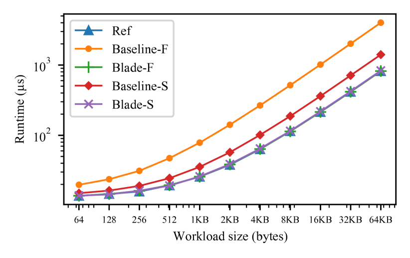
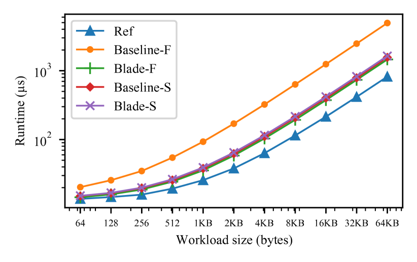
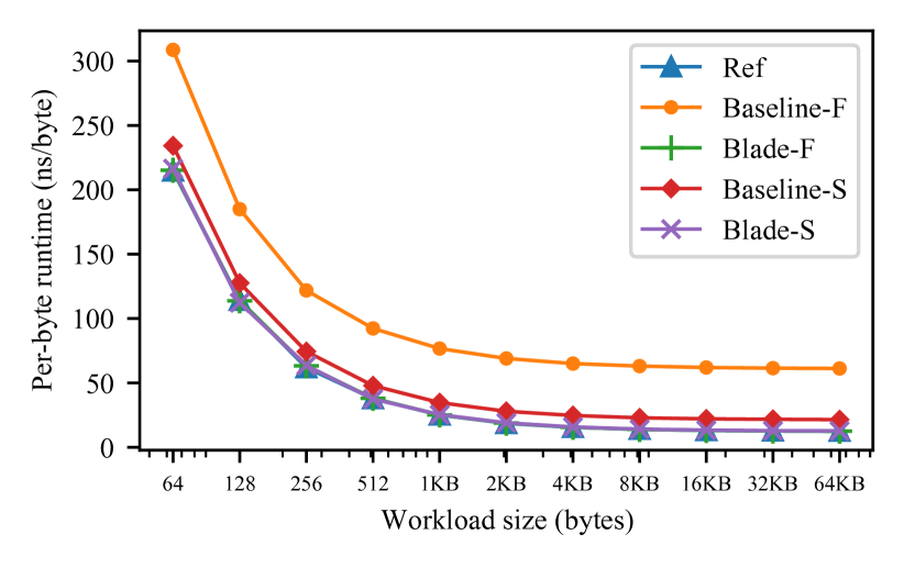
Table 1 showed that the performance overhead for some benchmarks depends heavily on the workload size. We explore this relationship in more detail in Figure 29. Specifically, we see that for low workload sizes, the runtime is dominated by fixed costs for sandbox setup and teardown; the execution of the Wasm code contributes little to the performance. As the workload size increases, the overall performance overhead asymptotically approaches the overhead of the Wasm execution itself. This is shown even more clearly in Figure 30, where we see that the asymptotic overhead for SHA-256 with v1.1 protections is approximately 78% and 99% respectively for Blade-F and Blade-S, while the asymptotic overheads without v1.1 protections are unsurprisingly approximately zero for Blade-F and Blade-S, as they insert no defenses.