Unsupervised Transfer of Semantic Role Models
from Verbal to Nominal Domain

Abstract

Semantic role labeling (SRL) is an NLP task involving the assignment of predicate arguments to types, called semantic roles. Though research on SRL has primarily focused on verbal predicates and many resources available for SRL provide annotations only for verbs, semantic relations are often triggered by other linguistic constructions, e.g., nominalizations. In this work, we investigate a transfer scenario where we assume role-annotated data for the source verbal domain but only unlabeled data for the target nominal domain. Our key assumption, enabling the transfer between the two domains, is that selectional preferences of a role (i.e., preferences or constraints on the admissible arguments) do not strongly depend on whether the relation is triggered by a verb or a noun. For example, the same set of arguments can fill the Acquirer role for the verbal predicate ‘acquire’ and its nominal form ‘acquisition’. We approach the transfer task from the variational autoencoding perspective. The labeler serves as an encoder (predicting role labels given a sentence), whereas selectional preferences are captured in the decoder component (generating arguments for the predicting roles). Nominal roles are not labeled in the training data, and the learning objective instead pushes the labeler to assign roles predictive of the arguments. Sharing the decoder parameters across the domains encourages consistency between labels predicted for both domains and facilitates the transfer. The method substantially outperforms baselines, such as unsupervised and ‘direct transfer’ methods, on the English CoNLL-2009 dataset.

Abstract

This supplementary material includes (1) Reparameterization tricks for estimating the evidence lower bounds; (2) Processing details of the CoNLL data and the NYT data; (3) Configurations of the VAE model and the supervised Factorization baseline model; and (4) Heuristics for identifying arugments of nominal predicates.

1 Introduction

Semantic role labeling (Gildea and Jurafsky, 2002) methods detect the underlying predicate-argument structures of sentences, or, more formally, assign semantic roles to arguments of predicates:

$[\text{Pinocchio}]_{\text{A0}}$ traded the $[\text{book}]_{\text{A1}}$ for a $[\text{ticket}]_{\text{A3}}$.

In this sentence, Pinocchio is labeled as A0, indicating that it is an agent (‘a trader’) of the trading event, whereas book is marked as a patient (A1, ‘an entity being traded’). Semantic-role structures have been shown effective in many NLP tasks, including machine translation (Marcheggiani et al., 2018), question answering (Shen and Lapata, 2007), and summarization (Khan et al., 2015).

Figure 1: Our model transfers argument roles of the verbal predicate (acquired) to the arguments of its nominalization (acquisition). acquired and acquisition share the lemma. Note that we do not rely on any argument alignment.

Most work on SRL relies on supervised learning (He et al., 2017; Marcheggiani and Titov, 2017), and thus requires annotated resources such as PropBank (Palmer et al., 2005) and FrameNet Baker et al. (1998) for English, or SALSA Burchardt et al. (2006) for German. However, the annotated data is available only for a dozen of languages. Moreover, many of these resources cover only verbal predicates, whereas semantic relations are often triggered by other linguistic constructions, such as nominalizations and prepositions. For example, in the popular multilingual CoNLL-2009 dataset Hajič et al. (2009) nominal predicates are provided only for 3 languages (English, Czech, and Japanese). The scarcity of annotated data motivated research into unsupervised SRL methods (e.g., (Swier and Stevenson, 2004; Lang and Lapata, 2011; Titov and Klementiev, 2012; Woodsend and Lapata, 2015)) but these approaches have also focused only on verbal predicates, and, as we will show in our experiments, do not appear effective in the nominal SRL setting. In contrast, nominal predicates, though often neglected in annotation efforts and model development, have been shown crucial in many applications, such as extracting relations from scientific literature Bethard et al. (2008) or events from social media Liu et al. (2012).

In this work, we investigate a transfer scenario, where we assume the presence of role-annotated data for the ‘source’ verbal domain but only unlabeled data for the ‘target’ nominal domain. Our key assumption, driving the transfer between the two domains, is that selectional preferences of a role (i.e., preferences or constraints on the admissible arguments) do not strongly depend on whether the relation is triggered by a verb or a noun. Take the example in Figure 1, semantically similar arguments can fill the A0 (‘entity acquiring something’) role for the verbal predicate acquire and its nominal form acquisition.

We approach the transfer problem from the generative perspective and use the variational autoencoding (VAE) framework Kingma and Welling (2014) or, more specifically, its semi-supervised version Kingma et al. (2014). The semantic role labeler serves as an encoder (predicting roles given a sentence), whereas selectional preferences are captured in the decoder component (generating arguments for the predicting roles). Nominal roles are not labeled in the training data, instead, the autoencoder’s learning objective pushes the labeler to assign roles predictive of the arguments. Sharing the decoder parameters across the domains encourages consistency between labels predicted for both domains. Intuitively, the knowledge is transferred from the verbal domain to the nominal domain.

Similarly, to work on unsupervised semantic role induction in the verbal domain  (Swier and Stevenson, 2004; Lang and Lapata, 2010; Titov and Khoddam, 2015), we focus solely on the argument labeling subtask, and assume that candidate arguments are provided. While we classify gold arguments in our experiments, candidate arguments can also be identified with simple rules (see Section 5.2).

We experiment on the English CoNLL-2009 dataset and compare our approach to baselines. Among the baselines, we consider, (1) a direct transfer approach Zeman and Resnik (2008); Søgaard (2011), which applies a verbal SRL model to the nominal data, and (2) an unsupervised role induction method, which has been shown to achieve state-of-the-art results on the verbal domain Titov and Khoddam (2015). We observe that our model outperforms the strongest baseline models by 6.58% in accuracy and 4.27% in F1, according to supervised and unsupervised evaluation metrics, respectively. Our key contributions can be summarized as follows: (1) we introduce a novel task of transferring SRL models from the verbal to the nominal domain, (2) we propose a simple latent variable model for the task, and (3) we show that the approach compares favourably to existing alternatives.

2 Motivation

Most transferable predicate-role pairs Predicate-Role BC Arguments Overlap Complement (‘non-overlap’) earn AM-TMP 0.845 quarter-num-yearmonthhalf periodearlieragoannualweek pretaxseasontimemonthinterestcurrentnightnowyetbelater neverriseyearstillsummerfridaylatestsecondtax increase A2 0.821 %$-num-centmoremillion share sharpmarkbigsmallratehugelowevenless“dollarminor modestthosetotalunitwagewidearea$ sell A1 0.732 stockshareassetproduct$ bondunitcarstakeit retailthemtruckautoyenartamountcontractmilliongasglass partcddebtexportlincolnrecordfundcarmarket Least transferable predicate-role pairs Predicate-Role BC Complement (‘non-overlap’) interest A2 0.028 interest%seepublicminorinvestorbuyknowithistheircreditorgroupholderu.s.pushbuyer majorourcontrolhalfhejaguarnationp&gthirdwhoseyoumakething rate A1 0.081 interestfilmstocktaxgrowthreturnshowloandefaultdepositdiscountbillprofithimaddeath save$debtprogramacceptassetcdgainworksharethemhebikecancer interest A1 0.087 interestmeshorthigh%buylowstockiyouhethemwehimrateinvestorhigherustheyher oilbuyercongressmanmovementotherteamvoterfanitselfpayment result A2 0.151 resultwillmaygainhavesaycostdeathgrowthremainwouldpricesaleratespend$benefit demandlotproblemitcacancoulddirectdofacefellfundmake direct A2 0.170 directbuyfundmakerbureaubemakestatevetochildhimreview&brotherco.motorunit“ meattorneytvamericaaustraliabudgetfirmforhuttonresearchrighttrust order A1 0.176 orderbuysellheobtainbanhimworthmorecourtbemodelpreventgoodstopherthembank reportallowbackblockbondcarcenterextendfindgaingapget make A1 0.233 autoitsurethemofferloanmovestatementpaymentprinter$effortbehimcaselotmeinvest pointthingyoudepositprogressus%cutsaletripusecomment

Table 1: Predicate-role pairs with the most and least similar selectional preferences, as measured with the Bhattacharyya coefficient (BC), the larger the more similar. The intensity of green is used to indicate the degree of positive contribution of an argument to BC. The intensity of blue and red indicates the negative contribution: the blue arguments appear predominantly with verbal predicates, where the red (= italic) words are mostly arguments of nominalizations.

As discussed above, our approach hinges on the assumption that selectional preferences of a role (e.g., A0) are similar for verbal predicates (e.g., acquire) and their nominalizations (e.g., acquisition). In this section, we verify this assumption through analyzing the verbal PropBank (Palmer et al., 2005) and nominal NomBank (Meyers et al., 2004) resources, or, more formally, their CoNLL-2009 version (Hajič et al., 2009).

As in the rest of the paper, we rely on lemmas and a nominalization list to relate verbal predicates (e.g., earn) to their nominal forms (e.g., earning and earner). In what follows, we use lemmas to refer to predicates. To ensure the reliability of our metrics, we consider predicate-role pairs which appear at least 100 times, resulting in 65 predicate-role pairs, and take only frequent arguments (a cut-off of 20).

First, we would like to identify the predicate-role pairs which have the most and the least similar selectional preferences across the domains. To do this, for every predicate-role pair, we collect its arguments in the verbal domain and arguments in the nominal domain, lemmatize them and measure the distance between the two argument samples. We rely on the Bhattacharyya coefficient (BC), a standard way of measuring the amount of overlap between statistical samples. As we can see from Table 1, BC for (earn, AM-TMP) and (increase, A2) are the highest ($0.845$ and $0.821$), indicating that the selectional preferences for the nominal and verbal domains are very similar. In contrast, the similarity is very low ($0.028$ and $0.081$) for (interest, A2) and (rate, A1). Arguments for these role-predicate pairs almost do not overlap between their verbal and nominal forms.

Second, in order to understand the reason for this discrepancy, we measure the contribution of individual arguments. We define the contribution as the change to BC, caused by removing all occurrences of the argument from the samples. For example, removing quarter for the predicate-role pair (earn, AM-TMP) causes the largest drop in BC, while taking out pretax results in the largest jump. We can see that some of the largest discrepancies are due to peculiarities of the NomBank annotation guidelines. The most obvious one is the presence of self-loops, i.e., nominal predicates in NomBank can take themselves as arguments. For example, A2 for the predicate direct is defined as ‘movement direction’, and the nominalized predicate direction is always labeled as A2. Other problematic cases are due to multi-word expressions, such as auto makers or pretax earnings that do not have frequent verbal counterparts.

Still, even if we ignore annotation divergences, we see that our assumption is only an approximation. Nevertheless, it is accurate for a subset of predicate-role pairs. We hypothesize that, due to parameter sharing in our model, easier ‘transferable’ cases will help us to learn to label in harder ‘non-transferable’ ones.

3 Transfer Learning

In our setting, we are provided with a labeled dataset $\mathcal{X}_{v}$ for the source verbal domain but the role labels are not annotated in the target nominal data $\mathcal{X}_{n}$. Our goal is to produce an SRL model for the target. Given a predicate $p$ in a sentence $\mathbf{w}$, a semantic role labeler needs to assign roles $\mathbf{y}=y_{1},\ldots,y_{m}$ to arguments $\mathbf{a}=a_{1},\ldots,a_{m}$. We consider dependency-based SRL (see Figure 1), i.e., we label syntactic heads of argument phrases (e.g., ‘positions’ instead of the entire span ‘equity positions’).

In order to exploit unlabeled data we will use the generative framework, or, more specifically, semi-supervised VAEs (Kingma et al., 2014). We will start by describing the generative model, and then show how it can be integrated in the semi-supervised VAE objective and used to produce a discriminative semantic role labeler.

3.1 Generative model

The generative model defines the process of producing arguments $\mathbf{a}$ relying on roles $\mathbf{y}$ and a continuous latent variable $\mathbf{z}$. The variable $\mathbf{z}$ can be regarded as a latent code encoding properties of the proposition (i.e., the triple $p$, $\mathbf{y}$ and $\mathbf{a}$). We start by drawing the roles and the code from priors:

$$p(\mathbf{y})=\prod_{i}p(y_{i});\quad p(\mathbf{z})=\mathcal{N}(\mathbf{z}|\mathbf{0},\mathbf{I}),$$

where, for simplicity, we assume that $p(y_{i})$ is the uniform distribution. We then generate arguments (formally, argument lemmas) using an autoregressive selectional preference model:

$$p_{\theta}(\mathbf{a}|\mathbf{y},\mathbf{z})=\prod_{i}{p_{\theta}(a_{i}|\mathbf{y},\mathbf{a}_{<i},\mathbf{z},p)},$$ (1)

where $\mathbf{a}_{<i}=(a_{1},\ldots,a_{i-1})$. This contrasts with most previous work in selectional preference modeling, which assumes that arguments are conditionally-independent (e.g., Ritter et al. (2010)). As we will see in our ablations, both using the latent code and conditioning on other arguments is beneficial. On nominal data $\mathbf{y}$ is latent and the marginal likelihood is given by

$$T_{\theta}(\mathbf{a})\!=\!\log\!\int\sum_{\mathbf{y}}p(\mathbf{y})p(\mathbf{z})p_{\theta}(\mathbf{a}|\mathbf{y},\mathbf{z})\,d\mathbf{z}\,.$$ (2)

Recall that we reuse the generative model across nominal and verbal domains. As the preferred argument order is different for verbal and nominal predicates, our model needs to be permutation-invariant or, equivalently, model bags of labeled arguments rather than their sequences Vinyals et al. (2015). We achieve this by replacing the maximum likelihood objective $T_{\theta}(\mathbf{a})$ with pseudolikelihood Besag (1977). In other words, we replace $p_{\theta}(\mathbf{a}|\mathbf{y},\mathbf{z})$ in Equation 2 with the following term:

$$f_{\theta}(\mathbf{a},\mathbf{y},\mathbf{z})=\prod_{i}{p_{\theta}(a_{i}|\mathbf{y},\mathbf{a}_{-i},\mathbf{z},p)},$$ (3)

where $\mathbf{a}_{-i}$ refers to all arguments in $\bf{a}$ but the $i$-th, resulting in the objective

$$\hat{T}_{\theta}(\mathbf{a})\!=\!\log\!\int\sum_{\mathbf{y}}p(\mathbf{y})p(\mathbf{z})f_{\theta}(\mathbf{a},\mathbf{y},\mathbf{z})\,d\mathbf{z}\,.$$ (4)

Intuitively, when predicting an argument, the model can access all other arguments. Furthermore, to fully get rid of the order information, we ensure that $p_{\theta}(a_{i}|\mathbf{y},\mathbf{a}_{-i},\mathbf{z},p)$ is invariant to joint reordering of the arguments $\mathbf{a}_{-i}$ and their roles $\mathbf{y}_{-i}$. The neural network achieving this property is described in Section 4.1.

3.2 Argument reconstruction

Optimizing the pseudolikelihood involves intractable marginalization over the latent variables $\mathbf{z}$ and $\mathbf{y}$. With VAEs, we instead maximize its lower bound:

$$\hat{T}_{\theta}(\mathbf{a}) \geq\mathbb{E}_{q_{\phi}(\mathbf{y},\mathbf{z}|\mathbf{w})}\left[\log f_{\theta}(\mathbf{a},\mathbf{y},\mathbf{z})\right]$$ (5)

$$-\text{KL}(q_{\phi}(\mathbf{y},\mathbf{z}|\mathbf{w})||p(\mathbf{y})p(\mathbf{z}))=\mathcal{U}_{\theta,\phi}(\mathbf{w})\,,$$

where $q_{\phi}(\mathbf{y},\mathbf{z}|\mathbf{w})$ is an estimate of the intractable true posterior, provided by an inference network, a neural network parameterized by $\phi$. The first term in Equation 5 is the autoencoder’s reconstruction loss: the inference network serves as an encoder and the selectional preference model as the decoder. The other term can be regarded as a regularizer on the latent space. We also factorize the inference network into two components: a semantic role labeler $q_{\phi}(\mathbf{y}|\mathbf{w})$ and a latent code generator $q_{\phi}(\mathbf{z}|\mathbf{w})$.

Figure 2: An example of predicting the argument recent with the VAE model. The underlined words in $\mathbf{w}$ are argument fillers. We replace them with a special symbol ’_’ and obtain $\mathbf{w}_{-\mathbf{a}}$. $\mathbf{x}_{1}$ is the input to the decoder model. It is represented as the concatenation of the predicate (acquire) embedding, the latent code $\mathbf{z}$, the embedding of the recent’s role (ADV), and contexts from the other roles and arguments. Note that role labels are sampled from $q_{\phi}(\mathbf{y}|\cdot)$; we are using lemmas for the nominal predicate acquisition and the arguments.

On the verbal data $\mathbf{y}$ is observed, and the pseudo-likelhood lower bound becomes:

$$\mathcal{L}_{\theta,\phi}(\mathbf{w},\mathbf{y}) =\mathbb{E}_{q_{\phi}(\mathbf{z}|\mathbf{w})}\left[\log f_{\theta}(\mathbf{a},\mathbf{y},\mathbf{z})\right]$$ (6)

$$-\text{KL}(q_{\phi}(\mathbf{z}|\mathbf{w})||p(\mathbf{z}))\,.$$

We will describe the architecture of both inference networks in Section 4.

3.3 Joint objective

While using the objectives $\mathcal{U}_{\theta,\phi}(\mathbf{w})$ and $\mathcal{L}_{\theta,\phi}(\mathbf{w},\mathbf{y})$ can already faciliate the transfer, as standard with semi-supervised VAEs, we use an extra discriminative term which encourages the semantic role labeler to predict correct labels on the labeled verbal data:

$$\mathcal{D}_{\phi}(\mathbf{w}_{v},\mathbf{y}_{v})=\log q_{\phi}(\mathbf{y}_{v}|\mathbf{w}_{v})\,.$$ (7)

In practice, we share the semantic role labeler $q_{\phi}(\mathbf{y}|\mathbf{w})$ across nominal and verbal domains. Note that though the parameters $\phi$ are shared, the labeler relies on the predicate and the sentence and can easily detect which domain it is applied to. In other words, sharing the labeler’s parameters provides only a soft inductive bias rather than a hard constraint. The parameter sharing is the reason for why $q_{\phi}(\mathbf{y}_{v}|\mathbf{w}_{v})$ can benefit from accessing the entire sentence $\bf{w}$, rather than using only the arguments $\bf{a}$, as would have followed from the posterior estimation perspective.

To summarize, the overall loss function is minimized with respect to $\theta$ and $\phi$:

$$\mathcal{J_{\theta,\phi}} =-\sum_{\mathbf{w}_{n}\sim\mathcal{X}_{n}}\mathcal{U}_{\theta,\phi}(\mathbf{w}_{n})$$ (8)

$$-\sum_{(\mathbf{w}_{v},\mathbf{y}_{v})\sim\mathcal{X}_{v}}\mathcal{L}_{\theta,\phi}(\mathbf{w}_{v},\mathbf{y}_{v})+\alpha\cdot\mathcal{D}_{\phi}(\mathbf{w}_{v},\mathbf{y}_{v})\,,$$

where $\alpha$ is a hyper-parameter balancing the relative importance of the discriminative term. Note that the estimation of the lower bounds requires sampling from $q_{\phi}(\mathbf{y}|\mathbf{w})$ and $q_{\phi}(\mathbf{z}|\mathbf{w})$, which is not differentiable. This, together with the presence of discrete latent variables, makes the optimization challenging. As a remedy, for $\mathbf{z}$ we employ the reparametrization trick (Kingma et al., 2014); for $\mathbf{y}$ we resort to the Gumbel-Softmax relaxation (Jang et al., 2017; Maddison et al., 2017). Details can be found in Appendix A.

4 Component Architecture

In this section, we formally describe every component of our VAE. A schematic overview of the model is illustrated in Figure 2.

4.1 Decoder $f_{\theta}(\mathbf{a},\mathbf{y},\mathbf{z})$

As shown on the right in Figure 2, the neural network computing $p_{\theta}(a_{i}|\mathbf{y},\mathbf{a}_{-i},\mathbf{z},p)$ takes as input the concatenation of the predicate embedding $p$, the latent code $\mathbf{z}$, the role embedding $y_{i}$ as well as the representations of the other arguments $\mathbf{c}_{\mathbf{a}_{-i}}$ and the other roles $\mathbf{c}_{\mathbf{y}_{-i}}$:

$$\mathbf{c}_{\mathbf{a}_{-i}} =\frac{1}{m-1}\sum_{j\neq i}\mathbf{v}_{a_{j}}\,,$$

$$\mathbf{c}_{\mathbf{y}_{-i}} =\frac{1}{m-1}\sum_{j\neq i}\mathbf{v}_{y_{j}}\,,$$

where $\mathbf{v}_{a_{j}}$ and $\mathbf{v}_{y_{j}}$ are argument embedding and role embedding, respectively. The resulting vector is passed through a two-layer feedforward network, with the tanh non-linearities, followed with the softmax over argument lemmas. The arguments $\mathbf{a}_{-i}$ and their roles $\mathbf{y}_{-i}$ are encoded via the mean operation over their embeddings, ensuring that the resulting model is invariant to their order.

4.2 Encoder models

4.2.1 Semantic role labeler $q_{\phi}(\mathbf{y}|\mathbf{w})$

We adapt the SRL model of He et al. (2017) to dependency-based SRL. Specifically, a highway BiLSTM model first encodes arguments into contextualized representations. Then roles are predicted independently using the softmax function. Note that the SRL model is the only component retained after training with the objective  (defined in Equation 8) and used at test time. Other model components can be discarded.

4.2.2 Latent code predictor $q_{\phi}(\mathbf{z}|\mathbf{w})$

Formally, as the inference network estimates the posterior $p(\mathbf{z}|\mathbf{a})$, it needs to rely on all arguments $\mathbf{a}$ and cannot benefit from any other information in $\mathbf{w}$. In practice, using such an inference network would result in posterior collapse: the model would ignore discrete variables $\mathbf{y}$ and rely on $\mathbf{z}$ to pass information to the decoder. In order to prevent this, the network relies on $\mathbf{w}_{-\mathbf{a}}$, i.e., the sentence with all the predicate’s arguments masked. In other words, it can derive relevant features only from the context. In our implementation, we input $\mathbf{w}_{-\mathbf{a}}$ to a BiLSTM model, then a mean-pooling layer is applied to the BiLSTM hidden states. Finally, the mean vector $\mathbf{\mu}_{\phi}(\mathbf{w}_{-\mathbf{a}})$ and the log-covariances $\log\mathbf{\sigma}_{\phi}(\mathbf{w}_{-\mathbf{a}})$ are output by an affine layer.

5 Experiments

The main results are presented in Section 5.3. As unsupervised baselines cannot be evaluated using standard metrics, we compare with them using clustering metrics in Section 5.4.

5.1 Datasets and model configurations

Dataset: We use the English CoNLL-2009 (CoNLL) dataset (Hajič et al., 2009) with standard data splits. We separate it into the verbal and nominal domains by predicate types: verb vs noun. For a prepositional argument such as at in the prepositional phrase ‘at the library’, we instead use as the argument the headword (library in this case) of the noun phrase following the preposition. Moreover, we keep 15 frequent roles shared by the two domains (a cut-off of 3). Data statistics and processing details can be found in Appendix B.1.

Data augmentation: Transfer learning models benefit from labeled data in the source domain. To obtain extra labeled verbal data, we pre-train a verbal semantic role labeler and apply it to the verbal predicates in the New York Times Corpus (NYT) (Sandhaus, 2008) (details in Appendix B.2). For each predicate in the unlabeled nominal training data, we select 1000 random instances with that predicate from the automatically-labeled NYT data and add them to our verbal training data.

Model configurations: Our model is implemented using AllenNLP (Gardner et al., 2018) and relies on ELMo (Peters et al., 2018). The dimension of the latent code $\mathbf{z}$ is set to 100. The embeddings of predicates and roles are randomly initialized. We pre-train lemma embeddings for arguments on the Wikipedia data (Müller and Schuetze, 2015), which is lemmatized by the lemmatizer Lemming (Müller et al., 2015). All the embeddings are of dimension 100 and are tunable during training. We optimize the model using the Adadelta (Zeiler, 2012), with the learning rate set to 1. Appendix C provides extra details.

5.2 Automatic argument identification

We start by demonstrating that unlabeled arguments can be extracted with relatively simple rules. Inspired by heuristics from Lang and Lapata (2011) developed for verbal predicates, we define 5 simple rules; these rules use syntactic dependency structures and yield 77% F1 in identification. Appendix D elaborates on the rules. The distribution of labels of the extracted arguments is however different from the one in gold standard. E.g., A0 is almost twice more frequent among gold arguments than extracted ones. Thus, to make our findings independent of the (imperfect and simple) rules, in main experiments we focus on classifying arguments taken from ground truth.

5.3 Supervised evaluation

5.3.1 Baseline models

We consider the following three baseline models:

• Most-frequent assigns an argument to its most frequent role given the predicate in the verbal training data. When the predicate and the argument do not co-occur, it assigns the argument to the most frequent role of the predicate.

• Factorization estimates the compatibility of a role $y_{i}$ with predicate $p$ and argument $a_{i}$ using the bilinear score $s(a_{i},y_{i},p)=\mathbf{v}_{a_{i}}^{T}\mathbf{W}_{y_{i}}\mathbf{v}_{p}+\mathbf{v}_{a_{i}}^{T}\mathbf{w}_{y_{i}}$, where $\mathbf{v}_{a_{i}}$ and $\mathbf{v}_{p}$ are argument and predicate embeddings, respectively; $\mathbf{W}_{y_{i}}$ and $\mathbf{w}_{y_{i}}$ are a matrix embedding and a vector embedding of the role, respectively. The scoring function is similar to the one used in  Titov and Khoddam (2015) but we estimate it on the labeled verbal data. See Appendix C.1 for details.

• Direct-transfer is our semantic role labeler estimated only on the verbal data (i.e., using the loss $\mathcal{D}_{\phi}$ in Equation  7) and applied to the nominal data.

Model A0 A1 A2 AM-* All Most-frequent 62.45 67.13 17.69 42.11 56.51 Factorization 53.76 56.45 3.65 27.03 44.48 Direct-transfer 67.52 64.72 24.13 40.78 55.85 Ours 71.43 70.09 19.78 62.04 63.09 -Self-loop 66.44 73.80 27.26 63.07 64.51

Table 2: F1 scores on the CoNLL nominal test data.

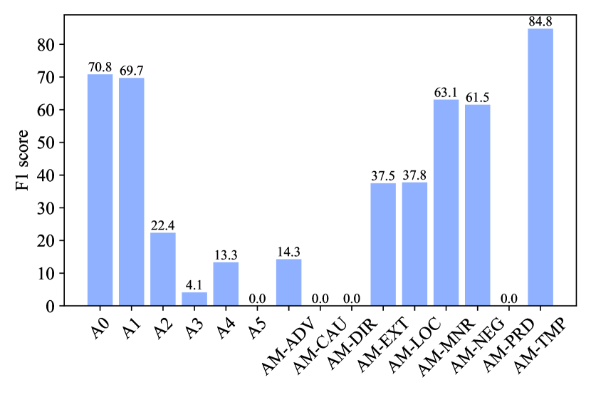
Figure 3: F1 score of our model, per role, on the nominal devel data.

5.3.2 Experimental results

Our model achieves the best overall scores (Table 2). Most-frequent and Factorization directly estimate selectional preferences on the verbal domain and apply them to the nominal one, while in our approach we share a selectional preference model to bootstrap our labeler. The lower scores of these baselines suggest that it is indeed crucial to distill this weak signal into the SRL model rather than relying on it at test time. The improvement over Direct-transfer shows that we genuinely benefit from using unlabeled nominal data.

The performance varies greatly across the roles, with the best results for proto-agent (A0) and proto-patient (A1) roles and much weaker for A2-A5 and adjunt / modifier roles (AM-*). Roles A2-A5 are hard even for supervised systems, as they are predicate-specific (i.e., A4 for one predicate may have nothing to do with A4 for another). The low scores for AM-* are more surprising, as their selectional preferences should not depend much on the predicate. Looking into individual roles in Figure 3, we see that our model is accurate for AM-TMP, but not for AM-ADV and AM-MNR. While for AM-TMP lemmas of arguments are very similar across verbal and nominal domains (see also top line in Table 1), this is not the case for AM-ADV and AM-MNR. E.g., while frequent AM-ADV arguments in the verbal domain are so and while, these lemmas do not appear as AM-ADV arguments in the nominal data.

The nominal data contains self-loops, i.e., cases where a predicate is an argument of itself (see Section 2). This annotation decision is controversial and most other formalism Banarescu et al. (2013) does not use them. Their presence negatively affects our approach as the verbal data has no self-loops. As expected, our model scores better when these arguments are removed at test time (-Self-loop in Table 2).

Model full -$\mathbf{z}$ -joint -augment Accuracy $\mathbf{62.86}_{\pm 0.57}$ $60.72_{\pm 1.27}$ $51.60_{\pm 2.12}$ $57.20_{\pm 0.86}$

Table 3: Accuracy on the CoNLL nominal devel data.

5.3.3 Ablation study

We investigate the importance of the latent code $\mathbf{z}$, joint modeling of arguments (joint), and data augmentation (augment). We consider the VAE model with all the three components as the full model. Then we ablate the model by removing each of the three components individually. We train each model five times with different random seeds and report the mean and unbiased standard deviation of model accuracies. Table 3 summarizes the results. We can see that all the three components are indispensable. The smaller standard deviation of the full model also suggests that they help stabilize the training process.

We also study the impact of augmented-data size on the model performance. Figure 4 illustrates that the model accuracy consistently grows when increasing the number of labeled verbal examples (per predicate type). We leave using more data for augmentation for future work.

Models PU CO F1 AllA0 45.76 100.0 62.79 SyntFun 63.42 66.81 65.07 Arg2vec 64.31 64.36 64.33 Factorization 75.29 52.77 62.05 Most-frequent 66.48 75.10 70.53 Direct-transfer 66.43 69.33 67.85 Ours 71.38 78.56 74.80

Table 4: Clustering results on the CoNLL nominal training data.

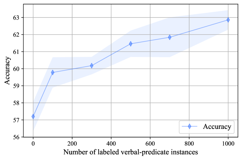
Figure 4: Accuracy on the CoNLL nominal devel data.

5.4 Unsupervised evaluation

5.4.1 Baseline models and evaluation metrics

We consider the following baseline models:

• AllA0 assigns all arguments to A0, the most frequent role in the data.

• SyntFun is a standard baseline in verbal semantic role induction. Each cluster corresponds to a syntactic function (i.e., a dependency relation of an argument to its syntactic head).

• Arg2vec exploits the similarities among arguments in the embeddings space. It uses the agglomerative algorithm to cluster the pre-trained lemma embeddings of arguments. To be comparable with our model, we set the cluster number to 15, the number of roles in the verbal data.

• Factorization is the verbal semantic role induction method of  Titov and Khoddam (2015), which achieves state-of-the-art performance on the verbal domain. We use their code.

• Most-frequent and Direct-transfer are the supervised models from Section 5.3.1 but evaluated using unsupervised metrics.

Evaluation metrics: As standard in role induction literature, we evaluate models using clustering metrics: purity (PU), collocation (CO), and their harmonic mean F1 Lang and Lapata (2010).

5.4.2 Experimental results

Table 4 presents clustering results of different models. We can see that SyntFun surpasses AllA0 by 2.28 in F1 measure, suggesting that syntactic functions remain good predictors of semantic roles in the nominal domain. However, Factorization does not work well when applied to the nominal data. Our model performs best, ourperforming the strongest baseline, Most-frequent, by 4.27% F1.

6 Additional related work

Transfer learning, while popular for SRL, has focused on cross-lingual transfer. Work in this direction uses annotation projection (Padó and Lapata, 2009; van der Plas et al., 2011; Aminian et al., 2019) or relies on shared feature representation (Kozhevnikov and Titov, 2013). We are the first, as far as we know, to consider transfer across linguistic constructions.

Semi-supervised Learning with VAEs is proposed by Kingma et al. (2014) for classification problem. The VAEs have been adapted for various tasks in semi-supervised setting. Most of them consist of both continuous and discrete latent variables (Xu et al., 2017; Zhou and Neubig, 2017; Chen et al., 2018). Our model follows this line of work. However, we focus on a transfer learning task since the labeled and unlabeled data come from different domains.

7 Conclusion

We defined a new task of transferring semantic role models from the labeled verbal domain to the unlabeled nominal domain. We proposed to exploit the similarity in selectional preferences across the domains and introduced a VAE model realizing this intuition. Our model outperformed both supervised and unsupervised baselines.

In the future, we would like to explore alternative approaches to transfer learning (e.g., using paraphrase models or pivoting via parallel data), and consider other languages and other linguistic constructions (e.g., prepositions Srikumar and Roth (2013)). It would also be interesting to use SemLink Palmer (2009) or AMR Banarescu et al. (2013) to evaluate transfer quality.

Supplementary Material

Appendix A Reparameterization trick

We use gradient-based optimization to maximize the evidence lower bounds. It involves sampling from $q_{\phi}(\mathbf{y}|\mathbf{w})$ and $q_{\phi}(\mathbf{z}|\mathbf{w})$, which is not differentiable, This, together with the presence of discrete latent variables makes the optimization challenging. As a remedy, for $\mathbf{z}$ we employ the reparametrization trick (Kingma et al., 2014) and define $\mathbf{z}$ as a deterministic variable:

$$\mathbf{z}=\mathbf{\mu}_{\phi}(\mathbf{w})+\sqrt{\mathbf{\sigma}_{\phi}(\mathbf{w})}*\mathbf{\epsilon},\quad\mathbf{\epsilon}\sim\mathcal{N}(\mathbf{0},\mathbf{I})\,.$$

This sampling process is equivalent to sampling $\mathbf{z}$ from $\mathcal{N}(\mathbf{z}|\mathbf{\mu}_{\phi}(\mathbf{w}),\text{diag}(\mathbf{\sigma}_{\phi}(\mathbf{w})))$ directly. However, it removes the non-differentiable sampling process from gradient back-propagation path. For $\mathbf{y}$ we resort to the Gumbel-Softmax relaxation (Jang et al., 2017; Maddison et al., 2017), which relies on the Gumbel-Max Maddison et al. (2014) to draw samples $y$ from a categorical distribution over the role label space:

$$y=\operatorname*{argmax}_{i}[g_{i}+\log\pi_{i}],\quad g_{i}\sim\text{Gumbel}(0,1)\,,$$

where for $i\in\{1,\ldots,n_{r}\}$, $\pi_{i}$ specifies the probability $i$-th role label and $\sum_{i}\pi_{i}=1$; $g_{i}$ is drawn independently from the Gumbel distribution. To avert the non-differentiable $\operatorname*{argmax}$, we represent $y$ as one-hot vector and approximate it using the softmax function: $y_{i}=\frac{1}{Z}\exp(g_{i}+\log\pi_{i})$ where $Z=\sum_{i}\exp(g_{i}+\log\pi_{i})$.

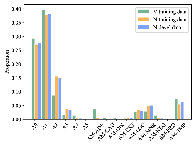
Figure 5: Proportion of each role in the verbal (V) training data and the nominal (N) data.

Appendix B Data

B.1 CoNLL data processing

We apply verbalization to nominal predicates of the English CoNLL-2009 (CoNLL) dataset (Hajič et al., 2009), mapping nouns to their verb forms according to the morph-verbalization list . Then we select a set of shared verb predicates between the two domains and retain only instances having these shared predicates. Moreover, we keep only the following 15 frequent role labels in the two domains (a cut-off of 3): A0, A1, A2, A3, A4, A5, AM-ADV, AM-CAU, AM-DIR, AM-EXT, AM-LOC, AM-MNR, AM-NEG, AM-PRD, AM-TMP. Statistics of the resulting datasets are shown in Table 5. Figure 5 shows proportions of the 15 roles in the final data. In training, we use only the predicates attested with at least 20 instances in the nominal domain and at least 10 instances in the verbal domains, This rules out infrequent predicates which either trivially lead to a high score or lack labeled data to learn from.

train dev test # pred- # sample # pred- # sample # pred- # sample V 1025 68461 387 1404 454 2223 N 1025 38283 533 2456 582 3955

Table 5: Number of instances (# sample) and predicate forms (# pred-) in the verbal (V) and nominal (N) domains of the processed CoNLL data.

B.2 Verbal data augmentation

We pre-train a semantic role labeler on the CoNLL verbal training data. The model gives rise to an F1 score of 89.2 on the CoNLL verbal development data, which is strong enough. Then we apply it to the verbal predicates in the New York Times Annotated Corpus (NYT) (Sandhaus, 2008) and obtain extra labeled verbal data.

The preprocessing of the NYT data is as follows: first we tokenize and segment the NYT data into sentences and rule out sentences having more than 45 words. Then we lemmatize each sentence and label it with part-of-speech (POS) tags using a pre-trained lemmatizer (Müller et al., 2015). After that, we employ the following heuristic to identify predicates in the sentences: we collect all pairs of predicate and its POS tag from the CoNLL training data, then we search for matches to these pairs of predicate and POS tag in the NYT data. For every complete match with the same predicate and POS tag, we count it as a predicate occurrence. Finally, we extract verbal-predicate data and retain instances which share the same set of verbal predicates as in the processed CoNLL data.

Appendix C Model parameters

The semantic role model $q_{\phi}(\mathbf{y}|\cdot)$ uses the same highway BiLSTM encoder as in He et al. (2017). The encoder model $q_{\phi}(\mathbf{z}|\cdot)$ also uses a highway BiLSTM but with only one layer (interested readers are referred to He et al. (2017)).

C.1 Supervised baseline model

Factorization estimates the compatibility of a role $y_{i}$ with predicate $p$ and argument $a_{i}$:

$$s(a_{i},y_{i},p)=\mathbf{v}_{a_{i}}^{T}\mathbf{W}_{y_{i}}\mathbf{v}_{p}+\mathbf{v}_{a_{i}}^{T}\mathbf{w}_{y_{i}}\,,$$

where $\mathbf{v}_{a_{i}}$ and $\mathbf{v}_{p}$ are argument and predicate embeddings, respectively; $\mathbf{W}_{y_{i}}$ and $\mathbf{w}_{y_{i}}$ is a matrix embedding and a vector embedding of the role, respectively. The model is trained to maximize the conditional log-likelihood of $a_{i}$ given $p$ and $y_{i}$:

$$\log p(a_{i}|p,y_{i})=\log\frac{\exp(s(a_{i},y_{i},p))}{\sum_{j}\exp(s(a_{j},y_{i},p))}\,.$$

We use the pre-trained lemma embeddings for arguments and randomly initialize predicate embeddings. Both the embeddings are of dimension 100 and are tunable during training.

Appendix D Argument identification

We use the following five rules to heuristically identify arguments for nominal predicates. The heuristics rely only on gold syntactic dependency structures and part-of-speech tags. Initially, all words in a sentence are treated as non-arguments.

• Determinators and punctuations are removed from consideration

• Any of a predicate’s dependents that appears before the predicate are labeled as arguments (i.e., the dependent’s word index is smaller than the predicate’s word index). When it appears after the predicate, it is labeled as an argument if and only if it is a preposition.

• All preposition siblings of a predicate are labeled as arguments if and only if the predicate does have any dependents.

• All SBJ siblings of a predicate are labeled as arguments if and only if the predicate’s relation to its head is OBJ.

• The closest word to a predicate that appears before the predicate and has the dependency label SBJ is labeled as an argument if and only if the predicate does not have any dependents preceding the predicate.

References

- Aminian et al. (2019) Maryam Aminian, Mohammad Sadegh Rasooli, and Mona Diab. 2019. Cross-lingual transfer of semantic roles: From raw text to semantic roles. In Proceedings of the 13th International Conference on Computational Semantics - Long Papers, pages 200–210, Gothenburg, Sweden. Association for Computational Linguistics.
- Baker et al. (1998) Collin F. Baker, Charles J. Fillmore, and John B. Lowe. 1998. The Berkeley FrameNet project. In COLING 1998 Volume 1: The 17th International Conference on Computational Linguistics.
- Banarescu et al. (2013) Laura Banarescu, Claire Bonial, Shu Cai, Madalina Georgescu, Kira Griffitt, Ulf Hermjakob, Kevin Knight, Philipp Koehn, Martha Palmer, and Nathan Schneider. 2013. Abstract meaning representation for sembanking. In Proceedings of the 7th Linguistic Annotation Workshop and Interoperability with Discourse, pages 178–186, Sofia, Bulgaria. Association for Computational Linguistics.
- Besag (1977) Julian Besag. 1977. Efficiency of pseudolikelihood estimation for simple gaussian fields. Biometrika, 64(3):616–618.
- Bethard et al. (2008) Steven Bethard, Zhiyong Lu, James H. Martin, and Lawrence Hunter. 2008. Semantic role labeling for protein transport predicates. BMC Bioinformatics, 9(1):277.
- Burchardt et al. (2006) Aljoscha Burchardt, Katrin Erk, Anette Frank, Andrea Kowalski, Sebastian Padó, and Manfred Pinkal. 2006. The SALSA corpus: a German corpus resource for lexical semantics. In Proceedings of the Fifth International Conference on Language Resources and Evaluation (LREC’06), Genoa, Italy. European Language Resources Association (ELRA).
- Chen et al. (2018) Mingda Chen, Qingming Tang, Karen Livescu, and Kevin Gimpel. 2018. Variational sequential labelers for semi-supervised learning. In Proceedings of the 2018 Conference on Empirical Methods in Natural Language Processing, pages 215–226, Brussels, Belgium. Association for Computational Linguistics.
- Gardner et al. (2018) Matt Gardner, Joel Grus, Mark Neumann, Oyvind Tafjord, Pradeep Dasigi, Nelson F. Liu, Matthew Peters, Michael Schmitz, and Luke Zettlemoyer. 2018. AllenNLP: A deep semantic natural language processing platform. In Proceedings of Workshop for NLP Open Source Software (NLP-OSS), pages 1–6, Melbourne, Australia. Association for Computational Linguistics.
- Gildea and Jurafsky (2002) Daniel Gildea and Daniel Jurafsky. 2002. Automatic labeling of semantic roles. Computational Linguistics, 28(3):245–288.
- Hajič et al. (2009) Jan Hajič, Massimiliano Ciaramita, Richard Johansson, Daisuke Kawahara, Maria Antònia Martí, Lluís Màrquez, Adam Meyers, Joakim Nivre, Sebastian Padó, Jan Štěpánek, Pavel Straňák, Mihai Surdeanu, Nianwen Xue, and Yi Zhang. 2009. The CoNLL-2009 shared task: Syntactic and semantic dependencies in multiple languages. In Proceedings of the Thirteenth Conference on Computational Natural Language Learning (CoNLL 2009): Shared Task, pages 1–18, Boulder, Colorado. Association for Computational Linguistics.
- He et al. (2017) Luheng He, Kenton Lee, Mike Lewis, and Luke Zettlemoyer. 2017. Deep semantic role labeling: What works and what’s next. In Proceedings of the 55th Annual Meeting of the Association for Computational Linguistics (Volume 1: Long Papers), pages 473–483, Vancouver, Canada. Association for Computational Linguistics.
- Jang et al. (2017) Eric Jang, Shixiang Gu, and Ben Poole. 2017. Categorical reparameterization with gumbel-softmax. In Proceedings of the 5th International Conference on Learning Representations.
- Khan et al. (2015) Atif Khan, Naomie Salim, and Yogan Jaya Kumar. 2015. A framework for multi-document abstractive summarization based on semantic role labelling. Applied Soft Computing, 30:737 – 747.
- Kingma and Welling (2014) Diederik P Kingma and Max Welling. 2014. Auto-encoding variational bayes. In Proceedings of the 2nd International Conference on Learning Representations.
- Kingma et al. (2014) Durk P Kingma, Shakir Mohamed, Danilo Jimenez Rezende, and Max Welling. 2014. Semi-supervised learning with deep generative models. In Z. Ghahramani, M. Welling, C. Cortes, N. D. Lawrence, and K. Q. Weinberger, editors, Advances in Neural Information Processing Systems 27, pages 3581–3589. Curran Associates, Inc.
- Kozhevnikov and Titov (2013) Mikhail Kozhevnikov and Ivan Titov. 2013. Cross-lingual transfer of semantic role labeling models. In Proceedings of the 51st Annual Meeting of the Association for Computational Linguistics (Volume 1: Long Papers), pages 1190–1200, Sofia, Bulgaria. Association for Computational Linguistics.
- Lang and Lapata (2010) Joel Lang and Mirella Lapata. 2010. Unsupervised induction of semantic roles. In Human Language Technologies: The 2010 Annual Conference of the North American Chapter of the Association for Computational Linguistics, pages 939–947, Los Angeles, California. Association for Computational Linguistics.
- Lang and Lapata (2011) Joel Lang and Mirella Lapata. 2011. Unsupervised semantic role induction via split-merge clustering. In Proceedings of the 49th Annual Meeting of the Association for Computational Linguistics: Human Language Technologies, pages 1117–1126, Portland, Oregon, USA. Association for Computational Linguistics.
- Liu et al. (2012) Xiaohua Liu, Zhongyang Fu, Xiangyang Zhou, Furu Wei, and Ming Zhou. 2012. Collective nominal semantic role labeling for tweets. In Proceedings of the Twenty-Sixth AAAI Conference on Artificial Intelligence, pages 1685–1691. AAAI Press.
- Maddison et al. (2017) Chris J Maddison, Andriy Mnih, and Yee Whye Teh. 2017. The concrete distribution: A continuous relaxation of discrete random variables. In Proceedings of the 5th International Conference on Learning Representations.
- Maddison et al. (2014) Chris J Maddison, Daniel Tarlow, and Tom Minka. 2014. A* sampling. In Advances in Neural Information Processing Systems 27, pages 3086–3094. Curran Associates, Inc.
- Marcheggiani et al. (2018) Diego Marcheggiani, Joost Bastings, and Ivan Titov. 2018. Exploiting semantics in neural machine translation with graph convolutional networks. In Proceedings of the 2018 Conference of the North American Chapter of the Association for Computational Linguistics: Human Language Technologies, Volume 2 (Short Papers), pages 486–492, New Orleans, Louisiana. Association for Computational Linguistics.
- Marcheggiani and Titov (2017) Diego Marcheggiani and Ivan Titov. 2017. Encoding sentences with graph convolutional networks for semantic role labeling. In Proceedings of the 2017 Conference on Empirical Methods in Natural Language Processing, pages 1506–1515, Copenhagen, Denmark. Association for Computational Linguistics.
- Meyers et al. (2004) Adam Meyers, Ruth Reeves, Catherine Macleod, Rachel Szekely, Veronika Zielinska, Brian Young, and Ralph Grishman. 2004. The NomBank project: An interim report. In Proceedings of the Workshop Frontiers in Corpus Annotation at HLT-NAACL 2004, pages 24–31, Boston, Massachusetts, USA. Association for Computational Linguistics.
- Müller et al. (2015) Thomas Müller, Ryan Cotterell, Alexander Fraser, and Hinrich Schütze. 2015. Joint lemmatization and morphological tagging with lemming. In Proceedings of the 2015 Conference on Empirical Methods in Natural Language Processing, pages 2268–2274, Lisbon, Portugal. Association for Computational Linguistics.
- Müller and Schuetze (2015) Thomas Müller and Hinrich Schuetze. 2015. Robust morphological tagging with word representations. In Proceedings of the 2015 Conference of the North American Chapter of the Association for Computational Linguistics: Human Language Technologies, pages 526–536, Denver, Colorado. Association for Computational Linguistics.
- Padó and Lapata (2009) Sebastian Padó and Mirella Lapata. 2009. Cross-lingual annotation projection for semantic roles. Journal of Artificial Intelligence Research, 36:307–340.
- Palmer (2009) Martha Palmer. 2009. Semlink: Linking propbank, verbnet and framenet. In Proceedings of the generative lexicon conference, pages 9–15. GenLex-09, Pisa, Italy.
- Palmer et al. (2005) Martha Palmer, Daniel Gildea, and Paul Kingsbury. 2005. The proposition bank: An annotated corpus of semantic roles. Computational Linguistics, 31(1):71–106.
- Peters et al. (2018) Matthew Peters, Mark Neumann, Mohit Iyyer, Matt Gardner, Christopher Clark, Kenton Lee, and Luke Zettlemoyer. 2018. Deep contextualized word representations. In Proceedings of the 2018 Conference of the North American Chapter of the Association for Computational Linguistics: Human Language Technologies, Volume 1 (Long Papers), pages 2227–2237, New Orleans, Louisiana. Association for Computational Linguistics.
- van der Plas et al. (2011) Lonneke van der Plas, Paola Merlo, and James Henderson. 2011. Scaling up automatic cross-lingual semantic role annotation. In Proceedings of the 49th Annual Meeting of the Association for Computational Linguistics: Human Language Technologies, pages 299–304, Portland, Oregon, USA. Association for Computational Linguistics.
- Ritter et al. (2010) Alan Ritter, Mausam, and Oren Etzioni. 2010. A latent Dirichlet allocation method for selectional preferences. In Proceedings of the 48th Annual Meeting of the Association for Computational Linguistics, pages 424–434, Uppsala, Sweden. Association for Computational Linguistics.
- Sandhaus (2008) Evan Sandhaus. 2008. The New York Times Annotated Corpus LDC2008T19. Philadelphia: Linguistic Data Consortium.
- Shen and Lapata (2007) Dan Shen and Mirella Lapata. 2007. Using semantic roles to improve question answering. In Proceedings of the 2007 Joint Conference on Empirical Methods in Natural Language Processing and Computational Natural Language Learning (EMNLP-CoNLL), pages 12–21, Prague, Czech Republic. Association for Computational Linguistics.
- Søgaard (2011) Anders Søgaard. 2011. Data point selection for cross-language adaptation of dependency parsers. In Proceedings of the 49th Annual Meeting of the Association for Computational Linguistics: Human Language Technologies, pages 682–686, Portland, Oregon, USA. Association for Computational Linguistics.
- Srikumar and Roth (2013) Vivek Srikumar and Dan Roth. 2013. Modeling semantic relations expressed by prepositions. Transactions of the Association for Computational Linguistics, 1:231–242.
- Swier and Stevenson (2004) Robert S. Swier and Suzanne Stevenson. 2004. Unsupervised semantic role labelling. In Proceedings of the 2004 Conference on Empirical Methods in Natural Language Processing, pages 95–102, Barcelona, Spain. Association for Computational Linguistics.
- Titov and Khoddam (2015) Ivan Titov and Ehsan Khoddam. 2015. Unsupervised induction of semantic roles within a reconstruction-error minimization framework. In Proceedings of the 2015 Conference of the North American Chapter of the Association for Computational Linguistics: Human Language Technologies, pages 1–10, Denver, Colorado. Association for Computational Linguistics.
- Titov and Klementiev (2012) Ivan Titov and Alexandre Klementiev. 2012. A Bayesian approach to unsupervised semantic role induction. In Proceedings of the 13th Conference of the European Chapter of the Association for Computational Linguistics, pages 12–22, Avignon, France. Association for Computational Linguistics.
- Vinyals et al. (2015) Oriol Vinyals, Samy Bengio, and Manjunath Kudlur. 2015. Order matters: Sequence to sequence for sets. In Proceedings of the 3rd International Conference on Learning Representations.
- Woodsend and Lapata (2015) Kristian Woodsend and Mirella Lapata. 2015. Distributed representations for unsupervised semantic role labeling. In Proceedings of the 2015 Conference on Empirical Methods in Natural Language Processing, pages 2482–2491, Lisbon, Portugal. Association for Computational Linguistics.
- Xu et al. (2017) Weidi Xu, Haoze Sun, Chao Deng, and Ying Tan. 2017. Variational autoencoder for semi-supervised text classification. In Proceedings of the Thirty-First AAAI Conference on Artificial Intelligence, pages 3358–3364. AAAI Press.
- Zeiler (2012) Matthew D Zeiler. 2012. Adadelta: an adaptive learning rate method. arXiv preprint arXiv:1212.5701.
- Zeman and Resnik (2008) Daniel Zeman and Philip Resnik. 2008. Cross-language parser adaptation between related languages. In Proceedings of the IJCNLP-08 Workshop on NLP for Less Privileged Languages.
- Zhou and Neubig (2017) Chunting Zhou and Graham Neubig. 2017. Multi-space variational encoder-decoders for semi-supervised labeled sequence transduction. In Proceedings of the 55th Annual Meeting of the Association for Computational Linguistics (Volume 1: Long Papers), pages 310–320, Vancouver, Canada. Association for Computational Linguistics.