Energy-Efficient Wireless Communications with Distributed Reconfigurable Intelligent Surfaces

Abstract

This paper investigates the problem of resource allocation for a wireless communication network with distributed reconfigurable intelligent surfaces (RISs). In this network, multiple RISs are spatially distributed to serve wireless users and the energy efficiency of the network is maximized by dynamically controlling the on-off status of each RIS as well as optimizing the reflection coefficients matrix of the RISs. This problem is posed as a joint optimization problem of transmit beamforming and RIS control, whose goal is to maximize the energy efficiency under minimum rate constraints of the users. To solve this problem, two iterative algorithms are proposed for the single-user case and multi-user case. For the single-user case, the phase optimization problem is solved by using a successive convex approximation method, which admits a closed-form solution at each step. Moreover, the optimal RIS on-off status is obtained by using the dual method. For the multi-user case, a low-complexity greedy searching method is proposed to solve the RIS on-off optimization problem. Simulation results show that the proposed scheme achieves up to 33% and 68% gains in terms of the energy efficiency in both single-user and multi-user cases compared to the conventional RIS scheme and amplify-and-forward relay scheme, respectively.

I Introduction

Driven by the rapid development of advanced multimedia applications, next-generation wireless networks must support high spectral efficiency and massive connectivity [1]. Due to high data rate demand and massive numbers of users, energy consumption has become a challenging problem in the design of future wireless networks [2]. In consequence, energy efficiency, defined as the ratio of spectral efficiency over power consumption, has emerged as an important performance index for deploying green and sustainable wireless networks [3, 4, 5, 6, 7].

Recently, reconfigurable intelligent surface (RIS)-assisted wireless communication has been proposed as a potential solution for enhancing the energy efficiency of wireless networks [8, 9, 10, 11, 12, 13]. An RIS is a meta-surface equipped with low-cost and passive elements that can be programmed to turn the wireless channel into a partially deterministic space. In RIS-assisted wireless communication networks, a base station (BS) sends control signals to an RIS controller so as to optimize the properties of incident waves and improve the communication quality of users. The RIS acts as a reflector and does not perform any digitalization operation. Hence, if properly deployed, an RIS promises much lower energy consumption than traditional amplify-and-forward (AF) relays [14, 15, 16]. However, the effective deployment of energy-efficient RIS systems faces several challenges ranging from performance characterization to network optimization [17].

A number of existing works such as in [18, 19, 20, 21, 22, 23, 24] has studied the deployment of RISs in wireless networks. In [18], the downlink sum-rate of an RIS assisted wireless communication system was characterized. An asymptotic analysis of the uplink transmission rate in an RIS-based large antenna-array system was presented in [19]. Then, in [20], the authors investigated the asymptotic optimality of the achievable rate in a downlink RIS system. Considering energy harvesting, an RIS was invoked for enhancing the sum-rate performance of a simultaneous wireless information and power transfer aided system [21]. Instead of considering the availability of instantaneous channel state information (CSI), the authors in [22] proposed a two-time-scale transmission protocol to maximize the achievable sum-rate for an RIS-assisted multi-user system. Taking the secrecy into consideration, the work in [23] investigated the problem of secrecy rate maximization of an RIS assisted multi-antenna system. Further by considering imperfect CSI, the RIS was considered to enhance the physical layer security of a wireless channel in [24]. Beyond the above studies, the use of RISs for enhanced wireless energy efficiency has been studied in [25]. In [25], the authors proposed a new approach to maximize the energy efficiency of a multi-user multiple-input single-output (MISO) system by jointly controlling the transmit power of the BS and the phase shifts of the RIS. However, only a single RIS was considered for simplicity in [25]. Deploying a number of low-cost power-efficient RISs in future networks can cooperatively enhance the coverage of the networks. In particular, deploying multiple RISs in wireless networks has several advantages. First, distributed RISs can provide robust data-transmission since different RISs can be deployed geometrically apart from each other. Meanwhile, multiple RISs can provide multiple paths of received signals, which increases the received signal strength. To our best knowledge, this is the first work that optimizes the energy efficiency for a wireless network with multiple RISs.

The main contribution of this paper is a novel energy efficient resource allocation scheme for wireless communication networks with distributed RISs. Our key contributions include:

• We investigate a downlink wireless communication system with distributed RISs that can be dynamically turned on or off depending on the network requirements. To maximize the energy efficiency of the system, we jointly optimize the phase shifts of all RISs, the transmit beamforming of the transmitter, and the RIS on-off status vector. We formulate an optimization problem with the objective of maximizing the energy efficiency under minimum rate constraint of users, transmit power constraint, and unit-modulus constraint of the RIS phase shifts.

• To maximize the energy efficiency for a single user, a suboptimal solution is obtained by using a low-complexity algorithm that iteratively solves two, joint subproblems. For the joint phase and power optimization subproblem, a suboptimal phase is obtained by using the successive convex approximation (SCA) method with low complexity, and the optimal power is subsequently obtained in closed form. For the RIS on-off optimization subproblem, the dual method is used to obtain the optimal solution.

• To maximize the energy efficiency for multiple users, an iterative algorithm is proposed through solving the phase optimization subproblem, beamforming optimization subproblem, and RIS on-off subproblem, iteratively. For the subproblem of phase optimization or beamforming optimization, we use the SCA method to obtain a suboptimal solution. For the RIS on-off optimization subproblem, we propose a low-complexity search method that can determine the on-off status of all RISs.

Simulation results show that our proposed approach can enhance the energy efficiency by up to 33% and 68% gains compared to the conventional RIS scheme and AF relay scheme, respectively.

The rest of this paper is organized as follows. Section II introduces the system model and problem formulation. Section III and Section IV provide the energy efficiency optimization with a single user and multiple users, respectively. Simulation results are provided in Section V and conclusions are given in Section VI.

Notations: In this paper, the imaginary unit of a complex number is denoted by $j=\sqrt{-1}$. Matrices and vectors are denoted by boldface capital and lower-case letters, respectively. Matrix $\text{diag}(x_{1},\cdots,x_{N})$ denotes a diagonal matrix whose diagonal components are $x_{1},\cdots,x_{N}$. The real and imaginary parts of a complex number $x$ are denoted by $\mathcal{R}(x)$ and $\mathcal{I}(\cdot)$, respectively. $\bm{x}^{*}$, $\bm{x}^{T}$, and $\bm{x}^{H}$ respectively denote the conjugate, transpose, and conjugate transpose of vector $\bm{x}$. $[\bm{x}]_{n}$ and $[\bm{X}]_{kn}$ denote the $n$-th and $(k,n)$-th elements of the respective vector $\bm{x}$ and matrix $\bm{X}$. $|\bm{x}|$ denotes the $\ell_{2}$-norm of vector $\bm{x}$. The distribution of a circularly symmetric complex Gaussian variable with mean $x$ and covariance $\sigma$ is denoted by ${\mathcal{CN}}(x,\sigma)$.

II System Model and Problem Formulation

II-A Transmission Model

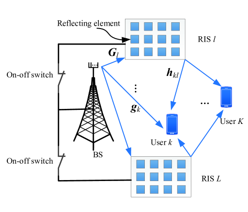
Figure 1: A downlink MISO system with multiple RISs.

Consider an RIS-assisted MISO downlink channel that consists of one BS, a set $\mathcal{K}$ of $K$ users, and a set $\mathcal{L}$ of $L$ RISs, as shown in Fig. 1. The number of transmit antennas at the BS is $M$, while each user is equipped with one antenna. Such a setting has been used in many practical scenarios such as in Internet-of-Things networks [18, 19, 20]. Each RIS, $l\in\mathcal{L}$, has $N_{l}$ reflecting elements. The RISs are configured to assist the communication between the BS and users. In particular, the RISs will be installed on the walls of the surrounding high-rise buildings.

The transmitted signal at the BS is:

$$\bm{s}=\sum_{k=1}^{K}\bm{w}_{k}s_{k},$$ (1)

where $s_{k}$ is unit-power information symbol [25] and $\bm{w}_{k}\in\mathbb{C}^{M}$ is the beamforming vector for user $k\in\mathcal{K}$.

The power consumption of an RIS depends on both the type and the resolution of the reflecting elements that effectively perform phase shifting on the impinging signal [25, 26, 27]. Considering the power consumption of RISs due to controlling the phase shift values of the reflecting elements [25], it is often not energy efficient to turn on all the RISs. We now introduce a binary variable $x_{l}\in\{0,1\}$, where $x_{l}=1$ indicates that RIS $l$ is on. When $x_{l}=1$, the phase shift matrix of RIS $l$ can be optimized through a diagonal matrix $\bm{\Theta}_{l}=\text{diag}(\text{e}^{j\theta_{l1}},\cdots,\text{e}^{j\theta_{lN_{l}}})\in\mathbb{C}^{N_{l}\times N_{l}}$ with $\theta_{ln}\in[0,2\pi]$, $l\in\mathcal{L}$, and $n\in\mathcal{N}_{l}=\{1,\cdots,N_{l}\}$, where $\bm{\Theta}_{l}$ captures the effective phase shifts applied by all reflecting elements of RIS $l$. In contrast, when $x_{l}=0$, RIS $l$ is off and does not consume any power. Then, with the multiple RISs, the received signal at user $k$ can be given by:

$$y_{k}=\left(\bm{g}_{k}^{H}+\sum_{l=1}^{L}x_{l}\bm{h}_{kl}^{H}\bm{\Theta}_{l}\bm{G}_{l}\right)\bm{s}+n_{k},$$ (2)

where $\bm{g}_{k}\in\mathbb{C}^{M}$, $\bm{G}_{l}\in\mathbb{C}^{N_{l}\times M}$, and $\bm{h}_{kl}\in\mathbb{C}^{N_{l}}$, respectively, denote the channel responses from the BS to user $k$, from the BS to RIS $l$, and from RIS $l$ to user $k$, and $n_{k}\sim\mathcal{CN}(0,\sigma^{2})$ is the additive white Gaussian noise.

Based on (1) and (2), the received signal-to-interference-plus-noise ratio (SINR) at user $k$ is:

$$\gamma_{k}=\frac{\left|\left(\bm{g}_{k}^{H}+\sum_{l=1}^{L}x_{l}\bm{h}_{kl}^{H}\bm{\Theta}_{l}\bm{G}_{l}\right)\bm{w}_{k}\right|^{2}}{\sum_{i=1,i\neq k}^{K}\left|\left(\bm{g}_{k}^{H}+\sum_{l=1}^{L}x_{l}\bm{h}_{kl}^{H}\bm{\Theta}_{l}\bm{G}_{l}\right)\bm{w}_{i}\right|^{2}+\sigma^{2}}.$$ (3)

As a result, the sum-rate of all users is:

$$R_{\text{t}}=B\sum_{k=1}^{K}\log_{2}(1+\gamma_{k}),$$ (4)

where $B$ is the bandwidth of the channel.

II-B Power Consumption Model

The total power consumption of the considered RIS-assisted system includes the transmit power of the BS, the circuit power consumption of both the BS and all users, and the power consumption of all RISs. Consequently, the total power of the system will be given by:

$$P_{\text{t}}=\underbrace{\sum_{k=1}^{K}\mu\bm{w}_{k}^{H}\bm{w}_{k}}_{\text{transmit power of the BS}}+\underbrace{P_{\text{B}}}_{\text{circuit power of the BS}}+\underbrace{\sum_{k=1}^{K}P_{k}}_{\text{circuit power of all users}}+\underbrace{\sum_{l=1}^{L}x_{l}N_{l}P_{\text{R}}}_{\text{power consumption of all RISs}},$$ (5)

where $\mu=\nu^{-1}$ with $\nu$ being the power amplifier efficiency of the BS, $P_{\text{B}}$ is the circuit power consumption of the BS, $P_{k}$ is the circuit power consumption of user $k$, and $P_{\text{R}}$ is the power consumption of each reflecting element in the RIS. In (5), $x_{l}N_{l}P_{\text{R}}$ is the power consumption of RIS $l$.

II-C Problem Formulation

Given the considered system model, our objective is to jointly optimize the reflection coefficients matrix, beamforming vector, and RIS on-off vector so as to maximize the energy efficiency under the minimum rate requirements and total power constraint. Mathematically, the problem for the distributed RISs can be given by:

$$\mathop{\max}_{\bm{\theta},\bm{w},\bm{x}}\quad \frac{R_{\text{t}}}{P_{\text{t}}}=\frac{B\sum_{k=1}^{K}\log_{2}\left(1+\frac{\left|\left(\bm{g}_{k}^{H}+\sum_{l=1}^{L}x_{l}\bm{h}_{kl}^{H}\bm{\Theta}_{l}\bm{G}_{l}\right)\bm{w}_{k}\right|^{2}}{\sum_{i=1,i\neq k}^{K}\left|\left(\bm{g}_{k}^{H}+\sum_{l=1}^{L}x_{l}\bm{h}_{kl}^{H}\bm{\Theta}_{l}\bm{G}_{l}\right)\bm{w}_{i}\right|^{2}+\sigma^{2}}\right)}{\mu\bm{w}^{H}\bm{w}+\sum_{k=1}^{K}P_{k}+P_{\text{B}}+\sum_{l=1}^{L}x_{l}N_{l}P_{\text{R}}}$$ (6)

s.t. $${B\log_{2}\left(1+\frac{\left|\left(\bm{g}_{k}^{H}+\sum_{l=1}^{L}x_{l}\bm{h}_{kl}^{H}\bm{\Theta}_{l}\bm{G}_{l}\right)\bm{w}_{k}\right|^{2}}{\sum_{i=1,i\neq k}^{K}\left|\left(\bm{g}_{k}^{H}+\sum_{l=1}^{L}x_{l}\bm{h}_{kl}^{H}\bm{\Theta}_{l}\bm{G}_{l}\right)\bm{w}_{i}\right|^{2}+\sigma^{2}}\right)}\geq R_{k},\quad\forall k\in\mathcal{K},$$ (6a)

$$\bm{w}^{H}\bm{w}\leq P_{\max},$$ (6b)

$$\theta_{ln}\in[0,2\pi],\quad\forall l\in\mathcal{L},n\in\mathcal{N}_{l},$$ (6c)

$$x_{l}\in\{0,1\},\quad\forall l\in\mathcal{L},$$ (6d)

where $\bm{\theta}=[\theta_{11},\cdots,\theta_{1N_{1}},\cdots,\theta_{LN_{L}}]^{T}$, $\bm{w}=[\bm{w}_{1};\cdots;\bm{w}_{K}]$, $\bm{x}=[x_{1},\cdots,x_{L}]^{T}$, $R_{k}$ is the minimum data rate requirement of user $k$, and $P_{\max}$ is the maximum transmit power of the BS. The minimum rate constraint for each user is given in (6a) and (6b) represents the total power constraint. The phase shift constraint for each reflecting element is provided in (6c), which can also be seen as the unit-modulus constraint since $|\text{e}^{j\theta_{ln}}|=1$. The problem in (6) is a mixed-integer nonlinear program (MINLP) even for the single-user case with $K=1$. It is generally difficult to obtain the globally optimal solution of the MINLP problem in (6). In the following, we propose two iterative algorithms to obtain suboptimal solutions of problem (6) for the single-user case and the multi-user case, respectively.

III Energy Efficiency Optimization with A Single User

In this section, we consider the single-user case, i.e., $K=1$. For $K=1$, problem (6) becomes:

$$\mathop{\max}_{\bm{\theta},\bm{w}_{1},\bm{x}}\quad \frac{B\log_{2}\left(1+\frac{\left|\left(\bm{g}_{1}^{H}+\sum_{l=1}^{L}x_{l}\bm{h}_{1l}^{H}\bm{\Theta}_{l}\bm{G}_{l}\right)\bm{w}_{1}\right|^{2}}{\sigma^{2}}\right)}{\mu\bm{w}_{1}^{H}\bm{w}_{1}+P_{1}+P_{\text{B}}+\sum_{l=1}^{L}x_{l}N_{l}P_{\text{R}}}$$ (7)

s.t. $${B\log_{2}\left(1+\frac{\left|\left(\bm{g}_{1}^{H}+\sum_{l=1}^{L}x_{l}\bm{h}_{1l}^{H}\bm{\Theta}_{l}\bm{G}_{l}\right)\bm{w}_{1}\right|^{2}}{\sigma^{2}}\right)}\geq R_{1},$$ (7a)

$$\bm{w}_{1}^{H}\bm{w}_{1}\leq P_{\max},$$ (7b)

$$\theta_{ln}\in[0,2\pi],\quad\forall l\in\mathcal{L},n\in\mathcal{N}_{l},$$ (7c)

$$x_{l}\in\{0,1\},\quad\forall l\in\mathcal{L}.$$ (7d)

Since there is no multi-user interference, it is well-known that beaming as the the maximum ratio transmission (MRT) at the BS is optimal [28]. That is:

$$\bm{w}_{1}=\sqrt{p_{1}}\frac{\bm{g}_{1}+\sum_{l=1}^{L}x_{l}\bm{G}_{l}^{H}\bm{\Theta}_{l}^{H}\bm{h}_{1l}}{|\bm{g}_{1}+\sum_{l=1}^{L}x_{l}\bm{G}_{l}^{H}\bm{\Theta}_{l}^{H}\bm{h}_{1l}|},$$ (8)

where $p_{1}\leq P_{\max}$ helps satisfy the transmit power constraint at the BS. Substituting the optimal beamforming in (8) into problem (7), it becomes:

$$\mathop{\max}_{\bm{\theta},p_{1},\bm{x}}\quad \frac{B\log_{2}\left(1+\frac{p_{1}\left|\bm{g}_{1}^{H}+\sum_{l=1}^{L}x_{l}\bm{h}_{1l}^{H}\bm{\Theta}_{l}\bm{G}_{l}\right|^{2}}{\sigma^{2}}\right)}{\mu p_{1}+P_{1}+P_{\text{B}}+\sum_{l=1}^{L}x_{l}N_{l}P_{\text{R}}}$$ (9)

s.t. $${B\log_{2}\left(1+\frac{p_{1}\left|\bm{g}_{1}^{H}+\sum_{l=1}^{L}x_{l}\bm{h}_{1l}^{H}\bm{\Theta}_{l}\bm{G}_{l}\right|^{2}}{\sigma^{2}}\right)}\geq R_{1},$$ (9a)

$$0\leq p_{1}\leq P_{\max},$$ (9b)

$$\theta_{ln}\in[0,2\pi],\quad\forall l\in\mathcal{L},n\in\mathcal{N}_{l},$$ (9c)

$$x_{l}\in\{0,1\},\quad\forall l\in\mathcal{L}.$$ (9d)

Due to the involvement of integer variable $\bm{x}$, it is difficult to obtain the globally optimal solution of (9). As such, we propose an iterative algorithm to solve problem (9) sub-optimally with low complexity. The proposed iterative algorithm contains two major steps. In the first step, we jointly optimize phase and power $(\bm{\theta},p_{1})$ with given $\bm{x}$. Then, in the second step, we update RIS on-off vector $\bm{x}$ with the optimized $(\bm{\theta},p_{1})$ in the previous step.

III-A Joint Phase and Power Optimization

For a fixed integer variable $\bm{x}$, problem (9) becomes:

$$\mathop{\max}_{\bm{\theta},p_{1}}\quad \frac{B\log_{2}\left(1+\frac{p_{1}\left|\bm{g}_{1}^{H}+\sum_{l=1}^{L}x_{l}\bm{h}_{1l}^{H}\bm{\Theta}_{l}\bm{G}_{l}\right|^{2}}{\sigma^{2}}\right)}{\mu p_{1}+P_{1}+P_{\text{B}}+\sum_{l=1}^{L}x_{l}N_{l}P_{\text{R}}}$$ (10)

s.t. $${B\log_{2}\left(1+\frac{p_{1}\left|\bm{g}_{1}^{H}+\sum_{l=1}^{L}x_{l}\bm{h}_{1l}^{H}\bm{\Theta}_{l}\bm{G}_{l}\right|^{2}}{\sigma^{2}}\right)}\geq R_{1},$$ (10a)

$$0\leq p_{1}\leq P_{\max},$$ (10b)

$$\theta_{ln}\in[0,2\pi],\quad\forall l\in\mathcal{L},n\in\mathcal{N}_{l}.$$ (10c)

From the objective function (10) and the constraint in (10a), we observe that the optimal $\bm{\theta}$ is the one that maximizes the channel gain, i.e., $\left|\left(\bm{g}_{1}^{H}+\sum_{l=1}^{L}x_{l}\bm{h}_{1l}^{H}\bm{\Theta}_{l}\bm{G}_{l}\right)\right|^{2}$. With this in mind, the optimal solution of problem (10) can be obtained in two stages, i.e., obtain the value of $\bm{\theta}$ that maximizes $\left|\left(\bm{g}_{1}^{H}+\sum_{l=1}^{L}x_{l}\bm{h}_{1l}^{H}\bm{\Theta}_{l}\bm{G}_{l}\right)\right|^{2}$ in the first stage and, then, calculate the optimal $p_{1}$ in the second stage with the obtained $\bm{\theta}$ in the first stage.

III-A1 First stage

We first optimize the phase shift vector $\bm{\theta}$ of problem (10). Before optimizing $\bm{\theta}$, we show that $\bm{h}_{1l}^{H}\bm{\Theta}_{l}\bm{G}_{l}=\bm{\theta}_{l}^{T}\bm{U}_{1l}$, where $\bm{U}_{1l}=\text{diag}(\bm{h}_{1l}^{H})\bm{G}_{l}\in\mathbb{C}^{N_{l}\times M}$ and $\bm{\theta}_{l}=[\text{e}^{j\theta_{l1}},\cdots,\text{e}^{j\theta_{lN_{l}}}]^{T}$. According to problem (10), the optimal $\bm{\theta}$ can be calculated by solving the following problem:

$$\mathop{\max}_{\bm{\theta}}\quad \left|\bm{g}_{1}^{H}+\sum_{l=1}^{L}x_{l}\bm{\theta}_{l}^{T}\bm{U}_{1l}\right|^{2}$$ (11)

s.t. $$\theta_{ln}\in[0,2\pi],\quad\forall l\in\mathcal{L},n\in\mathcal{N}_{l}.$$ (11a)

Let $\bm{\theta}_{l}^{*}$ be the conjugate vector of $\bm{\theta}_{l}$. The total number of elements for all RISs is denoted by $Q=\sum_{l=1}^{L}N_{l}$. Denote $\bm{v}=[\bm{\theta}_{1}^{*};\cdots;\bm{\theta}_{L}^{*}]\in\mathbb{C}^{Q}$ and $\bm{U}_{1}=[x_{1}\bm{U}_{1l};\cdots;x_{L}\bm{U}_{1L}]\in\mathbb{C}^{Q\times M}$. Problem (11) can be rewritten as:

$$\mathop{\max}_{{\bm{v}}}\quad \left|{\bm{g}}_{1}+{\bm{U}}_{1}^{H}{\bm{v}}\right|^{2}$$ (12)

s.t. $$|v_{q}|=1,\quad\forall q\in\mathcal{Q},$$ (12a)

where $\mathcal{Q}=\{1,\cdots,Q\}$.

To solve the optimization problem in (12), various methods were proposed by techniques such as semidefinite relaxation (SDR) technique [29] and successive refinement (SR) algorithm [30]. However, the SDR method imposes high complexity to obtain a rank-one solution and the SR algorithm requires a large number of iterations due to the need for updating the phase shifts in a one-by-one manner. To reduce the computational complexity, we propose the SCA method to solve the phase shift optimization problem (12).

To handle the nonconvexity of objective function (12), we adopt the SCA method and, consequently, objective function (12) can be approximated by:

$$\quad 2\mathcal{R}(({\bm{g}}_{1}+{\bm{U}}_{1}^{H}{\bm{v}}^{(n-1)})^{H}{\bm{U}}_{1}^{H}{\bm{v}})-\left|{\bm{g}}_{1}+{\bm{U}}_{1}^{H}{\bm{v}}^{(n-1)}\right|^{2},$$ (13)

which is the first-order Taylor series of $\left|{\bm{g}}_{1}+{\bm{U}}_{1}^{H}{\bm{v}}\right|^{2}$ and the superscript $(n-1)$ represents the value of the variable at the $(n-1)$-th iteration.

With the above approximation (13), the nonconvex problem (12) can be approximated by the following convex problem:

$$\mathop{\max}_{{\bm{v}}}\quad 2\mathcal{R}(({\bm{g}}_{1}+{\bm{U}}_{1}^{H}{\bm{v}}^{(n-1)})^{H}{\bm{U}}_{1}^{H}{\bm{v}})-\left|{\bm{g}}_{1}+{\bm{U}}_{1}^{H}{\bm{v}}^{(n-1)}\right|^{2}$$ (14)

s.t. $$|v_{q}|\leq 1,\quad\forall q\in\mathcal{Q},$$ (14a)

where constraint (12a) is temporarily relaxed as (14a). In the following lemma, we show that (14a) always holds with equality for the optimal solution of problem (14).

Lemma 1

The optimal solution of problem (14) is:

$$\bm{v}=\text{e}^{-j\angle({\bm{U}}_{1}({\bm{g}}_{1}+{\bm{U}}_{1}^{H}{\bm{v}}^{(n-1)}))},$$ (15)

where $\angle(\cdot)$ represents the angle vector of a vector, i.e, $[\angle(\bm{y})]_{q}=\arctan\frac{\mathcal{I}([\bm{y}]_{q})}{\mathcal{R}([\bm{y}]_{q})}$.

Proof: To maximize $({\bm{g}}_{1}+{\bm{U}}_{1}^{H}{\bm{v}}^{(n-1)})^{H}{\bm{U}}_{1}^{H}{\bm{v}}$ in (14), the optimal $\bm{v}$ should be chosen such that $[({\bm{g}}_{1}+{\bm{U}}_{1}^{H}{\bm{v}}^{(n-1)})^{H}{\bm{U}}_{1}^{H}]_{q}[{\bm{v}}]_{q}$ is a real number and $|[{\bm{v}}]_{q}|=1$ for any $q$, i.e., the optimal $\bm{v}$ should be given as (15). $\Box$

From (15) and Lemma 1, we can see that the optimal phase vector $\bm{v}$ should be adjusted such that the signal that goes through all RISs is aligned to be a signal vector with equal phase at each element. We can also see that the optimal phase vector $\bm{v}$ is independent of the amplitude of the channel ${\bm{U}}_{1}({\bm{g}}_{1}+{\bm{U}}_{1}^{H}{\bm{v}}^{(n-1)})$.

Algorithm 1 SCA Method for Phase Optimization

1:  Initialize $\bm{v}^{(0)}$. Set iteration number $n=1$.

2:  repeat

3:     Set $\bm{v}^{(n)}=\text{e}^{-j\angle({\bm{U}}_{1}({\bm{g}}_{1}+{\bm{U}}_{1}^{H}{\bm{v}}^{(n-1)}))},$ and $n=n+1$.

4:  until the objective value (12) converges.

5:  Output $\bm{\theta}=(\bm{v}^{(n)})^{*}$.

The SCA algorithm for solving problem (12) is summarized in Algorithm 1. The convergence of Algorithm 1 is guaranteed by the following lemma that follows directly from [31, Proposition 3]:

Lemma 2

The objective value (12) obtained in Algorithm 1 is monotonically non-decreasing and the sequence $\bm{v}^{(n)}$ converges to a point fulfilling the Karush-Kuhn-Tucker (KKT) optimal conditions of the original nonconvex problem (12).

Lemma 2 shows that Algorithm 1 will always converge to a locally optimal solution of problem (12).

III-A2 Second stage

We now obtain the optimal power allocation $p_{1}$. With the obtained ${\bm{\theta}}$ in Algorithm 1 and defining $\bar{g}_{1}=\frac{\left|\bm{g}_{1}^{H}+\sum_{l=1}^{L}x_{l}\bm{h}_{1l}^{H}\bm{\Theta}_{l}\bm{G}_{l}\right|^{2}}{\sigma^{2}}$, problem (10) reduces to:

$$\mathop{\max}_{p_{1}}\quad \frac{B\log_{2}\left(1+\bar{g}_{1}p_{1}\right)}{\mu p_{1}+P_{0}}$$ (16)

s.t. $$P_{\min}\leq p_{1}\leq P_{\max},$$ (16a)

where $P_{0}=P_{1}+P_{\text{B }}+\sum_{l=1}^{L}x_{l}N_{l}P_{\text{R}}$, and $P_{\min}=\frac{\left(2^{\frac{R_{1}}{B}}-1\right)}{\bar{g}_{1}}$. In (16a), $P_{\min}$ is used to guarantee the minimum rate requirement for user 1.

For the energy efficiency optimization problem (16), the Dinkelbach method from [32] can be used. The Dinkelbach method involves solving a series of convex subproblems, which increases the computational complexity. However, the optimal solution of (16) can be derived in closed form using the following theorem.

Theorem 1

The optimal transmit power of the energy efficiency maximization problem in (16) is:

$$p_{1}=\left[\frac{\bar{g}_{1}P_{0}-\mu}{\mu\bar{g}_{1}W\left(\frac{(\bar{g}_{1}P_{0}-\mu)}{\mu\text{e}}\right)}-\frac{1}{\bar{g}_{1}}\right]_{P_{\min}}^{P_{\max}},$$ (17)

where $W(\cdot)$ is the Lambert-W function and $[a]_{b}^{c}=\min\{\max\{a,b\},c\}$.

Proof: The first-order derivative of the objective function (16) with respect to power $p_{1}$ is:

$$\frac{\partial\frac{B\log_{2}(1+\bar{g}_{1}p_{1})}{\mu p_{1}+P_{0}}}{\partial p_{1}}=\frac{B({\bar{g}_{1}}(\mu p_{1}+P_{0})-\mu(1+\bar{g}_{1}p_{1})\ln(1+\bar{g}_{1}p_{1}))}{(1+\bar{g}_{1}p_{1})(\mu p_{1}+P_{0})^{2}\ln 2}.$$ (18)

To show the increasing trend of the objective function (16), we further denote:

$$f_{1}(p_{1})=\bar{g}_{1}(\mu p_{1}+P_{0})-\mu(1+\bar{g}_{1}p_{1})\ln(1+\bar{g}_{1}p_{1}),\quad\forall p_{1}>0.$$ (19)

The first-order derivative of function $f_{1}(p_{1})$ is:

$$f_{1}^{\prime}(p_{1})=-\mu\bar{g}_{1}\ln(1+\bar{g}_{1}p_{1})<0,$$ (20)

which indicates that $f_{1}(p_{1})$ is a monotonically decreasing function. Since $f_{1}(0)=\bar{g}_{1}P_{0}>0$ and $\lim_{p_{1}\rightarrow\infty}f_{1}(p_{1})<0$, there must exist a unique $\bar{p}_{1}$ such that $f_{1}(\bar{p}_{1})=0$, where

$$\bar{p}_{1}=\frac{\bar{g}_{1}P_{0}-\mu}{\mu\bar{g}_{1}W\left(\frac{(\bar{g}_{1}P_{0}-\mu)}{\mu\text{e}}\right)}-\frac{1}{\bar{g}_{1}}.$$ (21)

Hence, the objective function (16) first increases in interval $(0,\bar{p}_{1}]$ and then decreases in interval $(\bar{p}_{1},\infty)$, which indicates that the optimal solution can be presented as in (17). $\Box$

From Theorem 1, the optimal power control of problem (16) is obtained in closed-form, as shown in (17). According to (17), it is shown that the optimal power control lies in one of three values, i.e., the minimum transmit power, the power with zero first-order derivative, and the maximum transmit power.

III-B RIS On-Off Optimization

Substituting the phase and power variables $(\bm{\theta},p_{1})$ obtained in the previous section, problem (9) becomes:

$$\mathop{\max}_{\bm{x}}\quad \frac{B\log_{2}\left(1+\frac{p_{1}\left|\bm{g}_{1}^{H}+\sum_{l=1}^{L}x_{l}\bm{h}_{1l}^{H}\bm{\Theta}_{l}\bm{G}_{l}\right|^{2}}{\sigma^{2}}\right)}{\mu p_{1}+P_{1}+P_{\text{B}}+\sum_{l=1}^{L}x_{l}N_{l}P_{\text{R}}}$$ (22)

s.t. $${B\log_{2}\left(1+\frac{p_{1}\left|\bm{g}_{1}^{H}+\sum_{l=1}^{L}x_{l}\bm{h}_{1l}^{H}\bm{\Theta}_{l}\bm{G}_{l}\right|^{2}}{\sigma^{2}}\right)}\geq R_{1},$$ (22a)

$$x_{l}\in\{0,1\},\quad\forall l\in\mathcal{L}.$$ (22b)

We introduce an auxiliary variable $y$ and problem (22) is equivalent to:

$$\mathop{\max}_{\bm{x},y}\quad \frac{B\log_{2}\left(1+\frac{p_{1}y}{\sigma^{2}}\right)}{\mu p_{1}+P_{1}+P_{\text{B}}+\sum_{l=1}^{L}x_{l}N_{l}P_{\text{R}}}$$ (23)

s.t. $$y\leq{\left|\bm{g}_{1}^{H}+\sum_{l=1}^{L}x_{l}\bm{h}_{1l}^{H}\bm{\Theta}_{l}\bm{G}_{l}\right|^{2}},$$ (23a)

$$y\geq\left(2^{\frac{R_{1}}{B}}-1\right)\frac{\sigma^{2}}{p_{1}},$$ (23b)

$$x_{l}\in\{0,1\},\quad\forall l\in\mathcal{L},$$ (23c)

where constraint (23b) is used to ensure the minimum rate demand. For the optimal solution of problem (23), constraint (23a) will always hold with equality since the objective function monotonically increases with $y$. Although problem (23) has a simplifier form compared to (22), it is still a nonconvex MINLP. There are two difficulties in solving problem (23). The first difficulty is that objective function (23) has a fractional form, which is difficult to solve. The second difficulty is that constraint (23a) is nonconvex.

To handle the first difficulty, we use the parametric approach in [32] and consider the following problem:

$$H(\lambda)=\mathop{\max}_{(\bm{x},y)\in\mathcal{F}}{B\log_{2}\left(1+\frac{p_{1}y}{\sigma^{2}}\right)}-\lambda\left({\mu p_{1}+P_{1}+P_{\text{B}}+\sum_{l=1}^{L}x_{l}N_{l}P_{\text{R}}}\right),$$ (24)

where $\mathcal{F}$ is the feasible set of $(\bm{x},y)$ satisfying constraints (23a)-(23c). It was proved in [32] that solving (23) is equivalent to finding the root of the nonlinear function $H(\lambda)$, which can be obtained by using the Dinkelbach method. By introducing parameter $\lambda$, the objective function of problem (23) can be simplified, as shown in (24).

To handle the second difficulty, due to the fact that $x_{l}\in\{0,1\}$, we can rewrite the right hand side of constraint (23a) as:

$$\left|\bm{g}_{1}^{H}+\sum_{l=1}^{L}x_{l}\bm{h}_{1l}^{H}\bm{\Theta}_{l}\bm{G}_{l}\right|^{2}=D_{0}+\sum_{l=1}^{L}D_{l}x_{l}+\sum_{l=2}^{L}\sum_{m=1}^{l-1}D_{lm}x_{l}x_{m},$$ (25)

where $D_{0}=\bm{g}_{1}^{H}\bm{g}_{1}$, $D_{l}=\bm{h}_{1l}^{H}\bm{\Theta}_{l}\bm{G}_{l}\bm{G}_{l}^{H}\bm{\Theta}_{l}^{H}\bm{h}_{1l}+\bm{g}_{1}^{H}\bm{G}_{l}^{H}\bm{\Theta}_{l}^{H}\bm{h}_{1l}+\bm{h}_{1l}^{H}\bm{\Theta}_{l}\bm{G}_{l}\bm{g}_{1}$, and $D_{lm}=\bm{h}_{1l}^{H}\bm{\Theta}_{l}\bm{G}_{l}\bm{G}_{m}^{H}\bm{\Theta}_{m}^{H}\bm{h}_{1m}+\bm{h}_{1m}^{H}\bm{\Theta}_{m}\bm{G}_{m}\bm{G}_{l}^{H}\bm{\Theta}_{l}^{H}\bm{h}_{1l}$. To solve problem (23), we introduce new variable $z_{lm}=x_{l}x_{m}$. Since $x_{l}\in\{0,1\}$, constraint $z_{lm}=x_{l}x_{m}$ is equivalent to:

$$z_{lm}\geq x_{l}+x_{m}-1,\quad 0\leq z_{lm}\leq 1,$$ (26)

$$z_{lm}\leq x_{l},\quad z_{lm}\leq x_{m},$$ (27)

for all $l=2,\cdots,L$, $m=1,\cdots,l-1$. According to (24)-(27), problem (23) can be reformulated as:

$$\mathop{\max}_{\bm{x},y,\bm{z}}\quad {B\log_{2}\left(1+\frac{p_{1}y}{\sigma^{2}}\right)}-\lambda\left({\mu p_{1}+P_{1}+P_{\text{B}}+\sum_{l=1}^{L}x_{l}N_{l}P_{\text{R}}}\right)$$ (28)

s.t. $$y\leq D_{0}+\sum_{l=1}^{L}D_{l}x_{l}+\sum_{l=2}^{L}\sum_{m=1}^{l-1}D_{lm}z_{lm},$$ (28a)

$$z_{lm}\geq x_{l}+x_{m}-1,z_{lm}\leq x_{l},z_{lm}\leq x_{m},\quad\forall l=2,\cdots,L,m=1,\cdots,l-1,$$ (28b)

$$y\geq\left(2^{\frac{R_{1}}{B}}-1\right)\frac{\sigma^{2}}{p_{1}},$$ (28c)

$$0\leq z_{lm}\leq 1,\quad\forall l=2,\cdots,L,m=1,\cdots,l-1,$$ (28d)

$$x_{l}\in\{0,1\},\quad\forall l\in\mathcal{L},$$ (28e)

where $\bm{z}=[z_{21},z_{31},z_{32},\cdots,z_{L(L-1)}]^{T}$.

Due to constraints (28e), it is difficult to handle problem (28). By relaxing the integer constraints (28e) with $x_{l}\in[0,1]$, problem (28) becomes a convex problem. For problem (28) with relaxed constraints, the optimal solution can be obtained through the dual method [33]. We show that the dual method obtains the integer solution, which guarantees both optimality and feasibility of the original problem. To obtain the optimal solution of problem (28), we have the following theorem.

Theorem 2

For problem (28), the optimal RIS on-off vector $\bm{x}$ and auxiliary variables $(y,\bm{z})$ can be respectively expressed as:

$$x_{l}=\left\{\begin{array}[]{ll}\!\!1,&\text{if}\;C_{l}>0,\\ \!\!0,&\text{otherwise},\end{array}\right.$$ (29)

$$y=\left.\left(\frac{B}{(\ln 2)\alpha}-\frac{\sigma^{2}}{p_{1}}\right)\right|_{\left(2^{\frac{R_{1}}{B}}-1\right)\frac{\sigma^{2}}{p_{1}}},$$ (30)

and

$$z_{lm}=\left\{\begin{array}[]{ll}\!\!1,&\text{if}\;\alpha D_{lm}+\kappa_{1lm}-\kappa_{2lm}-\kappa_{3lm}>0,\\ \!\!0,&\text{otherwise},\end{array}\right.$$ (31)

where

$$C_{l}\!=\!\left\{\begin{array}[]{l}\!\!\!-\lambda N_{1}P_{\text{R}}+\alpha D_{1}+\sum_{m=2}^{L}(\kappa_{3ml}-\kappa_{1ml}),\quad\text{if}\;l=1,\\ \!\!\!-\lambda N_{l}P_{\text{R}}+\alpha D_{l}+\sum_{m=1}^{l-1}(\kappa_{2lm}-\kappa_{1lm})+\sum_{m=l+1}^{L}(\kappa_{3ml}-\kappa_{1ml}),\quad\text{if}\;2\leq l\leq L-1,\\ \!\!\!-\lambda N_{L}P_{\text{R}}+\alpha D_{L}+\sum_{m=1}^{L-1}(\kappa_{2lm}-\kappa_{1lm}),\quad\text{if}\;l=L,\end{array}\right.$$ (32)

$\{\alpha,\kappa_{1lm},\kappa_{2lm},\kappa_{3lm}\}$ are the Lagrange multipliers associated with corresponding constraints of problem (28), and $a_{b}=\max\{a,b\}$.

Proof: The dual problem of problem (28) with relaxed constraints is:

$$\mathop{\min}_{\alpha,\bm{\kappa}}\quad\mathcal{D}(\alpha,\bm{\kappa}),$$ (33)

where

$$\mathcal{D}(\alpha,\bm{\kappa})=\left\{\begin{array}[]{ll}\!\!\!\mathop{\max}\limits_{\bm{x},y,\bm{z}}&\mathcal{L}(\bm{x},y,\bm{z},\alpha,\bm{\kappa})\\ \!\!\rm{s.t.}&y\geq\left(2^{\frac{R_{1}}{B}}-1\right)\frac{\sigma^{2}}{p_{1}},\\ &0\leq z_{lm}\leq 1,\quad\forall l=2,\cdots,L,m=1,\cdots,l-1,\\ &0\leq x_{l}\leq 1,\quad\forall l\in\mathcal{L},\end{array}\right.$$ (34)

$$\mathcal{L}(\bm{x},y, \bm{z},\alpha,\bm{\kappa})={B\log_{2}\left(1+\frac{p_{1}y}{\sigma^{2}}\right)}-\lambda\left({\mu p_{1}+P_{1}+P_{\text{B}}+\sum_{l=1}^{L}x_{l}N_{l}P_{\text{R}}}\right)$$

$$+\alpha\left(D_{0}+\sum_{l=1}^{L}D_{l}x_{l}+\sum_{l=2}^{L}\sum_{m=1}^{l-1}D_{lm}z_{lm}-y\right)$$

$$+\sum_{l=2}^{L}\sum_{m=1}^{l-1}\left[\kappa_{1lm}(z_{lm}-x_{l}-x_{m}+1)+\kappa_{2lm}(x_{l}-z_{lm})+\kappa_{3lm}(x_{m}-z_{lm})\right],$$ (35)

and $\bm{\kappa}=\{\kappa_{1lm},\kappa_{2lm},\kappa_{3lm}\}_{l=2,\cdots,L,m=1,\cdots,l-1}$.

To maximize the objective function in (34), which is a linear combination of $x_{l}$ and $z_{lm}$, we must let the positive coefficients corresponding to the $x_{l}$ and $z_{lm}$ be 1. Therefore, the optimal $x_{l}$ and $z_{lm}$ are thus given as (29) and (31), respectively.

To optimize $y$ from (34), we set the first derivative of objective function to zero, i.e.,

$$\frac{\partial\mathcal{L}(\bm{x},y,\bm{z},\alpha,\bm{\kappa})}{\partial y}=\frac{Bp_{1}}{(p_{1}y+\sigma^{2})\ln 2}-\alpha=0,$$ (36)

which yields $y=\frac{B}{(\ln 2)\alpha}-\frac{\sigma^{2}}{p_{1}}$. Considering constraint (28c), we obtain the optimal solution to problem (28) as (30). $\Box$

Theorem 2 states that RIS $l$ that has a positive coefficient $C_{l}$ should be on. According to the expression of coefficient $C_{l}$ in (32), the negative term $-\lambda N_{l}P_{\text{R}}$, is the effect of introducing additional power consumption if RIS $l$ is on, while the remaining term represents the benefit of increasing the transmit rate by keeping RIS $l$ in operation. When $C_{l}>0$, the benefit of increasing the transmit rate is larger than the effect of introducing additional power consumption, which means that the energy efficiency can be improved if RIS $l$ is on.

The values of $(\alpha,\bm{\kappa})$ are determined by the sub-gradient method [34, 35, 36, 37], which can be given by

$$\!\!\!\!\!\!\!\!\!\!\!\!\!\!\!\!\!\!\alpha=\left[\alpha-\phi\left(D_{0}+\sum_{l=1}^{L}D_{l}x_{l}+\sum_{l=2}^{L}\sum_{m=1}^{l-1}D_{lm}z_{lm}-y\right)\right]^{+},$$ (37)

$$\!\!\!\!\!\!\!\!\!\!\!\!\!\!\!\!\!\!\kappa_{1lm}=[\kappa_{1lm}-\phi(z_{lm}-x_{l}-x_{m}+1)]^{+},$$ (38)

$$\!\!\!\!\!\!\!\!\!\!\!\!\!\!\!\!\!\!\kappa_{2lm}=\left[\kappa_{2lm}-\phi(x_{l}-z_{lm})\right]^{+},$$ (39)

$$\!\!\!\!\!\!\!\!\!\!\!\!\!\!\!\!\!\!\kappa_{3lm}=\left[\kappa_{3lm}-\phi(x_{m}-z_{lm})\right]^{+},$$ (40)

where $\phi>0$ is a dynamically chosen step-size sequence and $[a]^{+}=\max(a,0)$.

Algorithm 2 Dual Method for Problem (23)

1:  Initialize parameter $\lambda$ and set the accuracy $\epsilon$.

2:  repeat

3:     Initialize dual variables $(\alpha,\bm{\kappa})$.

4:     repeat

5:        Update the RIS on-off vector $\bm{x}$ and the auxiliary variables $(y,\bm{z})$ according to (29)-(31).

6:        Update dual variables $(\alpha,\bm{\kappa})$ based on (37)-(40).

7:     until the objective value (28) converges

8:     Denote the objective value (28) by $H(\lambda)$.

9:     Update $\lambda=\frac{B\log_{2}\left(1+\frac{p_{1}y}{\sigma^{2}}\right)}{\mu p_{1}+P_{1}+P_{\text{B}}+\sum_{l=1}^{L}x_{l}N_{l}P_{\text{R}}}$.

10:  until $H(\lambda)<\epsilon$.

By iteratively optimizing primal variables $(\bm{x},y,\bm{z})$ and dual variables $(\alpha,\bm{\kappa})$, the optimal RIS on-off vector is obtained. The dual method for solving problem (28) and the Dinkelbach method to update parameter $\lambda$ are given in Algorithm 2. Notice that the optimal $x_{l}$ is either 0 or 1 according to (29), even though we relax $x_{l}$ as (34). Consequently, the optimal solution to problem (28) is obtained by using the dual method, i.e., $H(\lambda)$ in (24) is obtained for given $\lambda$. Using the Dinkelbach method, we can obtain the root of $H(\lambda)=0$, which indicates that the optimal solution of fractional energy efficiency optimization problem (23) is obtained.

III-C Complexity Analysis

Algorithm 3 Iterative Optimization for Problem (9)

1:  Initialize $(\bm{\theta}^{(0)},p_{1}^{(0)},\bm{x}^{(0)})$. Set iteration number $n=1$.

2:  repeat

3:     Given $\bm{x}^{(n-1)}$, solve the phase optimization problem (12) by using Algorithm 1 and the solution is denoted by $\bm{\theta}^{(n)}$.

4:     Given $\bm{x}^{(n-1)}$ and the optimized $\bm{\theta}^{(n)}$, solve the power control problem (16) according to Theorem 1 and the optimal power is denoted by $p_{1}^{(n)}$.

5:     Given $(\bm{\theta}^{(n)},p_{1}^{(n)})$, solve the RIS on-off optimization problem (23) by using Algorithm 2 and the solution is denoted by $\bm{x}^{(n)}$.

6:     Set $n=n+1$.

7:  until the objective value (9) converges.

The iterative algorithm for solving problem (9) is given in Algorithm 3. From Algorithm 3, the main complexity of solving problem (9) lies in solving the phase optimization problem (12) and the RIS on-off optimization problem (23).

According to Algorithm 1, to solve the phase optimization problem (12), the complexity lies in computing $\bm{v}^{(n)}=\text{e}^{-j\angle({\bm{U}}_{1}({\bm{g}}_{1}+{\bm{U}}_{1}^{H}{\bm{v}}^{(n-1)}))}$ at each iteration, which involves the complexity of $\mathcal{O}(QM)$. Hence, the total complexity of solving problem (12) with Algorithm 1 is $\mathcal{O}(T_{1}QM)$, where $T_{1}$ is the total number of the iterations of Algorithm 1.

According to Algorithm 2, the main complexity of solving problem (23) lies in solving RIS on-off vector $\bm{x}$, which involves the complexity of $\mathcal{O}(L^{2})$ based on (29) and (32). Hence, the complexity of solving problem (23) with Algorithm 2 is $\mathcal{O}(T_{2}T_{3}L^{2})$, where $T_{2}$ is the number of inner iterations by updating primal variables and dual variables and $T_{3}$ is the number of inner iterations by updating the parameter $\lambda$.

As a result, the total complexity of solving problem (9) is $\mathcal{O}(T_{0}T_{1}QM+T_{0}T_{2}T_{3}L^{2})$, where $T_{0}$ is the total number of iterations for Algorithm 3. The complexity of the proposed Algorithm 3 grows quadratically with the number of all RISs and this complexity is lower than that of the SDR-based algorithm in [29].

IV Energy Efficiency Optimization with Multiple Users

In this section, we consider a general case with multiple users. To solve the energy efficiency optimization problem in (6), an iterative algorithm with low complexity is proposed via alternatingly optimizing the phase vector, beamforming vector, and RIS on-off vector.

IV-A Phase Optimization

Given beamforming vector $\bm{w}$ and RIS on-off vector $\bm{x}$, the total power consumption of the system is fixed and the energy efficiency maximization is equivalent to the sum-rate maximization. Thus, given $(\bm{w},\bm{x})$, problem (6) reduces to:

$$\mathop{\max}_{\bm{\theta},\bm{\eta}}\quad \sum_{k=1}^{K}\log_{2}\left(1+\eta_{k}\right)$$ (41)

s.t. $$\eta_{k}\leq\frac{\left|\left(\bm{g}_{k}^{H}+\sum_{l=1}^{L}x_{l}\bm{h}_{kl}^{H}\bm{\Theta}_{l}\bm{G}_{l}\right)\bm{w}_{k}\right|^{2}}{\sum_{i=1,i\neq k}^{K}\left|\left(\bm{g}_{k}^{H}+\sum_{l=1}^{L}x_{l}\bm{h}_{kl}^{H}\bm{\Theta}_{l}\bm{G}_{l}\right)\bm{w}_{i}\right|^{2}+\sigma^{2}},\quad\forall k\in\mathcal{K},$$ (41a)

$$\eta_{k}\geq 2^{\frac{R_{k}}{B}}-1,\quad\forall k\in\mathcal{K},$$ (41b)

$$\theta_{ln}\in[0,2\pi],\quad\forall l\in\mathcal{L},n\in\mathcal{N}_{l},$$ (41c)

where $\bm{\eta}=[\eta_{1},\cdots,\eta_{K}]^{T}$. In (41), $\bm{\eta}$ is a slack vector, which ensures that constraint (41a) always holds with equality for the optimal solution. Constraint (41b) is added to guarantee the minimum rate requirement of each user.

Before optimizing $\bm{\theta}$, we denote $s_{ln}=\text{e}^{j\theta_{ln}},\forall l\in\mathcal{L},n\in\mathcal{N}_{l}$, $\bm{s}_{l}=[s_{l1},\cdots,s_{lN_{l}}]^{T}$, and $\bm{s}=[s_{11},\cdots,s_{1N_{1}},\cdots,s_{LN_{L}}]^{T}$. With the help of $\bm{s}_{l}$, we show $\bm{h}_{kl}^{H}\bm{\Theta}_{l}\bm{G}_{l}\bm{w}_{i}=\bm{t}_{kli}^{H}\bm{s}_{l}$, where $\bm{t}_{kli}=(\text{diag}(\bm{h}_{kl}^{H})\bm{G}_{l}\bm{w}_{i})^{*}\in\mathbb{C}^{N_{l}}$. Hence, constraint (41a) can be rewritten as:

$$\eta_{k}\leq\frac{\left|{\bm{t}}_{kk}^{H}{\bm{s}}+\bar{g}_{kk}\right|^{2}}{\sum_{i=1,i\neq k}^{K}\left|{\bm{t}}_{ki}^{H}{\bm{s}}+\bar{g}_{ki}\right|^{2}+\sigma^{2}},\quad\forall k\in\mathcal{K},$$ (42)

where ${\bm{t}}_{ki}=[{\bm{t}}_{kl1};\cdots;{\bm{t}}_{klL}]$, $\bar{g}_{kk}={\bm{g}}_{k}^{H}\bm{w}_{k}$, and $\bar{g}_{ki}={\bm{g}}_{k}^{H}\bm{w}_{i}$.

Problem (41) can be reformulated as:

$$\mathop{\max}_{\bm{s},\bm{\eta}}\quad \sum_{k=1}^{K}\log_{2}\left(1+\eta_{k}\right)$$ (43)

s.t. $$|s_{ln}|=1,\quad\forall l\in\mathcal{L},n\in\mathcal{N}_{l},$$ (43a)

$$(\ref{eemumax1eq0}),(\ref{eemumax1}b).$$ (43b)

To handle the nonconvexity constraint (43a), we use the penalty method and problem (43) can be rewritten as:

$$\mathop{\max}_{\bm{s},\bm{\eta}}\quad \sum_{k=1}^{K}\log_{2}\left(1+\eta_{k}\right)+C\sum_{l=1}^{L}\sum_{n=1}^{N_{l}}(|s_{ln}|^{2}-1)$$ (44)

s.t. $$|s_{ln}|\leq 1,\quad\forall l\in\mathcal{L},n\in\mathcal{N}_{l},$$ (44a)

$$(\ref{eemumax1eq0}),(\ref{eemumax1}b),$$ (44b)

where $C$ is a large positive constant. Note that the penalty part $C\sum_{l=1}^{L}\sum_{n=1}^{N_{l}}(|s_{ln}|^{2}-1)$ enforces that $|s_{ln}|^{2}-1=0$ for the optimal solution of (44). To solve the nonconvex problem in (44), we utilize the SCA method. The objective function of (44) can be approximated by:

$$\sum_{k=1}^{K}\log_{2}\left(1+\eta_{k}\right)+2C\sum_{l=1}^{L}\sum_{n=1}^{N_{l}}s_{ln}^{(n-1)}(s_{ln}-s_{ln}^{(n-1)}),$$ (45)

where the second part is the first-order Taylor series of $C\sum_{l=1}^{L}\sum_{n=1}^{N_{l}}(|s_{ln}|^{2}-1)$ and the superscript $(n-1)$ means the value of the variable at the $(n-1)$-th iteration. To handle the nonconvexity of constraint (42), we introduce variable $\beta_{k}$ and constraint (42) is equivalent to:

$${\left|{\bm{t}}_{kk}^{H}{\bm{s}}+\bar{g}_{kk}\right|^{2}}\geq\beta_{k}\eta_{k}=\frac{1}{4}((\beta_{k}+\eta_{k})^{2}-(\beta_{k}-\eta_{k})^{2}),$$ (46)

and

$${\sum_{i=1,i\neq k}^{K}\left|{\bm{t}}_{ki}^{H}{\bm{s}}+\bar{g}_{ki}\right|^{2}+\sigma^{2}}\leq\beta_{k},$$ (47)

where (47) is convex, while it remains to handle the nonconvexity of (46). We adopt an approximation of the difference of two convex functions (DC) and constraint (46) can be approximated by:

$$\quad 2\mathcal{R}(({\bm{t}}_{kk}^{H}{\bm{s}}^{(n-1)}+\bar{g}_{kk})^{H}{\bm{t}}_{kk}^{H}{\bm{s}})-{\left|{\bm{t}}_{kk}^{H}{\bm{s}}^{(n-1)}+\bar{g}_{kk}\right|^{2}}$$

$$\geq\frac{1}{4}((\beta_{k}+\eta_{k})^{2}-(\beta_{k}^{(n-1)}-\eta_{k}^{(n-1)})(\beta_{k}-\eta_{k})+(\beta_{k}^{(n-1)}-\eta_{k}^{(n-1)})^{2}),$$ (48)

where the left hand side is the first-order Taylor expansion of ${\left|{\bm{t}}_{kk}^{H}{\bm{s}}+\bar{g}_{kk}\right|^{2}}$ with respect to $\bm{s}$ at $\bm{s}=\bm{s}^{(n-1)}$.

With the above approximations, the nonconvex problem in (44) can be formulated in the following approximated convex problem:

$$\mathop{\max}_{{\bm{s}},\bm{\eta},\bm{\beta}}\quad \sum_{k=1}^{K}\log_{2}\left(1+\eta_{k}\right)+2C\sum_{l=1}^{L}\sum_{n=1}^{N_{l}}s_{ln}^{(n-1)}(s_{ln}-s_{ln}^{(n-1)}),$$ (49)

s.t. $$\beta_{k}\geq 0,\quad\forall k\in\mathcal{K}$$ (49a)

$$(\ref{eemumax1eq1_2}),(\ref{eemumax1eq1_3}),(\ref{eemumax01}a),$$ (49b)

where $\bm{\beta}=[\beta_{1},\cdots,\beta_{K}]^{T}$. Problem (41) can be solved by using the SCA method, where the approximated convex problem (49) is solved at each iteration. The detailed process of using the SCA method to solve problem (41) is analogous to Algorithm 1.

IV-B Beamforming Optimization

Given phase vector $\bm{\theta}$ and RIS on-off vector $\bm{x}$, problem (6) becomes:

$$\mathop{\max}_{\bm{w},\bm{\zeta}}\quad \frac{B\sum_{k=1}^{K}\log_{2}\left(1+\zeta_{k}\right)}{\mu\bm{w}^{H}\bm{w}+\sum_{k=1}^{K}P_{k}+P_{\text{B}}+\sum_{l=1}^{L}x_{l}N_{l}P_{\text{R}}}$$ (50)

s.t. $$\zeta_{k}\leq\frac{\left|\tilde{\bm{g}}_{k}^{H}\bm{w}_{k}\right|^{2}}{\sum_{i=1,i\neq k}^{K}\left|\tilde{\bm{g}}_{k}^{H}\bm{w}_{i}\right|^{2}+\sigma^{2}},\quad\forall k\in\mathcal{K},$$ (50a)

$$\bm{w}^{H}\bm{w}\leq P_{\max},$$ (50b)

$$\zeta_{k}\geq 2^{\frac{R_{k}}{B}}-1,\quad\forall k\in\mathcal{K},$$ (50c)

where $\bm{\zeta}=[\zeta_{1},\cdots,\zeta_{K}]^{T}$ and $\tilde{\bm{g}}_{k}=\bm{g}_{k}+\sum_{l=1}^{L}x_{l}\bm{G}_{l}^{H}\bm{\Theta}_{l}^{H}\bm{h}_{kl}$. In (50), $\bm{\zeta}$ is a slack variable, which ensures that constraint (50a) always holds with equality for the optimal solution.

To handle the nonconvexity of constraint (50a), we introduce a slack variable $\gamma_{k}>0$ and reformulate constraints (50a) into the following equivalent form:

$$|\tilde{\bm{g}}_{k}^{H}\bm{w}_{k}|^{2}\geq\gamma_{k}\zeta_{k},$$ (51)

and

$$\sum_{i=1,i\neq k}^{K}|\tilde{\bm{g}}_{k}^{H}\bm{w}_{i}|^{2}+\sigma^{2}\leq\gamma_{k}.$$ (52)

Without loss of generality, the term $\tilde{\bm{g}}_{k}^{H}\bm{w}_{k}$ in constraint (51) can be expressed as a real number through an arbitrary rotation to beamforming $\bm{w}_{k}$. As a result, constraint (51) can be equivalent to $\mathcal{R}(\tilde{\bm{g}}_{k}^{H}\bm{w}_{k})\geq\sqrt{\gamma_{k}\zeta_{k}}.$ Replacing concave function $\sqrt{\gamma_{k}\zeta_{k}}$ with the first-order Taylor series, constraint (51) becomes:

$$\mathcal{R}(\tilde{\bm{g}}_{k}^{H}\bm{w}_{k})\geq\sqrt{\gamma_{k}^{(n-1)}\zeta_{k}^{(n-1)}}+\frac{1}{2}\sqrt{\frac{\gamma_{k}^{(n-1)}}{\zeta_{k}^{(n-1)}}}(\zeta_{k}-\zeta_{k}^{(n-1)})+\frac{1}{2}\sqrt{\frac{\zeta_{k}^{(n-1)}}{\gamma_{k}^{(n-1)}}}(\gamma_{k}-\gamma_{k}^{(n-1)}).$$ (53)

Using the above approximations, the nonconvex problem in (50) can be formulated in the following approximated problem:

$$\mathop{\max}_{\bm{w},\bm{\zeta},\bm{\gamma}}\quad \frac{B\sum_{k=1}^{K}\log_{2}\left(1+\zeta\right)}{\mu\bm{w}^{H}\bm{w}+\sum_{k=1}^{K}P_{k}+P_{\text{B}}+\sum_{l=1}^{L}x_{l}N_{l}P_{\text{R}}}$$ (54)

s.t. $$(\ref{miso1min2eq2}),(\ref{miso1min2eq1_3}),(\ref{eemubeamax1}b),(\ref{eemubeamax1}c),$$ (54a)

$$\gamma_{k}\geq 0,\quad\forall k\in\mathcal{K}.$$ (54b)

Since the objective function is a concave function divided by a convex function and the feasible set is convex, the optimal solution of problem (54) can be obtained by the Dinkelbach method in [32]. As a result, the original beamfoming optimization problem in (50) can be solved by using the SCA method, where (54) is solved optimally by using the Dinkelbach method at each iteration.

IV-C RIS On-Off Optimization

Algorithm 4 Greedy Method For RIS On-Off Optimization

1:  Initialize $\mathcal{A}=\{1,\cdots,L\}$ and $x_{l}=1$, $\forall l\in\mathcal{A}$.

2:  Calculate the objective value (6), which is denoted by $E_{0}$.

3:  while $\mathcal{A}\neq\emptyset$ do

4:     for $l\in\mathcal{A}$ do

5:        Turn off RIS $l$, i.e., construct a new RIS on-off solution, $x_{l}=0$, $x_{m}=1$, $x_{n}=0$, $\forall m\in\mathcal{A}\setminus\{l\}$, $n\in\mathcal{L}\setminus\mathcal{A}$.

6:        If the new RIS on-off solution is feasible, calculate the objective value (6), which is denoted by $E_{l}$.

7:        If the new RIS on-off solution is infeasible, set $E_{l}=0$.

8:     end for

9:     Calculate $k=\arg\max_{j\in\mathcal{A}\cup\{0\}}E_{j}$.

10:     if $k\neq 0$ then

11:        Set $\mathcal{A}=\mathcal{A}\setminus\{k\}$ and $E_{0}=E_{k}$.

12:     else

13:        Break and jump to Step 16.

14:     end if

15:  end while

16:  Output $x_{l}=1$, $x_{m}=0$, $\forall l\in\mathcal{A}$, $m\in\mathcal{L}\setminus\mathcal{A}$.

Given phase vector $\bm{\theta}$ and beamforming vector $\bm{w}$, problem (6) is a nonlinear integer optimization problem with respect to the RIS on-off vector $\bm{x}$. Since the nonlinear integer optimization problem is NP-hard in general, it is hard to obtain the globally optimal solution with polynomial complexity. To tackle this difficulty, we use the greedy method to solve the RIS on-off optimization problem.

To solve problem (6) with fixed $(\bm{\theta},\bm{w})$, we propose a greedy method based algorithm to optimize the integer RIS on-off vector, which is given in Algorithm 4. The basic idea of Algorithm 4 is that we try to turn off one RIS at each time if the objective value (6) can be improved and the new solution is feasible.

At step 1 of Algorithm 4, set $\mathcal{A}$ is the set of active RISs that are serving users. At step 2, $E_{0}$ is the initial objective value. Step 5 means that we construct a new solution by turning off one RIS from $\mathcal{A}$. If the new solution is feasible, we calculate the objective value (6), as shown at step 6. Otherwise, the new solution is infeasible, we denote the objective value as zero at step 7. At step 9, we compare the energy efficiency values of these new solutions and the initial solution. If $k\neq 0$, the index value $k$ means that turning off one RIS can increase the energy efficiency and turning off RIS $k$ leads to the highest energy efficiency compared to turning off any other RIS $l\neq k$. In this case, it is energy efficient to turn off RIS $k$, then we subtract index $k$ from the active set $\mathcal{A}$ and update the initial energy efficiency value for the next iteration, as shown at step 11. If $k=0$, it means that turning off any one RIS can lead to low energy efficiency. In this case, turning off any one RIS cannot increase the energy efficiency, which means that we need to terminate the loop and output the active set.

Since the objective value of problem (6) is increasing at each iteration and the objective value always has a finite upper bound, Algorithm 4 must converge.

IV-D Complexity Analysis

In summary, the iterative algorithm for solving the general multi-user energy efficiency maximization problem in (6) is given in Algorithm 5. From Algorithm 5, the complexity of solving problem (6) is dominated by the complexity of solving the phase optimization problem in (41), beamforming optimization problem (50), and optimizing the RIS on-off status.

The phase optimization problem (41) is solved by using the SCA method. Since there are $3K$ constraints in problem (41), the number of iterations that are required for SCA method is $\mathcal{O}(\sqrt{2K+Q}\log_{2}(1/\epsilon_{1}))$ [38], where $\epsilon_{1}$ is the accuracy of the SCA method for solving problem (41). At each iteration, the complexity of solving problem (49) is $\mathcal{O}(S_{1}^{2}S_{2})$, where $S_{1}=2K+Q$ is the total number of variables and $S_{2}=3K+Q$ is the total number of constraints [39]. Thus, the total complexity of the SCA method for solving problem (41) is $\mathcal{O}(K^{3.5}\log_{2}(1/\epsilon_{1}))$. With similar analysis, the total complexity of the SCA method for solving the beamforming optimization problem (50) is $\mathcal{O}(TK^{3.5}\log_{2}(1/\epsilon_{2}))$, where $T$ is the number of iterations for solving problem (54) with the Dinkelbach method and $\epsilon_{2}$ is the accuracy of the SCA method for solving problem (50). According to Algorithm 4, the main complexity of the RIS on-off optimization lies in calculating the objective value (6), which involves the complexity of $\mathcal{O}(QM)$. Thus, the total complexity of Algorithm 4 is $\mathcal{O}(L^{2}QM)$, where $\mathcal{O}(L^{2})$ is the total number of iterations for Algorithm 4.

As a result, the total complexity of Algorithm 5 for solving problem (6) is $\mathcal{O}(S_{3}K^{3.5}\log_{2}(1/\epsilon_{1})+S_{3}TK^{3.5}\log_{2}(1/\epsilon_{2})+S_{3}L^{2}QM)$, where $S_{3}$ is the number of iterations for Algorithm 5. The proposed Algorithm 5 has a lower complexity than the SDR-based algorithm in [29].

Algorithm 5 Iterative Optimization for Problem (6)

1:  Initialize $(\bm{\theta}^{(0)},\bm{w}^{(0)},\bm{x}^{(0)})$. Set iteration number $n=1$.

2:  repeat

3:     Given $(\bm{w}^{(n-1)},\bm{x}^{(n-1)})$, solve the phase optimization problem (41) by using the SCA method in Section IV-A and the solution is denoted by $\bm{\theta}^{(n)}$.

4:     Given $(\bm{\theta}^{(n)},\bm{x}^{(n-1)})$, solve the beamforming optimization problem (50) by using the SCA method in Section IV-B and the solution is denoted by $\bm{w}^{(n)}$.

5:     Given $(\bm{\theta}^{(n)},\bm{w}^{(n)})$, optimize the RIS on-off vector by using Algorithm 4 and the solution is denoted by $\bm{x}^{(n)}$.

6:     Set $n=n+1$.

7:  until the objective value (6) converges.

V Simulation Results and Analysis

There are $K$ users uniformly distributed in a square area of size $300$ m $\times$ $300$ m with the BS located at its center. There are $L$ RISs and the location of RIS $l$ is given by $(\cos(2l\pi/L),\sin(2l\pi/L))\times 100$ m. The main system parameters are listed in Table I [40]. The relay is assumed to transmit with the maximum power $P_{\text{T}}$. Unless specified otherwise, we choose a maximum transmit power BS $P_{\max}=50$ dBm for the BS, a total of $M=8$ BS transmit antennas, a total of $L=8$ RISs, a penalty factor $C=10^{3}$, $K=1$, an equal number of reflecting elements $N_{1}=\cdots=N_{L}=N=4$, and an equal rate demand $R_{1}=\cdots=R_{K}=R=1$ Mbps (i.e., 1 bps/Hz). We compare the proposed scheme using distributed RISs (labeled ‘DRIS’) with the following schemes: the conventional scheme with the central deployment of one RIS located at (100, 0) m in [25] (labeled ‘CRIS’) and the conventional AF relay scheme [41] (labeled ‘AFR’). In particular, the number of reflecting elements for one central RIS in CRIS is set as the total number of reflecting elements for all RISs in DRIS. In AFR, we consider the same deployment of DRIS, i.e., there are $L$ AF relays, where AF $l$ with $N$ antennas is located at $(\cos(2l\pi/L),\sin(2l\pi/L))\times 100$ m.

TABLE I: System Parameters

Parameters	Values
Bandwidth of the BS $B$	1 MHz
Noise power $\sigma^{2}$	$-104$ dBm
Maximum transmit power of the AF relay $P_{\text{T}}$	30 dBm
Small scale fading model, $\forall k,l,m,n$	$[\bm{g}_{k}]_{m},[\bm{h}_{kl}]_{m},[\bm{G}_{l}]_{mn}\sim\mathcal{CN}(0,1)$
Large scale fading model at distance $d$	$\frac{10^{-3.53}}{d^{3.76}}$
Circuit power of the BS $P_{\text{B}}$	39 dBm
Power amplifier efficiency at the BS/ AF relay $\nu$	0.8
Circuit power of each user $P_{k}$	10 dBm
Circuit power of each RIS element $P_{\text{R}}$	10 dBm
Circuit power of each AF relay transmit-receive antenna $P_{\text{A}}$	10 dBm

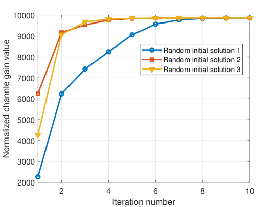
Figure 2: Convergence behaviour of Algorithm 1 with different initial solutions.

Fig. 2 illustrates the convergence of Algorithm 1 using different initial solutions. In this figure, the normalized channel gain value means the channel gain divided by the noise power, i.e., $\frac{\left|{\bm{g}}_{1}+{\bm{U}}_{1}^{H}{\bm{v}}\right|^{2}}{\sigma^{2}}$. It can be seen that the proposed algorithm converges fast, and eight iterations are sufficient to converge, which shows the effectiveness of the proposed algorithm.

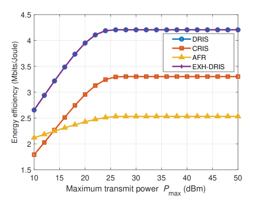
Figure 3: Energy efficiency versus the maximum transmit power $P_{\max}$ of the BS.

Fig. 3 shows how the energy efficiency changes as the maximum transmit power of the BS varies. In this figure, the EXH-DRIS scheme is an exhaustive search method that can find a near optimal solution of problem (9). Hereinafter, the EXH-DRIS scheme refers to the proposed DRIS algorithm with 1000 initial starting points. In this simulation, EXH-DRIS can obtain 1000 solutions, and the solution with the highest energy efficiency is treated as the near optimal solution. It is shown that the energy efficiency of all schemes first increases and then remains stable as the maximum transmit power of the BS increases. This is because energy efficiency is not a monotonically increasing function of the maximum transmit power, as shown in (17). When $P_{\max}\geq 25$ dBm, the exceed transmit power is not used since it will decrease the energy efficiency. Fig. 3 also shows that the proposed DRIS scheme outperforms the CRIS and AFR schemes. For high maximum transmit power of the BS, DRIS can increase up to 27% and 68% energy efficiency compared to CRIS and AFR, respectively. Moreover, the proposed DRIS scheme achieves almost the same performance as the EXH-DRIS scheme, which indicates that the proposed DRIS can achieve the near optimum solution.

Figure 4: Sum-rate versus the maximum transmit power $P_{\max}$ of the BS with $R=0$.

Fig. 4 shows how the sum-rate changes as the maximum transmit power of the BS varies. It is found that the sum-rate of all schemes linearly increases with the logarithmic maximum transmit power of the BS. We can see that AFR achieves the best performance. This is because the AF relay is an active terminal by transmitting the received signal to the user, while the RIS is only a passive reflecting structure. From Fig. 4, DRIS can increase up to 26% sum-rate compared to CRIS. This is due to the benefits of distributed deployment. Multiple RISs are spatially distributed in DRIS, which can provide more than one path of received signal compared to CRIS with only one central RIS.

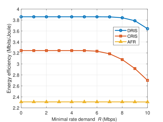
Figure 5: Energy efficiency versus the minimum rate demand $R$.

Fig. 5 shows the energy efficiency versus the minimum rate demand. From this figure, DRIS achieves the best performance. In particular, DRIS can achieve up to 33% and 67% gains in terms of energy efficiency compared to CRIS and AFR, respectively. Both DRIS and CRIS always achieve a better performance than AFR. This is due to the fact that the power consumption for the RIS is much lower compared to the transmit power of the AF relay. It is also found that DRIS achieves better performance than CRIS, which indicates the benefit of distributed deployment of RISs. This is because DRIS exhibits a better spectrum efficiency compared to CRIS, and CRIS is more sensitive to high minimum rate demand than DRIS. From Fig. 5, we can observe that the energy efficiency remains stable when minimum rate demand is low. However, for a high minimum rate demand, the energy efficiency decreases rapidly for both CRIS and DRIS. This is because a high minimum rate demand requires the BS to transmit with high power, which consequently degrades the energy efficiency performance. Fig. 5 also demonstrates that, as the minimum rate demand increases, the energy efficiency of CRIS decreases faster than DRIS.

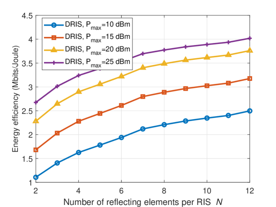
Figure 6: Energy efficiency versus the number of reflecting elements $N$ for each RIS with $L=4$.

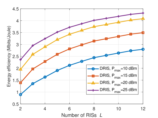
Figure 7: Energy efficiency versus the number of RISs $L$ with $N=4$.

Figs. 6 and 7 show the energy efficiency versus the number of reflecting elements for each RIS and the number of RISs, respectively. From these figures, we can see that the energy efficiency of DRIS monotonically increases with the number of reflecting elements and the number of RISs. This is because large number of reflecting elements and RISs can lead to high spectral efficiency and the power consumption of introducing additional reflecting elements and RISs is low, which result in high energy efficiency of the system. According to Figs. 6 and 7, it is also found that the energy efficiency of DRIS increases faster with the number of RISs than that with the number of reflecting elements for each RIS, which shows that it is more energy efficient to deploy with multiple RISs. For the same total number of all reflecting elements, i.e., the same $NL$, we consider the following two configurations: (a) $N=12$, $L=4$, $P_{\max}=25$ dBm, and (b) $N=4$, $L=12$, $P_{\max}=25$ dBm. From Figs. 6 and 7, the energy efficiency of configuration (a) is 4.0 Mbits/Joule and the energy efficiency of configuration (b) is 4.3 Mbits/Joule, which shows that the energy efficiency of $L>N$ is better than that of $L<N$.

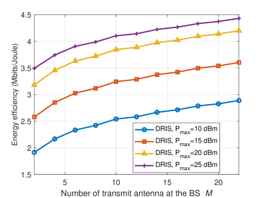
Figure 8: Energy efficiency versus the number of transmit antennas $M$ at the BS.

In Fig. 8, we show the energy efficiency versus the number of transmit antennas at the BS with various maximum transmit power of the BS. Fig. 8 demonstrates that the energy efficiency increases rapidly for a small number of transmit antennas at the BS, however, this increase becomes slower for a larger number of transmit antennas at the BS. This is because a high number of transmit antennas at the BS leads to high power consumption, which consequently decreases the slope of increase of the energy efficiency. From Fig. 8, we can also see that the energy efficiency increases with the maximum transmit power of the BS for a given number of transmit antenna at the BS. Moreover, for high value of the BS maximum transmit power, the energy efficiency slowly increases with the maximum transmit power.

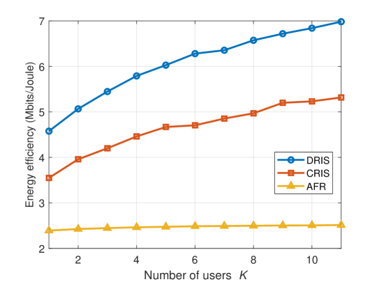
Figure 9: Energy efficiency versus the number of users.

The energy efficiency versus the number of users is shown in Fig. 9. From Fig. 9, we observe that the energy efficiency of AFR is always low due to the fact that the transmit power of the AF relay is high. Clearly, the proposed DRIS is always better than CRIS and AFR especially when the number of users is large.

VI Conclusion

In this paper, we have investigated the resource allocation problem for a wireless communication network with distributed RISs. The RIS phase shifts, BS transmit beamforming, and RIS on-off status were jointly optimized to maximize the system energy efficiency while satisfying minimum rate demand, maximum transmit power, and unit-modulus constraints. To solve this problem, we have proposed two iterative algorithms with low complexity for the single-user case and multi-user case, respectively. In particular, the phase optimization problem was solved by using the SCA method, where the closed-form solution was obtained at each step for the single-user case. Numerical results have shown that the proposed scheme outperforms conventional schemes in terms of energy efficiency, especially for small maximum transmit power and large number of users.

References

• [1] W. Saad, M. Bennis, and M. Chen, “A vision of 6G wireless systems: Applications, trends, technologies, and open research problems,” IEEE Network, 2020 (To appear).
• [2] M. Chen, Z. Yang, W. Saad, C. Yin, H. V. Poor, and S. Cui, “A joint learning and communications framework for federated learning over wireless networks,” arXiv preprint arXiv:1909.07972, 2019.
• [3] H. Q. Ngo, E. G. Larsson, and T. L. Marzetta, “Energy and spectral efficiency of very large multiuser MIMO systems,” IEEE Trans. Commun., vol. 61, no. 4, pp. 1436–1449, Apr. 2013.
• [4] G. Y. Li, Z. Xu, C. Xiong, C. Yang, S. Zhang, Y. Chen, and S. Xu, “Energy-efficient wireless communications: Tutorial, survey, and open issues,” IEEE Wireless Commun., vol. 18, no. 6, pp. 28–35, Dec. 2011.
• [5] S. Buzzi, I. Chih-Lin, T. E. Klein, H. V. Poor, C. Yang, and A. Zappone, “A survey of energy-efficient techniques for 5G networks and challenges ahead,” IEEE J. Sel. Areas Commun., vol. 34, no. 4, pp. 697–709, Apr. 2016.
• [6] S. Zhang, S. Xu, G. Y. Li, and E. Ayanoglu, “First 20 years of green radios,” arXiv preprint arXiv:1908.07696, 2019.
• [7] W. Xu, Y. Cui, H. Zhang, G. Y. Li, and X. You, “Robust beamforming with partial channel state information for energy efficient networks,” IEEE J. Sel. Areas Commun., vol. 33, no. 12, pp. 2920–2935, Dec. 2015.
• [8] E. Basar, M. Di Renzo, J. de Rosny, M. Debbah, M.-S. Alouini, and R. Zhang, “Wireless communications through reconfigurable intelligent surfaces,” arXiv preprint arXiv:1906.09490, 2019.
• [9] S. Zhang and R. Zhang, “Capacity characterization for intelligent reflecting surface aided MIMO communication,” arXiv preprint arXiv:1910.01573, 2019.
• [10] S. Hu, K. Chitti, F. Rusek, and O. Edfors, “User assignment with distributed large intelligent surface (LIS) systems,” in Proc. IEEE Int. Symposium Personal, Indoor Mobile Radio Commun., Bologna, Italy, Sep. 2018, pp. 1–6.
• [11] C. Pan, H. Ren, K. Wang, W. Xu, M. Elkashlan, A. Nallanathan, and L. Hanzo, “Intelligent reflecting surface for multicell MIMO communications,” arXiv preprint arXiv:1907.10864, 2019.
• [12] Q.-U.-A. Nadeem, A. Kammoun, A. Chaaban, M. Debbah, and M.-S. Alouini, “Large intelligent surface assisted MIMO communications,” arXiv preprint arXiv:1903.08127, 2019.
• [13] Z. Yang, J. Shi, Z. Li, M. Chen, W. Xu, and M. Shikh-Bahaei, “Energy efficient rate splitting multiple access (RSMA) with reconfigurable intelligent surface,” in Proc. IEEE Int. Conf. Commun. Workshop, 2020 (To appear), pp. 1–6.
• [14] S. V. Hum and J. Perruisseau-Carrier, “Reconfigurable reflectarrays and array lenses for dynamic antenna beam control: A review,” IEEE Trans. Antennas Prop., vol. 62, no. 1, pp. 183–198, Jan. 2013.
• [15] J. Huang, Q. Li, Q. Zhang, G. Zhang, and J. Qin, “Relay beamforming for amplify-and-forward multi-antenna relay networks with energy harvesting constraint,” IEEE Signal Process. Lett., vol. 21, no. 4, pp. 454–458, Apr. 2014.
• [16] K. Ntontin, M. Di Renzo, J. Song, F. Lazarakis, J. de Rosny, D.-T. Phan-Huy, O. Simeone, R. Zhang, M. Debbah, G. Lerosey, M. Fink, S. Tretyakov, and S. Shamai, “Reconfigurable intelligent surfaces vs. relaying: Differences, similarities, and performance comparison,” arXiv preprint arXiv:1908.08747, 2019.
• [17] C. Huang, S. Hu, G. C. Alexandropoulos, A. Zappone, C. Yuen, R. Zhang, M. Di Renzo, and M. Debbah, “Holographic MIMO surfaces for 6G wireless networks: Opportunities, challenges, and trends,” arXiv preprint arXiv:1911.12296, 2019.
• [18] C. Huang, A. Zappone, M. Debbah, and C. Yuen, “Achievable rate maximization by passive intelligent mirrors,” in Proc. IEEE Int. Conf. Acoust., Speech and Signal Process., Calgary, Canada, April 2018, pp. 3714–3718.
• [19] M. Jung, W. Saad, Y. Jang, G. Kong, and S. Choi, “Performance analysis of large intelligence surfaces (LISs): Asymptotic data rate and channel hardening effects,” IEEE Trans. Wireless Commun., 2020 (To appear).
• [20] M. Jung, W. Saad, M. Debbah, and C. S. Hong, “On the optimality of reconfigurable intelligent surfaces (RISs): Passive beamforming, modulation, and resource allocation,” arXiv preprint arXiv:1910.00968, 2019.
• [21] C. Pan, H. Ren, K. Wang, M. Elkashlan, A. Nallanathan, J. Wang, and L. Hanzo, “Intelligent reflecting surface enhanced MIMO broadcasting for simultaneous wireless information and power transfer,” arXiv preprint arXiv:1908.04863, 2019.
• [22] M.-M. Zhao, Q. Wu, M.-J. Zhao, and R. Zhang, “Intelligent reflecting surface enhanced wireless network: Two-timescale beamforming optimization,” arXiv preprint arXiv:1912.01818, 2019.
• [23] H. Shen, W. Xu, S. Gong, Z. He, and C. Zhao, “Secrecy rate maximization for intelligent reflecting surface assisted multi-antenna communications,” IEEE Commun. Lett., vol. 23, no. 9, pp. 1488–1492, Sep. 2019.
• [24] X. Yu, D. Xu, Y. Sun, D. W. K. Ng, and R. Schober, “Robust and secure wireless communications via intelligent reflecting surfaces,” arXiv preprint arXiv:1912.01497, 2019.
• [25] C. Huang, A. Zappone, G. C. Alexandropoulos, M. Debbah, and C. Yuen, “Reconfigurable intelligent surfaces for energy efficiency in wireless communication,” IEEE Trans. Wireless Commun., vol. 18, no. 8, pp. 4157–4170, Aug. 2019.
• [26] L. N. Ribeiro, S. Schwarz, M. Rupp, and A. L. de Almeida, “Energy efficiency of mmwave massive MIMO precoding with low-resolution DACs,” IEEE J. Sel. Topics Signal Process., vol. 12, no. 2, pp. 298–312, May 2018.
• [27] R. Méndez-Rial, C. Rusu, N. González-Prelcic, A. Alkhateeb, and R. W. Heath, “Hybrid MIMO architectures for millimeter wave communications: Phase shifters or switches?” IEEE Access, vol. 4, pp. 247–267, Jan. 2016.
• [28] D. Tse and P. Viswanath, Fundamentals of Wireless Communication.   Cambridge University Press, 2005.
• [29] Q. Wu and R. Zhang, “Intelligent reflecting surface enhanced wireless network via joint active and passive beamforming,” IEEE Trans. Wireless Commun., vol. 18, no. 11, pp. 5394–5409, Nov. 2019.
• [30] Q. Wu and R. Zhang, “Beamforming optimization for wireless network aided by intelligent reflecting surface with discrete phase shifts,” CoRR, vol. abs/1906.03165, 2019. [Online]. Available: http://arxiv.org/abs/1906.03165
• [31] A. Zappone, E. Bjornson, L. Sanguinetti, and E. Jorswieck, “Globally optimal energy-efficient power control and receiver design in wireless networks,” IEEE Trans Signal Process., vol. 65, no. 11, pp. 2844–2859, June 2017.
• [32] W. Dinkelbach, “On nonlinear fractional programming,” Management Science, vol. 13, no. 7, pp. 492–498, 1967.
• [33] S. Boyd and L. Vandenberghe, Convex Optimization.   Cambridge University Press, 2004.
• [34] D. P. Bertsekas, Convex Optimization Theory.   Athena Scientific Belmont, 2009.
• [35] Y. Pan, M. Chen, Z. Yang, N. Huang, and M. Shikh-Bahaei, “Energy-efficient NOMA-based mobile edge computing offloading,” IEEE Communications Letters, vol. 23, no. 2, pp. 310–313, 2019.
• [36] M. Chen, Z. Yang, W. Saad, C. Yin, H. V. Poor, and S. Cui, “Performance optimization of federated learning over wireless networks,” in 2019 IEEE Global Communications Conference (GLOBECOM), 2019, pp. 1–6.
• [37] Z. Yang, M. Chen, W. Saad, C. S. Hong, and M. Shikh-Bahaei, “Energy efficient federated learning over wireless communication networks,” arXiv preprint arXiv:1911.02417, 2019.
• [38] M. Grant, S. Boyd, and Y. Ye, “CVX: Matlab software for disciplined convex programming,” 2008.
• [39] M. S. Lobo, L. Vandenberghe, S. Boyd, and H. Lebret, “Applications of second-order cone programming,” Linear algebra and its applications, vol. 284, no. 1-3, pp. 193–228, 1998.
• [40] F. Zarringhalam, B. Seyfe, M. Shikh-Bahaei, G. Charbit, and H. Aghvami, “Jointly optimized rate and outer loop power control with single- and multi-user detection,” IEEE Transactions on Wireless Communications, vol. 8, no. 1, pp. 186–195, 2009.
• [41] A. Zappone, P. Cao, and E. A. Jorswieck, “Energy efficiency optimization in relay-assisted MIMO systems with perfect and statistical CSI,” IEEE Trans. Signal Process., vol. 62, no. 2, pp. 443–457, Jan. 2014.