Prediction of Dst during solar minimum using in situ measurements at L5
Abstract
Geomagnetic storms resulting from high-speed streams can have significant negative impacts on modern infrastructure due to complex interactions between the solar wind and geomagnetic field. One measure of the extent of this effect is the Kyoto index. We present a method to predict from data measured at the Lagrange 5 (L5) point, which allows for forecasts of solar wind development 4.5 days in advance of the stream reaching the Earth. Using the STEREO-B satellite as a proxy, we map data measured near L5 to the near-Earth environment and make a prediction of the from this point using the Temerin-Li model enhanced from the original using a machine learning approach. We evaluate the method accuracy with both traditional point-to-point error measures and an event-based validation approach. The results show that predictions using L5 data outperform a 27-day solar wind persistence model in all validation measures but do not achieve a level similar to an L1 monitor. Offsets in timing and the rapidly-changing development of in comparison to and reduce the accuracy. Predictions of from L5 have an RMSE of nT, which is double the error of nT using measurements conducted near the Earth. The most useful application of L5 measurements is shown to be in predicting the minimum for the next four days. This method is being implemented in a real-time forecast setting using STEREO-A as an L5 proxy, and has implications for the usefulness of future L5 missions.
Space Weather
Space Research Institute, Austrian Academy of Sciences, Graz, Austria Heliophysics Science Division, NASA Goddard Space Flight Center, Greenbelt, MD 20771, USA Institute of Physics, University of Graz, Graz, Austria Conrad Observatory, Zentralanstalt für Meteorologie und Geodynamik, Vienna, Austria
Rachel Baileyrachel.bailey@oeaw.ac.at
In-situ L5 data can be used for Dst forecasts at Earth and perform better than 27-day recurrence
Low consistency of Bz over multiple days limits the accuracy of Dst predicted from L5
This method performs best when forecasting the minimum Dst during SIRs
1 Introduction
The solar wind has myriad effects on the Earth’s magnetic field, among them the enhancement of the ring current around the Earth’s equator [Gonzalez \BOthers. (\APACyear1994)]. Through streams of charged particles, the solar wind injects energy into the ring current and thereby reduces the global magnetic field strength [Daglis \BOthers. (\APACyear1999)]. This can have consequences on GPS and satellite communication as well as flight operations where crew may be exposed to greater levels of radiation [Schrijver \BOthers. (\APACyear2015)]. The extent of the enhancement and resultant reduction in field strength is often given by the disturbance storm time index, . This is an hourly value derived from geomagnetic field variations measured at four observatories (Honolulu, Kakioka, San Juan and Hermanus) below in geomagnetic latitude [Mayaud (\APACyear1980)]. Different levels of geomagnetic activity are often described by the minimum of reached, with a nT denoting an extreme geomagnetic storm, nT being an intense storm, and nT being only a moderate storm. A nT is sometimes used to denote weak geomagnetic storms. The largest negative values of are seen almost exclusively in storms caused by interplanetary coronal mass ejections/ICMEs [Borovsky \BBA Denton (\APACyear2006)], while moderate storms occur throughout the solar cycle [Richardson \BOthers. (\APACyear2001), Tsurutani \BOthers. (\APACyear2006)]. These more common, milder storms are driven by high-speed streams and stream interaction regions/SIRs [Alves \BOthers. (\APACyear2006), Jian \BOthers. (\APACyear2006)], and \citeARichardson2000 showed that high-speed streams lead to 70% of geomagnetic activity during solar minimum. In rare cases SIR-driven storms can also become major geomagnetic events [Richardson \BOthers. (\APACyear2006)] with an expected maximum possible storm strength of nT.
Although the official Kyoto is derived solely from ground-based field measurements, a very good estimate of the upcoming can be made based on in situ solar wind data from satellites at the Lagrange 1 (L1) point [<]e.g. most recently the DSCOVR satellite, see¿Burt2012. This allows for a prediction lead time of 10–50 minutes, with the amount of time determined by solar wind speed between L1 and Earth. The state-of-the-art approach in this respect is the model of \citeATemerin2006, an empirical technique that achieves a Pearson correlation coefficient between the observed and predicted values of for the seven years of data evaluated. This model depends solely on solar wind input, and the variation in at one point depends on both the solar wind at that point in time and past modelled timesteps.
For forecasts beyond a half-hour window, we look now to possible future missions to the L5 point, which sits behind the Earth in its orbit and roughly 4.5 days in advance for corotating solar wind structures. A space weather mission at this point to perform in situ solar wind measurements has been discussed many times before [Gopalswamy \BOthers. (\APACyear2011), Lavraud \BOthers. (\APACyear2016), Hapgood (\APACyear2017)], and presents a strong opportunity for accurate forecasts of space weather events with a much enhanced lead time ranging from hours to days. As shown in \citeAThomas2018, a solar wind monitor at the L5 point can provide very good forecasts of the ambient solar wind variations, of which high-speed streams and SIRs are of primary interest.
In this work we show how predictions of the index at Earth can be made using L5 data and discuss the applicability and accuracy of the method. This is carried out using data from the Solar Terrestrial Relations Observatory Behind [<]STEREO-B, NASA, see¿Kaiser2005 satellite, which crossed the L5 point in late 2009, as a proxy for a future L5 mission. Data from this satellite is mapped to L1 as if it had been measured there by correcting for both time passed in solar rotation speed and solar wind expansion [Thomas \BOthers. (\APACyear2018)], and a method for predicting the from L1 data is then applied. The accuracy of the forecast is evaluated using a combination of traditional error metrics (e.g. correlation coefficient, mean error) as well as a method considering the prediction of events (e.g. minimum) without comparing the development point-to-point. Past studies have looked at predicting the general solar wind properties [Simunac \BOthers. (\APACyear2009), Turner \BBA Li (\APACyear2011), Kohutova \BOthers. (\APACyear2016), Temmer \BOthers. (\APACyear2018), Owens \BOthers. (\APACyear2019)] while this study aims specifically to determine how well the development of and geomagnetic effects can be predicted using L5 data. The results also include a brief analysis of the sensitivity of prediction to offsets in measurements of the magnetic field. This study serves as a verification for methods that are now being implemented in real-time using STEREO-A data as it crosses the L5 point and moves towards the Earth.
2 Methods
2.1 Mapping L5 data to L1
Studies using the STEREO satellites (launched in 2006) as proxies for satellites positioned at L5 have been undertaken in the past. \citeASimunac2009 mapped data from L5 to L1 using a time shift determined by the synodic rotation period of the Sun and showed good agreement between the solar wind speed and density measured at the two locations. \citeATurner2011 evaluated the correlation between time-shifted measurements ahead in the Parker spiral and L1 data. It was shown that while the correlation in solar wind speed remains high, there is rarely much correlation in magnetic field components. \citeAThomas2018 continued in this thread but went a step further and carried out a comprehensive analysis of solar wind forecasting skill using data measured near L5.
To map data measured at L5 or thereabouts to L1, we use the same approach as described in \citeAThomas2018 and apply a time shift to the data measured at STEREO-B assuming a rotation in the solar wind equivalent to the rotation speed at the solar equator of roughly 27 days (). Here we use a synodic rotation period of days as given in \citeAOwens2013. A second adjustment to the time to correct for differences in radial distances () and solar wind expansion timing is calculated as follows based on Eq. 1 from \citeASimunac2009:
| (1) |
where and are the radial distances of L1 and STEREO-B from the Sun, while is the mean solar wind speed at the time of measurement. is the difference in longitude between the Earth/L1 and STEREO-B. is the variable for solar rotation speed . The total time shift , which varies with longitudinal distance between the satellite and Earth, is then added to the time of measurements from STEREO-B. Since this results in a new range of times with increasing difference between the new and original values as STEREO-B moves away, the measurements are interpolated back to periodic hourly time values.
A second adjustment is applied to the solar wind data to account for areal expansion of the solar wind at different radii and in the Parker spiral [Kivelson \BBA Russell (\APACyear1995)]. All variables are multiplied by a correction factor determined by the ratio between the distance of STEREO-B and L1 . The rate of expansion for the density is assumed to behave according to the inverse-square law [Kumar \BBA Rust (\APACyear1996)], while the magnetic fielc components scale according to factors as given in \citeAHanneson2020 varying between -2 and -1. In the case of STEREO-B, which was at a distance greater than AU, this means that the solar wind was corrected backwards and effectively compressed to L1.
2.2 Prediction of from L1
There are many different models for predicting the index from solar wind measurements. Earlier models from \citeABurton1975 and \citeAObrien2000 achieve a reasonable level of accuracy. When using the OMNI2 data set as input and comparing the results to the true Kyoto values, they have correlation coefficients of and respectively. One of the most exhaustive L1-to- algorithms is undoubtedly the semi-empirical model developed first in \citeATemerin2002 for the years 1995–1999, which was later extended to the year 2002 in \citeATemerin2006. This model has a linear correlation of around for in the periods the model was intended for (in good agreement with the original work), although when using it for predictions beyond this period (2002–2019), there is a linear drift away from the real of about nT/year due to the inclusion of a time-dependent variable in the model [Temerin \BBA Li (\APACyear2015)]. After applying a simple linear correction for the drift, the correlation for this model in future times is still very good at 0.90 on average. Due to the dependence of the model on local time, the input for data mapped to L1 was the time it was expected to arrive there and not the time it was measured.
The \citeATemerin2006 method (henceforth called TL2006) makes very good predictions of at the Earth using either data measured at L1 or data mapped to L1 using the aforementioned time-shifting method. A small improvement can be made to the model through application of a machine learning algorithm from the Python package SciKit-Learn to provide a correction factor for the base drift-corrected TL2006 output. The algorithm is a gradient boosting regressor (GBR), which develops an ensemble of basic regressors to calculate output (correction to ) based on the provided input. The input was the same set of variables provided to the TL2006 method (solar wind speed, density, and magnetic field components along with time). Some feature engineering was applied to the input variables to provide more information to the GBR such as including a solar wind pressure term and time derivative of to evaluate which variables improved the prediction, and those that did not lead to an improvement were removed. The most important addition was the introduction a “ring-current term” (with both current and past values from the prior 24 hours) based on the method in \citeAObrien2000. The ring-current term described most of the variation not accounted for by the TL2006 method, and the prediction of from solar wind measurements using the TL2006 method plus this GBR correction value (enhanced method or ETL2006) leads to an improved average linear correlation of 0.95 and reduced RMSE between real and predicted over the time range 2000–2018. In this study we apply the model using the enhancement throughout.
3 Data
The NASA OMNI2 data set was used for getting the measurements of the solar wind in the near-Earth environment and the values for the Kyoto (the real values to which all predictive models are compared). The machine learning algorithm providing the correction to the TL2006 prediction method was trained on the Kyoto data set for 2000-2018.
STEREO-B one-minute resolution PLASTIC [Galvin \BOthers. (\APACyear2008)] and IMPACT [Luhmann \BOthers. (\APACyear2008)] instrument data was used as a proxy for data measured at L5. STEREO-B differs from a true L5 mission in two ways: firstly, it was constantly in motion and moving further away from the Earth in its orbit; and secondly, it was also at a greater distance from the Sun than the Earth ( AU). These differences were both accounted for using the approach defined in the methods section. Beacon data, which is low-resolution data sent soon (minutes) after measurement, was used rather than the higher-quality science data that arrives later to simulate the forecasting application of this model in a real-time operation scenario. This will have an effect on the final results, although we would not expect the quality to be greatly degraded by using beacon rather than science data. The data was also downsampled via interpolation to one-hour resolution.
STEREO-B data is given in the reference frame STBHGRTN , a spacecraft-centric reference frame with pointing from the Sun to the spacecraft with the Sun as the origin, as the cross-product of the rotational axis with the -component, and as the normal to these two pointing out of the ecliptic. While the satellite is still in the geospace environment, the STBHGRTN coordinate system can be transformed to GSE by flipping the and directions. For calculation purposes, this is converted to GSM according to the algorithms given in \citeAHapgood1992. The STBHGRTN frame rotates with the spacecraft as it moves away from the Earth but we assume a rotation of the solar wind with the mapping of data measured at STEREO-B to L1, and therefore can perform the same coordinate transformation to quasi-GSE (as if the measurements had been made in the geospace environment) and then to GSM. All spacecraft positions in this work are given in heliocentric Earth equatorial (HEEQ) longitudes and latitudes, in which the -axis is parallel to the Sun’s rotation axis and the -axis is the intersection of the solar equator and solar central meridian as seen from Earth.
Because STEREO-B is always moving and only spent a short amount of time around the actual L5 point at , for the purposes of this study we consider the location of L5 to be in longitude in addition to evaluating overall statistics for the range to . Comparisons of results in the next sections will refer to the two data sets as the full data set and the reduced data set. The time range in the full data set covers five years from Feb 2007 until Jan 2012. The time range for the reduced range of angles from STEREO-B near L5 is almost six months from August 2009 until February 2010, which encapsulates almost the entire solar minimum, meaning this is the optimal time range to evaluate L5-based ambient solar wind prediction.
To allow comparison to a simple reference baseline model, a third data set was created as a persistence model, as this has been shown to achieve reasonable accuracy with a solar wind recurrence rate of 27.27 days [Owens \BOthers. (\APACyear2013)]. For this, the same OMNI2 data was taken after being shifted into the future by 27.27 days. These models are referred to as OMNI, STB and PERS in short form and plots throughout the text. In order to calculate reliably, any gaps in the data were linearly interpolated over.
ICMEs that occured at one location or in one data set and not the other were removed from the data using start and end times given in the HELCATS ICMECAT catalogue [Möstl \BOthers. (\APACyear2017)], which covered the period of evaluation for both STEREO-B and measurements near the Earth (in this case with the WIND satellite). This was carried out for all comparison data sets after STEREO-B had been time-shifted with ICME start and end times being corrected to the new shifted times. In total, three sets of ICMEs were removed from all data sets: those at STEREO-B, those at L1, and those at L1 shifted by 27.27 days for the persistence model. This reduces the size of the total data set by 12%.
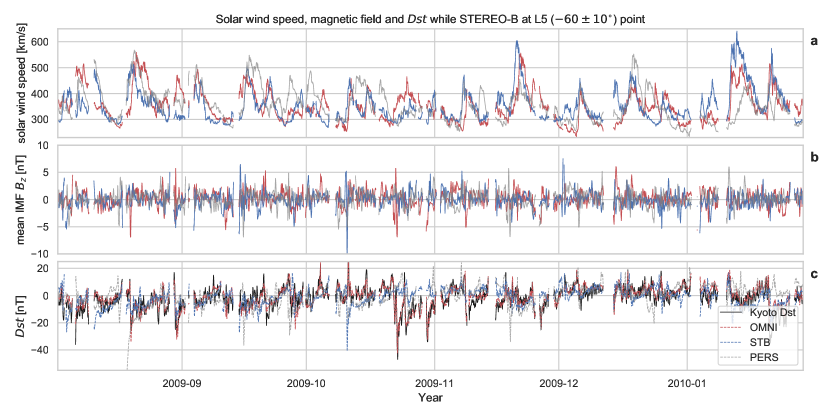
An example of solar wind speed, vertical magnetic field and values from the three data sets is plotted in Fig. 1, in which the time range covered by STEREO-B when it was near the L5 point () is shown. The STEREO-B data has already been time-shifted according to the solar rotation speed to Earth, and is plotted against the OMNI data for comparison. The high-speed streams observed at STEREO-B are easy to identify and generally overlap with those in the OMNI data, although in some cases they arrive earlier or later than their counterparts at Earth. Gaps in the data are ICMEs that have been removed. As can be seen in the comparison of , the red line with predicted from the OMNI data very closely matches the actual Kyoto , while in the mapped STEREO-B prediction there are still large variations. The persistence model (grey) performs worse than the STEREO-B approach.
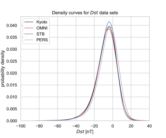
The distribution of values in (both observed and predicted) according to the different models is plotted in Fig. 2. The OMNI, Kyoto and PERS data sets have very similar distributions, but the STB values have a slightly higher peak close to zero and fewer values in the positive region.
See Sec. 6 for a list of all data sources.
4 Results
The goodness of prediction of values predicted from data measured near the L5 point will be evaluated in this section. First, the goodness will be measured according to standard error metrics, and then the models will be compared using an event-based approach looking additionally at the forecasting of events within 24-hour windows.
4.1 Accuracy of prediction
We first evaluate the accuracy of a prediction using data from the L5 point using standard metrics such as the Pearson correlation coefficient (PCC), mean absolute error (MAE), mean error (ME) and root-mean-square error (RMSE) of the predicted values subtracted from the observed. The results for each data set are listed in Table 1.
Predictions from the OMNI data set consistently achieve a very good level of accuracy compared to the real Kyoto , which is to be expected given the good behaviour of the ETL2006 model in general, although predictions using STEREO-B data are considerably worse. When comparing the STEREO-B/L5 predictions to the persistence model, we see that the prediction using STEREO-B data is better in all measures. Errors in both these models are usually twice as large as those from the OMNI model.
| Mean | Min. | ME | MAE | RMSE | PCC | ||
|---|---|---|---|---|---|---|---|
| OMNI | -7.49 | -140.38 | -0.24 | 3.89 | 5.04 | 0.90 | |
| STB | -7.28 | -172.16 | -0.21 | 8.40 | 12.25 | 0.41 | |
| PERS | -5.38 | -164.96 | -2.11 | 9.40 | 13.42 | 0.33 | |
| OMNI | -1.13 | -42.34 | -0.89 | 3.38 | 4.38 | 0.85 | |
| STB | -1.45 | -40.67 | -0.56 | 6.63 | 8.89 | 0.25 | |
| PERS | -0.83 | -62.81 | -1.19 | 8.04 | 10.90 | 0.12 |

In Fig. 3, the PCC and RMSE are both plotted as a function of longitudinal difference between Earth and STEREO-B. Each point was calculated for the data measured at the point of longitude , which led to time ranges of two to seven months being evaluated because STEREO-B was not moving away from Earth at a constant rate with regards to longitudinal distance. As can be seen in the figure, predictions of using OMNI data fairly consistently achieve a PCC of and an RMSE of roughly nT, while the accuracy of the STEREO-B prediction degrades with increasing distance from the Earth, as would be expected. Note some features of the plot at first glance seem peculiar but can be easily explained. The sudden rise in PCC beyond the of -100 is a result of exceptionally quiet periods with only small values of . The peak in RMSE just before of -100 is a result of one particularly geo-effective high-speed stream ( nT) being observed at both STEREO-B and L1 but with an offset of multiple days.
In Fig. 3a, the curves in the figure show fits to the PCC values as a decaying function of , and we see that at a of , the predictions from STEREO-B data seem to have dropped to roughly the same accuracy as the persistence model. The PCC here starts at close to the Earth and drops to 0 at around .
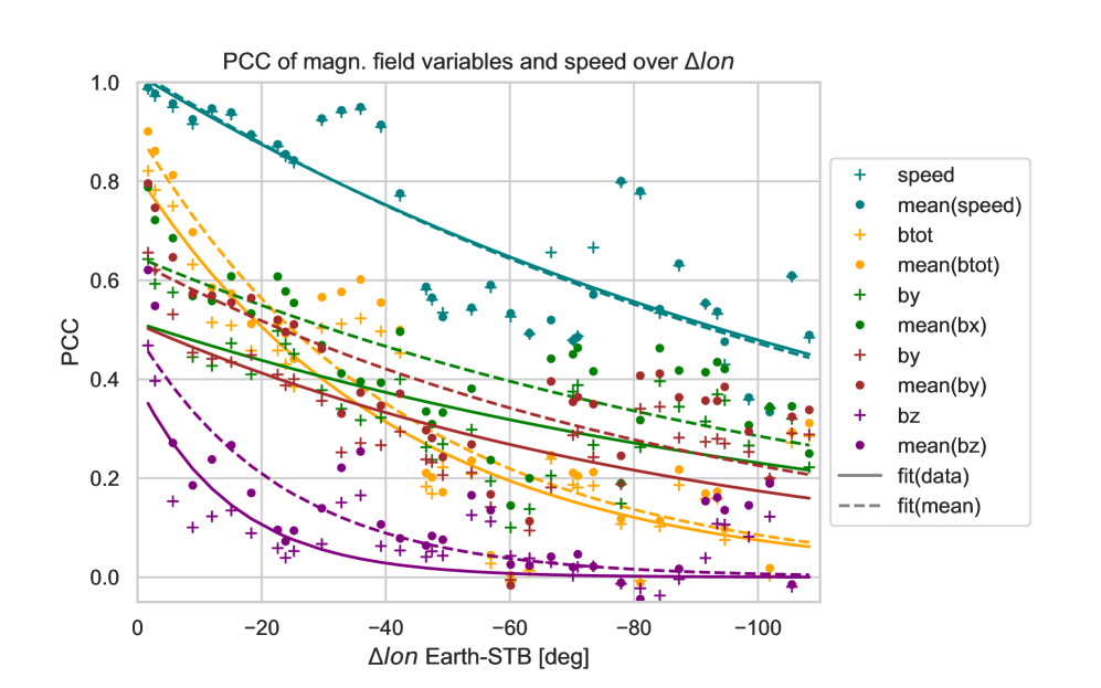
Fig. 4 explains this quick drop-off showing the correlations between solar wind variables in OMNI and STEREO-B with increasing , both as hourly values and the means over a window of 4 hours. The solar wind speed remains highly correlated, which is to be expected due to the rotation of coronal holes and the relatively slow temporal development of high-speed streams. The correlation for total magnetic field and the - and -components also remains good throughout, but the -component drops off quickly and the correlation has already nearly reached 0 at . Due to the strong dependence of on [<]see e.g.¿Gonzalez1987, it is not surprising that we also lose accuracy in prediction fairly quickly. What is however useful to note from Fig. 4 is that the correlation in mean() and the other components remains good beyond the point at which the correlation of hourly values has dropped significantly.
In Fig. 3, the results from the persistence model are also included in grey, and we see that there is a similar downward slope and decreasing correlation over time even though we would expect this to stay constant. This suggests that, for this time period at least, there may have been other effects in the solar wind leading to a reduction in accuracy from the prediction due to more rapid changes in the solar wind structures and high-speed streams. This is likely explained by the increase in solar activity as the Sun entered the rising phase of the solar cycle in 2011/2012. We would observe greater numbers of short-duration coronal holes closer to solar maximum in addition to the more regular coronal holes and high-speed streams that dominate the variations otherwise. Although time does not increase linearly from point to point in Fig. 3, on the whole it spans five years and we can look at the general development of PCC and RMSE over time. Both show a gradual decrease in accuracy as solar activity increases, which is most important to note for the persistence model that serves as a benchmark for the others. When taking this into account, a prediction using STEREO-B data at greater values of may also be a reasonable approach that is simply not represented well here due to the more active period evaluated.
At the L5 point, the PCC for the STEREO-B model is around . Unfortunately, looking at the points alone we see that the approach performed particularly badly at precisely this angle, although from the overall statistics we can deduce that this was only a short-duration dissonance that had little to do with the spacecraft position itself. This may instead be a result of latitudinal difference between the two satellites, which we look at in the following.
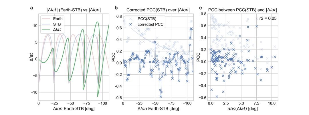
The dynamics of the outflowing solar wind in the heliospheric current sheet have a strong latitudinal dependence, with differences of a few degrees resulting in large variations in the shape and timing of the arriving solar wind structures. In \citeASimunac2009 and \citeAThomas2018, for example, differences in latitude between two spacecraft were shown to have a notable effect on forecasting skill. To quantify this effect in this study, we look at the accuracy metrics with the longitudinal dependence removed plotted against the absolute difference in latitude between the two measuring points, STEREO-B and Earth. See Fig. 5 for a depiction of this approach. This was achieved by subtracting the slope of the longitudinal dependence for STEREO-B (centre plot, light blue line) along with the slope in the OMNI values to account for unrelated changes over time. Interestingly, few of the metrics show any correlation with a difference in latitude, with the exception being the MAE and RMSE, which correlate mildly with with a PCC of (increasing accuracy with increasing , a confusing result). All other metrics have correlations , such as the PCC showed as an example in the figure (centre and right). If the range of is reduced to to (in which the most periodic rotational behaviour was observed), a more predictable set of behaviour emerges. The correlation values for PCC, RMSE and MAE with are -0.21, 0.24 and 0.15 respectively, suggesting small dependencies on leading to a decrease in accuracy. Since an analysis of the whole range did not show the same pattern, we can deduce that discrepancies caused by the increase in solar activity later in the cycle far outweigh the effects of latitudinal difference in regards to accuracy.
As a sanity check, the same metrics with and without ICMEs were also compared, and the results were as expected. Predictions of using OMNI data were equally good with and without ICMEs, but there was a small improvement in the metrics for data predicted using the STEREO-B data and the persistence model because the transient events unrelated to their measurements had been removed. An analysis of errors with the input solar wind data split into high-speed streams and slow solar wind was also carried out, with the results showing that the errors in calculated for fast solar wind (above a threshold 1.25 times the median speed or km/s) are slightly ( %) larger than those for slow solar wind. In a further test, we also looked at the same evaluation without scaling of the magnetic field components to correct for different orbital distances to see if this step was necessary. Not scaling the solar wind input led to a very small increase in the errors (e.g. an RMSE of nT increasing to nT), showing that the scaling of magnetic field to correct for a distance of 0.1 AU (at maximum) does have an effect on the accuracy on the forecast, although it is minimal.
4.2 Event-based analysis
An interesting alternative to standard point-to-point measures that quantitatively assess the magnitude of the forecast error at each time step is to consider each time step as an event/non-event. The primary advantages of an event-based validation analysis are as follows. Firstly, periods of weak, moderate and enhanced geomagnetic activity are weighted equally by simple point-to-point comparison measures. However, end-users of operational real-time space weather models are usually more interested in accurately predicting times of enhanced values, while the exact evolution in time of the is in most cases of secondary importance. Secondly, outliers in the predicted times can have a significant influence on the error measures and correlation coefficients determined. In context, an efficient approach is to label each time step in the predicted and observed timeline as an event/non-event [Owens (\APACyear2018)]. An example of this approach applied to high-speed streams can be found in \citeAReiss2016, in which the OSEA software used for this analysis was also used.
In this study, we define an “event” as any time step the exceeded (or went below) a certain threshold. In this case we defined nT as the threshold for a weak geomagnetic storm. The value of nT, usually the threshold for a moderate storm, was also seen in the period evaluated, but did not occur often enough to allow for a reasonable statistical analysis. Similarly, values beyond nT arose so infrequently that it was not worth considering them here, and we restrict ourselves to looking at all events below a level of nT as a proxy for “mild geomagnetic activity”. Using the corresponding threshold values, we label each time step as an event or non-event in the measured and predicted time series, and for the case of everything below the threshold was an event. By cross-checking the events/non-events between true and predicted , we count the number of hits (true positives; TPs), false alarms (false positives; FPs), misses (false negatives, FNs) and correct rejections (true negatives; TNs) and summarise them in the so-called contingency table. From the entries of the contingency table, we can compute different skill measures, including the True Positive Rate TPR = TP/(TP + FN) and the False Positive Rate FPR = FP/(FP + TN). While the TPR is the proportion of correctly predicted events among all the events, the FPR is the proportion of non-events wrongly predicted as events.
Moreover, we compute the Threat Score TS = TP/(TP+FP+FN) as a measure of the model performance, Bias B = (TP+FP)/(TP+FN) indicating whether the number of observations is underforecast () or overforecast (), and the True Skill Statistics TSS = TPR - FPR as a measure of the overall model performance. The TSS is defined in the range [-1,1] where a perfect prediction would be equal to 1 (or -1, for a perfect inverse prediction), and a TSS equal to 0 indicates no predictive ability of the forecast model. It is important to note that the TSS is unbiased by the proportion of predicted and observed events [Hanssen \BBA Kuipers (\APACyear1965), Bloomfield \BOthers. (\APACyear2012)]. Since the number of non-events exceeds the number of events by 10 to 1, the TSS is very well suited for the validation analysis conducted in this study. For a more thorough discussion of the skill measures applied here, we would like to refer the interested reader to \citeAJolliffe2003.
| TP | FP | FN | TN | TSS | Bias | AUC | |||
|---|---|---|---|---|---|---|---|---|---|
| OMNI | 843 | 618 | 280 | 225 | 36622 | 0.73 | 1.07 | 0.94 | |
| STB | 843 | 127 | 729 | 716 | 36173 | 0.13 | 1.02 | 0.74 | |
| PERS | 843 | 75 | 581 | 768 | 36321 | 0.05 | 0.78 | 0.70 | |
| OMNI | 6 | 4 | 0 | 2 | 3701 | 0.67 | 0.67 | 0.92 | |
| STB | 6 | 0 | 1 | 6 | 3700 | 0.00 | 0.17 | 0.63 | |
| PERS | 6 | 0 | 17 | 6 | 3684 | 0.00 | 2.83 | 0.59 | |
| OMNI | 218 | 177 | 40 | 41 | 2886 | 0.80 | 1.00 | - | |
| STB | 218 | 65 | 131 | 153 | 2795 | 0.25 | 0.90 | - | |
| PERS | 218 | 43 | 117 | 175 | 2809 | 0.16 | 0.73 | - |
Table 2 shows the contingency table entries and the skill measures computed over the full and reduced time ranges. We find that the prediction using OMNI/L1 data has a very high level of accuracy in all measures, and in comparison the prediction from STEREO-B/L5 is only somewhat better than a persistence model. Both STB and PERS models show a tendency to underforecast when considering the full data set.
Interestingly, we see that for the time STEREO-B was around L5 (in the reduced data set), it managed to forecast 0 of the events below the threshold, while the persistence model also forecast 0 but achieved an impressive number of FPs. It is hard to carry out statistics for this period because it was an extremely quiet time, with only 6 events below the nT threshold over six months. To look at a less time-sensitive approach, we consider an additional forecasting method.
The bottom rows of Table 2 show the event-based analysis for the prediction of the minimum in the next hours (with a -hour resolution), and in this way we consider the predictions while ignoring possible errors in timing of hours. (For the OMNI model, with a maximum forecast time of 30–60 minutes, this is obviously a pointless measure, but it is left in for comparison.) Here it becomes clear that the L5 monitor outperforms the persistence model while also achieving a higher TSS score than when simply applied to all data. In this case, the ratio of FPs to TPs is also greatly reduced from around 6 to 2.
A straightforward approach to illustrate the trade-off between the proportion of correctly predicted events (TPR) and the proportion of erroneously predicted events (FPR) for different event thresholds is the so-called receiver operator characteristic (ROC) curve. ROC curves are a helpful diagnostic to compare and quantitatively assess the predictive skill of forecast models. They illustrate how the number of correctly classified events varies with the number of incorrectly classified non-events for each model investigated here. In other words, they show the trade-off between the completeness of events and the contamination with non-events. To illustrate the predictive abilities of the different forecast models in a single summary variable, we also compute the area under the curve (AUC) defined between 0 and 1, where the best results are equal to 1.
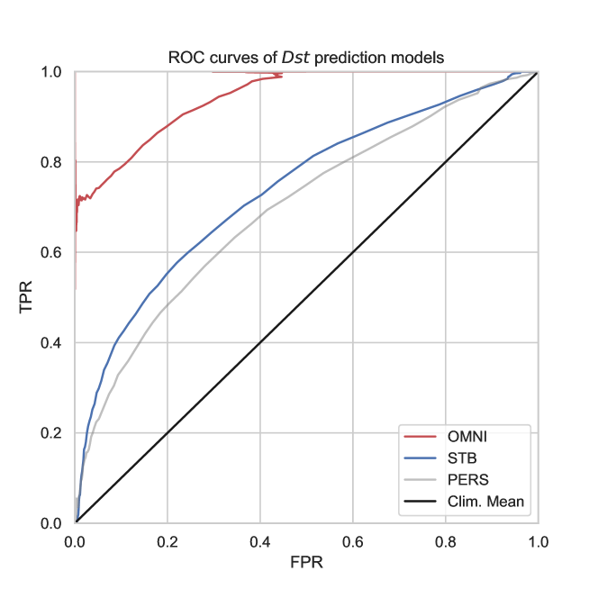
Fig. 6 shows the ROC curves for all models using the full data sets. At a glance it is clear that the OMNI model far outperforms the models using STEREO-B and PERS data, and the STEREO-B model is almost always somewhat better than persistence.
4.3 Sensitivity of model to field measurements
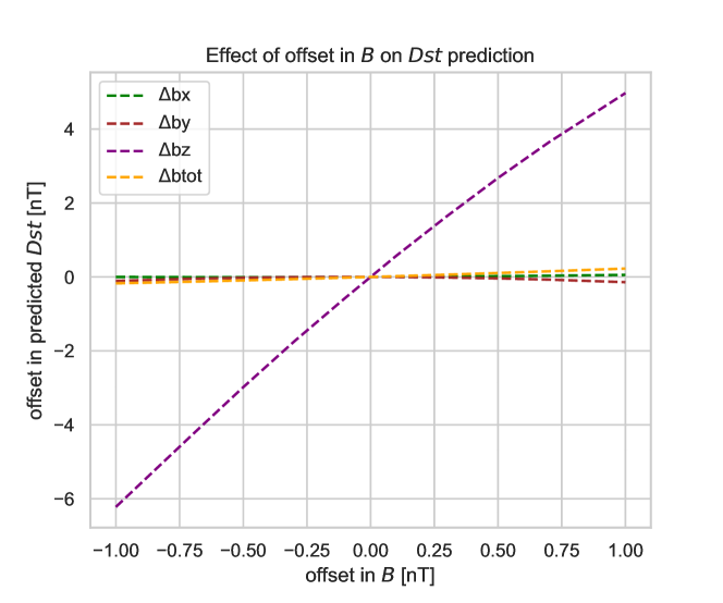
Here we also include a brief evaluation of the sensitivity of the ETL2006 prediction model to magnetic field measurements and the effect of possible offsets in the measurements. To achieve this, the ETL2006 model was used to predict from two years of OMNI data to simply assess model sensitivity independent of any other factors. Fig. 7 shows the dependence of predicted on offsets in magnetic field measurements. An error of nT in the component leads to an error of nT in the predicted , although offsets in all other components have almost no effect. This is useful to know for future L1 and L5 missions, which rely on in-flight calibration methods such as that described in \citeAPlaschke2019, to have an estimate of the error in the prediction if the error in the magnetic field measurements are known.
5 Discussion and conclusions
In order to evaluate the possibility of forecasting the index from the L5 point with a lead time of a few days, we have looked at in situ solar wind data measured by STEREO-B as it crossed the L5 point. This was mapped to L1 in time and space according to the solar rotation speed and expansion of the solar wind and high speed streams. The mapped data is used to make a prediction of and the results were then compared to the Kyoto as well as predicted from an L1 monitor and a 27-day persistence model. This method is useful for predicting geomagnetic effects from high-speed streams and SIRs, but can not provide forecasts for transient events such as ICMEs. The results can be summarised as follows:
-
•
A prediction of the index from data measured at L5 does not achieve a level of accuracy similar to predictions made using L1 data, but it performs better than a 27-day solar wind persistence model in all standard measures. Geomagnetic effects in particular are hard to predict due to the rapidly-changing development of .
-
•
The error in the prediction can be quantified using the MAE, which at the L5 point in the STB model has an average value of 8 nT, which is double the error from L1 at 4 nT. Offsets in measurements of nT can cause an offset error in the predicted of nT.
-
•
As the values of magnetic field variations correlate much more strongly when looking at mean values, a method of predicting the from means taken over multiple hours would likely be a strong forecasting method, and this should be considered for operational purposes.
-
•
The usefulness of L5 data in predicting minima in the next 24 hours is reasonable and performs better than a persistence model.
-
•
A strong dependence of the accuracy of the predicted on latitudinal difference between the L5 proxy and L1 measurements could not be determined.
Unsurprisingly, because is so badly predicted from L5 due to the rapid changes in magnetic field [<]as discussed in detail in¿Thomas2018, it is difficult to quantify the geo-effectiveness of a high-speed stream in advance using data from somewhere as far-removed as L5 because of the strong dependence on in causing geomagnetic effects [Gonzalez \BBA Tsurutani (\APACyear1987)]. This was compounded by the fact that the coherence of high-speed streams when STEREO-B was closest to the L5 point was uncharacteristically low, and so most of the results have been based on general trends in forecasting capabilities across a much wider range of longitudes from the Earth from 0 to , at which point the error appeared to match that seen in the persistence model. As described in \citeAVerbanac2011, also has a strong correlation with the solar wind speed, which shows that is not the only input to the model providing valuable information on how the develops. A further effect that may lead to reduced accuracy is stream-stream or stream-CME interaction. In some cases, a CME bracketed in an SIR can give rise to enhanced geo-effectiveness in the stream [Chen \BOthers. (\APACyear2019)]. This would be particularly effective if such a case were to occur at L5, drastically changing the nature of the predicted high-speed stream that would later arrive at Earth. Regardless, we have shown that predictions of from data at L5 certainly outperform a persistence model, especially when looking at predictions of minimum in the next 24 hours or days.
This work was carried out to validate application of the methods in an operational setting, and as such STEREO beacon data, which arrived in near real-time, was used. Beacon data is, however, of considerably lower quality than the science data, which arrives much later. Due to developments in on-board processing since the STEREO launch in 2006, real-time data to be expected from upcoming space weather satellites should be of better quality than the original beacon data and may be closer in quality to the science data. For comparison, the same parameters as discussed above were evaluated for STEREO Level 2 scientific data, and an increase in accuracy was observed. This was on a small scale (a correlation of instead of , for example), but shows that the data from newer satellites with more advanced real-time data transfer should achieve a slightly higher accuracy for predictions than presented here.
At the moment, STEREO-A is slowly approaching the Earth in its orbit, meaning that it can function as a proxy for real-time L5 forecasts for both the solar wind variables and . This study has functioned as a verification for a real-time model currently running using STEREO-A data, which at the time of writing is at a longitude of . For this forecast, we can assume an error in predicted of nT from the average MAE at the L5 point reached by STEREO-B. The knowledge gathered throughout this real-time forecasting using STEREO-A will be invaluable in preparation for setting up effective predictive methods relying on a real future L5 space weather mission.
6 Sources of Data and Supplementary Material
Solar wind in situ data:
OMNI2: https://spdf.gsfc.nasa.gov/pub/data/omni/low_res_omni/
STEREO-B (BEACON): https://stereo-ssc.nascom.nasa.gov/data/beacon/behind/
STEREO-B (L2): https://stereo-ssc.nascom.nasa.gov/data/ins_data/impact/level2/behind/magplasma/
Catalogues:
ICMECAT: https://doi.org/10.6084/m9.figshare.4588315.v1
Software:
Jupyter Notebook for this work: https://doi.org/10.6084/m9.figshare.11733909
Predstorm (Python, data handling): https://doi.org/10.5281/zenodo.3750749
OSEA (Matlab, statistical analysis): https://doi.org/10.5281/zenodo.3753104
HelioSat (Python, data download): https://doi.org/10.5281/zenodo.3749561
Acknowledgements.
The Python packages for data download and handling that this work is based on (Predstorm v0.1, HelioSat v0.3.1) are open-source and under development and are available on our group GitHub page (https://github.com/helioforecast). The statistical analysis was carried out using Matlab solar wind analysis scripts OSEA. Furthermore, the exact script that was used to create the results and plots shown here (in Jupyter Notebook format) is available. See Section 6 for the links to the data and scripts, and instructions for installation in the repositories. R.L.B, C.M., M.A.R., A.J.W., U.V.A., T.A. and J.H. thank the Austrian Science Fund (FWF): P31659-N27, J4160-N27, P31521-N27, P31265-N27. We would like to thank the editor and reviewers for their helpful responses, which led to improvement of this manuscript.References
- Alves \BOthers. (\APACyear2006) \APACinsertmetastarAlves2006{APACrefauthors}Alves, M\BPBIV., Echer, E.\BCBL \BBA Gonzalez, W\BPBID. \APACrefYearMonthDay2006. \BBOQ\APACrefatitleGeoeffectiveness of corotating interaction regions as measured by Dst index Geoeffectiveness of corotating interaction regions as measured by dst index.\BBCQ \APACjournalVolNumPagesJournal of Geophysical Research: Space Physics111A7. \PrintBackRefs\CurrentBib
- Bloomfield \BOthers. (\APACyear2012) \APACinsertmetastarBloomfield2012{APACrefauthors}Bloomfield, D\BPBIS., Higgins, P\BPBIA., McAteer, R\BPBIT\BPBIJ.\BCBL \BBA Gallagher, P\BPBIT. \APACrefYearMonthDay2012Mar. \BBOQ\APACrefatitleToward Reliable Benchmarking of Solar Flare Forecasting Methods Toward reliable benchmarking of solar flare forecasting methods.\BBCQ \APACjournalVolNumPagesThe Astrophysical Journal Letters7472L41. \PrintBackRefs\CurrentBib
- Borovsky \BBA Denton (\APACyear2006) \APACinsertmetastarBorovsky2006{APACrefauthors}Borovsky, J\BPBIE.\BCBT \BBA Denton, M\BPBIH. \APACrefYearMonthDay2006. \BBOQ\APACrefatitleDifferences between CME-driven storms and CIR-driven storms Differences between CME-driven storms and CIR-driven storms.\BBCQ \APACjournalVolNumPagesJournal of Geophysical Research: Space Physics111A7. \PrintBackRefs\CurrentBib
- Burt \BBA Smith (\APACyear2012) \APACinsertmetastarBurt2012{APACrefauthors}Burt, J.\BCBT \BBA Smith, B. \APACrefYearMonthDay2012March. \BBOQ\APACrefatitleDeep Space Climate Observatory: The DSCOVR mission Deep space climate observatory: The dscovr mission.\BBCQ \BIn \APACrefbtitle2012 IEEE Aerospace Conference 2012 ieee aerospace conference (\BPG 1-13). \PrintBackRefs\CurrentBib
- Burton \BOthers. (\APACyear1975) \APACinsertmetastarBurton1975{APACrefauthors}Burton, R\BPBIK., McPherron, R\BPBIL.\BCBL \BBA Russell, C\BPBIT. \APACrefYearMonthDay1975. \BBOQ\APACrefatitleAn empirical relationship between interplanetary conditions and Dst An empirical relationship between interplanetary conditions and dst.\BBCQ \APACjournalVolNumPagesJournal of Geophysical Research (1896-1977)80314204-4214. \PrintBackRefs\CurrentBib
- Chen \BOthers. (\APACyear2019) \APACinsertmetastarChen2019{APACrefauthors}Chen, C., Liu, Y\BPBID., Wang, R., Zhao, X., Hu, H.\BCBL \BBA Zhu, B. \APACrefYearMonthDay2019oct. \BBOQ\APACrefatitleCharacteristics of a Gradual Filament Eruption and Subsequent CME Propagation in Relation to a Strong Geomagnetic Storm Characteristics of a gradual filament eruption and subsequent CME propagation in relation to a strong geomagnetic storm.\BBCQ \APACjournalVolNumPagesThe Astrophysical Journal884190. \PrintBackRefs\CurrentBib
- Daglis \BOthers. (\APACyear1999) \APACinsertmetastarDaglis1999{APACrefauthors}Daglis, I\BPBIA., Thorne, R\BPBIM., Baumjohann, W.\BCBL \BBA Orsini, S. \APACrefYearMonthDay1999. \BBOQ\APACrefatitleThe terrestrial ring current: Origin, formation, and decay The terrestrial ring current: Origin, formation, and decay.\BBCQ \APACjournalVolNumPagesReviews of Geophysics374407-438. \PrintBackRefs\CurrentBib
- Galvin \BOthers. (\APACyear2008) \APACinsertmetastarGalvin2008{APACrefauthors}Galvin, A\BPBIB., Kistler, L\BPBIM., Popecki, M\BPBIA., Farrugia, C\BPBIJ., Simunac, K\BPBID\BPBIC., Ellis, L.\BDBLSteinfeld, D. \APACrefYearMonthDay2008. \BBOQ\APACrefatitleThe Plasma and Suprathermal Ion Composition (PLASTIC) Investigation on the STEREO Observatories The plasma and suprathermal ion composition (plastic) investigation on the stereo observatories.\BBCQ \BIn C\BPBIT. Russell (\BED), (\BPGS 437–486). \APACaddressPublisherNew York, NYSpringer New York. \PrintBackRefs\CurrentBib
- Gonzalez \BOthers. (\APACyear1994) \APACinsertmetastarGonzalez1994{APACrefauthors}Gonzalez, W\BPBID., Joselyn, J\BPBIA., Kamide, Y., Kroehl, H\BPBIW., Rostoker, G., Tsurutani, B\BPBIT.\BCBL \BBA Vasyliunas, V\BPBIM. \APACrefYearMonthDay1994. \BBOQ\APACrefatitleWhat is a geomagnetic storm? What is a geomagnetic storm?\BBCQ \APACjournalVolNumPagesJournal of Geophysical Research: Space Physics99A45771-5792. \PrintBackRefs\CurrentBib
- Gonzalez \BBA Tsurutani (\APACyear1987) \APACinsertmetastarGonzalez1987{APACrefauthors}Gonzalez, W\BPBID.\BCBT \BBA Tsurutani, B\BPBIT. \APACrefYearMonthDay1987. \BBOQ\APACrefatitleCriteria of interplanetary parameters causing intense magnetic storms (Dst -100 nT) Criteria of interplanetary parameters causing intense magnetic storms (Dst -100 nT).\BBCQ \APACjournalVolNumPagesPlanetary and Space Science3591101 - 1109. \PrintBackRefs\CurrentBib
- Gopalswamy \BOthers. (\APACyear2011) \APACinsertmetastarGopalswamy2011{APACrefauthors}Gopalswamy, N., Davila, J., Cyr, O\BPBIS., Sittler, E., Auchère, F., Duvall, T.\BDBLCollier, M. \APACrefYearMonthDay2011. \BBOQ\APACrefatitleEarth-Affecting Solar Causes Observatory (EASCO): A potential International Living with a Star Mission from Sun–Earth L5 Earth-affecting solar causes observatory (easco): A potential international living with a star mission from sun–earth l5.\BBCQ \APACjournalVolNumPagesJournal of Atmospheric and Solar-Terrestrial Physics735658 - 663. \PrintBackRefs\CurrentBib
- Hanneson \BOthers. (\APACyear2020) \APACinsertmetastarHanneson2020{APACrefauthors}Hanneson, C., Johnson, C\BPBIL., Mittelholz, A., Al Asad, M\BPBIM.\BCBL \BBA Goldblatt, C. \APACrefYearMonthDay2020. \BBOQ\APACrefatitleDependence of the Interplanetary Magnetic Field on Heliocentric Distance at 0.3–1.7 AU: A Six-Spacecraft Study Dependence of the interplanetary magnetic field on heliocentric distance at 0.3–1.7 au: A six-spacecraft study.\BBCQ \APACjournalVolNumPagesJournal of Geophysical Research: Space Physics1253e2019JA027139. \PrintBackRefs\CurrentBib
- Hanssen \BBA Kuipers (\APACyear1965) \APACinsertmetastarHanssen1965{APACrefauthors}Hanssen, A.\BCBT \BBA Kuipers, W. \APACrefYear1965. \APACrefbtitleOn the Relationship Between the Frequency of Rain and Various Meteorological Parameters: (with Reference to the Problem Of Objective Forecasting) On the relationship between the frequency of rain and various meteorological parameters: (with reference to the problem of objective forecasting). \APACaddressPublisherStaatsdrukerij. {APACrefURL} https://books.google.at/books?id=nTZ8OgAACAAJ \PrintBackRefs\CurrentBib
- Hapgood (\APACyear1992) \APACinsertmetastarHapgood1992{APACrefauthors}Hapgood, M. \APACrefYearMonthDay1992. \BBOQ\APACrefatitleSpace physics coordinate transformations: A user guide Space physics coordinate transformations: A user guide.\BBCQ \APACjournalVolNumPagesPlanetary and Space Science405711 - 717. \PrintBackRefs\CurrentBib
- Hapgood (\APACyear2017) \APACinsertmetastarHapgood2017{APACrefauthors}Hapgood, M. \APACrefYearMonthDay2017. \BBOQ\APACrefatitleL1L5Together: Report of Workshop on Future Missions to Monitor Space Weather on the Sun and in the Solar Wind Using Both the L1 and L5 Lagrange Points as Valuable Viewpoints L1l5together: Report of workshop on future missions to monitor space weather on the sun and in the solar wind using both the l1 and l5 lagrange points as valuable viewpoints.\BBCQ \APACjournalVolNumPagesSpace Weather155654-657. \PrintBackRefs\CurrentBib
- Jian \BOthers. (\APACyear2006) \APACinsertmetastarJian2006{APACrefauthors}Jian, L., Russell, C., Luhmann, J.\BCBL \BBA Skoug, R. \APACrefYearMonthDay2006. \BBOQ\APACrefatitleProperties of stream interactions at one AU during 1995–2004 Properties of stream interactions at one AU during 1995–2004.\BBCQ \APACjournalVolNumPagesSolar Physics2391-2337–392. \PrintBackRefs\CurrentBib
- Jolliffe \BBA Stephenson (\APACyear2003) \APACinsertmetastarJolliffe2003{APACrefauthors}Jolliffe, I.\BCBT \BBA Stephenson, D. \APACrefYear2003. \APACrefbtitleForecast Verification: A Practitioner’s Guide in Atmospheric Science Forecast verification: A practitioner’s guide in atmospheric science. \APACaddressPublisherWiley. {APACrefURL} https://books.google.com/books?id=Qm2MjWVvUywC \PrintBackRefs\CurrentBib
- Kaiser (\APACyear2005) \APACinsertmetastarKaiser2005{APACrefauthors}Kaiser, M. \APACrefYearMonthDay2005. \BBOQ\APACrefatitleThe STEREO mission: an overview The stereo mission: an overview.\BBCQ \APACjournalVolNumPagesAdvances in Space Research3681483 - 1488. \PrintBackRefs\CurrentBib
- Kivelson \BBA Russell (\APACyear1995) \APACinsertmetastarIntroSpacePhysics{APACrefauthors}Kivelson, M.\BCBT \BBA Russell, C. \APACrefYear1995. \APACrefbtitleIntroduction to Space Physics Introduction to space physics. \APACaddressPublisherCambridge University Press. \PrintBackRefs\CurrentBib
- Kohutova \BOthers. (\APACyear2016) \APACinsertmetastarKohutova2016{APACrefauthors}Kohutova, P., Bocquet, F\BHBIX., Henley, E\BPBIM.\BCBL \BBA Owens, M\BPBIJ. \APACrefYearMonthDay2016. \BBOQ\APACrefatitleImproving solar wind persistence forecasts: Removing transient space weather events, and using observations away from the Sun-Earth line Improving solar wind persistence forecasts: Removing transient space weather events, and using observations away from the sun-earth line.\BBCQ \APACjournalVolNumPagesSpace Weather1410802-818. \PrintBackRefs\CurrentBib
- Kumar \BBA Rust (\APACyear1996) \APACinsertmetastarKumar1996{APACrefauthors}Kumar, A.\BCBT \BBA Rust, D\BPBIM. \APACrefYearMonthDay1996. \BBOQ\APACrefatitleInterplanetary magnetic clouds, helicity conservation, and current-core flux-ropes Interplanetary magnetic clouds, helicity conservation, and current-core flux-ropes.\BBCQ \APACjournalVolNumPagesJournal of Geophysical Research: Space Physics101A715667-15684. \PrintBackRefs\CurrentBib
- Lavraud \BOthers. (\APACyear2016) \APACinsertmetastarLavraud2016{APACrefauthors}Lavraud, B., Liu, Y., Segura, K., He, J., Qin, G., Temmer, M.\BDBLFernández, J. \APACrefYearMonthDay2016. \BBOQ\APACrefatitleA small mission concept to the Sun–Earth Lagrangian L5 point for innovative solar, heliospheric and space weather science A small mission concept to the sun–earth lagrangian l5 point for innovative solar, heliospheric and space weather science.\BBCQ \APACjournalVolNumPagesJournal of Atmospheric and Solar-Terrestrial Physics146171 - 185. \PrintBackRefs\CurrentBib
- Luhmann \BOthers. (\APACyear2008) \APACinsertmetastarLuhmann2008{APACrefauthors}Luhmann, J\BPBIG., Curtis, D\BPBIW., Schroeder, P., McCauley, J., Lin, R\BPBIP., Larson, D\BPBIE.\BDBLGosling, J\BPBIT. \APACrefYearMonthDay2008. \BBOQ\APACrefatitleSTEREO IMPACT Investigation Goals, Measurements, and Data Products Overview Stereo impact investigation goals, measurements, and data products overview.\BBCQ \BIn C\BPBIT. Russell (\BED), (\BPGS 117–184). \APACaddressPublisherNew York, NYSpringer New York. \PrintBackRefs\CurrentBib
- Mayaud (\APACyear1980) \APACinsertmetastarMayaud1980{APACrefauthors}Mayaud, P\BPBIN. \APACrefYearMonthDay1980. \BBOQ\APACrefatitleDerivation, Meaning, and Use of Geomagnetic Indices Derivation, Meaning, and Use of Geomagnetic Indices.\BBCQ \APACjournalVolNumPagesWashington DC American Geophysical Union Geophysical Monograph Series22. \PrintBackRefs\CurrentBib
- Möstl \BOthers. (\APACyear2017) \APACinsertmetastarMoestl2017{APACrefauthors}Möstl, C., Isavnin, A., Boakes, P\BPBID., Kilpua, E\BPBIK\BPBIJ., Davies, J\BPBIA., Harrison, R\BPBIA.\BDBLZhang, T\BPBIL. \APACrefYearMonthDay2017. \BBOQ\APACrefatitleModeling observations of solar coronal mass ejections with heliospheric imagers verified with the Heliophysics System Observatory Modeling observations of solar coronal mass ejections with heliospheric imagers verified with the heliophysics system observatory.\BBCQ \APACjournalVolNumPagesSpace Weather157955-970. \PrintBackRefs\CurrentBib
- O’Brien \BBA McPherron (\APACyear2000) \APACinsertmetastarObrien2000{APACrefauthors}O’Brien, T\BPBIP.\BCBT \BBA McPherron, R\BPBIL. \APACrefYearMonthDay2000. \BBOQ\APACrefatitleAn empirical phase space analysis of ring current dynamics: Solar wind control of injection and decay An empirical phase space analysis of ring current dynamics: Solar wind control of injection and decay.\BBCQ \APACjournalVolNumPagesJournal of Geophysical Research: Space Physics105A47707-7719. \PrintBackRefs\CurrentBib
- Owens (\APACyear2018) \APACinsertmetastarOwens2018{APACrefauthors}Owens, M\BPBIJ. \APACrefYearMonthDay2018\APACmonth11. \BBOQ\APACrefatitleTime-Window Approaches to Space-Weather Forecast Metrics: A Solar Wind Case Study Time-Window Approaches to Space-Weather Forecast Metrics: A Solar Wind Case Study.\BBCQ \APACjournalVolNumPagesSpace Weather161847-1861. {APACrefDOI} 10.1029/2018SW002059 \PrintBackRefs\CurrentBib
- Owens \BOthers. (\APACyear2013) \APACinsertmetastarOwens2013{APACrefauthors}Owens, M\BPBIJ., Challen, R., Methven, J., Henley, E.\BCBL \BBA Jackson, D\BPBIR. \APACrefYearMonthDay2013. \BBOQ\APACrefatitleA 27 day persistence model of near-Earth solar wind conditions: A long lead-time forecast and a benchmark for dynamical models A 27 day persistence model of near-earth solar wind conditions: A long lead-time forecast and a benchmark for dynamical models.\BBCQ \APACjournalVolNumPagesSpace Weather115225-236. \PrintBackRefs\CurrentBib
- Owens \BOthers. (\APACyear2019) \APACinsertmetastarOwens2019{APACrefauthors}Owens, M\BPBIJ., Riley, P., Lang, M.\BCBL \BBA Lockwood, M. \APACrefYearMonthDay2019. \BBOQ\APACrefatitleNear-Earth Solar Wind Forecasting Using Corotation From L5: The Error Introduced By Heliographic Latitude Offset Near-earth solar wind forecasting using corotation from l5: The error introduced by heliographic latitude offset.\BBCQ \APACjournalVolNumPagesSpace Weather1771105-1113. \PrintBackRefs\CurrentBib
- Plaschke (\APACyear2019) \APACinsertmetastarPlaschke2019{APACrefauthors}Plaschke, F. \APACrefYearMonthDay2019. \BBOQ\APACrefatitleHow much solar wind data are sufficient for accurate fluxgate magnetometer offset determinations? How much solar wind data are sufficient for accurate fluxgate magnetometer offset determinations?\BBCQ \APACjournalVolNumPagesGeoscientific Instrumentation, Methods and Data Systems Discussions20191–11. \PrintBackRefs\CurrentBib
- Reiss \BOthers. (\APACyear2016) \APACinsertmetastarReiss2016{APACrefauthors}Reiss, M\BPBIA., Temmer, M., Veronig, A\BPBIM., Nikolic, L., Vennerstrom, S., Schöngassner, F.\BCBL \BBA Hofmeister, S\BPBIJ. \APACrefYearMonthDay2016. \BBOQ\APACrefatitleVerification of high-speed solar wind stream forecasts using operational solar wind models Verification of high-speed solar wind stream forecasts using operational solar wind models.\BBCQ \APACjournalVolNumPagesSpace Weather147495-510. \PrintBackRefs\CurrentBib
- Richardson \BOthers. (\APACyear2000) \APACinsertmetastarRichardson2000{APACrefauthors}Richardson, I\BPBIG., Cliver, E\BPBIW.\BCBL \BBA Cane, H\BPBIV. \APACrefYearMonthDay2000. \BBOQ\APACrefatitleSources of geomagnetic activity over the solar cycle: Relative importance of coronal mass ejections, high-speed streams, and slow solar wind Sources of geomagnetic activity over the solar cycle: Relative importance of coronal mass ejections, high-speed streams, and slow solar wind.\BBCQ \APACjournalVolNumPagesJournal of Geophysical Research: Space Physics105A818203-18213. \PrintBackRefs\CurrentBib
- Richardson \BOthers. (\APACyear2001) \APACinsertmetastarRichardson2001{APACrefauthors}Richardson, I\BPBIG., Cliver, E\BPBIW.\BCBL \BBA Cane, H\BPBIV. \APACrefYearMonthDay2001. \BBOQ\APACrefatitleSources of geomagnetic storms for solar minimum and maximum conditions during 1972–2000 Sources of geomagnetic storms for solar minimum and maximum conditions during 1972–2000.\BBCQ \APACjournalVolNumPagesGeophysical Research Letters28132569-2572. \PrintBackRefs\CurrentBib
- Richardson \BOthers. (\APACyear2006) \APACinsertmetastarRichardson2006{APACrefauthors}Richardson, I\BPBIG., Webb, D\BPBIF., Zhang, J., Berdichevsky, D\BPBIB., Biesecker, D\BPBIA., Kasper, J\BPBIC.\BDBLZhukov, A\BPBIN. \APACrefYearMonthDay2006. \BBOQ\APACrefatitleMajor geomagnetic storms (Dst -100 nT) generated by corotating interaction regions Major geomagnetic storms (dst -100 nt) generated by corotating interaction regions.\BBCQ \APACjournalVolNumPagesJournal of Geophysical Research: Space Physics111A7. \PrintBackRefs\CurrentBib
- Schrijver \BOthers. (\APACyear2015) \APACinsertmetastarSchrijver2015{APACrefauthors}Schrijver, C\BPBIJ., Kauristie, K., Aylward, A\BPBID., Denardini, C\BPBIM., Gibson, S\BPBIE., Glover, A.\BDBLothers \APACrefYearMonthDay2015. \BBOQ\APACrefatitleUnderstanding space weather to shield society: A global road map for 2015–2025 commissioned by COSPAR and ILWS Understanding space weather to shield society: A global road map for 2015–2025 commissioned by COSPAR and ILWS.\BBCQ \APACjournalVolNumPagesAdvances in Space Research55122745–2807. \PrintBackRefs\CurrentBib
- Simunac \BOthers. (\APACyear2009) \APACinsertmetastarSimunac2009{APACrefauthors}Simunac, K\BPBID\BPBIC., Kistler, L\BPBIM., Galvin, A\BPBIB., Popecki, M\BPBIA.\BCBL \BBA Farrugia, C\BPBIJ. \APACrefYearMonthDay2009. \BBOQ\APACrefatitleIn situ observations from STEREO/PLASTIC: a test for L5 space weather monitors In situ observations from STEREO/PLASTIC: a test for L5 space weather monitors.\BBCQ \APACjournalVolNumPagesAnnales Geophysicae27103805–3809. \PrintBackRefs\CurrentBib
- Temerin \BBA Li (\APACyear2002) \APACinsertmetastarTemerin2002{APACrefauthors}Temerin, M.\BCBT \BBA Li, X. \APACrefYearMonthDay2002. \BBOQ\APACrefatitleA new model for the prediction of Dst on the basis of the solar wind A new model for the prediction of dst on the basis of the solar wind.\BBCQ \APACjournalVolNumPagesJournal of Geophysical Research: Space Physics107A12SMP 31-1-SMP 31-8. \PrintBackRefs\CurrentBib
- Temerin \BBA Li (\APACyear2006) \APACinsertmetastarTemerin2006{APACrefauthors}Temerin, M.\BCBT \BBA Li, X. \APACrefYearMonthDay2006. \BBOQ\APACrefatitleDst model for 1995–2002 Dst model for 1995–2002.\BBCQ \APACjournalVolNumPagesJournal of Geophysical Research: Space Physics111A4. \PrintBackRefs\CurrentBib
- Temerin \BBA Li (\APACyear2015) \APACinsertmetastarTemerin2015{APACrefauthors}Temerin, M.\BCBT \BBA Li, X. \APACrefYearMonthDay2015. \BBOQ\APACrefatitleThe Dst index underestimates the solar cycle variation of geomagnetic activity The Dst index underestimates the solar cycle variation of geomagnetic activity.\BBCQ \APACjournalVolNumPagesJournal of Geophysical Research: Space Physics12075603-5607. \PrintBackRefs\CurrentBib
- Temmer \BOthers. (\APACyear2018) \APACinsertmetastarTemmer2018{APACrefauthors}Temmer, M., Hinterreiter, J.\BCBL \BBA Reiss, M\BPBIA. \APACrefYearMonthDay2018. \BBOQ\APACrefatitleCoronal hole evolution from multi-viewpoint data as input for a STEREO solar wind speed persistence model Coronal hole evolution from multi-viewpoint data as input for a STEREO solar wind speed persistence model.\BBCQ \APACjournalVolNumPagesJ. Space Weather Space Clim.8A18. \PrintBackRefs\CurrentBib
- Thomas \BOthers. (\APACyear2018) \APACinsertmetastarThomas2018{APACrefauthors}Thomas, S\BPBIR., Fazakerley, A., Wicks, R\BPBIT.\BCBL \BBA Green, L. \APACrefYearMonthDay2018. \BBOQ\APACrefatitleEvaluating the Skill of Forecasts of the Near-Earth Solar Wind Using a Space Weather Monitor at L5 Evaluating the skill of forecasts of the near-Earth solar wind using a space weather monitor at L5.\BBCQ \APACjournalVolNumPagesSpace Weather167814–828. \PrintBackRefs\CurrentBib
- Tsurutani \BOthers. (\APACyear2006) \APACinsertmetastarTsurutani2006{APACrefauthors}Tsurutani, B\BPBIT., Gonzalez, W\BPBID., Gonzalez, A\BPBIL\BPBIC., Guarnieri, F\BPBIL., Gopalswamy, N., Grande, M.\BDBLVasyliunas, V. \APACrefYearMonthDay2006. \BBOQ\APACrefatitleCorotating solar wind streams and recurrent geomagnetic activity: A review Corotating solar wind streams and recurrent geomagnetic activity: A review.\BBCQ \APACjournalVolNumPagesJournal of Geophysical Research: Space Physics111A7. \PrintBackRefs\CurrentBib
- Turner \BBA Li (\APACyear2011) \APACinsertmetastarTurner2011{APACrefauthors}Turner, D\BPBIL.\BCBT \BBA Li, X. \APACrefYearMonthDay2011\APACmonth01. \BBOQ\APACrefatitleUsing spacecraft measurements ahead of Earth in the Parker spiral to improve terrestrial space weather forecasts Using spacecraft measurements ahead of Earth in the Parker spiral to improve terrestrial space weather forecasts.\BBCQ \APACjournalVolNumPagesSpace Weather9S01002. \PrintBackRefs\CurrentBib
- Verbanac \BOthers. (\APACyear2011) \APACinsertmetastarVerbanac2011{APACrefauthors}Verbanac, G., Vršnak, B., Veronig, A.\BCBL \BBA Temmer, M. \APACrefYearMonthDay2011. \BBOQ\APACrefatitleEquatorial coronal holes, solar wind high-speed streams, and their geoeffectiveness Equatorial coronal holes, solar wind high-speed streams, and their geoeffectiveness.\BBCQ \APACjournalVolNumPagesAstronomy & Astrophysics526A20. \PrintBackRefs\CurrentBib