Ly$\alpha$ Radiative Transfer: Monte-Carlo Simulation of the Wouthuysen-Field Effect

Abstract

A three-dimensional Monte Carlo Ly$\alpha$ radiative transfer (RT) code, named LaRT, is developed to study the Ly$\alpha$ RT and the Wouthuysen-Field (WF) effect. Using the code, we calculate the line profile of Ly$\alpha$ radiation within the multiphase interstellar medium (ISM), with a particular emphasis on gas at low densities. We show that the WF effect is in action: the central portion of the line profile tends to approach a small slice of the Planck function with a color temperature equal to the kinetic temperature of the gas, even in a system with an optical thickness as low as $\tau_{0}\approx 100-500$. We also investigate the effects of the turbulent motion of the ISM on the emergent Ly$\alpha$ spectrum and color temperature. The turbulent motion broadens, as generally expected, the emergent spectrum, but the color temperature is not affected by the turbulent motion in typical astrophysical environments. We utilize two multiphase ISM models, appropriate for the vicinity of the Sun, to calculate the 21-cm spin temperature of neutral hydrogen, including excitation via the Ly$\alpha$ resonant scattering. The first ISM model is a simple clumpy model, while the second is a self-consistent magnetohydrodynamics simulation model using the TIGRESS framework. Ly$\alpha$ photons originating from both H II regions and the collisionally cooling gas are taken into account. We find that the Ly$\alpha$ radiation field is, in general, likely to be strong enough to bring the 21-cm spin temperature of the warm neutral medium close to the kinetic temperature. The escape fraction of Ly$\alpha$ in our ISM models is estimated to be $\approx 7-20\%$.

1. INTRODUCTION

Temperature, density, and ionization degree of the interstellar medium (ISM) are essential parameters to understand heating, cooling, and feedback processes in star and galaxy formation. The 21-cm line originating from the hyperfine energy splitting of the ground state $(n=1)$ of neutral hydrogen is one of the most critical tracers to measure gas temperature and density in the neutral atomic phase of the diffuse ISM, circumgalactic medium (CGM), and intergalactic medium (IGM) (e.g., Schneider et al., 1983; Kulkarni & Heiles, 1987; Schneider, 1989; Swaters et al., 1997; Heiles & Troland, 2003a, b; Murray et al., 2015, 2017). It is often assumed that collisions with electrons, ions, and other H I atoms govern the population of the hyperfine levels of a hydrogen atom. Under a high-density condition in which collisions are frequent, the 21-cm spin temperature (or excitation temperature), which is defined by the relative population of the hyperfine levels, is equal to the gas kinetic temperature. In a low-density medium, however, collisions are not frequent enough to make the spin temperature a good tracer of the gas kinetic temperature; much of the hydrogen would then be “invisible” in observations via the 21-cm line against the cosmic microwave background (CMB) unless other mechanisms establish the spin temperature different from that of the CMB (Bahcall & Ekers, 1969; Deguchi & Watson, 1985).

The Wouthuysen-Field (WF) effect is a radiative mechanism where the resonance scattering (absorption and subsequent re-emission at the same frequency) of Ly$\alpha$ photons indirectly excites the 21-cm line via transitions involving the $n=2$ state of hydrogen as an intermediate state (Wouthuysen, 1952; Field, 1958, 1959b). Wouthuysen (1952) suggested, based on a thermodynamical argument, that the central portion of the Ly$\alpha$ line profile should approach a small slice of the Planck function appropriate to the gas kinetic temperature as neutral hydrogen atoms repeatedly scatter Ly$\alpha$ photons. Field (1959b) explicitly found an asymptotic solution of the time-dependent radiative transfer (RT) equation for isotropic Doppler scattering and showed that the recoil of the scattering hydrogen atoms with a kinetic temperature of $T_{{\rm K}}$ gives rise to a Ly$\alpha$ spectral profile proportional to the exponential function $\exp(-h\nu/k_{{\rm B}}T_{{\rm K}})$ at the line center. The energy exchange between the Ly$\alpha$ photons and the atoms due to recoil causes the exponential slope (color temperature) of the Ly$\alpha$ line profile at the line center to be equal to that of the kinetic temperature. The Planck (or equivalently exponential) function shape at the line center of the Ly$\alpha$ spectrum yields a redistribution over the two hyperfine levels of the ground state of hydrogen.

The indirect pumping effect is found to be indeed important in exciting the 21-cm line in dilute IGM (Field, 1959a). Urbaniak & Wolfe (1981) found that the mean intensity of Ly$\alpha$ is strong enough to govern the spin temperature across an entire H I region that adjoins the H II regions photoionized by Lyman continuum radiation from a quasar. The Ly$\alpha$ recombination followed by ionization via intergalactic UV and X-ray radiation is expected to keep the spin temperature $T_{{\rm s}}$ of the very low-density H I at outer parts of disk galaxies well above the CMB temperature of 2.7 K (Watson & Deguchi, 1984; Corbelli & Salpeter, 1993; Irwin, 1995). Keeney et al. (2005) found that the spin temperature and the kinetic temperature of the halo cloud in a nearby spiral galaxy NGC 3067 probed by the sightline to 3C 232 are approximately equal. They showed that the density of the NGC 3067 clouds is smaller than the density required for particle collisions to thermalize the spin temperature. They thereupon argued that the Ly$\alpha$ photons generated inside the halo cloud drive the spin temperature to the kinetic temperature.

The WF pumping effect is also crucial in understanding the epoch of cosmic reionization. Madau et al. (1997) showed that the non-ionizing UV continuum emitted by early generation stars prior to the epoch of full reionization and then redshifted by the Hubble expansion to the Ly$\alpha$ wavelength in the absorbing IGM rest frame is capable of heating the IGM to a temperature above that of cosmic background radiation (CBR) via the WF coupling. As a consequence, they concluded that most of the neutral IGM would be available for detection at 21 cm in emission. Kuhlen et al. (2006) used numerical hydrodynamic simulations of early structure formation in the Universe and demonstrated that overdense filaments could shine in emission against the CMB, possibly allowing future radio arrays to probe the distribution of neutral hydrogen before cosmic reionization.

In studying the phases of the ISM, the WF effect is also critical. Classical models of heating and cooling in the ISM predict the existence of two neutral phases, the high-density cold neutral medium (CNM) and the low-density warm neutral medium (WNM), which are in thermal and pressure equilibrium (Field et al., 1969; McKee & Ostriker, 1977; Wolfire et al., 1995, 2003). In the CNM, the 21-cm hyperfine transition of hydrogen is thermalized by collisions. On the other hand, in the WNM, collisions with particles cannot thermalize the 21-cm transition. Hence, if only collisions with particles were taken into account, the spin temperature is expected to be much less than the gas kinetic temperature (Field, 1958; Davies & Cummings, 1975; Deguchi & Watson, 1985; Liszt, 2001).

Liszt (2001) investigated how the Ly$\alpha$ scattering would be significant in studying the spin temperature of the WNM using analytic approximations for a uniform slab, derived by Neufeld (1990). The spin temperature was found to be thermalized to the kinetic temperature through the WF coupling when the Ly$\alpha$ radiation field is strong enough in the WNM. He also argued that the density and velocity distribution of the ISM is critical in calculating the Ly$\alpha$ intensity in the WNM. Kim et al. (2014) used three-dimensional (3D) numerical hydrodynamic simulations of the turbulent, multiphase atomic ISM (Kim et al., 2013) to construct synthetic H I 21-cm emission and absorption lines. They considered the WF effect in the synthetic H I 21-cm line observations, adopting a fixed value of the Ly$\alpha$ number density. From a stacking analysis of “residual” 21-cm emission line profiles, Murray et al. (2014) detected a widespread WNM component with excitation temperature $T_{{\rm s}}\sim 7200$ K in the Milky Way, concluding that the Ly$\alpha$ pumping effect is more decisive in the ISM than previously assumed.

Quantifying the requirements for the WF effect is a crucial prerequisite in using the 21-cm line to probe the physical properties of the ISM, CGM, and IGM. Field (1959b) showed that the Ly$\alpha$ spectral profile would have an exponential slope corresponding to the gas kinetic temperature at the limit of an infinite number of scattering. However, surprisingly, very few studies have assessed how a large number of scatterings is required to thermalize the Ly$\alpha$ radiation by recoil. Adams (1971) was the first to quantify how many scatterings are needed for the recoil effect to affect the Ly$\alpha$ RT. He concluded that recoil is negligible unless Ly$\alpha$ undergoes more than $\sim 6\times 10^{10}$ scatterings. Using the large-velocity gradient (LVG) approximation, Deguchi & Watson (1985) found that a Sobolev optical depth of $\sim 10^{6}$, corresponding to a much smaller number of scatterings of $\sim 10^{6}$, is sufficient to bring the color temperature of Ly$\alpha$ to the kinetic temperature of hydrogen gas. Roy et al. (2009) numerically solved the time-dependent RT equation and showed that the color temperature approaches the kinetic temperature after $\sim 10^{4}-10^{5}$ or more scatterings. Recently, Shaw et al. (2017) claimed that the Ly$\alpha$ color temperature would rarely trace the kinetic temperature. These studies were based either on the approximate solution of the RT equation (Field, 1959b; Adams, 1971; Deguchi & Watson, 1985; Roy et al., 2009) or the escape probability method (Shaw et al., 2017).

The Monte-Carlo RT simulation would be the most reliable method to quantify the thermalization condition of the Ly$\alpha$ spectrum due to recoil. Many Monte-Carlo RT codes have been developed to simulate the Ly$\alpha$ RT (Avery & House, 1968; Ahn et al., 2000; Zheng & Miralda-Escudé, 2002a; Cantalupo et al., 2005; Tasitsiomi, 2006; Dijkstra et al., 2006; Verhamme et al., 2006; Semelin et al., 2007; Laursen & Sommer-Larsen, 2007; Laursen et al., 2009; Pierleoni et al., 2009; Forero-Romero et al., 2011; Yajima et al., 2012; Orsi et al., 2012; Gronke & Dijkstra, 2014; Smith et al., 2015). However, they have mostly focused on calculating the Ly$\alpha$ spectrum emergent from astrophysical systems; no RT simulation has been performed to investigate the thermalization condition of Ly$\alpha$ inside the neutral hydrogen medium where Ly$\alpha$ photons propagate.

The above situation motivated the present study. The primary purpose of this work is, therefore, to gain fundamental insights into the properties of the Ly$\alpha$ RT in connection with the WF effect, in particular, the conditions where the central portion of the Ly$\alpha$ spectrum is thermalized to the Planck function with a color temperature corresponding to the gas kinetic temperature. The Monte-Carlo RT method adopted in this paper is described in Section 2. Section 3 presents the test results of our code. The primary results on the WF effect are provided in Section 4. The WF effect in turbulent media is also investigated in the section. We apply the code to two ISM models that describe the ISM properties in the solar neighborhood to examine the significance of the WF effect in Section 5. A discussion is presented in Section 6, and Section 7 summarizes our main findings. In Appendixes, we present: (a) a novel algorithm to find a random velocity component of hydrogen atoms scattering Ly$\alpha$ photons, (b) newly-derived analytic solutions in slab and spherical geometries, (c) a brief discussion on the Ly$\alpha$ spectrum absorbed by dust grains, and (d) the physical principle of the WF effect.

2. Monte-Carlo Radiative Transfer Methods

Basic algorithms of Ly$\alpha$ transport in our code “LaRT” are mostly based on the previous Monte-Carlo RT algorithms. However, many new algorithms were developed for LaRT. The present version of LaRT uses a 3D cartesian grid. The physical quantities to describe a 3D medium are the density and temperature of neutral hydrogen gas, the dust density (or gas-to-dust ratio), and the velocity field. LaRT is also capable of dealing with the fine structure of the hydrogen atom.

LaRT is written in modern Fortran 90/95/2003 and uses the Message Passing Interface for parallel computation. We found that assigning an equal number of photon packages to each processor yields severe load imbalance because each photon packet experiences a significantly different number of scattering. Hence, the master-slave (manager-worker) algorithm was used to implement dynamic load balancing (Gropp et al., 2014). In our previous studies for the dust RT (e.g., Seon, 2015; Seon & Draine, 2016), the Keep It Simple and Stupid (KISS) random number generator has been used (Marsaglia & Zaman, 1993). In LaRT, the Mersenne Twister Random Number Generator (MT19937), which is much faster and has a more extended period, is used (Matsumoto & Nishimura, 1998).

Section 2.1 briefly outlines the general methodology, ignoring the dust effect and the fine structure of the hydrogen atom, implemented in LaRT. The methods to take into account the dust effect and the fine structure are described in Sections 2.2 and 2.3, respectively. We clarify the necessary conditions for the WF effect in Section 2.4. In Sections 2.5 and 2.6, we describe the methods to calculate the Ly$\alpha$ spectrum inside a medium and the number of Ly$\alpha$ scatterings that a hydrogen atom undergoes, which are necessary to investigate the WF effect.

2.1. Ly$\alpha$ Radiative Transfer

In the code, we generate photon packets and track each of them in physical and frequency spaces. The Monte-Carlo method for the scattering of Ly$\alpha$ photons by neutral hydrogen atoms proceeds through the following steps. First, we generate a position $\mathbf{r}$, a frequency $\nu$, and a propagation direction $\mathbf{k}_{i}$ of the photon packet. The initial location and frequency of the photon are drawn from the source’s spatial distribution function and an intrinsic frequency distribution under consideration, respectively. The initial propagation direction is generated to be isotropic. Second, the optical depth $\tau$ that the photon will travel through before it interacts with a hydrogen atom is randomly drawn from the probability density function $P(\tau)=e^{-\tau}$ as follows:

$$\tau=-\ln\xi,$$ (1)

where $\xi$ is drawn from a uniform random distribution. The physical distance is then calculated by inverting the integral of optical depth over the photon pathlength, defined in Equation (2). Third, we generate the velocity vector of the atom that scatters the photon, as described later. Fourth, we draw the scattering angle of the photon from an appropriate scattering phase function and calculate the new propagation direction $\mathbf{k}_{f}$. The velocity of the scattering atom and the old and new direction vectors of the photon determine a new frequency following the energy and momentum conservation laws. The process of propagation and scattering is repeated until the photon escapes the system. For the present study, we used a number of photon packets of $10^{5}$ up to $10^{10}$.

The optical depth $\tau_{\nu}(s)$ of a photon with frequency $\nu$ along a path length $s$ is given by

$$\tau_{\nu}(s)=\int_{0}^{s}\int_{-\infty}^{\infty}n(v_{\parallel})\sigma_{\nu}dv_{\parallel}dl,$$ (2)

where $n(v_{\parallel})$ is the number density of neutral hydrogen atom with velocity component $v_{\parallel}$ parallel to the photon’s traveling path and $\sigma_{\nu}$ is the scattering cross-section. It is convenient to express frequency in terms of the relative frequency, $x\equiv(\nu-\nu_{\alpha})/\Delta\nu_{{\rm D}}$, where $\nu_{\alpha}=2.466\times 10^{15}$ Hz is the central frequency of Ly$\alpha$, $\Delta\nu_{{\rm D}}=\nu_{\alpha}(v_{{\rm th}}/c)=1.057\times 10^{11}(T_{{\rm K}}/10^{4}{\rm K})^{1/2}$ Hz is the thermal, Doppler frequency width, and $v_{{\rm th}}=(2k_{{\rm B}}T_{{\rm K}}/m_{{\rm H}})^{1/2}=12.85(T_{{\rm K}}/10^{4}{\rm K})^{1/2}$ km s^-1 is the thermal velocity dispersion, multiplied by $\sqrt{2}$, of atomic hydrogen gas with a kinetic temperature $T_{{\rm K}}$. Here, $k_{{\rm B}}$ is the Boltzmann constant and $m_{{\rm H}}$ is the hydrogen atomic mass. For the ray tracing of photon packets in evaluating the optical depth integral of Equation (2), we use the fast voxel traversal algorithm (Amanatides & Woo, 1987), which is used in our dust radiative transfer code MoCafe (Seon & Witt, 2012; Seon, 2015; Seon & Draine, 2016).

The scattering cross-section of a Ly$\alpha$ photon in the rest frame of a hydrogen atom is given by

$$\sigma_{\nu}^{{\rm rest}}=f_{\alpha}\frac{\pi e^{2}}{m_{e}c}\phi_{\nu}^{{\rm rest}}=f_{\alpha}\frac{\pi e^{2}}{m_{e}c}\frac{\Gamma/4\pi^{2}}{(\nu-\nu_{\alpha})^{2}+(\Gamma/4\pi)^{2}},$$ (3)

where $f_{\alpha}=0.4162$ is the oscillator strength of Ly$\alpha$, and $\Gamma(=A_{\alpha})$ is the damping constant. The resonance profile $\phi_{\nu}^{{\rm rest}}$ is normalized such that $\int_{0}^{\infty}\phi_{\nu}^{{\rm rest}}d\nu=1$. The Einstein A coefficient of the Ly$\alpha$ transition between the $n=2$ and $n=1$ levels of a hydrogen atom is $A_{\alpha}=6.265\times 10^{8}$ s^-1. Integrating over the Maxwellian velocity distribution of hydrogen atoms, the scattering cross-section in the laboratory frame is found to be

$$\sigma_{\nu}=\frac{\chi_{0}}{\Delta\nu_{{\rm D}}}\frac{H(x,a)}{\sqrt{\pi}}=\frac{\chi_{0}}{\Delta\nu_{{\rm D}}}\phi_{x},$$ (4)

where $\chi_{0}\equiv f_{\alpha}\pi e^{2}/m_{e}c=\left(3c^{2}/8\pi\nu_{\alpha}^{2}\right)A_{\alpha}=1.105\times 10^{-2}$ cm² Hz, $\phi_{x}\equiv H(x,a)/\sqrt{\pi}$, and

$$H(x,a)=\frac{a}{\pi}\int_{-\infty}^{\infty}\frac{e^{-u^{2}}}{(x-u)^{2}+a^{2}}du$$ (5)

is the Voigt-Hjerting function. Here, $a=\Gamma/(4\pi\Delta\nu_{{\rm D}})=4.717\times 10^{-4}\ (T_{{\rm K}}/10^{4}{\rm K})^{-1/2}$ is the natural linewidth relative to the thermal frequency width. The atomic velocity v is normalized by the thermal speed, i.e., $\mathbf{u}=\textbf{v}/v_{{\rm th}}$. We also note that the resonance profile $\phi_{x}$ is normalized, e.g., $\int_{-\infty}^{\infty}\phi_{x}dx=1$. In this paper, the monochromatic optical thickness $\tau_{0}\equiv(\chi_{0}/\Delta\nu_{{\rm D}})N_{{\rm HI}}\phi_{x}(0)\simeq(\chi_{0}/\sqrt{\pi}\Delta\nu_{{\rm D}})N_{{\rm HI}}$ measured at the line center is used to represent the total optical thickness of media. Here, $N_{{\rm HI}}$ is the column density of neutral hydrogen atoms. The optical depth has a temperature dependence of

$$\tau_{0} \simeq 5.90\times 10^{6}\left(N_{{\rm HI}}/10^{20}\,{\rm cm}^{-2}\right)\left(T_{{\rm K}}/10^{4}\,K\right)^{-1/2}.$$ (6)

The monochromatic optical thickness ($\tau_{0}$) is related to the optical thickness integrated over the relative frequency ($\tau_{*}\equiv\int_{-\infty}^{\infty}\tau_{x}dx$), which is used in Neufeld (1990), by

$$\tau_{0}\simeq\frac{\tau_{*}}{\sqrt{\pi}}\left(1-\frac{2a}{\sqrt{\pi}}+a^{2}-\cdots\right).$$ (7)

We need an accurate yet fast algorithm to calculate the Voigt function because the function is repeatedly estimated in simulations. An approximate formula suggested by N. Gnedin, as described in Tasitsiomi (2006) and Laursen et al. (2009), is simple and thus might be appropriate in calculating the Ly$\alpha$ spectrum emerging from the hydrogen gas. However, we found that the approximation yields a systematic, spurious wavy feature at the line center of the Ly$\alpha$ spectrum calculated inside the medium. We, instead, adopt a slightly modified version of the function “voigt_king” in the VPFIT program (Carswell & Webb, 2014). This routine was found to be accurate and as fast as or even quicker than that given in Tasitsiomi (2006).

The velocity of the scattering atom is decomposed of the parallel ($u_{\parallel}$) and perpendicular ($\mathbf{u}_{\perp}$) components with respect to the photon’s propagation direction $\mathbf{k}$. The two (mutually orthogonal) perpendicular components $\mathbf{u}_{\perp}$ are independent of the photon frequency and thus are drawn from the following two-dimensional (2D) Gaussian distribution with zero mean and standard deviation $1/\sqrt{2}$:

$$f(\mathbf{u}_{\perp})=\frac{1}{\sqrt{\pi}}e^{-|\mathbf{u}_{\perp}|^{2}}.$$ (8)

The two random velocity components are then generated as

$$u_{\perp,1} = (-\ln\xi_{1})^{1/2}\cos(2\pi\xi_{2})$$

$$u_{\perp,2} = (-\ln\xi_{1})^{1/2}\sin(2\pi\xi_{2}),$$ (9)

where $\xi_{1}$ and $\xi_{2}$ are two independent random variates between 0 and 1. When a photon is in the core of the Voigt profile, it is trapped by resonance scattering in a small region, where it started, and thus cannot travel long distance until it is scattered off to the wing of the profile. Therefore, to speed up the calculation, one can use an acceleration scheme, known as “core-skipping,” which was first suggested by Ahn et al. (2002). The scheme artificially pushes the photon into the wing by using a truncated Gaussian distribution. This is achieved by generating the perpendicular components as

$$u_{\perp,1} = (x_{{\rm crit}}^{2}-\ln\xi_{1})^{1/2}\cos(2\pi\xi_{2})$$

$$u_{\perp,2} = (x_{{\rm crit}}^{2}-\ln\xi_{1})^{1/2}\sin(2\pi\xi_{2}),$$ (10)

in which the critical frequency $x_{{\rm crit}}$ can be chosen as described in Dijkstra et al. (2006), Laursen et al. (2009), or Smith et al. (2017). This acceleration scheme is also implemented in LaRT. However, the scheme is not used for the present study because it gives rise to a serious underestimation of the number of scatterings. As we shall show later, measuring the number of scatterings is the most crucial point to study the WF effect. We also attempted to apply various bias techniques, such as the composite bias method (Baes et al., 2016) or others (Juvela, 2005), which have been developed for dust and nuclear physics, to improve the computation speed. However, none of the methods was found to be appropriate for the Ly$\alpha$ RT. This failure is because the number of scatterings in the Ly$\alpha$ RT is exceptionally high compared to that for dust.

The parallel component $u_{\parallel}$ of the scattering atom depends on the incident photon frequency and thus should be drawn from the following distribution function:

$$f(u_{\parallel}|x,a)=\frac{a}{\pi H(x,a)}\frac{e^{-u_{\parallel}^{2}}}{a^{2}+(x-u_{\parallel})^{2}}.$$ (11)

Note that this probability distribution function depends on not only the photon frequency but also the gas temperature through $a$. The most commonly adopted algorithm is based on the acceptance/rejection method of Zheng & Miralda-Escudé (2002a). Detailed descriptions are given in Semelin et al. (2007) and Laursen et al. (2009). The algorithm is elaborated by Smith et al. (2017). For LaRT, we developed a novel method to generate random $u_{\parallel}$ using the ratio-of-uniforms method (Kinderman & Monahan, 1977), as described in Appendix 28. Our algorithm is efficient in the sense that fewer random numbers are rejected, especially for high $x$ values and high temperatures $T_{{\rm K}}\gtrsim 10^{3}$ K.

After the velocity components of the scattering atom is selected, the scattering direction is generated assuming the Rayleigh phase function $P(\theta)\propto 1+\cos^{2}\theta$, where $\theta$ is the angle between the incident direction $\mathbf{k}_{i}$ and the outgoing direction $\mathbf{k}_{f}$. The random, scattering angle $\theta$ is determined as described in Seon (2006):

$$\mu = \left[2(2\xi-1)+\sqrt{4(2\xi-1)^{2}+1}\right]^{1/3}$$ (12)

$$-\left[2(2\xi-1)+\sqrt{4(2\xi-1)^{2}+1}\right]^{-1/3},$$

where $\mu=\cos\theta$ and $\xi$ is a uniform random variate. The azimuthal angle $\phi$ is generated by $\phi=2\pi\xi^{\prime}$ using another random variate $\xi^{\prime}$. More generally, the scattering phase function is known to have a form of $P(\theta)\propto 1+(R/Q)\cos^{2}\theta$, in which $R/Q$ is the degree of polarization for 90^∘ scattering and depends on the incident frequency (Stenflo, 1980). We will ignore the dependence of the scattering angle distribution on the photon frequency, which is not significant for the present purpose. The algorithm to draw the scattering angle $\theta$ for this phase function will be described in a forthcoming paper, in which the Ly$\alpha$ polarization is investigated.

We assumed, unless otherwise stated, that photons are injected at a monochromatic frequency of $x=0$. If the initial photon packets are supposed to have the Voigt profile, its frequency is obtained by adding a random number for a Lorentzian distribution and a random number for a Gaussian distribution:

$$x=a\tan\left[\pi\left(\xi-\frac{1}{2}\right)\right]+\frac{\xi_{{\rm G}}}{\sqrt{2}},$$ (13)

where $\xi$ is a uniform random number between 0 and 1, and $\xi_{{\rm G}}$ is a random number drawn from a Gaussian distribution with zero mean and unit variance. Here, we note that $\xi_{{\rm G}}/\sqrt{2}$ can be obtained, for instance, using Equation (9).

In the code, each cell has a bulk velocity ($\mathbf{u}^{{\rm bulk}}=\textbf{v}^{{\rm bulk}}/v_{{\rm th}}$), which is expressed in units of the thermal speed that depends on the gas temperature. When a photon packet traverses from cell to cell (for instance, $i$ to $j$), the gas temperature $T_{{\rm K}}$ and the bulk velocity $\mathbf{u}^{{\rm bulk}}$ may vary. The relative frequency should then be changed to

$$x_{j}=\left(x_{i}+\mathbf{k}\cdot\mathbf{u}_{i}^{{\rm bulk}}\right)\left(\Delta\nu_{{\rm D}}^{i}/\Delta\nu_{{\rm D}}^{j}\right)^{1/2}-\mathbf{k}\cdot\mathbf{u}_{j}^{{\rm bulk}},$$ (14)

as the photon crosses the cell $i$ to $j$, where $\mathbf{k}$ is the photon’s propagation vector with unit length.

After a scattering event, the incident photon frequency $x_{i}$ is changed to the outgoing frequency $x_{f}$ given by

$$x_{f}=x_{i}-u_{\parallel}+\mathbf{k}_{f}\cdot\mathbf{u}_{{\rm atom}}-g_{*}\left(1-\mathbf{k}_{f}\cdot\mathbf{k}_{i}\right),$$ (15)

where $g_{*}=(h\nu_{\alpha}^{2}/m_{{\rm H}}c^{2})/\Delta\nu_{{\rm D}}=2.536\times 10^{-4}(T_{{\rm K}}/10^{4}{\rm K})^{-1/2}\simeq 0.54a$ is the recoil parameter. Here, $h$ is the Planck constant. The recoil parameter might be negligible for applications in which only the spectra emergent from galaxies are of interest. However, as we will show, it is this small effect that causes the WF effect.

2.2. Dust Scattering and Absorption

In addition to being scattered by neutral hydrogen atoms, Ly$\alpha$ photons also interact with dust grains; they can either be scattered or destroyed by dust. When the interaction with dust is included, the total optical depth along a pathlength $s$ is the sum of optical depths due to neutral hydrogen and dust, $\tau=\tau_{{\rm H}}+\tau_{{\rm dust}}$. The absorption optical depth $\tau_{{\rm abs}}$ by dust is defined to be $\tau_{{\rm abs}}=(1-\eta)\tau_{{\rm dust}}$ for the dust extinction optical depth $\tau_{{\rm dust}}$ and the scattering albedo $\eta$.

The probability of being interacted with dust is given by

$$\mathcal{P}_{{\rm dust}}=\frac{n_{{\rm dust}}\sigma_{{\rm dust}}}{n_{{\rm H}}\sigma_{{\rm H}}+n_{{\rm dust}}\sigma_{{\rm dust}}}.$$ (16)

If a random number $\xi$ is generated to be less than $\mathcal{P}_{{\rm dust}}$, then the photon interacts with a dust grain; otherwise, it is scattered by a hydrogen atom.

To take into account the interaction with dust grains, we implemented two different methods in LaRT. The first method is to use the weight of photon packets, where the weight is initially set to unity ($w=1$) and reduced by a factor of albedo ($w^{\prime}=\eta w$) as the photon packet undergoes dust scattering. The second method is to compare a uniform random number with the dust albedo and then assume the photon packet will be absorbed and destroyed by a dust grain if the random number is larger than the albedo.

When the photon is scattered by dust, the scattering angle $\theta$ is found using the inversion method to follow the Henyey-Greenstein phase function for a given asymmetry factor $g$ (e.g., Witt, 1977):

$$\mu=\frac{1+g^{2}}{2g}-\frac{1}{2g}\left(\frac{1-g^{2}}{1-g+2g\xi}\right)^{2},$$ (17)

where $\xi$ is drawn from a uniform random distribution.

We adopt the Milky-Way dust model of Weingartner & Draine (2001) and Draine (2003). The dust extinction cross-section per hydrogen atom is $n_{{\rm dust}}\sigma_{{\rm dust}}/n_{{\rm H}}=1.61\times 10^{-21}$ cm²/H at Ly$\alpha$. The asymmetry factor and albedo at Ly$\alpha$ are given by $g=0.676$ and $\eta=0.325$, respectively. The dust parameters $(n_{{\rm dust}}\sigma_{{\rm dust}}/n_{{\rm H}},\ \eta,\ g)$ for the other dust types are ($5.32\times 10^{-22}$ cm²/H, 0.255, 0.648) for the Large Magellanic Cloud, and ($3.76\times 10^{-22}$ cm²/H, 0.330, 0.591) for the Small Magellanic Cloud.

2.3. Fine Structure

The hyperfine structure of the $n=2$ state should be considered in order to derive the formula for the spin temperature due to the indirect Ly$\alpha$ pumping of the hyperfine levels in the ground state (the lower level “0” and the upper level “1” in Figure 33). However, one can ignore the hyperfine splitting when calculating only the Ly$\alpha$ spectrum through the RT process because the Ly$\alpha$ line profile is much broader than the splitting. The fine structure of the $n=2$ state also can be ignored in most of the cases presented in this paper. At low gas temperatures and low optical thicknesses, however, the fine-structure splitting of the $n=2$ state must be taken into account; in these circumstances, the line width is comparable to or smaller than the frequency gap between the fine-structure levels of the excited state. The level splitting of 10.8 GHz in the excited state is equivalent to a Doppler shift of $1.34$ km s^-1; the Doppler width ($\Delta\nu_{{\rm D}}\lesssim 1.28$ km s^-1) for the gas of $T\lesssim 10^{2}$ K is thus smaller than the fine-structure splitting.

We use the term $\nicefrac{{1}}{{2}}$ to denote the transition $1\,{}^{2}{\rm S}_{1/2}\leftrightarrow 2\,{}^{2}{\rm P}_{1/2}^{{\rm o}}$ and $\nicefrac{{3}}{{2}}$ the transition $1\,{}^{2}{\rm S}_{1/2}\leftrightarrow 2\,{}^{2}{\rm P}_{3/2}^{{\rm o}}$. Then, the cross-section is given by

$$\sigma_{\nu}^{{\rm rest}} = \chi_{0}\left[\frac{(1/3)\Gamma/4\pi^{2}}{(\nu-\nu_{\nicefrac{{1}}{{2}}})^{2}+(\Gamma/4\pi)^{2}}+\frac{(2/3)\Gamma/4\pi^{2}}{(\nu-\nu_{\nicefrac{{3}}{{2}}})^{2}+(\Gamma/4\pi)^{2}}\right]$$ (18)

in the rest frame of a hydrogen atom (e.g., Ahn & Lee, 2015). The cross-section is a combination of two Lorentzian functions with weights of 1:2. In a gas medium having a Maxwellian velocity distribution at temperature $T$, the scattering cross-section is the sum of two Voigt functions:

$$\sigma_{\nu}=\frac{\chi_{0}}{\Delta\nu_{{\rm D}}}\left[\frac{1}{3}\phi(x_{\nicefrac{{1}}{{2}}})+\frac{2}{3}\phi(x_{\nicefrac{{3}}{{2}}})\right],$$ (19)

where $x_{\nicefrac{{1}}{{2}}}\equiv(\nu-\nu_{\nicefrac{{1}}{{2}}})/\Delta\nu_{{\rm D}}$ and $x_{\nicefrac{{3}}{{2}}}\equiv(\nu-\nu_{\nicefrac{{3}}{{2}}})/\Delta\nu_{{\rm D}}$. We also define $x\equiv\left[\nu-(\nu_{\nicefrac{{1}}{{2}}}+\nu_{\nicefrac{{3}}{{2}}})/2\right]/\Delta\nu_{{\rm D}}=(x_{\nicefrac{{1}}{{2}}}+x_{\nicefrac{{3}}{{2}}})/2$. The parallel component $u_{\parallel}$ of scattering atom is drawn from the following distribution function:

$$f_{{\rm FS}}(u_{\parallel}|x) = \mathcal{P}_{\nicefrac{{1}}{{2}}}f(u_{\parallel}|x_{\nicefrac{{1}}{{2}}})+(1-\mathcal{P}_{\nicefrac{{1}}{{2}}})f(u_{\parallel}|x_{\nicefrac{{3}}{{2}}}),$$ (20)

where

$$\mathcal{P}_{\nicefrac{{1}}{{2}}}\equiv\frac{H(x_{\nicefrac{{1}}{{2}}},a)}{H(x_{\nicefrac{{1}}{{2}}},a)+2H(x_{\nicefrac{{3}}{{2}}},a)}.$$ (21)

The random variates for this distribution are obtained using the composition method. If a uniform random number $\xi$ is selected to be smaller than the probability $\mathcal{P}_{\nicefrac{{1}}{{2}}}$, the photon is scattered by the $\nicefrac{{1}}{{2}}$ transition; otherwise, by the $\nicefrac{{3}}{{2}}$ transition. Then, either $f(u_{\parallel}|x_{\nicefrac{{1}}{{2}}})$ or $f(u_{\parallel}|x_{\nicefrac{{3}}{{2}}})$, depending on the transition, determines the parallel velocity component. The initial photon frequency is chosen to be either $\nu=\nu_{\nicefrac{{1}}{{2}}}$ or $\nu=\nu_{\nicefrac{{3}}{{2}}}$ with a probability ratio of 1:2. We note, in an optically thick medium, that the line ratio becomes equal to 1:1 as a result of the resonance-line scattering (e.g., Long et al., 1992).

In this paper, we present the results for $T_{{\rm K}}=10$ K and $10^{4}$ K, unless otherwise stated. We consider the fine-structure splitting only when calculating the Ly$\alpha$ spectrum inside the medium of $T_{{\rm K}}=10$ K and occasionally of $T_{{\rm K}}=10^{2}$ K in Section 4; the fine-structure splitting is negligible at $T_{{\rm K}}\gtrsim 10^{3}$ K. In Sections 3 and 5, the splitting effect is not taken into account. A more complete description of how to deal with the fine-structure splitting in Ly$\alpha$ RT will be given in a separate paper.

2.4. Requirements for the WF effect

Field (1958) found that the 21-cm spin temperature is a weighted mean of the three temperatures $T_{{\rm R}}$, $T_{{\rm K}}$, and $T_{\alpha}$, as follows:

$$T_{{\rm s}} = \frac{T_{{\rm R}}+y_{{\rm c}}T_{{\rm K}}+y_{\alpha}T_{\alpha}}{1+y_{{\rm c}}+y_{\alpha}},$$ (22)

where $T_{{\rm R}}$ is the brightness temperature of the background radio radiation at $21$ cm (e.g., $T_{{\rm R}}\sim 2.7$ K for the CMB), and $T_{{\rm K}}$ is the kinetic temperature of hydrogen gas. The color temperature $T_{\alpha}$ of Ly$\alpha$ is defined by the exponential slope of the mean intensity spectrum at the line center, as follows:

$$J_{\nu}=J_{\nu}(\nu_{\alpha})\exp\left[-\frac{h\left(\nu-\nu_{\alpha}\right)}{k_{{\rm B}}T_{\alpha}}\right].$$ (23)

The weighting factors in Equation (22) are

$$y_{{\rm c}} = \frac{T_{*}}{T_{{\rm K}}}\frac{P_{10}^{{\rm c}}}{A_{10}}\ \ {\rm and}\ \ y_{\alpha}=\frac{4}{27}\frac{T_{*}}{T_{\alpha}}\frac{P_{\alpha}}{A_{10}},$$ (24)

where $T_{*}\equiv h\nu_{10}/k_{{\rm B}}=0.0681$ K, $P_{10}^{{\rm c}}$ is the downward transition rate (per sec) from the hyperfine level “1” to “0” due to particle collisions (see Figure 33 for the level definition), and $P_{\alpha}$ is the scattering rate (the number of Ly$\alpha$ scatterings per unit time for a single hydrogen atom). Here, $A_{10}$ is the Einstein coefficient for the spontaneous emission of 21-cm line. In Appendix 33, we describe the above equations in more detail.

From the above Equations (22)-(24), we can identify two necessary conditions for the WF effect. First, the central part of the Ly$\alpha$ spectrum in the medium should be the exponential shape of Equation (23) with a color temperature that is equal to the kinetic temperature (e.g., $T_{\alpha}=T_{{\rm K}}$). Second, the weighting factor for the Ly$\alpha$ pumping should be much higher than that of the background radiation (e.g., $y_{\alpha}\gg 1$). We note that the first condition requires individual Ly$\alpha$ photons to experience a sufficient number of resonance-line scatterings to thermalize the spectrum via atomic recoil. On the other hand, the second condition is primarily a matter of the amount of Ly$\alpha$ photons that are supplied to the medium. The amount of dust grains and the kinematics of gas are also critical factors that affect both requirements.

2.5. Spectrum of the Ly$\alpha$ Radiation Field

To study the condition for the first requirement of the WF effect, we first need to examine the spectral shape of Ly$\alpha$ in the medium. To calculate the spectrum of the Ly$\alpha$ radiation field in a volume element of the medium, we use the method that is described in Lucy (1999) and has been extensively adopted to estimate the absorbed energy of stellar radiation by dust grains and the re-emitted infrared emission in dust RT simulations (e.g., Misselt et al., 2001; Baes et al., 2011).

Let $\delta\ell_{i}$ denote the pathlength between successive events and $\Delta t$ the total duration of the “sequential” simulation. Here, events indicate not only scatterings but also crossings across boundaries between volume elements. The energy carried by a single photon packet is denoted by $\epsilon_{*}=L_{*}\Delta t/N_{{\rm packet}}$, where $L_{*}$ and $N_{{\rm packet}}$ are the total luminosity and the total number of photon packets used in the simulation, respectively. The segment of the packet’s trajectory between two successive events contributes $\epsilon_{*}\delta t_{i}/\Delta t$ to the time-averaged energy content of a volume element, where $\delta t_{i}=\delta\ell_{i}/c$ is the traveling time between events. Here, we note that $\Delta t=\sum_{k=1}^{N_{{\rm packet}}}\sum_{i}\delta t_{i}$. The mean intensity $J_{\nu}$ of the radiation field, expressed in the unit of photon number, in the frequency interval $(\nu,\ \nu+\Delta\nu)$ can be expressed in terms of the energy density $u_{\nu}$ by $h\nu_{\alpha}J_{\nu}=(c/4\pi)u_{\nu}$. The mean intensity is then given by summing all energy segments that contribute to the volume element:

$$h\nu_{\alpha}J_{\nu}\Delta\nu = \frac{c}{4\pi}\frac{1}{\Delta V}\sum_{i}\epsilon_{*}\frac{\delta t_{i}}{\Delta t},$$

$$J_{\nu} = \frac{1}{4\pi\Delta V\Delta\nu}\frac{L_{*}/h\nu_{\alpha}}{N_{{\rm packet}}}\sum_{i}\delta\ell_{i}.$$ (25)

Thus, the spectrum of the radiation field $J_{\nu}$ can be obtained by adding the pathlengths of the packet’s trajectory between events. In the case of an infinite, plane-parallel slab, the luminosity should be replaced by $L_{*}=\mathcal{L}_{*}\Delta A$, where $\mathcal{L_{*}}$ is the photon energy per unit area per unit time, and $\Delta A$ is the area of the simulation box in the $XY$ plane. The volume element is $\Delta V=H\Delta A$ for the height $H$ of the slab. We also note that all intensity spectra $J_{x}\equiv J_{\nu}\Delta\nu_{{\rm D}}$ in this paper (including the emergent spectra) were angle-averaged and normalized for a unit production-rate of photons; thus, they should be multiplied by the Ly$\alpha$ production rate ($L_{*}/h\nu_{\alpha}$ or $\mathcal{L}_{*}/h\nu_{\alpha}$).

In Appendixes B and C, we derive the analytic formulae (Equations (B5) and (C3)) for the mean intensity at an arbitrary position in a static, infinite slab and sphere, respectively. The formulae are used to validate the Monte-Carlo simulation. Neufeld (1990) and Dijkstra et al. (2006) provided series solutions for the mean intensity in the slab and sphere, respectively. Our formulae are based on the series solutions, but we offer the solutions in more compact, analytic forms.

2.6. Scattering Rate

We also calculate the scattering rate $P_{\alpha}$, which is defined as the number of scatterings per unit time that a single atom undergoes. By the definition of the cross-section, the scattering rate can be calculated by integrating the scattering cross-section multiplied by the mean intensity:

$$P_{\alpha}=4\pi\int J_{\nu}\sigma_{\nu}d\nu.$$ (26)

We note that, at the central part of the Ly$\alpha$ line, the spectrum can be approximated to be constant as the cross-section peaks sharply. We then obtain

$$P_{\alpha} \simeq 4\pi J_{\nu}(\nu_{\alpha})\int\sigma_{\nu}d\nu=4\pi\chi_{0}J_{\nu}(\nu_{\alpha})$$ (27)

$$= 4\pi\frac{\chi_{0}}{\Delta\nu_{{\rm D}}}J_{x}(0)$$

$$= 1.315\times 10^{-12}\left(T_{{\rm K}}/10^{4}\,{\rm K}\right)^{-1/2}J_{x}(0)$$

In Section 4, we show that the radiation field spectrum is indeed constant if the atomic recoil effect is ignored or exponential if the recoil effect is considered, over a wide range of frequency. The exponential function can be approximated to a linear function at the central portion of the spectrum and thus the integral in Equation (27) should give rise to precisely the same result as for a constant spectrum. In Appendixes B and C, we provide useful formulae (Equations (B) and (C)) for the mean intensity at the line center $J_{x}(0)$ in an any position of a slab and sphere to calculate the scattering rate $P_{\alpha}$.

In the Monte-Carlo RT, it is more natural to calculate the scattering rate by directly counting the number of scattering events in each volume element and normalize it by the number of atoms. The total number of photons injected during $\Delta t$ is $L_{*}\Delta t/h\nu_{\alpha}$. The scattering rate can then be obtained by

$$P_{\alpha} = \frac{1}{n_{{\rm H}}\Delta V}\frac{L_{*}/h\nu_{\alpha}}{N_{{\rm packet}}}N_{{\rm scatt}}^{{\rm cell}},$$ (28)

where $N_{{\rm scatt}}^{{\rm cell}}$ is the number of scattering events that occur in the volume element $\Delta V$. Again, for the infinite slab geometry, the luminosity and volume element should be replaced by $L_{*}=\mathcal{L}_{*}\Delta A$ and $\Delta V=H\Delta A$, respectively.

The third estimator of $P_{\alpha}$ can be obtained by combing Equations (25) and (26), as follows:

$$P_{\alpha}=\frac{1}{n_{{\rm H}}\Delta V}\frac{L_{*}/h\nu_{\alpha}}{N_{{\rm packet}}}\sum_{i,\,\nu}\delta\tau_{i,\nu},$$ (29)

where $\delta\tau_{i,\nu}=n_{{\rm H}}\sigma_{\nu}\delta l_{i}$ is the optical depth segments between events. Here, the optical depths include only those estimated for hydrogen atoms, but not due to dust extinction.

Directly counting the number of scattering events is much simpler than measuring the radiation field spectrum at the line center. However, the method of using the radiation field spectrum is advantageous to derive approximate formulae for $P_{\alpha}$ from analytic solutions of the RT equation and to check the self-consistency of the Monte-Carlo simulation. We also note that Equation (29) is the same as Equation (28), except that the number of scattering events is replaced with the summation of optical depths. The probability of scattering events in an optical depth interval of $\delta\tau$ is $\mathcal{P}=1-e^{-\delta\tau}\simeq\delta\tau$; therefore, Equations (28) and (29) are in fact equivalent. An advantage of using Equation (29) is that the estimator gives a smooth, non-zero $P_{\alpha}$ even in the cells in which the density of neutral hydrogen is very low and thus no scattering occurs ($N_{{\rm scatt}}^{{\rm cell}}=0$), in a practical sense, because of a limited number of photon packets. On the other hand, the estimator in Equation (28) yielded $N_{{\rm scatt}}^{{\rm cell}}=0$ in more than 50% of cells, corresponding to hot and fully ionized gas, when it was applied to the simulation snapshots in Section 5.4. The results in Section 5 were thus obtained using Equation (29). However, the above three methods of calculating $P_{\alpha}$ gave no significant differences in our simulations.

The average number of scatterings per a photon before escape can be obtained by integrating the scattering rate for a single photon over the whole volume, after multiplying by the neutral hydrogen density:

$$\left\langle N_{{\rm scatt}}\right\rangle=\int P_{\alpha}n_{{\rm H}}dV.$$ (30)

Using this equation and Equation (27), we can also derive the analytic formulae for the mean number of scatterings in the cases of a static slab and sphere, as described in Appendixes B and C, respectively. The resulting formulae for the mean number of scatterings are

$$\left\langle N_{{\rm scatt}}^{{\rm slab}}\right\rangle = 1.612\tau_{0},$$ (31)

$$\left\langle N_{{\rm scatt}}^{{\rm sphere}}\right\rangle = 0.9579\tau_{0}$$ (32)

for a slab and sphere, respectively. The equation for a slab is the same as the first derived by Harrington (1973); the equation for a sphere is newly-derived in Appendix C.

Figure 1.— Emergent Ly$\alpha$ spectra from a static, homogeneous slab at (a) $T_{{\rm K}}=10$ K and (b) $10^{4}$ K, with different optical thicknesses ($\tau_{0}=10^{5}-10^{8}$). The black curves are line profiles calculated with LaRT. The red curves denote the approximate, analytic solution given by Neufeld (1990). The upper abscissas show the wavelength shift in Å from the Ly$\alpha$ line center.

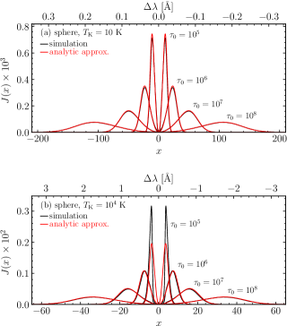
Figure 2.— Emergent Ly$\alpha$ spectra from a static, homogeneous sphere at (a) $T_{{\rm K}}=10$ K and (b) $10^{4}$ K, with different optical depths ($\tau_{0}=10^{5}-10^{8}$). The black curves are line profiles calculated with LaRT. The red curves denote the new analytic solution given in Appendix C, which was derived from the series solution of Dijkstra et al. (2006).

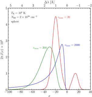
Figure 3.— Emergent Ly$\alpha$ for the dynamic motion test cases, in which the gas expands isotropically, and has a temperature of $T_{{\rm K}}=10^{4}$ K and a column density of $N_{{\rm HI}}=2\times 10^{20}$ cm^-2. The maximum velocity $v_{{\rm max}}$ of the Hubble-like outflow is denoted in units of km s^-1. The ordinate is the mean intensity integrated over the solid angle outgoing from the spherical surface.

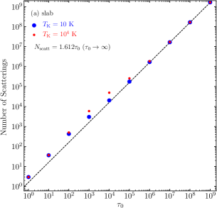
Figure 4.— Number of scatterings for (a) slab and (b) sphere as a function of the central optical depth $\tau_{0}$. The blue and red circles denote the cases of $T_{{\rm K}}=10$ K and $T_{{\rm K}}=10^{4}$ K, respectively. The black dashed lines denote the theoretical number of scatterings (a) $N_{{\rm scatt}}=1.612\tau_{0}$ and (b) $N_{{\rm scatt}}=0.958\tau_{0}$, which were derived at the limit of $\tau_{0}\rightarrow\infty$.

3. Tests of the Code

3.1. Static Media

As a test of our code, we performed the RT calculation for the cases of a static, plane-parallel slab, and sphere, for which Neufeld (1990) and Dijkstra et al. (2006), respectively, derived analytic approximations of the emergent mean intensity at the limit of large optical thickness. We also present new analytic formulae, which are slightly different from theirs, in Appendixes B and C. For these tests, we ignored the recoil effect unless otherwise stated; in other words, the recoil parameter $g_{*}$ in Equation (15) was assumed to be zero.

We first consider the infinite slab case in which the Ly$\alpha$ source is located at the mid-plane and injects monochromatic photons at frequency $x=0$ ($\nu=\nu_{\alpha}$). Figure 1 shows our simulation results for the slab with a temperature of (a) $T_{{\rm K}}=10$ K and (b) $T_{{\rm K}}=10^{4}$ K together with the approximate, analytic solution of Neufeld (1990). The optical thickness at line center ($\tau_{0}$) varies from $10^{5}$ to $10^{8}$, as indicated in the figure. Our results agree with the analytic solution, in general. However, as the optical thickness decreases and the temperature increases, the analytic solution begins to deviate from the simulation results. This discrepancy is because the analytic solution was derived in the limit of optically thick media ($2a\tau_{0}=9.4(T_{{\rm K}}/10^{4}{\rm K})^{-1/2}(\tau_{0}/10^{4})\gtrsim 10^{3}$).

As the second test, Figure 2 shows the simulation results for the case of a sphere in which photons are injected at frequency $x=0$ from the center of the sphere. The temperature of the medium is assumed to be (a) $T_{{\rm K}}=10$ K and (b) $T_{{\rm K}}=10^{4}$ K, and the optical depth at line center varies from $10^{5}$ to $10^{8}$, as for the slab geometry. In the figure, Equation (C3) given in Appendix C is compared. The analytic curves are in good agreement with the simulation results, except for $T_{{\rm K}}=10^{4}$ K and $\tau_{0}\lesssim 10^{6}$.

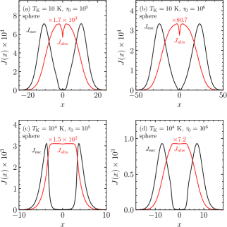
Figure 5.— Emergent and dust-absorbed Ly$\alpha$ spectra for a sphere. The gas temperature was assumed to be $T_{{\rm K}}=10$ K for the top panels (a) and (b), and $T_{{\rm K}}=10^{4}$ K for the bottom panels (c) and (d). The H I optical depth is $\tau_{0}=10^{5}$ for the left panels (a) and (c), and $\tau_{0}=10^{6}$ for the right panels (b) and (d). The black and red lines represent the emergent ($J_{{\rm esc}}$) and absorbed ($J_{{\rm abs}}$) spectra, respectively. The absorbed spectra were scaled up by multiplying a denoted number for clarity. The dust properties and gas-to-dust ratio of the Milky Way were adopted in the models. The absorption optical depths ($\tau_{{\rm abs}}$) are (a) $6.0\times 10^{-5}$, (b) $6.0\times 10^{-4}$, (c) $1.9\times 10^{-3}$, and (d) $1.9\times 10^{-2}$.

3.2. The Hubble-like flow

To test the code for the dynamic case, we examine the Hubble-like flow model. In the model, we consider an isothermal, homogeneous sphere, which is isotropically expanding or contracting. The bulk velocity of a fluid element at a distance $r$ from the center is assumed to be

$$\textbf{v}_{{\rm bulk}}(\mathbf{r})=\left(\frac{v_{{\rm max}}}{R}\right)\mathbf{r},$$ (33)

where $R$ is the radius of the medium and $v_{{\rm max}}$ is the maximum velocity at the edge of the sphere ($r=R$). There is no analytical solution of the emergent spectrum for a moving medium with non-zero temperature. We thus use the same parameters as the models of Laursen et al. (2009), Yajima et al. (2012), and Smith et al. (2017) and compare our simulation results with theirs. In the models, the gas medium is assumed to have a temperature of $T_{{\rm K}}=10^{4}$ K and a column density of $N_{{\rm HI}}=2\times 10^{20}$ cm^-2 (corresponding to $\tau_{0}\simeq 1.2\times 10^{7}$). The sphere of gas expands isotropically with $v_{{\rm max}}=20$, 200, or 2000 km s^-1. Figure 3 shows excellent agreement of our results with those of Laursen et al. (2009), Yajima et al. (2012), and Smith et al. (2017). We note that, as $v_{{\rm max}}$ increases, the blue peak is suppressed and disappears entirely at $v_{{\rm max}}\sim 200$ km s^-1. The peak location is also pushed further from the line center. These trends are because photons are Doppler shifted out of the line center due to the velocity gradient. However, at the extreme velocity of $v_{{\rm max}}=2000$ km s^-1, the peak approaches the line center again because the extreme velocity gradient allows photons to escape more easily. If a collapsing sphere ($v_{{\rm max}}<0$) is considered, then the red wing is suppressed, and the blue wing is enhanced, as opposed to the outflowing case.

3.3. Number of Scatterings

The average number of scatterings of Ly$\alpha$ experienced before escaping from the gas cloud is also an interesting quantity to examine. Figures 4(a) and (b) show the average number of scatterings for the infinite slab and sphere, respectively, as a function of the central optical thickness $\tau_{0}$. We calculated the number of scatterings in the cases of the gas temperature $T_{{\rm K}}=10$ K (blue circles) and $T_{{\rm K}}=10^{4}$ K (red dots) for a wide range of optical thickness $\tau_{0}=1-10^{9}$. The results cover the widest range reported to date. Overplotted as black dashed lines are the theoretical prediction (a) for the slab geometry (Equation (31)) and (b) for the spherical geometry (Equation (32)).

It is evident that the mean number of scatterings in the slab is higher than that in the sphere, because the slab geometry is infinitely extended along the XY plane and thus photons can escape only in the direction perpendicular to the XY plane.We also note that, in the optical thickness range of $10^{2}\lesssim\tau_{0}\lesssim 10^{6}$, Ly$\alpha$ photons in the lower-temperature medium undergo less scattering than in the higher-temperature medium. This is not caused by poor statistics; we increased the number of photon packets from $10^{5}$ up to $10^{9}$ and found no significant differences in the results.

Note that the mean numbers of scatterings for $\tau_{0}=10^{4}$ and $10^{5}$ in the bottom left panel of Figure 1 in Dijkstra et al. (2006) are lower than our results as well as the analytic approximation. This may be due to Dijkstra et al. (2006) having used the weighting scheme developed by Avery & House (1968), as described in Appendix B1 of Dijkstra et al. (2006). The distribution of the number of scatterings has a long tail to a large number of scatterings. The weighting scheme gives less weight to the photons that experience a large number of scatterings and thus underestimates the average number of scatterings.

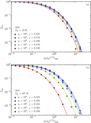
Figure 6.— Escape fraction $f_{{\rm esc}}$ of Ly$\alpha$ photons from a dusty, infinite slab with a temperature (a) $T_{{\rm K}}=10$ K and (b) $T_{{\rm K}}=10^{4}$ K as a function of $(a\tau_{0})^{1/3}\tau_{{\rm abs}}$. The escape fraction was calculated for the H I optical depths of $\tau_{0}=10^{4}-10^{8}$, and by varying the dust absorption optical depth $\tau_{{\rm abs}}$. The escaped fraction is fairly well represented by Equation (34) with different $\zeta$ values for different optical depths and temperatures, as denoted. The function with $\zeta=0.525$, as given in Neufeld (1990), is shown for the highest optical depth of $\tau_{0}=10^{8}$.

3.4. Dust Effect and Escape Fraction

So far, dust is neglected in the tests. The presence of dust grains in the medium suppresses the Ly$\alpha$ intensity escaping from the medium. Figure 5 shows the emergent spectra ($J_{{\rm esc}}$) from a dusty, homogeneous sphere of which the gas-to-dust ratio is that of the Milky Way ($\sim 100$ by mass). The spectra were obtained for four combinations of the gas temperature ($T_{{\rm K}}=10$ and $10^{4}$ K) and the optical thickness ($\tau_{0}=10^{5}$ and $10^{6}$). As shown in the figure, the overall shape of the emergent Ly$\alpha$ spectrum is not significantly altered by dust. In the figure, we also show the spectra of photons that are absorbed by dust ($J_{{\rm abs}})$. The absorbed spectra are not observable but may be useful when calculating the heating of dust grains in the vicinity of H II regions by Ly$\alpha$ photons.

It is worthwhile to note that there is a spiky dip feature at the line center of the dust-absorption spectra for the gas of $T_{{\rm K}}=10$ K. The feature indicates that Ly$\alpha$ photons are less absorbed at the very line core than at the outside of the core. Verhamme et al. (2006) also found a similar dip feature, as shown in Figure 3 in their paper, but it is much broader and deeper than ours. We found that the dip is noticeable only when the optical depth and temperature are rather low. As the optical depth and temperature increase, the dip feature is found to be smeared out and eventually disappear in the absorbed spectra. The dip feature is discussed in more detail in Appendix 32.

We also estimated the escape fraction of Ly$\alpha$ photons from a dusty, infinite slab. Neufeld (1990) derived an analytic equation for the escape fraction at a limit of large optical depths, as follows:

$$f_{{\rm esc}}=\left.1\right/\cosh\left[\frac{\sqrt{3}}{\pi^{5/2}\zeta}\left\{\left(a\tau_{0}\right)^{1/3}\tau_{{\rm abs}}\right\}^{1/2}\right].$$ (34)

He estimated $\zeta\approx 0.525$ by comparing this equation with numerical results of Hummer & Kunasz (1980), obtained for $\tau_{0}=5\times 10^{7}$ and $a=4.7\times 10^{-2}$ (or equivalently $T_{{\rm K}}=1$ K). Figure 6 shows the escape fraction as a function of $(a\tau_{0})^{1/3}\tau_{{\rm abs}}$ calculated for $\tau_{0}=10^{4}-10^{8}$ and $T_{{\rm K}}=10$, $10^{4}$ K. The dust optical thickness was varied so that $(a\tau_{0})^{1/3}\tau_{{\rm abs}}$ ranges from $10^{-2}$ to $10^{2}$. To compare our results with those of others, we assumed the dust scattering albedo of 0.5 and isotropic scattering ($g=0$). It appears that Equation (34) with $\zeta=0.525$ is indeed a good approximation for the cases of $\tau_{0}>10^{7}$. However, $\zeta=0.525$ overpredicts the escape fraction when the optical depth is lower than $10^{7}$. From the figure, it is also clear that $\zeta\approx 0.525$ is more adequate for lower temperature. This is because the equation was derived under the condition of $(a\tau_{0})^{1/3}>\tau_{{\rm abs}}$ and the width ($a$) of the Voigt profile is proportional to $T_{{\rm K}}^{-1/2}$. However, adopting a different value of $\zeta$ for different temperature $T$ and optical depth $\tau_{0}$, we found that the equation still provides a reasonably good representation of the escape fraction even when the condition required for the equation is not satisfied. The $\zeta$ values suitable for different temperatures $T_{{\rm K}}$ and optical depths $\tau_{0}$ are shown in Figure 6.

Figure 7.— Scattering rate $P_{\alpha}$ for a slab at the temperature of (a) $T_{{\rm K}}=10$ K and (b) $T_{{\rm K}}=10^{4}$ K. The scattering rates for $\tau_{0}=10^{3}$ and $10^{7}$ are shown in each panel. The black lines represent $P_{\alpha}$ calculated from Monte-Carlo simulations by directly counting the number of scatterings. The red dots are those calculated using the spectrum $J_{x}(0)$ obtained from the simulations. The green dashed lines denote the analytical solution, which overlaps with the simulation results for $\tau_{0}=10^{7}$. We also note that the simulation results for $\tau_{0}\gtrsim 10^{5}$ in (a) and $\tau_{0}\gtrsim 10^{6}$ in (b), but not shown here, almost coincide with the results for $\tau_{0}=10^{7}$.

Figure 8.— Scattering rate $P_{\alpha}$ for a sphere at the temperature of (a) $T_{{\rm K}}=10$ K and (b) $T_{{\rm K}}=10^{4}$ K. The scattering rates for $\tau_{0}=10^{3}$ and $10^{7}$ are shown in each panel. The black lines represent $P_{\alpha}$ calculated from Monte-Carlo simulations by directly counting the number of scatterings. The red dots are those calculated using the spectrum $J_{x}(0)$ obtained from the simulations. The green dashed lines denote the analytical solution, which overlap with the simulation results for $\tau_{0}=10^{7}$. The simulation results for $\tau_{0}\gtrsim 10^{5}$ in (a) and $\tau_{0}\gtrsim 10^{6}$ in (b) almost coincide with the results for $\tau_{0}=10^{7}$.

4. THE WF EFFECT IN SIMPLE GEOMETRIES

In this section, we present our main results that are relevant to the WF effect but calculated in simple geometries such as a uniform, infinite slab, and a sphere. We also compare the simulation results with the new analytic formulae derived in Appendixes B and C.

4.1. Scattering Rate

We present the scattering rate obtained for an unit generation rate of Ly$\alpha$ photons. Figure 7 compares the scattering rate calculated through a Monte-Carlo RT simulation and that obtained using an analytic approximation for the slab geometry. The results for the sphere geometry are shown in Figure 8. In the figures, the solid black lines represent the scattering rate calculated by directly counting the scattering events in the simulation. The red dots were estimated using the Ly$\alpha$ spectrum at the line center $J_{x}(x=0)$ and Equation (27). The green dashed lines denote the analytical, approximate solutions at the limit of a large optical thickness. The approximate formulae for the scattering rate in slab and sphere geometries are, respectively, obtained by combining Equations (B) and (C) for $J_{x}(0)$ with Equation (27). Note that the analytic solutions overlap with the simulation results for $\tau_{0}=10^{7}$ and are barely distinguishable in the figures.

The functional shape of $P_{\alpha}$ as a function of $\tau/\tau_{0}$ is more or less independent of the gas temperature and total optical thickness $\tau_{0}$. However, its absolute strength is proportional to $T_{{\rm K}}^{-1/2}$, as shown in Equation (27). Therefore, in Figures 7 and 8, the scattering rate $P_{\alpha}$ at $T_{{\rm K}}=10$ K is greater than that at $T_{{\rm K}}=10^{4}$ K by a factor of $\sim 31$.6 for a given optical depth $\tau_{0}$. We also note that the functional form of $P_{\alpha}$ in a sphere is much steeper than that in a slab. This tendency is due to photons in an infinite slab being able to escape the medium only through one direction that is perpendicular to the slab.

As $\tau_{0}$ increases, the scattering rate $P_{\alpha}(\tau/\tau_{0})$ gradually decreases and converges to an asymptotic form, which is well represented by the analytic formulae denoted by the green dashed lines in Figures 7 and 8. The convergence is achieved at a lower optical thickness when the medium has a lower temperature. As denoted in the figures, good agreement between the formula and simulation was obtained at $\tau_{0}\gtrsim 10^{5}$ for $T_{{\rm K}}=10$ K, but at a slightly higher optical depth of $\tau_{0}\gtrsim 10^{6}$ for $T_{{\rm K}}=10^{4}$ K. A similar trend can be also found in Figure 4, where the average number of scatterings begins to approach the asymptotic solution at a lower optical depth when the medium is in a lower temperature ($T_{{\rm K}}=10$ K) than in a higher temperature ($T_{{\rm K}}=10^{4}$ K).

The scattering rate $P_{\alpha}$ is affected by the presence of dust grains in the medium as well as by the systematic, bulk motion of the gas. Figure 9 shows the dependence of $P_{\alpha}$ on the dust-absorption optical depth in a slab. In the figure, the gas temperature and optical depth are $T_{{\rm K}}=10^{4}$ K and $\tau_{0}=10^{7}$, respectively, and the dust-absorption optical depth varies from $\tau_{{\rm abs}}=0$.0 (no dust) to $\tau_{{\rm abs}}=0.24$. These results were adopted from the models calculated for Figure 6. As expected, when $\tau_{{\rm abs}}$ gradually increases, $P_{\alpha}$ begins to drop. We note that, if the gas-to-dust ratio of the Milky Way is assumed, the absorption optical depth of the medium with $T_{{\rm K}}=10^{4}$ K and $\tau_{0}=10^{7}$ is $\tau_{{\rm abs}}=0.14$. This value is similar to the second-highest $\tau_{{\rm abs}}$ in Figure 9, indicating that dust grains effectively absorb Ly$\alpha$ photons and reduce the number of Ly$\alpha$ scatterings at a location of $\tau/\tau_{0}=0.5$ by a factor of $\sim 10$.

Figure 10 shows the effect of outflow on the scattering rate. In the figure, we assumed a Hubble-like, expanding sphere with a temperature of $T_{{\rm K}}=100$ K and an optical depth of $\tau_{0}=10^{3}$. The maximum velocity is increased from $v_{{\rm max}}=0$ to 10 km s^-1. As expected, the scattering rate rapidly decreases as the expansion velocity rises. Figures 9 and 10 illustrate how dramatically the number of scatterings can be reduced by the presence of dust and the bulk motion of the gas.

Figure 9.— Dependence of the scattering rate on the dust absorption optical depth of a slab. The gas kinetic temperature and H I optical depth are assumed to be $T_{{\rm K}}=10^{4}$ K and $\tau_{0}=10^{7}$, respectively, which corresponds to $(a\tau_{0})^{1/3}=16.77$. The dust-absorption optical depth varies from 0.0 (the uppermost) to 0.24 (the lowest).

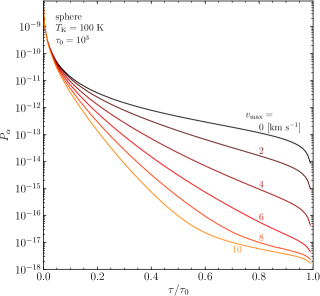
Figure 10.— Dependence of the scattering rate on the maximum velocity in a Hubble-like expanding, spherical medium with $T_{{\rm K}}=100$ K and $\tau_{0}=10^{3}$. The maximum expanding velocity varies from 0 km s^-1 (the uppermost) to 10 km s^-1 (the lowest).

4.2. Ly$\alpha$ Line Profile inside the Medium

We first examine the line profile of Ly$\alpha$ formed within a spherical medium when the recoil effect is ignored, i.e., $g_{*}=0$ in Equation (15). Figures 11 and 12 show the line profiles at various radial locations of a spherical medium with a temperature of $T_{{\rm K}}=10$ and $10^{4}$ K, respectively. In each figure, the results for two different optical depths ($\tau_{0}=10^{5}$ and $10^{7}$ in Figure 11, and $\tau_{0}=10^{6}$ and $10^{7}$ in Figure 12) are shown. The black lines in the figures denote the simulation results, while the red lines show the analytic solutions given in Equation (C3). It is clear that the approximate formula reproduces the simulation results reasonably well, in particular, when the optical depth is large enough, i.e., $\tau_{0}\gtrsim 10^{7}$ and the gas temperature is low ($T_{{\rm K}}=10$ K). For $T_{{\rm K}}=10^{4}$ K and $\tau_{0}<10^{6}$, however, the analytic solution significantly underestimates the intensity. We also note that the analytic solution tends to underestimate the Ly$\alpha$ intensity in the central portion and overestimate in outer parts. The same trend was found by Higgins & Meiksin (2012) who solved the moment equations numerically. We also found a similar trend for a slab, but not shown in this paper. It should also be mentioned that the Ly$\alpha$ spectrum evolves progressively to a typical double-peak shape as upon approaching the system boundary ($\tau/\tau_{0}\gtrsim 0.95$), but not clearly shown in the figures.

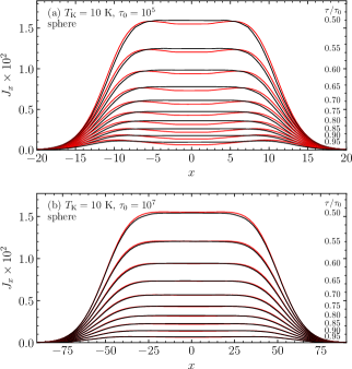
Figure 11.— Spectra of the Ly$\alpha$ radiation field at various radial locations (corresponding to $\tau/\tau_{0}=$ 0.50, 0.55, $\cdots$, 0.95) in a spherical medium with a temperature of $T_{{\rm K}}=10$ K. No recoil effect is taken into account so that the line center is flat. The optical depth at line center is (a) $\tau_{0}=10^{5}$ and (b) $\tau_{0}=10^{7}$. Black lines show our simulation results and red lines are from the analytical approximation of Equation (C3).

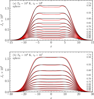
Figure 12.— Spectra of the Ly$\alpha$ radiation field at various radial locations (corresponding to $\tau/\tau_{0}=$ 0.50, 0.55, $\cdots$, 0.95) in a spherical medium with a temperature of $T_{{\rm K}}=10^{4}$ K. No recoil effect is taken into account so that the line center is flat. The optical depth at line center is (a) $\tau_{0}=10^{6}$ and (b) $\tau_{0}=10^{7}$. Black lines show our simulation results and red lines are from the analytical approximation of Equation (C3).

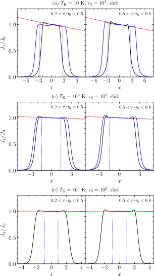
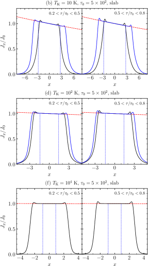
Figure 13.— Recoil effect on the Ly$\alpha$ radiation field within a slab. The gas has a temperature of (a)(b) $T_{{\rm K}}=10$ K, (c)(d) $T_{{\rm K}}=10^{2}$ K, and (e)(f) $T_{{\rm K}}=10^{4}$ K. The optical depth at line center is (a)(c)(e) $\tau_{0}=10^{2}$ and (b)(d)(f) $\tau_{0}=5\times 10^{2}$. The figures show the spectra in linear scale. The black solid lines represent the spectra obtained when the fine structure was ignored, while the blue solid lines were obtained after taking it into account. The blue dotted lines denote the frequency interval $|x|\leq x_{*}$. Here, $x_{*}=0.84+\left|\nu_{{\rm K}}-\nu_{{\rm H}}\right|/2\Delta\nu_{{\rm D}}$ for (a) to (d), and $x_{*}=0.84$ for (e) and (f).

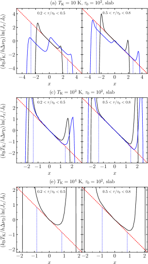
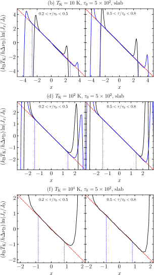
Figure 14.— Recoil effect on the Ly$\alpha$ radiation field within a slab. The same as Figure 13 except that the spectra are shown in logarithmic scale. The gas has a temperature of (a)(b) $T_{{\rm K}}=10$ K, (c)(d) $T_{{\rm K}}=10^{2}$ K, and (e)(f) $T_{{\rm K}}=10^{4}$ K. The optical depth at line center is (a)(c)(e) $\tau_{0}=10^{2}$ and (b)(d)(f) $\tau_{0}=5\times 10^{2}$.

Figure 15.— Ly$\alpha$ line profiles in an expanding medium with $v_{{\rm max}}=5$ km s^-1, $T_{{\rm K}}=100$ K, and $\tau_{0}=10^{3}$. The spectra are shown at optical depths of $\tau/\tau_{0}=0.0,$ 0.2, 0.4, 0.6, 0.8, and 1.0. They were normalized by the maximum intensities for convenience.

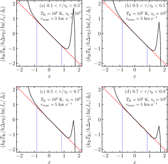
Figure 16.— Thermalization of the Ly$\alpha$ line profiles inside an expanding medium with $v_{{\rm max}}=5$ km s^-1. The model is the same as in Figure 15, but the line profiles are shown in logarithmic scale for four optical depth bins.

We next consider the case in which the atomic recoil effect is taken into account in the simulation. Figure 13 shows the Ly$\alpha$ spectra in a static, infinite slab for six different sets of physical parameters. The gas temperature is assumed to be $T_{{\rm K}}=10$ K in Figures 13(a) and (b), while it is $T_{{\rm K}}=10^{2}$ K in Figures 13(c) and (d), and $T_{{\rm K}}=10^{4}$ K in Figures 13(e) and (f). The optical thickness for the system is $\tau_{0}=10^{2}$ for Figures 13(a), (c), and (e), and $\tau_{0}=5\times 10^{2}$ for Figures 13(b), (d), and (f). In each figure, the left panels show the Ly$\alpha$ spectra measured in an optical depth bin of $0.2<\tau/\tau_{0}<0.5$; the right panels show the spectra in $0.5<\tau/\tau_{0}<0.8$.

As noted in Section 2.3, the frequency gap between the fine-structure levels of the $n=2$ state can be comparable to the line width formed in the medium with a relatively low optical depth and low temperature (i.e., $T_{{\rm K}}\lesssim 10^{2}$ K). In Figures 13(a) to (d), we, therefore, show also the Ly$\alpha$ spectra obtained when the fine structure is considered. In the figures, the black and blue solid lines denote the Ly$\alpha$ spectra calculated when the fine structure is ignored and taken into consideration, respectively. In Figure 13(a) for $\tau_{0}=10^{2}$, we see that the spectra, denoted in blue, show two steps due to the fine structure. However, as the optical thickness increases higher than $\tau_{0}\approx 5\times 10^{2}$, the step-like shape disappears, as shown in Figure 13(b) for $\tau_{0}=5\times 10^{2}$. The intensity ratio of the doublet line becomes 1:1 at high optical depths as a result of a considerable number of resonance scatterings, and thus the step signature of the doublet disappears. The step shape disappeared at a lower optical depth as temperature increases. For instance, in the case of $T_{{\rm K}}=10^{2}$ K (Figure 13(c)), the step shape is not found already at $\tau_{0}=10^{2}$.

The most notable thing in Figures 13(a) to (d) is that the Ly$\alpha$ spectra are tilted in the central part, unlike those shown in Figures 11 and 12 in which no recoil effect was considered. To compare with the expectation in the WF effect theory, we overlay an exponential function $\exp\left[-h(\nu-\nu_{\alpha})/k_{{\rm B}}T_{{\rm K}}\right]$ for the gas temperature $T_{{\rm K}}$ with a red dashed line. As shown in the figures, the spectra clearly appears to be consistent with the function expected for the WF effect. However, in Figures 13(e) and (f) for the highest temperature of $T_{{\rm K}}=10^{4}$ K, the spectral shape appears to be nearly constant at the central part. In fact, the exponential function for a high $T_{{\rm K}}$ is almost constant. Hence, at first glance, it seems that it is not possible to confirm whether the Ly$\alpha$ spectra within the medium at a high temperature follow an expected functional form or not.

However, we note that the spectrum can be expressed by

$$\frac{k_{{\rm B}}T_{{\rm K}}}{h\Delta\nu_{{\rm D}}}\ln\left(J_{x}/J_{0}\right)=-x.$$ (35)

Thus, if the spectrum is drawn in logarithmic scale, as in the left side of the above equation, and compared with $-x$, we can readily illustrate that the spectrum follows the expected function. Figure 14 compares the Ly$\alpha$ spectra represented in logarithmic scale with $-x$, which is indicated by the dashed red line, for all cases shown in Figure 13. Consequently, we conclude that the Ly$\alpha$ spectrum is well described by an exponential function with a slope of the gas temperature, even at the highest temperature ($T_{{\rm K}}=10^{4}$ K) presented here. Interestingly, Figures 13(a) and 14(a) show that the double steps (blue lines) have the same exponential slope corresponding to the gas temperature, although they are disconnected.

Here, we note that the exponential shape should remain valid across the frequency interval corresponding to the width of the resonance profile $\phi_{x}$, i.e., $|x|\lesssim x_{*}=0.84\ (=\ln 2)$. In this paper, we take this width as the full-width at half maximum (FWHM) of the Voigt function for $a\ll 1$, or equivalently the FWHM of the Gaussian function with a standard deviation of $1/\sqrt{2}$. If we additionally consider the line splitting due to the fine structure, the exponential shape should be kept over the whole range of the frequency gap of the doublet plus the width of the resonance profile, i.e., $|x|\lesssim x_{*}=0.84+|\nu_{\nicefrac{{3}}{{2}}}-\nu_{\nicefrac{{1}}{{2}}}|/(2\Delta\nu_{{\rm D}})$. Otherwise, the 21-cm spin temperature could not approach the gas temperature. Note that $|\nu_{\nicefrac{{3}}{{2}}}-\nu_{\nicefrac{{1}}{{2}}}|/(2\Delta\nu_{{\rm D}})=5.83\times 10^{-2}\left(T_{{\rm K}}/10^{4}\,\text{K}\right)^{-1/2}$. In order to check if this is the case, the vertical blue dashed lines are overlaid in Figures 13 and 14 (and in other figures as well where necessary) to denote the frequency interval $|x|\leq x_{*}$.

In the case of $T_{{\rm K}}=10$ K and $\tau_{0}=10^{2}$ shown in Figure 14(a), it appears that the spectral shape does not satisfy the requirement because of the discontinuous step feature. On the other hand, we found that the spectra obtained for $\tau_{0}\gtrsim 3\times 10^{2}$ and $T_{{\rm K}}=10$ K follows the required exponential shape over the frequency interval $|x|\leq x_{*}$, for instance, as shown in Figure 14(b). In the case of $T_{{\rm K}}=10^{2}$ K ($\tau_{0}=10^{2}$ and $\tau_{0}=5\times 10^{2}$), the desired profile is more clearly seen in Figures 14(c) and (d). Figures 14(e) and (f) also show that the line profiles follow the expected shape very well, over the frequency interval $|x|\leq x_{*}$, even for the highest temperature $T_{{\rm K}}=10^{4}$ K. We examined many different cases and found that the necessary condition for the Ly$\alpha$ spectral profile is fulfilled at an optical depth as low as $\tau_{0}\simeq(1-5)\times 10^{2}$. In general, as the temperature is low, it appeared that the requirement is satisfied at a lower optical depth. If the optical depth is lower than $\tau_{0}\simeq 10^{2}$, the Ly$\alpha$ spectrum was, in general, not fully thermalized in the temperature range of $10\,\text{K}\leq T_{{\rm K}}\leq 10^{4}\,\text{K}$, examined in this paper.

The above results were obtained in static media. It would, therefore, be worthwhile to examine whether the Ly$\alpha$ spectrum will have a shape of the required exponential function in a medium in motion. For instance, we show the spectra within a Hubble-like, expanding medium in Figures 15 and 16. Both figures were obtained for an expanding medium with $\tau_{0}=10^{3}$, $T_{{\rm K}}=10^{2}$ K. Figure 15 shows the Ly$\alpha$ spectra at several locations, expressed in terms of optical depth, in a spherical medium with a maximum expanding velocity of $v_{{\rm max}}=5$ km s^-1. In Figure 15, the spectra near the line center ($x=0$) seem flat. However, more detailed views in Figure 16 clearly illustrate that the spectra calculated at various optical depth bins follow the exponential function for $T_{{\rm K}}=10^{2}$ K. We, therefore, can conclude that the Ly$\alpha$ line profile follows the desired exponential function with a slope corresponding to the gas temperature even in an expanding medium, if the expanding velocity is not too fast. If a medium rapidly expands or, more precisely, has a velocity gradient, across a region with an optical thickness of $\tau_{0}\approx 100-500$, larger than the thermal velocity dispersion, Ly$\alpha$ photons will escape the region before they fully develop the spectral shape required for the WF effect. The relevant issue in moving media is further addressed in the next section.

The initial frequency of Ly$\alpha$ was fixed at $\nu=\nu_{\alpha}$ ($x=0$) for the above discussion. The same conclusion was obtained even when we assumed a Voigt profile or a flat continuum. The Ly$\alpha$ line is broadened or adjusted very quickly in a medium with an optical thickness of $\tau_{0}\gtrsim 10^{2}$ so that the initial frequency distribution did not significantly alter the resulting spectra; only the spectra in the vicinity of the source showed a weak dependence on the initial frequency distribution.

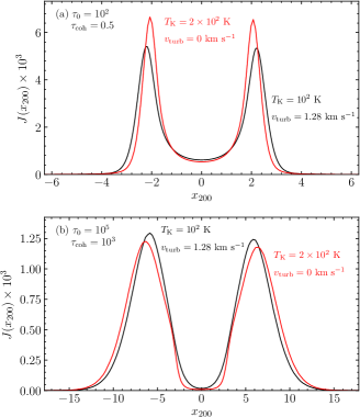
Figure 17.— Turbulence effect on the Ly$\alpha$ line profile emerging from a sphere with the central optical depth (a) $\tau_{0}=10$ and (b) $\tau_{0}=10^{5}$. The black lines are the spectra emerging from a sphere with $T_{{\rm K}}=10^{2}$ K when random turbulent motion with $v_{{\rm turb}}=1.28$ km s^-1 is applied. The red lines were obtained when no random turbulent motion was taken into consideration, but the temperature of the medium was assumed to be $T_{{\rm K}}=2\times 10^{2}$ K, corresponding to the Doppler temperature $T_{{\rm D}}$, defined in Equation (36). All spectra are shown as functions of the same relative frequency $x_{T}$, which is defined for $T_{{\rm K}}=200$ K, for ease of comparison.

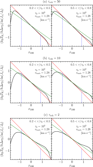
Figure 18.— Turbulence effect, when the coherence scale of optical depth varies, on the Ly$\alpha$ line profile in a spherical medium with the central optical depth $\tau_{0}=10^{3}$ and temperature $T_{{\rm K}}=10^{2}$ K. From the top to bottom panels, the coherence scale decreases from $\tau_{{\rm coh}}=50$ to 2. The red dashed lines represent the exponential function for $T_{{\rm K}}=10^{2}$ K, while the green dashed lines are for $T_{{\rm K}}=200$ K.

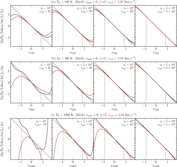
Figure 19.— Ly$\alpha$ line profiles in a multiphase medium in which three kinetic temperatures ($T_{{\rm K}}=$ 100, 500, and 1000 K) are equally mixed. The central optical depth was assumed to be $\tau_{0}=10^{3}$, $5\times 10^{3}$, $10^{4}$, and $5\times 10^{4}$ from left to right. The coherence optical depth is $\tau_{{\rm coh}}=10$, $50$, $10^{2}$, and $5\times 10^{2}$, respectively, from the first to fourth column. The red dashed lines denote the exponential functions for (a) $T_{{\rm K}}=100$ K, (b) 500 K, and (c) 1000 K. The black lines show the Ly$\alpha$ line profiles when there is no random motion was applied while the red lines represent the models that include a random, turbulent motion with a velocity dispersion of $v_{{\rm turb}}=4.06$ km s^-1.

4.3. Turbulence Effect on Line Profile

In the above calculation of the Ly$\alpha$ RT, only the thermal motion and systematic bulk flow of gas were taken into account. Aside from the thermal broadening, the line width of Ly$\alpha$ may also be broadened by the presence of the turbulent velocity field. It is convenient to define the Doppler temperature $T_{{\rm D}}$ as in Liszt (2001), to incorporate the turbulence effect (see also Draine, 2011):

$$2k_{{\rm B}}T_{{\rm D}}/m_{{\rm H}}=2k_{{\rm B}}T_{{\rm K}}/m_{{\rm H}}+v_{{\rm turb}}^{2},$$ (36)

where $v_{{\rm turb}}$ is the velocity dispersion of turbulent motion. The Doppler parameter $b$ defined by

$$b=\sqrt{v_{{\rm th}}^{2}+v_{{\rm turb}}^{2}}$$ (37)

is also useful to describe effects caused by the turbulent motions, as in Verhamme et al. (2006). The Doppler temperature $T_{{\rm D}}$ (or Doppler parameter $b$) has been used in place of the thermal kinetic temperature (or thermal velocity) to describe the Ly$\alpha$ spectral shape. However, it has not been verified whether this prescription of incorporating the turbulent fluid motion is appropriate in the context of Ly$\alpha$ RT, especially with regards to the WF effect. Hydrodynamic simulations for galaxies, where the turbulence effects are included, have been adopted to calculate the emergent Ly$\alpha$ spectra. However, in these studies, the turbulence effect could not be separated from the pure thermal motion effect.

Before we go forward, we need to classify random or turbulent motions into two categories, microturbulence and macroturbulence, as described in Leung & Liszt (1976). Microturbulence is used to refer to the case in which the correlation length of the velocity field (or the size of a typical turbulent element) is small compared with the photon mean free path. Macroturbulence refers to the case in which the scale length of the turbulent fluctuations is large enough compared with the mean free path of photons. In the context of the WF effect, we need to compare the correlation length with a length corresponding to $\tau_{0}\approx 100-500$, instead of the mean free path, which is required to make the color temperature equal to the kinetic temperature.

In this paper, to quantify the degree of spatial coherence (or correlation) of the medium, we define the coherence length as the size over which the physical quantities, such as density, temperature, and bulk motion, remain uniform. We also define the coherence optical depth as an optical depth corresponding to the coherence length. In our simulation, each cell has a constant density, temperature, and bulk motion velocity and thus the coherence length (or optical depth) is the size (optical depth) of individual cells. In the following models, we utilize a 3D Cartesian box to implement spherical geometry by setting the density zero outside of a certain radius.

First, we examine how the random, turbulence motion affects the emergent Ly$\alpha$ spectrum by adopting a simple, random motion model to mimic turbulence. We employ a random, 3D velocity field in which three velocity components in each cell are independently produced to follow a Gaussian distribution with a standard deviation of $v_{{\rm turb}}/\sqrt{2}$. According to the above prescription to describe the turbulence effect, the emergent spectrum from a medium with a kinetic temperature $T_{{\rm K}}$ and having a Gaussian random motion with a velocity dispersion $v_{{\rm turb}}$ is supposed to be equivalent to that obtained from a medium with a gas temperature of $T_{{\rm D}}=\left(T_{{\rm K}}+m_{{\rm H}}v_{{\rm turb}}^{2}/2k_{{\rm B}}\right)^{1/2}$, but with no turbulence motion.

In Figure 17, we show the results for $T_{{\rm K}}=10^{2}$ K, $v_{{\rm turb}}=1.28$ km s^-1, and $T_{{\rm D}}=2\times 10^{2}$ K. In the figure, the spectrum emerging out of a medium with the turbulence motion is denoted in black, and the emergent spectrum from a medium with only the pure thermal motion corresponding to the Doppler temperature $T_{{\rm D}}$ in red. The medium is assumed to have an optical depth of $\tau_{0}=10^{2}$ and $\tau_{0}=10^{5}$, respectively, in Figures 17(a) and 17(b). The coherence optical depth is taken to be $\tau_{{\rm coh}}=0.5$ for the case of optical depth $\tau_{0}=10^{2}$ and $\tau_{{\rm coh}}=10^{3}$ for $\tau_{0}=10^{5}$; in other words, the number of cells in the simulation box is $400^{3}$ for Figure 17(a) and $200^{3}$ for Figure 17(b). Thus, Figure 17(a) illustrates the case of microturbulence and Figure 17(b) macroturbulence. When dealing with several models in which turbulent motion or many different velocities are concerned, we need to use a common abscissa in the spectra. We use $x_{T_{{\rm K}}}$ to denote the relative frequency defined for the temperature $T_{{\rm K}}$; for instance, $x_{200}$ in Figure 17 represents the relative frequency defined when $T_{{\rm K}}=200$ K. In the figures, we find that the two results obtained using two different methods agree reasonably well with each other; therefore, the commonly adopted prescription provides an excellent method to predict the emergent Ly$\alpha$ spectrum from a turbulent medium regardless of the coherence length.

Second, we investigate the turbulence effect on the Ly$\alpha$ spectrum measured inside the medium. We calculated the Ly$\alpha$ radiation field spectra in a spherical medium with $T_{{\rm K}}=10^{2}$ K and $\tau_{0}=10^{3}$. The turbulent velocity is again $v_{{\rm turb}}=1.28$ km s^-1, and the coherence optical depth was adjusted to be $\tau_{{\rm coh}}=50$, 10, and 2 by varying the cell size (or the number of cells of the system). Figure 18 shows the spectra at two radial distance intervals corresponding to $0.2<\tau/\tau_{0}<0.5$ and $0.5<\tau/\tau_{0}<0.8$ for each model. In the figure, the solid black lines represent the calculated Ly$\alpha$ spectra, and the red and green dashed lines denote exponential functions for $T_{{\rm K}}$ and $T_{{\rm D}}$, respectively. From Figure 18(a) ($\tau_{{\rm coh}}=50$) to 18(c) ($\tau_{{\rm coh}}=2$), the spectra gets shallower from $-x_{100}$ (for $T_{{\rm K}}$) to $-x_{100}/2$ (for $T_{{\rm D}}$). These results indicate that in the case of large coherence optical depths (macroturbulence), the color temperature is solely determined by the gas kinetic temperature; in other words, the prescription to incorporate turbulent motions is only valid for the microturbulence case ($\tau_{{\rm coh}}\ll\tau_{{\rm WF}}\approx 100$).

The ISM and IGM will not have a constant temperature, but rather a continuously varying temperature structure; this is called the multiphase medium. Thus, there would be a possibility that Ly$\alpha$ photons that were thermalized to one temperature in a volume element could then be perturbed or disturbed while they pass through an adjacent parcel with a different temperature. It may also be possible that the Ly$\alpha$ photons can be no longer characterized by the gas temperature of the volume element that the photons traverse. It is, therefore, worthwhile to examine whether thermalization can immediately occur after photons enter the next parcel with a different temperature.

To investigate this possibility in a multiphase medium, we used a uniform density medium and randomly assigned one of three temperatures of $T_{{\rm K}}=100$, 500, and 1000 K to every cell with an equal probability of $1/3$ and estimated the average spectra taken from the cells with each temperature. In Figure 19, we show the results (black lines) for $\tau_{0}=10^{3}$, $5\times 10^{3}$, $10^{4}$, and $5\times 10^{4}$ from the first to fourth column. For each optical depth, the top, middle, and bottom panels show the spectra of the phases with $T_{{\rm K}}=100$, 500, and 1000 K, respectively. Each cell has a size of optical depth of $\tau_{{\rm coh}}=\tau_{0}/100$, and thus, for instance, $\tau_{{\rm coh}}=10$ for the case of $\tau_{0}=10^{3}$ and $\tau_{{\rm coh}}=5\times 10^{2}$ for $\tau_{0}=5\times 10^{4}$. In the first and second columns ($\tau_{{\rm coh}}=10$ and $50$), we find that the Ly$\alpha$ spectrum is not thermalized to the gas temperature ($T_{{\rm K}}$) at all in the cells with the higher temperatures $T_{{\rm K}}=5\times 10^{2}$ and $10^{3}$ K; the spectrum is steeper than that expected, because of the influence of spectra having lower temperatures in adjacent cells. However, in the cells with the lowest temperature ($T_{{\rm K}}=100$ K), the spectrum is fully thermalized even at a coherence optical depth as low as $\tau_{{\rm coh}}=50$ (second column). For the intermediate temperature ($T_{{\rm K}}=500$ K) and $\tau_{{\rm coh}}=50$, the spectrum appears to have a color temperature that is slightly different from the gas temperature. These results are because the thermalization is achieved more quickly in a lower temperature medium than in a higher temperature medium. On the other hand, in the case of the higher optical depth of $\tau_{0}=5\times 10^{4}$, as shown in the rightmost panels, in which the optical depth of individual cells is $5\times 10^{2}$, the Ly$\alpha$ spectra are found to be fully thermalized to the gas temperatures in all cells regardless of the gas temperature.

In Figure 19, we also show the spectra (red solid lines) taken from the models in which a random velocity field with $v_{{\rm turb}}=4.06$ km s^-1 (corresponding to a temperature of 10³ K) was additionally applied to the same media. For low optical depths (first and second columns), the resulting Ly$\alpha$ line profiles show shallower slopes compared to those (black lines) obtained when no random, turbulent motion is employed. The shallow slopes are attributable to the influence of turbulent motion ($T_{{\rm D}}>T_{{\rm K}}$). However, even in this case, we find the same conclusion as before that thermalization is more readily achieved in high optical depths and low temperatures.

In summary, we conclude that the emergent spectrum from a turbulent medium becomes wider according to the commonly adopted prescription regardless of the coherence length. However, the color temperature of the Ly$\alpha$ radiation field within the turbulent medium approaches the gas temperature, as opposed to the common assumption, unless the coherence scale is too small. In most astrophysical environments, the Ly$\alpha$ optical depth would be very large for a turbulent length scale, as discussed in Section 6.2, and thus, we conclude that the color temperature in the WF effect theory should include only the gas temperature, but not the turbulence effect.

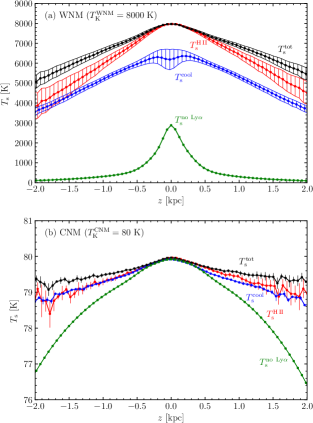
Figure 20.— Spin temperature for the Ferriere model at the solar vicinity (Ferriere, 1998). (a) Spin temperature distribution of the WNM as a function of height from the Galactic plane. (b) Spin temperature distribution of the CNM. Ly$\alpha$ photons were produced either from H II regions or cooling hot gas. The label “tot” indicates the model that includes both sources. The gas temperature assumed for each phase is also denoted in each panel. The hatch areas and error bars indicate the standard deviation of temperature at a given height. The abscissa values were slightly moved to clarify the data points. The green lines and dots denote the spin temperature when no Ly$\alpha$ pumping is taken into account.

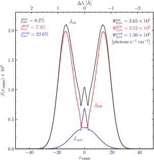
Figure 21.— The emergent Ly$\alpha$ spectra obtained from the Ferriere model. The Ly$\alpha$ production rate ($\Psi_{{\rm Ly}\alpha}$) and escape fraction ($f_{{\rm esc}}$) for each source (H II regions and cooling gas) are shown together with those for the combined model (“tot”).

5. THE WF EFFECTS IN ISM MODELS

In the previous section, we present basic properties of the Ly$\alpha$ RT with regard to the WF effect. We now apply our methods to more realistic ISM models that may be appropriate to the solar neighborhood in the Milky Way galaxy. We first describe the Ly$\alpha$ production mechanisms (Section 5.1) and the collisional transition rates for the H I hyperfine levels (5.2), which are required to examine the WF effect in the ISM models. We use two multiphase ISM models, (1) a rather idealized theoretical model for the vertical profiles of density and volume filling factors (Ferriere, 1998; Section 5.3) and (2) snapshots of a full 3D MHD simulation result (Kim & Ostriker, 2017; Section 5.4). The present results can be readily applied to other hydrodynamic models for whole galaxies.

5.1. Ly$\alpha$ Sources: Photoionization and Collisional Cooling

There are two primary mechanisms to produce Ly$\alpha$ photons. First, photoionization of hydrogen by the UV radiation field is followed by the recombination, leaving the atom in an excited state. The subsequent radiative cascades to the ground state can then produce a Ly$\alpha$ photon, which is often called the ‘fluorescent’ radiation in the Ly$\alpha$ astronomy community. H II regions that are photoionized by bright OB associations are the most prominent sources of Ly$\alpha$ photons in the ISM. Second, the collision between an electron and a hydrogen atom can excite or ionize the atom, and then the hydrogen produces a Ly$\alpha$ photon as the atom decays down to the ground state or recombines. This process is referred to as Ly$\alpha$ production via ‘cooling.’

Both Ly$\alpha$ sources are included in the following RT simulations. For the Ly$\alpha$ recombination photons, we inject initial Ly$\alpha$ photons near the Galactic plane smoothly following the vertical distribution of H II regions in the vicinity of the Sun. We adopt a Gaussian vertical distribution with a scale height of 81 pc, while the horizontal distribution is uniform. Ly$\alpha$ photons are injected with frequencies according to a Voigt profile for the H II region temperature of $T_{{\rm K}}=10^{4}$ K. Note that the initial photon frequency did not significantly alter our RT simulation results.

Vacca et al. (1996) estimated the production rate of ionizing UV photons (Lyman continuum; Lyc) from 429 O- and early B stars within 2.5 kpc of the Sun to be $\Psi_{{\rm Lyc}}=3.7\times 10^{7}$ photons cm^-2 s^-1. Each ionizing photon should produce $\sim 0.68$ Ly$\alpha$ photons in the case B condition. Hence, the production rate of Ly$\alpha$ photons by H II regions in the vicinity of the Sun is $\Psi_{{\rm Ly}\alpha}=2.52\times 10^{7}$ photons cm^-2 s^-1. The production rate is expressed by $\Psi_{{\rm Ly}\alpha}=\mathcal{L}_{*}/h\nu_{\alpha}$ in terms introduced in Section 2.5.

To calculate the Ly$\alpha$ production rate due to the collisional cooling, we assumed that the gas is in the collisional ionization equilibrium (CIE), in which the ionization fraction of hydrogen is calculated by balancing the collisional ionization rate with the case A recombination rate of hydrogen. The ionization and recombination rate coefficients of hydrogen are given in Equations (13.11) and (14.5), respectively, of Draine (2011). To calculate the electron density, we also included electrons produced by collisional ionization of helium. The collisional ionization fraction of helium was calculated using the collisional ionization and recombination rate coefficients provided in Cen (1992).

The total Ly$\alpha$ emissivity caused by the collisional excitation and ionization is given by

$$\frac{4\pi j_{{\rm Ly}\alpha}}{h\nu_{\alpha}}=n_{e}n_{{\rm H}}\frac{C_{{\rm Ly}\alpha}(T_{{\rm K}})}{h\nu_{\alpha}}+n_{e}n_{p}\alpha_{{\rm B}}P_{{\rm B}}({\rm Ly}\alpha),$$ (38)

where $n_{e}$, $n_{{\rm H}}$, and $n_{p}$ are the densities of electron, neutral hydrogen, and proton, respectively. We calculated the cooling rate coefficient $C_{{\rm Ly}\alpha}(T_{{\rm K}})$ via Ly$\alpha$ emission using version 9 of the CHIANTI spectral code (Dere et al., 1997, 2019), which we found to be well represented by

$$C_{{\rm Ly}\alpha}(T_{{\rm K}})=4.13\times 10^{-19}\exp\left(-\frac{117744}{T_{{\rm K}}}\right)\ \text{erg}\ {\rm cm^{3}}\ {\rm s}^{-1},$$ (39)

within 10% error in most cases and 20% error at the very most. The case B recombination rate coefficient $\alpha_{{\rm B}}$ is given in Equation (14.6) of Draine (2011). The probability $P_{{\rm B}}({\rm Ly}\alpha)$, as a function of gas temperature, that a recombination event leads to the production of a Ly$\alpha$ photon in the case B condition is given by Cantalupo et al. (2008).

5.2. Collisional Transition Rate of the Hyperfine Levels

The downward transition rate from the hyperfine level “1” to “0” due to particle collisions $P_{10}^{{\rm c}}$ in Equation (24) is the sum of the downward rates by all collision partners (hydrogen atoms, protons, and electrons). The downward rate associated with interactions with electrons and protons were taken from Liszt (2001). We adopted the formula given by Shaw (2005) for the downward transition rate arising from collisions with other hydrogen atoms.

5.3. The Ferriere Model

Ferriere (1998) describes a global model of the ISM in our Galaxy. The ISM comprises of two neutral media and two ionized media; the WNM and CNM, and the warm ionized medium (WIM) and hot ionized medium (HIM). The CNM has a temperature of 80 K, the WNM and WIM a temperature of 8000 K, and the HIM a temperature of $10^{6}$ K. Partial ionization is not considered in this model so that no free electrons coexist with the neutral hydrogen. Therefore, the recombination process that follows collisional ionization (WIM) or photoionization (H II regions) is the only Ly$\alpha$ source.

The space-averaged densities in the CNM, WNM, WIM, and HIM near the Sun are approximated, as a function of height $z$ perpendicular to the Galactic plane, by

$$\frac{\left\langle\rho_{{\rm CNM}}(z)\right\rangle}{\rho_{{\rm CNM}}^{0}} = 0.859e^{-\left(z/H_{1}\right)^{2}}+0.047e^{-\left(z/H_{2}\right)^{2}}+0.094e^{-\left|z\right|/H_{3}}$$

$$\frac{\left\langle\rho_{{\rm WNM}}(z)\right\rangle}{\rho_{{\rm WNM}}^{0}} = 0.456e^{-\left(z/H_{1}\right)^{2}}+0.403e^{-\left(z/H_{2}\right)^{2}}+0.141e^{-\left|z\right|/H_{3}}$$

$$\frac{\left\langle\rho_{{\rm WIM}}(z)\right\rangle}{\rho_{{\rm WIM}}^{0}} = 0.948e^{-\left|z\right|/1{\rm kpc}}+0.052e^{-\left|z\right|/150{\rm pc}}$$

$$\frac{\left\langle\rho_{{\rm HIM}}(z)\right\rangle}{\rho_{{\rm HIM}}^{0}} = 0.12+0.88e^{-\left|z\right|/1.5{\rm kpc}},$$

where the densities at the Galactic plane are $\rho_{{\rm CNM}}^{0}=0.340$ cm^-3, $\rho_{{\rm WNM}}^{0}=0.226$ cm^-3, $\rho_{{\rm WIM}}^{0}=0.025$ cm^-3, and $\rho_{{\rm HIM}}^{0}=4.8\times 10^{-4}$ cm^-3, and the three scaleheights are $H_{1}=0.127$ kpc, $H_{2}=0.318$ kpc, and $H_{3}=0.403$ kpc.

The volume filling factors, defined as the ratios of their space-averaged densities to their true densities, of the three phases (CNM, WNM, and WIM) are calculated using Equations (38) to (40) of Ferriere (1998), as functions of the filling factor of the HIM phase and the thermal pressures. The filling factor of the HIM phase at the solar position ($R=R_{\odot}$) is given as a function of height from the Galactic plane in Figure 12 of Ferriere (1998); we digitized the figure for the present work.

We used these relations to calculate the volume filling factors and true densities of the four phases at each vertical height bin. We then randomly assigned one of four phases to every volume element by comparing a random number with the given filling factors at that vertical height. The temperatures and true densities are then determined for each volume element. For this model, the simulation box was assumed to have a physical size of ($\pm 3$ kpc)³, and the number of volume elements was $100^{3}$. The periodic boundary condition along the $XY$ plane was implemented. The Ly$\alpha$ RT simulations were performed for H II regions and Ly$\alpha$ cooling sources, separately, to calculate the scattering rate $P_{\alpha}$ in every volume element. The spin temperature was then calculated using Equation (22).

Figure 20 shows the resulting average vertical profiles of spin temperature for the WNM and CNM phases, respectively, in the top and bottom panels. In the figure, we show the results when Ly$\alpha$ photons originating either from H II regions (red) or cooling hot gas (blue) are separately taken into account. The profiles obtained when both sources are included (black) and no Ly$\alpha$ source is considered (green) are also shown. First, we find that the Ly$\alpha$ pumping (black) is strong enough to make the spin temperature of the WNM approach very close to the kinetic temperature in a region ($|z|\lesssim 1\,{\rm kpc}$ $\approx 2H_{3}$) that contains most of the WNM. However, this is not the case when no Ly$\alpha$ is considered (green). Second, H II regions (red) are, in general, the most significant Ly$\alpha$ source for the WF effect. At high altitudes ($|z|\gtrsim 1\,{\rm kpc}$), however, cooling Ly$\alpha$ photons (blue) originating from the WIM can also play a vital role in raising the spin temperature. Third, as expected, the spin temperature of the CNM is virtually the same as the kinetic temperature, even without Ly$\alpha$, up to a height ($|z|\approx 0.5\,{\rm kpc}$) where the CNM resides.

However, we note that the spin temperature in the WNM still differs from the kinetic temperature, by tens of percents as one moves away from the midplane. To examine whether this deviation matters in the context of 21-cm observations, we calculated the “observed” spin temperature, at a velocity channel corresponding to the 21-cm line center, along the vertical direction. Using the synthesis method of Kim et al. (2014), the observed spin temperature was estimated to be $T_{{\rm s,obs}}=7705\pm 715$ K. We, therefore, conclude that the deviation at high altitudes does not give a significant observational effect. This is because low-density elements at high altitudes have a negligible optical depth at 21 cm, and thus their contribution to the observed spin temperature is minor (see Equation (9) of Kim et al. 2014).

Figure 21 shows the angle-averaged emergent Ly$\alpha$ spectra when Ly$\alpha$ photons originate from H II regions, cooling, and both, as for Figure 20. The emergent spectra were obtained by averaging the spectra of Ly$\alpha$ photons escaping from both boundaries at $z=\pm 3$ kpc. The Ly$\alpha$ production rates and the escape fractions of Ly$\alpha$ photons are also shown in the figure. Because the ISM in this model is static, the spectrum originating from H II regions is doubly-peaked. However, the Ly$\alpha$ line center is not entirely suppressed since the WIM occupies most of the volume at high altitudes ($|z|\gtrsim 0.4$ kpc). A substantial portion of cooling Ly$\alpha$ photons can escape relatively freely out of the medium, since they were produced in high altitudes, before suffering enough scatterings to change their frequencies significantly; therefore, the emergent spectrum from cooling Ly$\alpha$ shows a single peak at the line center. It is noteworthy that the cooling Ly$\alpha$ radiation is an efficient source to thermalize the hydrogen atoms in high altitudes, even though its luminosity is less than 10% of that originating from H II regions. We also note that the escape fraction of Ly$\alpha$ photons is about 8.2%, as denoted in the figure, and most of the escaped Ly$\alpha$ photons originate from H II regions.

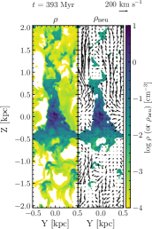
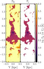
Figure 22.— Density and temperature slices for a snapshot of a fiducial TIGRESS model at $t=393$ Myr. From the first to the fourth panel are shown the total hydrogen density ($\rho$), neutral hydrogen density ($\rho_{{\rm neu}}$), kinetic temperature ($T_{{\rm K}}$), and spin temperature ($T_{{\rm s}}$), respectively. The velocity field of fluid is also displayed overlaid on the second panel. The velocity scale is shown at the top of the second panel.

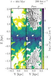
Figure 23.— Density and temperature slices for a snapshot of a fiducial TIGRESS model at $t=464$ Myr. From the first to the fourth panels are shown the total hydrogen density, neutral hydrogen density, kinetic temperature, and spin temperature, respectively. The velocity field of fluid is also displayed overlaid on the second panel. The velocity scale is shown at the top of the second panel.

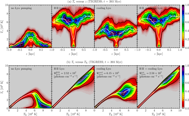
Figure 24.— Spin temperature calculated for a snapshot of a fiducial TIGRESS model at $t=393$ Myr. The top panels show the spin temperature as a function of height and the bottom panels the spin temperature vs the kinetic temperature. From left to right, the panels show the spin temperature (a) when no Ly$\alpha$ pumping is considered, (b) when only Ly$\alpha$ photons originating from H II regions are taken into consideration, (c) when cooling Ly$\alpha$ photons are the only pumping source, and (d) when both Ly$\alpha$ sources are taken into account. The white dots and lines represent the mode and mean of the spin temperature, weighted with the neutral hydrogen density, at each abscissa bin, respectively. The colors represent the 2D cumulative distribution of occurrence of $(z,T_{{\rm s}})$ or $(T_{{\rm K}},T_{{\rm s}})$. The contours denote the locations that discriminate cumulative occurrences of $P_{c}=$ 0.05, 0.3, 0.6, and 0.9; the outermost contour corresponds to $P_{c}=0.05$.

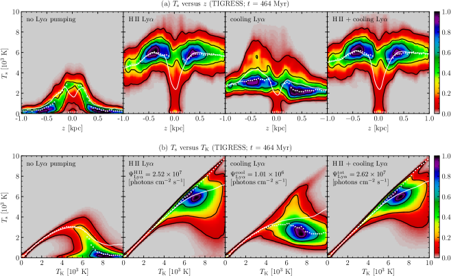
Figure 25.— Spin temperature calculated for a snapshot of a fiducial TIGRESS model at $t=464$ Myr. The top panels show the spin temperature as a function of height and the bottom panels the spin temperature vs the kinetic temperature. From left to right, the panels show the spin temperature (a) when no Ly$\alpha$ pumping is considered, (b) when only Ly$\alpha$ photons originating from H II regions are taken into consideration, (c) when cooling Ly$\alpha$ photons are the only pumping source, and (d) when both Ly$\alpha$ sources are taken into account. The white dots and lines represent the mode and mean of the spin temperature, weighted with the neutral hydrogen density, at each abscissa bin, respectively. The colors and contours show the 2D cumulative frequency of occurrence, as in Figure (24). The contours denote the locations that discriminate cumulative occurrences of $P_{c}=$ 0.05, 0.3, 0.6, and 0.9.

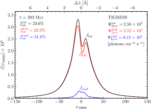
Figure 26.— The emergent spectra obtained from the same snapshot (at $t=363$ Myr) as that used in Figure 24. The red and blue lines show the Ly$\alpha$ spectra originating from H II regions and collisional processes, respectively. The black line represents the total Ly$\alpha$ spectrum. The escape fraction and production rate for each source are also shown.

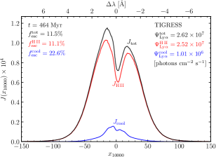
Figure 27.— The emergent spectra calculated for the same snapshot (at $t=464$ Myr) as that used in Figure 25. The red and blue lines show the Ly$\alpha$ spectra originating from H II regions and collisional processes, respectively. The black line represents the total Ly$\alpha$ spectrum. The escape fraction and production rate for each source are also shown.

5.4. The TIGRESS Model

We now use a multiphase ISM model simulated by the Three-phase Interstellar Medium in Galaxies Resolving Evolution with Star Formation and Supernova Feedback (TIGRESS) framework (Kim & Ostriker, 2017) to investigate the spin temperature of the WNM. In the TIGRESS framework, the ideal magnetohydrodynamics equations are solved in a local, shearing box, representing a small patch of a differentially rotating galactic disk. The framework includes self-gravity, star formation (followed by sink particles), and stellar feedback in the forms of FUV photoelectric heating and supernova and yields realistic, fully self-consistent 3D ISM models with self-regulated star formation. The resulting simulation shows realistic gas properties, including mass/volume fractions, turbulence velocities, and scale heights of cold, warm, and hot phases. Furthermore, self-consistently modeled supernova feedback enables to produce inflow/outflow cycles in the extraplanar region via warm fountains and hot winds (Kim & Ostriker, 2018; Vijayan et al., 2019). Both mean and turbulent magnetic fields are generated and saturated through galactic dynamos, reproducing realistic polarized dust emission maps (Kim et al., 2019).

In the present work, we utilize a fiducial ISM model suitable for the solar neighborhood with a uniform spatial resolution of 8 pc. The simulation box size is $L_{x}=L_{y}=1024$ pc and $L_{z}=7168$ pc. The shearing-periodic boundary conditions were applied when photon packets cross the simulation domain horizontally. We subtract a velocity difference due to the galactic differential rotation, $\textbf{v}_{{\rm shear}}=-q\Omega L_{x}\hat{\mathbf{y}}$, when crossing the horizontal boundaries. Here, we adopt a flat rotation curve with the shear parameter $q\equiv\left|d\ln\Omega/d\ln R\right|=1$ and galactic rotational speed $\Omega=28$ km s^-1 kpc^-1. We apply the same methods to inject Ly$\alpha$ photons as explained in Section 5.1. We also assumed that Ly$\alpha$ photons comove with the fluid elements from which they originate. In principle, we can utilize star cluster particles formed and followed in the simulation to inject Ly$\alpha$ photons more self-consistently. Although the current TIGRESS framework does not follow ionizing radiation dynamically, the EUV/FUV radiation field is post-processed using the adaptive ray tracing (Kim et al., 2018) to study ionized gas distribution in the solar neighborhood model (Kado-Fong et al., 2020). We defer more comprehensive investigation using those snapshots in the subsequent papers.

Figures 22 and 23 show the slices of the total hydrogen density, neutral hydrogen density, kinetic temperature, and spin temperature at $X=0$ kpc for two snapshots at $t=393$ Myr and 464 Myr, respectively. The fluid velocity fields are also shown. The spin temperature was obtained by taking into account the Ly$\alpha$-pumping effect due to H II regions and cooling gas. We have analyzed 8 snapshots over one orbit time of evolution ($\sim$ 224 Myr). These two snapshots were chosen to present typical results from the Ly$\alpha$ RT for two distinct conditions realized in the simulation. The snapshot at $t=393$ Myr (Figure 22) shows a breakout of hot-bubble driven by recent supernova explosions, resulting in a large volume filling factor of hot gas near the midplane ($f_{V,\,{\rm hot}}\sim 0.4$) and vertically extended neutral medium with a scale height of $H\sim 500$ pc. In the simulation, star formation activities have been low since then. The neutral medium has fallen back ($H\sim 200$ pc) and filled up most of the volume near the midplane ($f_{V,\,{\rm hot}}\sim 0.1$) at $t=464$ Myr (Figure 23). Consequently, the midplane density of the neutral medium is lower at $t=393$ Myr than at $t=464$ Myr. The snapshot at $t=393$ Myr also has a high-velocity tail in the velocity distribution measured near the midplane and in general higher fluid velocities.

Figures 24 and 25 show the spin temperature calculated for the two snapshots at $t=393$ Myr and 464 Myr, respectively. In the figures, the top panels show the spin temperature as a function of the Galactic altitude, and the bottom panels compare the spin temperature with the gas kinetic temperature. The first to the fourth columns, respectively, show the spin temperature obtained (1) when no Ly$\alpha$ pumping is applied at all, (2) when H II regions are the only Ly$\alpha$ source, (3) when Ly$\alpha$ photons originate only from collisional cooling, and (4) when H II regions and collisional processes are both taken into account.

In the figures, the white dots and curves show the mode and mean of the spin temperature weighted with the density of neutral hydrogen at each abscissa bin, respectively. The colors represent the 2D cumulative distribution of occurrence of a pair $(x,y)=(z,T_{{\rm s}})$ or $(T_{{\rm K}},T_{{\rm s}})$. To build the 2D cumulative distribution, we first constructed a 2D histogram $H_{x,y}$ of the number of volume elements in the 2D space $(x,y)$. The 2D histogram was made to have the number of bins $100\times 100$ and then smoothed with a Gaussian function with $\sigma=1.2$ bins. The 2D cumulative distribution was then obtained by calculating $P_{c}(x,y)=\sum_{i,j}H_{i,j}$, where the summation was performed over the 2D bins $(i,j)$ satisfying $H_{i,j}\leq H_{x,y}$, and by normalizing it with the maximum of $P_{c}(x,y)$. Figures 24 and 25 show the contours that correspond to $P_{c}=$ 0.05, 0.3, 0.6, and 0.9.

As gas density drops at high altitudes, the spin temperature appears to be very low at high altitudes when no Ly$\alpha$ pumping is considered. As shown in the first bottom panels, the spin temperature traces well the kinetic temperature in the low-temperature regime of $T_{{\rm K}}\lesssim 3000-4000$ K, even without Ly$\alpha$ pumping, but traces very poorly at higher temperatures. The spin temperature decreases down to a few hundred Kelvin (even lower than 100 K at some locations) as the kinetic temperature increases ($T_{{\rm K}}\gtrsim 5000$ K). This trend is because the gas density decreases to a too low level to bring the spin temperature to the kinetic temperature with collisional pumping alone as the height increases above $\sim 200$ pc. The result would lead to difficulty in discriminating the thermally stable WNM from the thermally unstable H I gas.

When we include the indirect pumping effect by Ly$\alpha$ photons originating from H II regions, the majority of the WNM is found to have spin temperatures that are very close to the kinetic temperature, as seen in the second bottom panels of Figures 24 and 25. However, a minor fraction of the WNM with $T_{{\rm K}}\gtrsim 6000$ K at high altitudes ($|z|\gtrsim 500$ pc) can still have very low spin temperatures ($T_{{\rm s}}\lesssim 1000$ K) as shown in the snapshot at $t=$ 464 Myr (Figure 25). This result indicates that a substantial portion of Ly$\alpha$ photons is absorbed by dust grains in the galactic plane, and thus not all Ly$\alpha$ photons can reach high altitudes.

As shown in the third columns of Figures 24 and 25, cooling Ly$\alpha$ photons can also pump the spin temperature of the WNM up to a few thousand Kelvin, although not high enough. A substantial fraction of cooling Ly$\alpha$ photons are produced at high altitudes and relatively free from the destruction by dust grains, and thus are fairly efficient in thermalizing the spin temperature of the WNM, although the Ly$\alpha$ production rate is as low as $\sim 2-4$% of that by H II regions.

The last columns of Figures 24 and 25 show the final spin temperature as Ly$\alpha$ photons from both H II regions and collisional cooling gas play roles in raising the spin temperature. The degree of thermalization in Figure 25 is less than perfect compared to the case in Figure 24, which is mainly due to the enhanced dust absorption of the particular snapshot at $t=464$ Myr. Still, in the snapshot at $t=464$ Myr, only a minor fraction of the WNM appears to have more or less low spin temperatures, but not as low as $T_{{\rm s}}\lesssim 1000$ K. In the additional six snapshots we analyzed (not presented here), the thermalization by the WF effect is efficient enough to make the spin temperature as close as the kinetic temperature for the WNM (mostly due to Ly$\alpha$ photons from H II regions, but cooling Ly$\alpha$ photons can maintain $T_{s}>1000$ K at high altitudes).

Figures 26 and 27 present the average Ly$\alpha$ spectra emerging from the top and bottom of the simulation domain for the same snapshots as those for Figures 24 and 25, respectively. In the figures, the emergent Ly$\alpha$ spectra originating from H II regions and cooling gas are shown in red and blue, respectively. The total spectra, including both sources, are shown in black. The escape fractions of Ly$\alpha$ photons are also denoted in the figures. As noted in the case of the Ferriere-ISM model of Section 5.3, the escape fraction of cooling Ly$\alpha$ photons is, in general, higher than that from H II regions. The spectra obtained from both snapshots are asymmetric in the sense that the red part is stronger than the blue part. However, the blue part did not wholly disappear, and it is still strong.

There are three differences between Figures 26 and 27. First, the spectrum emerging from the snapshot of $t=393$ Myr is found to be in general narrower, but have more extended wings, than that from the snapshot at $t=464$ Myr. Second, the escape fraction ($f_{{\rm esc}}^{{\rm Ly}\alpha}=$ 23.6%) from the first snapshot is as more than twofold higher than that ($f_{{\rm esc}}^{{\rm Ly}\alpha}=$ 11.5%) in the second snapshot. Third, the average number of scatterings ($N_{{\rm scatt}}=2.97\times 10^{6}$) in the first snapshot is slightly lower than that ($N_{{\rm scatt}}=3.29\times 10^{6}$) in the second. These differences are mainly due to the difference in the scale height. The snapshots at $t=393$ and 464 Myr is peak and dip in the scale height evolution; therefore, the snapshot at $t=464$ Myr has slightly higher densities, lower temperatures, and slower fluid velocities in the midplane, where most scattering events occur, compared to the snapshot at $t=393$ Myr. These differences are shown in Figures 22 and 23. The effects gave rise to a broader spectrum and stronger absorption of Ly$\alpha$ photons by dust grains for the snapshot at $t=464$ Myr. The extended wings in the spectrum emerging from the snapshot at $t=393$ Myr (Figure 26) are mainly due to a high-velocity tail in the velocity distribution that happened in the midplane of that snapshot. These two snapshots bracket the characteristics shown in the additional six snapshots analyzed (but not shown). The escape fraction was estimated to be in general $f_{{\rm esc}}^{{\rm Ly}\alpha}\approx 7-20\%$.

One other noteworthy aspect is that we had to use at least more than $(2-7)\times 10^{7}$ photon packets, depending on a snapshot, to calculate the scattering rate for the TIGRESS model with a spatial resolution of 8 pc. With only $10^{7}$ or fewer photon packets, the calculated scattering rate was not fully converged, in a statistical sense, at high altitudes, and the resulting spin temperature was found to be underestimated, compared to those obtained with a larger number of photon packets, in a considerable portion of the simulation box. The emergent spectrum and escape fraction converged within $\sim$2% with only $10^{7}$ photons. We used $10^{8}$ photon packets to obtain Figures 24 to 27.

6. DISCUSSION

The WF effect has been extensively studied to use the 21-cm signal to investigate the epoch of reionization (e.g., Furlanetto et al., 2006). In this context, a Monte-Carlo RT method was used in Semelin et al. (2007) and Baek et al. (2009). However, they only counted the number of scatterings of Ly$\alpha$ photons to calculate the 21-cm spin temperature. No Monte-Carlo Ly$\alpha$ RT simulation has been performed, as far as we know, to study the effect of recoil on the slope of the Ly$\alpha$ spectrum or to understand the WF effect in the context of the ISM. The present study provides the most unambiguous results on the necessary condition for the WF effect. In the following, we discuss some topics that are relevant to our results.

6.1. The critical optical depth for the WF effect

Deguchi & Watson (1985) found that a Sobolev optical depth of $\tau_{{\rm LVG}}\approx 10^{5}-10^{6}$ will bring the color temperature to the kinetic temperature. In order to solve the RT equation, they assumed the LVG condition, the so-called Sobolev approximation. The Sobolev optical depth is a measure of the optical thickness of the resonance zone over which the velocity gradient in a moving medium induces a velocity difference ($\Delta V$) equal to the thermal velocity ($v_{{\rm th}}$), along a given ray, as follows:

$$\tau_{{\rm LVG}}\equiv\frac{n_{{\rm H}}\chi_{0}}{(\nu_{\alpha}/c)\left|dV/ds\right|}.$$ (44)

The resonance zone can be regarded as a stationary patch of the medium in the comoving frame. Therefore, the result of Deguchi & Watson (1985) indicates that the minimum optical depth for the WF effect is $\tau_{0}\approx 10^{5}-10^{6}$, which is too large compared to ours. In the LVG method, a resonance line at any location (i.e., resonance zone) in the cloud is assumed to be completely decoupled from resonance at all other locations in the cloud due to point-to-point velocity differences. In other words, photons should not be diffused out more than one Doppler width $\Delta\nu_{{\rm D}}$ in frequency in a local resonance zone. Otherwise, the photons would have opportunities to be absorbed at other locations due to the velocity gradient. The frequency shift due to radiative diffusion in a local resonance zone with an optical depth $\tau_{0}$ is given by $|x|\approx\left(a\tau_{0}\right)^{1/3}$ (Neufeld, 1990). Thus, the condition for the LVG method should be $|x|\lesssim 1$ or $\tau_{{\rm LVG}}\lesssim 1/a=2.12\times 10^{3}(T_{{\rm K}}/10^{4}\,\text{K})^{1/2}$. This condition is not self-consistent with $\tau_{{\rm LVG}}\approx 10^{5}-10^{6}$ and indicates that the LVG method is not adequate for the problem to find the minimum optical depth for the WF effect.

Meiksin (2006) numerically solved the RT equation for resonant photons in various approximate forms to find the time-scale over which the color temperature relaxes to the kinetic temperature of the gas, and obtained results, in some solutions, that the color temperature approaches the kinetic temperature. However, his solutions showed weird oscillatory behaviors near the line center, most likely due to adopted approximations and unstable numerical methods. Roy et al. (2009) made use of a reliable numerical technique to solve the time-dependent RT equation for a homogeneous and isotropically expanding infinite medium. They found that the color temperature of Ly$\alpha$ becomes close to the kinetic temperature after photons have undergone $\sim 10^{4}$ scatterings for $T_{{\rm K}}=10$ K and $\sim 10^{5}$ scatterings for $T_{{\rm K}}=100$ K (see their Figure 4). These critical optical depths are $\sim 10^{2}-10^{3}$ times higher than ours. It is not clear what caused this discrepancy.

Using a Monte-Carlo method, Higgins & Meiksin (2012) calculated the Ly$\alpha$ spectral shape inside the scattering medium to verify their numerical method. However, no Monte-Carlo simulation was performed to investigate the effect of recoil. Instead, they numerically solved the RT equation, including the recoil effect, for an expanding medium with $T_{{\rm K}}=10$ K and mentioned, with regard to their Figure 10, that the expected spectral gradient is recovered across the line center; no detailed analysis, however, was made about the basic requirements for the WF effect.

6.2. Turbulence Effect

In Section 4, we investigated the effect of turbulent motion on the Ly$\alpha$ spectrum within the medium of atomic hydrogen. Spectroscopic observations of many molecular clouds have revealed that the internal velocity dispersion ($v_{{\rm turb}}$, deduced from the line width) of each region is well correlated with its size ($L$) and mass, and these correlations are approximately of power-law form (Larson, 1981; Heyer & Brunt, 2004), as follows:

$$v_{{\rm turb}}=1.10\left(L/\text{pc}\right)^{0.38}\ \text{km}\,\text{s}^{-1}.$$ (45)

The above size-line width dispersion gives the ratio of the internal velocity dispersion to the thermal dispersion of clouds in terms of the optical thickness $\tau_{0}=\left(\chi_{0}/\Delta\nu_{{\rm D}}\sqrt{\pi}\right)n_{{\rm H}}L$ for Ly$\alpha$ photons:

$$\frac{v_{{\rm turb}}}{v_{{\rm th}}}=9\times 10^{-3}\left(\frac{T_{{\rm K}}}{10^{4}\,\text{K}}\right)^{-0.31}\left(\frac{\tau_{0}/500}{n_{{\rm H}}/\text{cm}^{-3}}\right)^{0.38}.$$ (46)

Therefore, in most astrophysical cases, the turbulent velocity dispersion of a cloud with an optical depth of $\tau_{0}\approx 500$ appears to be much smaller than the thermal velocity dispersion. This relation implies that a region corresponding to $\tau_{0}\approx 500$ can be almost always considered to be coherent in velocity. In other words, a coherent zone in which the point-to-point velocity fluctuation is less than the thermal velocity dispersion would have an optical thickness much larger than $\tau_{0}\approx 500$. Thus, turbulent motions in most, if not all, astrophysical circumstances can be regarded as the macroturbulence case concerning the WF effect. This implies that the turbulence motion should not be taken into account in calculating the color temperature of Ly$\alpha$ radiation.

6.3. Ly$\alpha$ Sources and Escape Fraction

In Section 5, we considered two types of Ly$\alpha$ sources: (1) Ly$\alpha$ photons originating from H II regions near the galactic plane and (2) cooling radiation from the ionized gas. In order to calculate the emissivity for the ionized gas, we assumed the CIE condition. Concerning the spatial distribution of H II regions, we assumed a Gaussian distribution in the vertical direction. However, in reality, H II regions would be mostly clustered around the OB associations. The H II regions surrounded by dense neutral gas clouds would then produce L$\alpha$ photons that are eventually absorbed locally by the adjacent clouds. Lallement et al. (2011) used the Voyager measurements to detect Ly$\alpha$ emission from our Galaxy. They estimated the escape fraction of the Ly$\alpha$ radiation from brightest H II regions to be on the order of 3%, but it was highly spatially variable. This effect might strongly suppress the strength of the Ly$\alpha$ radiation from H II regions, and consequently the coupling of Ly$\alpha$ with the 21-cm spin temperature would be less effective than we found in this paper.

However, the WIM, which is known to be produced by the leakage of Lyc photons originating from H II regions to the diffuse, low-density regions (Haffner et al., 2009), could be another important source of Ly$\alpha$ photons. In Figures 24 and 25, it is shown that Ly$\alpha$ radiation from cooling gas under the CIE condition could be an efficient, though not perfect, source to raise the spin temperature of the WNM in the regions where Ly$\alpha$ photons from H II regions could not reach. The luminosity of diffuse H$\alpha$ radiation is known to occupy $\sim 20-50$% of the total H$\alpha$ luminosity in star-forming galaxies. If the diffuse H$\alpha$ radiation originates from the WIM, the same WIM should also produce Ly$\alpha$ photons that are comparable, in amount, with the Ly$\alpha$ photons from H II regions (for an alternative explanation on the origin of the diffuse H$\alpha$, see Witt et al., 2010; Seon & Witt, 2012). This amount is much higher than that estimated to be produced by the cooling gas in the CIE condition. Therefore, Ly$\alpha$ photons originating from the WIM could play a significant role in thermalizing the spin temperature of the WNM. In addition to these sources, cosmic rays can also produce Ly$\alpha$, both by direct excitation by suprathermal secondary electrons and by collisional ionization followed by recombination. As a consequence of all these Ly$\alpha$ sources, we expect that the WF effect would be efficient, at least in the Milky Way-like galaxies.

The escape fraction ($f_{{\rm esc}}^{{\rm Ly}\alpha}$) and spectral shape of the emergent Ly$\alpha$ radiation is highly sensitive to the density structure and kinematic properties of the neutral ISM, including dust. It is, therefore, worthwhile to compare the escape fraction predicted from our models with the observations of external galaxies. Hayes et al. (2011) compiled the observational results from the literature on the escape fraction and derived an average relationship between $f_{{\rm esc}}^{{\rm Ly}\alpha}$ and the color excess $E(B-V)$, i.e., $f_{{\rm esc}}^{{\rm Ly}\alpha}=0.445\times 10^{-5.52E(B-V)}$. However, observational data show a rather large variation in $f_{{\rm esc}}^{{\rm Ly}\alpha}$ for a given $E(B-V)$. $E(B-V)$ for our TIGRESS snapshots is $\approx 0.15$ and it gives $f_{{\rm esc}}^{{\rm Ly}\alpha}\sim 7\%$. Our results ($f_{{\rm esc}}^{{\rm Ly}\alpha}\approx 7-20\%$) are slightly higher than this value, but yet within the variation range observed from external galaxies.

6.4. The Escape Probability Method

Shaw et al. (2017) claimed that the common assumptions that the “excitation” temperature ($T_{{\rm exc}}$) for Ly$\alpha$ transition in hydrogen atoms traces the kinetic temperature ($T_{{\rm K}}$) of gas, and the Ly$\alpha$ radiation drives the 21-cm spin temperature to the kinetic temperature are not valid. It is, therefore, worthwhile to clarify what made their results differ from ours. We first stress that $T_{{\rm exc}}$ is defined by the relative population between the $2p$ and $1s$ states of hydrogen atoms; on the other hand, the “color” temperature ($T_{\alpha}$) of Ly$\alpha$ radiation refers to the slope of Ly$\alpha$ spectrum (or the occupation number density). The excitation temperature becomes the same as the color temperature if the $2p$ state is mainly populated by the Ly$\alpha$ resonance scattering, rather than by the balance between recombination into $2p$ and the radiative (and collisional) decay into $1s$.

In Shaw et al. (2017), Ly$\alpha$ photons were assumed to be produced by recombination following photoionization and cosmic ray ionization or by collisional de-excitation. They adopted “the first-order escape probability” method to derive the level populations of $1\,{}^{2}S_{1/2}$ and $2\,{}^{2}P_{1/2,3/2}^{{\rm o}}$ states by balancing recombination and de-excitation. The Ly$\alpha$ excitation temperature was then determined by the level population between the two states. In the escape probability method, any transfer of photons in space and frequency is ignored (Rybicki, 1984; Hubeny, 2001). Ly$\alpha$ photons either travel zero distance and are immediately re-absorbed (eventually destroyed by dust grains) at the same position or escape the medium altogether in a single flight. In this sense, the escape probability method is also called “the dichotomous model” or “the normalized on-the-spot approximation.” In other words, only the locally-created Ly$\alpha$ photons are taken into account in estimating the level populations and no diffusion in space and frequency due to the RT effect is taken into consideration. They also appear to investigate the effect of Ly$\alpha$ pumping by the attenuated external, stellar radiation field, but no RT of the external continuum photons was considered. The discrepancy between our results and those of Shaw et al. (2017) is primarily because they did not take into account the RT effect.

A (frequency) redistribution function, which gives the probability that an incoming photon of frequency $\nu^{\prime}$ is scattered as an outgoing photon of frequency $\nu$, is, in general, a linear combination of the distribution functions for coherent scattering and complete redistribution in the atom’s frame (Hubeny & Mihalas, 2014). The redistribution functions for coherent scattering and complete redistribution are designated as $R_{{\rm II}}$ and $R_{{\rm III}}$, respectively (Hummer, 1962). The escape probability method is based on the complete redistribution function, which is valid for describing the complete decorrelation (or reshuffling) between the absorbed and re-emitted frequencies in a collision-dominant, high-density medium. The branching ratio between them is given by a ratio of the elastic collision rate to the spontaneous emission rate. The density in the ISM is much lower than the critical density at which the collisional de-excitation rate is equal to the rate of spontaneous radiative decay, as discussed in Dijkstra et al. (2006). The rate at which excited hydrogen atom is perturbed is at most $0.1$ s^-1, even at the electron density of $\sim 10^{2}$ cm^-3, which is nine orders of magnitude below the spontaneous decay rate $\sim 10^{8}$ s^-1. Therefore, the Ly$\alpha$ scattering must be coherent in the atom’s rest frame.

It is known that even for a pure $R_{{\rm II}}$ redistribution function without a contribution of the complete redistribution part, the source function is constant with frequency in the line core for line center optical depths in Ly$\alpha$ larger than about $10^{3}$, as first demonstrated by Hummer (1969). Note that the recoil effect was not included in this $R_{{\rm II}}$ redistribution function. Field (1959b) showed that the Ly$\alpha$ line profile progressively widens and flattens as scattering occurs repeatedly, if no recoil effect of hydrogen atoms were taken into account. The analytical solution of the RT in Neufeld (1990) for a slab also shows flat spectra. Higgins & Meiksin (2012) numerically solved the RT equation in a static sphere using moment equations and showed that the line profile within the medium is indeed flat at the central portion. We also showed that the line profile is indeed a constant when no recoil effect is considered and the optical depth is larger than $\sim 10^{2}$.

The photon loses energy due to recoil in the rest frame of the atom. This effect yields a slope of $-h/k_{{\rm B}}T_{{\rm K}}$ at the central portion of the Ly$\alpha$ profile. Adams (1971) speculated that recoil might not play an important role in the escape of resonance radiation. He claimed that, in the observer’s frame, the small recoil redshift might be almost entirely swamped by the Doppler shifts due to the thermal motion of atoms. He also estimated how many scatterings are needed for recoil to affect the escape of Ly$\alpha$ from a very thick medium. Photons would receive a frequency shift of one Doppler width in each scattering. The recoil shift is about $10^{4}$ times smaller than the Doppler shift at $T_{{\rm K}}=10^{4}$ K, and thus a very large number of scatterings is needed for the recoil effect to significantly shift the photon frequency to the red wing and then boost the escape of Ly$\alpha$ from the medium. He concluded that recoil can be neglected when Ly$\alpha$ undergoes less than $5.6\times 10^{10}$ scatterings. However, the effect of recoil is systematic while the Doppler shift is random. This systematic effect, though it would be tiny, is what shapes the Ly$\alpha$ line profile near the line center, as we demonstrated in Section 4. Shaw et al. (2017) argued that the results of Adams (1971) on the effect of recoil on the Ly$\alpha$ RT support that the recoil effect is not strong enough to bring the spin temperature to the gas kinetic temperature. However, it should be stressed that the study of Adams (1971) is not about the effect of recoil on the Ly$\alpha$ spectral shape within the medium, but mainly on the escape of Ly$\alpha$ from a medium. What matters in the WF effect is a small slope in Ly$\alpha$ profile near the line center, rather than a significantly large redshift of the Ly$\alpha$ frequency to the red wing.

7. SUMMARY

In this paper, we have studied the Ly$\alpha$ RT and WF effect in detail using a Monte-Carlo RT code, named LaRT. LaRT is capable of dealing with not only the WF effect but also the effects due to the fine-structure splitting. LaRT has been successfully used to model the Ly$\alpha$ spectra and surface brightness profiles of the Ly$\alpha$ emitting galaxies at $z=3-6$ (Song et al. 2019, submitted to ApJ). The main aim of the present study was to investigate the WF effect on the spin temperature of the WNM. However, most of our results are applicable in the context of the CGM and IGM. The numerical results of the models will be made available to the community via the authors’ WWW site . Our calculations were performed using an unprecedentedly large number of photon packets and thus will be useful for benchmark tests. The principal conclusions of this paper are as follows:

1. As a result of the recoil effect, the color temperature of the Ly$\alpha$ line profile approaches the gas kinetic temperature even in a medium with as low as $\tau_{0}\approx 100-500$, which is much lower than those predicted in previous studies.

2. Even in an expanding or turbulent medium, the Ly$\alpha$ spectrum within the medium is fully thermalized to have a color temperature equal to the kinetic temperature due to recoil of hydrogen atom, unless the optical thickness of a coherent region, over which the flow velocity and kinetic temperature can be regarded to be nearly constant, is less than $\approx 100-500$.

3. We demonstrated that the turbulent motion widens the emergent spectra. However, we showed that the turbulent motion in most astrophysical systems does not change the color temperature of the Ly$\alpha$ spectrum. In other words, the color temperature of Ly$\alpha$ is equal to the gas kinetic temperature even in a turbulent medium.

4. To bring the spin temperature to the kinetic temperature, the Ly$\alpha$ radiation field should also be strong enough. Dust grains may suppress the strength of Ly$\alpha$ radiation by absorbing them. How Ly$\alpha$ photons are effectively destroyed or survive in dusty clouds would strongly depend on the density distribution and kinematic properties of the clouds.

5. Utilizing the ISM model of Ferriere (1998) and a MHD simulation using the TIGRESS framework of Kim & Ostriker (2018), we calculated the spin temperature of the WNM in the vicinity of the Sun and found that the resulting spin temperature is reasonably close to the kinetic temperature in the majority of the ISM. In the Ly$\alpha$ simulations, we included both H II regions and the collisionally cooling gas as Ly$\alpha$ sources.

6. We found that Ly$\alpha$ photons originating from sources in relatively dust-free, high altitude regions, such as the collisionally cooling gas, can play a significant role in regions where Lyα photons from H II regions cannot reach due to suppression by dust grains.

7. In addition to the above main results, we developed a new, efficient algorithm to produce the velocity component of scattering atoms that is parallel to the photon propagation direction, as presented in Appendix 28.

8. We calculated the average number of scatterings in an infinite slab and a sphere for a wide range of optical depths from $\tau_{0}=1$ to $10^{9}$ and two temperatures of $T_{{\rm K}}=10$ K and $10^{4}$ K. We also derived a new analytic formula for the average number of scatterings in a spherical medium. New analytic equations for the scattering rate $P_{\alpha}$ and Ly$\alpha$ line profile in a sphere and slab are also provided. These formulae, as shown in Appendixes B and C, well reproduce the Monte-Carlo simulation results at the limit of large optical depth.

Appendix A The Parallel Velocity of Scattering Atom

Figure 28.— Two-dimensional space $\mathcal{S}$ from which the distribution for the parallel velocity component $u$ of scattering atoms is required to be generated: (a) $F(\beta,\gamma)d\beta d\gamma=f_{0}(\gamma/\beta)d\beta d\gamma$ or (b) $\bar{F}(\beta,u)d\beta du=f_{0}(u)\beta d\beta du$

The probability distribution function for the velocity component $u$ of a scattering atom parallel to the incoming photon is

$$f(u)=\frac{a}{\pi H(x,a)}\frac{e^{-u^{2}}}{(u-x)^{2}+a^{2}},$$ (A1)

which is not analytically integrable. In order to generate random numbers that follow the above distribution, the acceptance/rejection method of Zheng & Miralda-Escudé (2002a) usually has been used. However, we found that the algorithm is fairly inefficient, especially when $x$ is large, and $T_{{\rm K}}$ is high ($a$ is small).

Here, we introduce a new algorithm inspired by the ratio-of-uniforms method (Kinderman & Monahan, 1977). Since the distribution function $f(u)$ is symmetric under the transformation of $(x,u)\leftrightarrow(-x,-u)$, the following discussion is limited to $x>0$.

Suppose that a bivariate random variable $(\beta,\gamma)$ is uniformly distributed while satisfying the following inequality:

$$0\leq\beta\leq\sqrt{f(\gamma/\beta)},$$ (A2)

for any nonnegative function $f(u)$. It can then be proven that $u=\gamma/\beta$ follows a probability density function proportional to $f(u)$. This theorem can be generalized for a product of two distribution functions. If $f(u)=f_{0}(u)f_{1}(u)$ and $(\beta,\gamma)$ has a probability density proportional to $f_{0}(\gamma/\beta)$ over the region of the plane defined by

$$\mathcal{S}=\{(\beta,\gamma):0\leq\beta\leq\sqrt{f_{1}(\gamma/\beta)}\},$$ (A3)

then $u=\gamma/\beta$ follows a density distribution proportional to $f(u)$.

Figure 29.— Schematic shape of $Q(\beta)$ for the case of (a) $x<x_{c}\ (=1+\sqrt{2})$ and (b) $x>x_{c}$. The three domains are denoted by $S_{0}$, $S_{1}$ and $S_{2}$, respectively. Note that the figure is not in scale and the height $h_{2}$ is not always higher than $h_{0}$. In (b), the two areas $S_{0}$ and $S_{1}$ become negligible and $\beta_{0},\,\beta_{1}\ll 1$ when $h_{2}>2h_{0}$. The solid line represents the function $Q(\beta)$ defined in Equation (A8) and the shaded areas are the piecewise comparison function in Equation (A20).

Let us define two functions to apply the above theorem to our problem:

$$f_{0}(u)=\frac{1}{\pi}\frac{1}{(u-x)^{2}+a^{2}}\ \ {\rm and}\ \ f_{1}(u)=e^{-u^{2}}.$$ (A4)

The region $\mathcal{S}$ where $f_{0}(u)$ is defined is equivalent to the following condition:

$$\left|\gamma\right|\leq\beta\sqrt{-2\ln\beta}\ \ {\rm or}\ \ \left|u\right|\leq\sqrt{-2\ln\beta},$$ (A5)

which is illustrated in Figure 28. In other words, the following 2D distribution of $(\beta,\gamma)$ or $(\beta,u)$ should be generated over the area defined by Equation (A5):

$$F(\beta,\gamma)d\beta d\gamma \equiv f_{0}(\gamma/\beta)d\beta d\gamma,$$ (A6)

or

$$\bar{F}(\beta,u)d\beta du \equiv f_{0}(u)\beta d\beta du.$$ (A7)

For our purpose, it is more convenient to deal with two variables $(\beta,u)$ instead of $(\beta,\gamma)$.

To make bivariate random variables $(\beta,u)$ according to $\bar{F}(\beta,\gamma)$, defined over the light-blue region defined in Figure 28(b), we consider the following one-dimensional marginal distribution of $\beta$:

$$Q(\beta) \equiv \int_{-p(\beta)}^{p(\beta)}\bar{F}(\beta,u)du$$ (A8)

$$= \frac{\beta}{a\pi}\left[\tan^{-1}\left(\frac{p(\beta)-x}{a}\right)+\tan^{-1}\left(\frac{p(\beta)+x}{a}\right)\right],$$

where

$$p(\beta)\equiv\sqrt{-2\ln\beta}.$$ (A9)

A bivariate random variable $(\beta,u)$ can be obtained by selecting a random number $\beta$ from the distribution function $Q(\beta)$ and then generating $u$ from $f_{0}(u)$ over the range of $\left|u\right|\leq p(\beta)$. The distribution function $f_{0}(u)$ is analytically invertible, and thus a random number $u$ can be easily obtained for the given random variate $\beta$. The question that is then raised is how to generate random numbers that follow the density distribution $Q(\beta)$.

We generate the random numbers for $Q(\beta)$ using an acceptance/rejection method. To use the technique, we need to construct a comparison function $C(\beta)$ that is similar to, but always higher than, $Q(\beta)$. The overall shape of $Q(\beta)$ is shown in Figure 29. We first decompose $Q(\beta)$ into two domains: $p(\beta)>x$ and $p(\beta)<x$. Let us define $\beta_{0}$, which divides the domains, as follows:

$$\beta_{0}\equiv e^{-x^{2}/2}.$$ (A10)

For the first domain ($S_{0}$; $\beta<\beta_{0}$, $p(\beta)>x$ in Figure 29), we observe that

$$Q(\beta)<\int_{-\infty}^{\infty}\bar{F}(\beta,u)du=\frac{\beta}{a}.$$ (A11)

Here, the last term is a linear function with a slope $1/a$. For the second domain ($S_{1}+S_{2}$; $\beta>\beta_{0}$, $p(\beta)<x$ in Figure 29), we find the following inequality, since $1/\left[(u-x)^{2}+a^{2}\right]<1/(u-x)^{2}$:

$$Q(\beta) < Q^{*}(\beta)\equiv\frac{\beta}{\pi}\int_{-p(\beta)}^{p(\beta)}\frac{du}{(u-x)^{2}}$$ (A12)

$$\ \ \ \ \ \ \ \ \ \ \ =\frac{2\beta}{\pi}\frac{p(\beta)}{x^{2}-p^{2}(\beta)}.$$

We note that $Q^{*}(\beta)$ is very close to $Q(\beta)$ in the range of $\beta>\beta_{1}$ (minimum point in Figure 29(b)), but rapidly diverges to infinity as $\beta\rightarrow\beta_{0}$. These inequalities are summarized as follows:

$$Q(\beta) < \begin{cases}\beta/a&{\rm for}\ \beta<\beta_{0},\ \ \ p(\beta)>x,\\ \\ Q^{*}(\beta)&{\rm for}\ \beta>\beta_{0},\ \ \ p(\beta)<x.\end{cases}$$ (A13)

A notable point is that $Q(\beta)$ has a right triangular shape in the first domain ($\beta<\beta_{0}$), as shown in Figure 29. In the second domain ($\beta>\beta_{0}$), $Q(\beta)$ appears to be more complex. If $x<x_{c}\equiv 1+\sqrt{2}$, $Q(\beta)$ is a monotonically decreasing function of $\beta>\beta_{0}$, as shown in Figure 29(a). On the other hand, if $x>x_{c}$, $Q(\beta)$ shows a minimum and maximum in the domain $S_{1}+S_{2}$. The existence condition of the minimum ($\beta=\beta_{1}$ in Figure 29(b)) and maximum ($\beta=\beta_{2}$) points in the second domain can be easily derived from $dQ^{*}/d\beta=0$; the resulting condition is that $x>x_{c}=1+\sqrt{2}$.

For the efficiency in applying the rejection/acceptance method, we further divide the second domain into two subdomains, as denoted by $S_{1}$ and $S_{2}$ in Figure 29. The basic idea for our comparison function is shown in Figure 29: a triangle for $S_{0}$ and two rectangles for $S_{1}$ and $S_{2}$. In the case of $x<x_{c}$, the location $\beta=\beta_{1}$, where $S_{1}$ and $S_{2}$ are divided, is obtained by minimizing the area $S_{1}+S_{2}=(\beta_{1}-\beta_{0})h_{0}+(1-\beta_{1})h_{1}$. Here, $h_{0}$, the half of the height of the right triangle in $S_{0}$, and $h_{1}$ are given by, respectively,

$$h_{0} \equiv \frac{\beta_{0}}{2a}\geq Q(\beta_{0})=\frac{\beta_{0}}{a\pi}\tan^{-1}\left(\frac{2x}{a}\right),$$ (A14)

$$h_{1} \equiv Q^{*}(\beta_{1}).$$ (A15)

After expanding $d(S_{1}+S_{2})/d\beta$ in a power series of $\beta-\beta_{0}$ and $a$, and setting the derivative to be zero, we obtain

$$\beta_{1}\equiv\beta_{0}+\left[\frac{2a}{\pi}\left(1-\beta_{0}\right)\beta_{0}x\right]^{1/2}.$$ (A16)

We found that this is also a good choice even for $x>x_{c}$; however, this $\beta_{1}$ is not the minimum point in $S_{1}+S_{2}$.

In Figure 29(b) ($x>x_{c}$), the height $h_{2}$ that tightly constrains the true height of $S_{2}$ is obtained to be

$$h_{2} \equiv \frac{2e^{-1/2}p(e^{-1/2})}{\pi}\frac{1}{x^{2}-1.373}=\frac{0.3861}{x^{2}-1.373}.$$ (A17)

This was found by noticing that $\beta=e^{-1/2}$ yields the maximum of $Q^{*}(\beta)$ at the limit of $x\rightarrow\infty$ ($Q(\beta)=Q^{*}(\beta)\rightarrow 2\beta p(\beta)/\pi x^{2}$). However, $Q^{*}(\beta=e^{-1/2})$ was slightly lower than the true maximum of $Q(\beta)$. We, therefore, attempted to find a suitable height $h_{2}$ that tightly constrains the maximum of $Q(\beta)$. In the end, $h_{2}$ in Equation (A17) was obtained by adjusting $p(\beta=e^{-1/2})=1$ in the denominator of $Q^{*}(\beta=e^{-1/2})$ to 1.373. This $h_{2}$ provides a very tight constraint on the maximum of $Q(\beta)$ for any $x$.

Figure 30.— The regions in the $(T_{{\rm K}},x)$ space where we define the three different comparison functions in Equations (A18)-(A20).

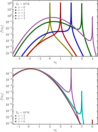
Figure 31.— The distribution of parallel velocities $f(u_{\parallel})$ for different values of incoming frequency $x$. The black curves denote the histograms for the random numbers generated using the present algorithm. The colored curves show the theoretical distribution functions, as calculated from Equation (A1).

Let us now define our comparison function. It is more convenient to combine two or three domains and define a simpler comparison function depending on $h_{2}$. If $h_{2}>2h_{0}$, the areas $S_{0}$ and $S_{1}$ are negligible and we thus combine the three domains as a single domain $S_{0}+S_{1}+S_{2}$. In this case, we choose a single comparison function for the whole domain, as follows:

$$C(\beta)\equiv h_{2}.$$ (A18)

If $h_{0}<h_{2}<2h_{0}$, we combine $S_{1}$ and $S_{2}$ and consider two domains $S_{0}$ and $S_{1}+S_{2}$. This leads us to define the following comparison function:

$$C(\beta)\equiv\begin{cases}\beta/a&{\rm if}\ \ \beta\leq\beta_{0},\\ \\ h_{2}&\text{otherwise},\end{cases}$$ (A19)

The areas of the first and second domains are $S_{0}=\beta_{0}h_{0}$ and $S_{1}=(1-\beta_{0})h_{2}$, respectively. The total area of the comparison function is $S_{{\rm tot}}=S_{0}+S_{1}$.

If $h_{2}<h_{0}$ or $x<x_{c}$, we define the comparison function to be

$$C(\beta)\equiv\begin{cases}\beta/a&{\rm if}\ \ \beta\leq\beta_{0},\\ \\ h_{0}&{\rm if}\ \ \beta_{0}<\beta\leq\beta_{1},\\ \\ h_{1}&{\rm if}\ \ \beta>\beta_{1}\ \ \ {\rm and}\ \ \ x\leq x_{c}.\\ \\ \max(h_{1},h_{2})&{\rm if}\ \ \beta>\beta_{1}\ \ \ {\rm and}\ \ \ x>x_{c}.\end{cases}$$ (A20)

In this case, the areas of the first and second domains are $S_{0}=\beta_{0}h_{0}$ and $S_{1}=(\beta_{1}-\beta_{0})h_{0}$, respectively. The area of the third domain is given by $S_{2}=(1-\beta_{1})h_{1}$ if $x<x_{c}$ or $S_{2}=(1-\beta_{0})\max(h_{1},h_{2})$ if $x>x_{c}$. The total area of the comparison function is $S_{{\rm tot}}=S_{0}+S_{1}+S_{2}$.

We note that the comparison function in $S_{0}$ is a linear function. A random variate for the linear part of the comparison function is obtained using the inversion method; $\beta=\beta_{0}\xi^{1/2}$ for a uniform random number $\xi$.

Supposing that $\xi_{1},\xi_{2},\cdots$ are mutually-independent, uniform random numbers between 0 and 1, our algorithm is given as follows:

1. If $h_{2}\geq 2h_{0}$, we choose $\beta$ as follows:

   $$\beta = \xi_{1}.$$ (A21)

   If $h_{0}\leq h_{2}<2h_{0}$, $\beta$ is obtained by:

   $$\beta=\begin{cases}\beta_{0}\sqrt{\xi_{2}}&{\rm if}\ \ \xi_{1}\leq S_{0}/S_{{\rm tot}},\\ \\ \beta_{0}+\left(1-\beta_{0}\right)\xi_{3}&\text{otherwise}.\end{cases}$$ (A22)

   If $h_{2}<h_{0}$ or $x<x_{c}$, $\beta$ is given by

   $$\beta=\begin{cases}\beta_{0}\sqrt{\xi_{2}}&{\rm if}\ \ \xi_{1}\leq S_{0}/S_{{\rm tot}},\\ \\ \beta_{0}+\left(\beta_{1}-\beta_{0}\right)\xi_{3}&{\rm if}\ \ S_{0}/S_{{\rm tot}}<\xi_{1}\leq 1-S_{2}/S_{{\rm tot}},\\ \\ \beta_{1}+\left(1-\beta_{1}\right)\xi_{4}&\text{otherwise}.\end{cases}$$ (A23)

2. If $\xi_{6}\leq Q(\beta)/C(\beta)$, we accept $\beta$. Otherwise, go back to step 1 and repeat the procedure until $\beta$ is accepted.

3. For the accepted $\beta$, the parallel velocity component $u$ is readily obtained by solving the following equation about $u$:

   $$\int_{-p(\beta)}^{u}\bar{F}(\beta,u^{\prime})du^{\prime}=Q(\beta)\xi_{5}.$$ (A24)

   This gives the following result:

   $$u=x+a\tan\left[\left(\frac{a\pi}{\beta}\right)Q(\beta)\xi_{7}-\tan^{-1}\left(\frac{p(\beta)+x}{a}\right)\right].$$ (A25)

If the input $x$ was negative, we take the negative of $u$ that is obtained after replacing $x$ with its absolute value.

We note that $h_{2}$ is a function of $x$, and $h_{0}$ is a function of $x$ and $a$ (or $T_{{\rm K}}$). Figure 30 shows the regions in the $(T_{{\rm K}},x)$ space where the three different comparison functions in Equations (A18)-(A20) are defined. Figure 31 compares the distribution of random numbers generated using the algorithm developed in this paper with the theoretical probability distribution function Equation (A1). As shown in the figure, our algorithm reproduces the probability distribution function for the parallel velocity component very well.

Our method seems not to be intuitive to understand at first glance. However, the present algorithm is uniformly efficient for any $x$ and $a$. One may use our algorithm only in the cases of $h_{2}>2h_{0}$ and $h_{0}<h_{2}<2h_{0}$ while adopting the method of Zheng & Miralda-Escudé (2002b) in the case of $h_{2}<h_{0}$. We use the algorithm of Zheng & Miralda-Escudé (2002b) for $x<1$ (after setting $u_{0}=0$), and the present algorithm otherwise.

Appendix B Analytic Solutions for a Static, Uniform Slab

Neufeld (1990) derived an approximate series expression for the mean intensity at any point in an infinite slab:

$$J(x,\tau) = F\left(\frac{\tau^{\prime}-\tau^{\prime}_{s}}{2\tau_{0}},\frac{\left|\sigma-\sigma_{i}\right|}{2\tau_{0}}\right),$$ (B1)

$$-F\left(\frac{2\tau_{0}-\tau^{\prime}-\tau^{\prime}_{s}}{2\tau_{0}},\frac{\left|\sigma-\sigma_{i}\right|}{2\tau_{0}}\right)$$

where

$$F(w,y) \equiv \frac{\sqrt{6}}{8\pi}\sum_{n=1}^{\infty}\left[\frac{\cos(n\pi w)e^{-n\pi y}}{n\pi}\right],$$ (B2)

$$\tau^{\prime} \equiv \tau\left(1-\frac{2}{3\phi(x)\sqrt{\pi}\tau_{0}}\right)\simeq\tau\left(1-\frac{2x^{2}}{3a\tau_{0}}\right),$$

$$\sigma \equiv \left(\frac{2\pi}{3}\right)^{1/2}\frac{x^{3}}{3a},$$

$$\phi(x) \equiv \frac{1}{\sqrt{\pi}}H(x,a)\simeq\frac{a}{\pi x^{2}}.$$

Here, the optical depth at the location of the point source is denoted by $\tau_{s}$ and the initial frequency $x_{i}$ is represented by $\sigma_{i}=(2\pi/3)^{1/2}x_{i}^{3}/(3a)$. Note that Neufeld (1990) defines the optical depth as the total optical depth integrated over frequency, i.e., $\tau^{{\rm Neufeld}}=\sqrt{\pi}\tau$ and $\sigma^{{\rm Neufeld}}=\sqrt{\pi}\sigma$. We can further simplify $F(w,y)$ as

$$F(w,y)=-\frac{\sqrt{6}}{16\pi^{2}}\ln\left(1-2e^{-\pi y}\cos\pi w+e^{-2\pi y}\right).$$ (B3)

This is obtained by applying the identity $\cos x=\left(e^{ix}+e^{-ix}\right)/2$, and then simplifying the summation with $\ln\left(1-x\right)=-\sum_{n=1}^{\infty}x^{n}/n$ and $\cosh x=\left(e^{x}+e^{-x}\right)/2$. The mean intensity in the slab can then be written as

$$J(x,\tau)=\frac{\sqrt{6}}{16\pi^{2}}\ln\left[\frac{\cosh\left(\pi\frac{\left|\sigma-\sigma_{i}\right|}{2\tau}\right)+\cos\left(\pi\frac{\tau^{\prime}+\tau_{s}^{\prime}}{2\tau_{0}}\right)}{\cosh\left(\pi\frac{\left|\sigma-\sigma_{i}\right|}{2\tau_{0}}\right)-\cos\left(\pi\frac{\tau^{\prime}-\tau_{s}^{\prime}}{2\tau_{0}}\right)}\right].$$ (B4)

Setting $\tau_{s}=0$ and $x_{i}=\sigma_{i}=0$, the mean intensity becomes:

$$J(x,\tau)=\frac{\sqrt{6}}{16\pi^{2}}\ln\left[\frac{\cosh(\pi\left|\sigma\right|/2\tau_{0})+\cos(\pi\tau^{\prime}/2\tau_{0})}{\cosh(\pi\left|\sigma\right|/2\tau_{0})-\cos(\pi\tau^{\prime}/2\tau_{0})}\right].$$ (B5)

This equation evaluated at $\tau=\tau_{0}$ seems to be different from Equation (2.24) of Neufeld (1990) but gives almost the same numerical results.

The mean intensity at $x=0$ (i.e., $y=\sigma=0$ and $\tau^{\prime}=\tau$) is then given by

$$J_{x}(0,\tau) = -\frac{\sqrt{6}}{8\pi^{2}}\ln\left[\tan\left(\frac{\pi}{4}\frac{\tau}{\tau_{0}}\right)\right]$$

$$\simeq \begin{cases}-\frac{\sqrt{6}}{8\pi^{2}}\ln\left(\frac{\pi}{4}\frac{\tau}{\tau_{0}}\right)&{\rm for}\ \ \tau/\tau_{0}\ll 1\\ \\ \frac{\sqrt{6}}{16\pi}\left(1-\frac{\tau}{\tau_{0}}\right)&{\rm for}\ \ \tau/\tau_{0}\approx 1.\end{cases}$$

As is explained in Section 4, we can use $J_{x}(0,\tau)$ to calculate the scattering rate $P_{\alpha}$ (see Equation (27)).

The average number of scatterings that a photon undergoes before escaping the medium is an integral of the scattering rate over total number of atoms in the whole volume:

$$\left\langle N_{{\rm scatt}}\right\rangle = \int P_{\alpha}n_{{\rm H}}dz$$

$$\simeq 4\pi\int_{-L}^{L}\int_{0}^{\infty}J_{\nu}(0,z)\sigma_{\nu}n_{{\rm H}}d\nu dz,$$

where $n_{{\rm H}}$ is the number density of neutral hydrogen atom. Using Equation (B), we can derive the average number of scatterings to be

$$\left\langle N_{{\rm scatt}}\right\rangle=\left(\frac{4\sqrt{6\pi}C}{\pi^{2}}\right)\tau_{0}=1.612\tau_{0},$$ (B8)

where $C\equiv\sum_{k=0}^{\infty}(-1)^{k}(2k+1)^{-2}\simeq 0.915966$ is Catalan’s constant. Harrington (1973) also obtained the same result by integrating a series solution. The number of scatterings in a slab geometry was also discussed in Adams (1972).

Appendix C Analytic Solution for a Static, Uniform Sphere

Dijkstra et al. (2006) provide a series solution to the RT equation for a uniform sphere, in which photons are emitted at radius $r_{s}$, assuming the Eddington approximation:

$$J(x,r)=\frac{\sqrt{6}}{16\pi^{2}R^{2}}\sum_{n=1}^{\infty}\frac{\sin\left(\lambda_{n}r_{s}\right)\sin\left(\lambda_{n}r\right)}{\left(\lambda_{n}r_{s}\right)\left(r/R\right)}e^{-\lambda_{n}\left|\sigma\right|/\kappa_{0}},$$ (C1)

where

$$\lambda_{n} \equiv \frac{n\pi}{R}\left(1-\frac{1}{1+(3/2)\phi(x)\sqrt{\pi}\tau_{0}}\right),$$

$$\sigma \equiv \left(\frac{2\pi}{3}\right)^{1/2}\frac{x^{3}}{3a}$$

$$\phi(x) \equiv\frac{1}{\sqrt{\pi}} H(x,a)\simeq\frac{a}{\pi x^{2}}.$$

However, the series solution is not practical for an application. They, therefore, derived an analytic formula for the Ly$\alpha$ spectrum emerging from the sphere by setting $r=R$ and simplifying the series solution. In the present study, we need a more general formula for the spectrum of radiation field within the medium at an arbitrary radius. We found that, using the identities $\sin x=\left(e^{ix}-e^{-ix}\right)/2i$, $\ln\left(1-x\right)=-\sum_{n=1}^{\infty}x^{n}/n$, $\cos x=\left(e^{ix}+e^{-ix}\right)/2$, and $\cosh x=\left(e^{x}+e^{-x}\right)/2$, the series solution of $J(x,r)$ can be rewritten as

$$J(x,r) = \frac{1}{4\pi R^{2}}\frac{\sqrt{6}}{16\pi}\frac{1}{q(r_{s}/R)(r/R)}$$ (C2)

$$\times\ln\left[\frac{\cosh\left(q\left|\sigma\right|/\tau_{0}\right)-\cos\left(q(r+r_{s})/R\right)}{\cosh\left(q\left|\sigma\right|/\tau_{0}\right)-\cos\left(q(r-r_{s})/R\right)}\right],$$

where

$$q\equiv\lambda_{1}R\simeq\pi\left(1-\frac{2\sqrt{\pi}x^{2}}{3a\tau_{0}}\right).$$

However, the above equation has a singularity at the first term as $r_{s}\rightarrow 0$. For the case of $r_{s}=0$, we use the asymptotic property $\sin(x)/x\rightarrow 1$ as $x\rightarrow 0$ in the series solution (Equation (C1)) and find an analytic solution to be

$$J(x,r) = \frac{1}{4\pi R^{2}}\frac{\sqrt{6}}{8\pi}$$ (C3)

$$\times\left(\frac{R}{r}\right)\frac{\sin\left(qr/R\right)}{\cosh\left(q\left|\sigma\right|/\tau_{0}\right)-\cos\left(qr/R\right)}.$$

At the limit of $r=R$ and $\tau_{0}\rightarrow\infty$, this equation becomes the same as Equation (C17) of Dijkstra et al. (2006). From the equation, the mean intensity at $x=0$ is obtained to be

$$J_{x}(0,r) = \frac{1}{4\pi R^{2}}\frac{\sqrt{6}}{8\pi}\left(\frac{R}{r}\right)\cot\left(\frac{\pi}{2}\frac{r}{R}\right)$$

$$\simeq \begin{cases}\frac{1}{4\pi R^{2}}\frac{\sqrt{6}}{4\pi^{2}}\left(\frac{R}{r}\right)^{2}&{\rm for}\ \ r/R\ll 1\\ \\ \frac{1}{4\pi R^{2}}\frac{\sqrt{6}}{16}\left(\frac{R}{r}\right)\left(1-\frac{r}{R}\right)&{\rm for}\ \ r/R\approx 1,\end{cases}$$

which can be used to estimate the scattering rate $P_{\alpha}$ (see Equation (27)). Interestingly, the solution indicates the free streaming radiation in the vicinity of the source ($r/R\ll 1$). As in Appendix B, the number of scatterings is the number of scattering events per unit time over the whole medium divided by the generation rate. We derive the average number of scatterings that a photon undergoes before escaping the sphere to be

$$\left\langle N_{{\rm scatt}}\right\rangle = 4\pi\int_{0}^{R}P_{\alpha}n_{{\rm H}}4\pi r^{2}dr$$ (C5)

$$\simeq 4\pi\int_{0}^{R}\int_{0}^{\infty}J_{\nu}(0,r)n_{{\rm H}}\sigma_{\nu}4\pi r^{2}d\nu dr$$

$$= \left(\sqrt{\frac{3}{2\pi}}\ln 4\right)\tau_{0}=0.9579\tau_{0}.$$

This is the solution at the limit of $\tau_{0}\rightarrow\infty$. We also note that the analytic solutions for the mean intensity and scattering rate in an expanding medium with zero temperature were derived in Loeb & Rybicki (1999) and Higgins & Meiksin (2012).

Appendix D Dust-Absorbed Ly$\alpha$ Spectrum

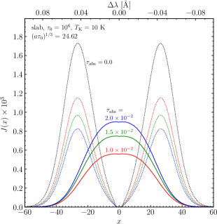
Figure 32.— Emergent and dust-absorbed Ly$\alpha$ spectra for an infinite slab geometry with a temperature of $T_{{\rm K}}=10^{4}$ K and the H I optical depth of $\tau_{0}=10^{6}$. The black dotted line represents the emergent Ly$\alpha$ spectrum when no dust is included. The red, green, and blue curves denote the cases for the dust absorption optical depths of $\tau_{{\rm abs}}=1.0\times 10^{-2}$, $1.5\times 10^{-2}$, and $2.0\times 10^{-2}$, respectively. The solid and dotted lines indicate the emergent and absorbed spectra, respectively.

To understand the origin of the dip feature in the dust-absorbed Ly$\alpha$ spectra, as shown in Figure 5, we need to consider two competing factors, as pointed out in Verhamme et al. (2006): (1) a relatively, very low probability of being absorbed by dust grains compared to that of the strong H I scattering at the line center ($x=0$), and (2) a large number of resonance scatterings that photons undergo in the line core, increasing the opportunity of interacting with dust in the end. The ratio of dust extinction to the H I scattering cross-section is proportional to $T_{{\rm K}}^{1/2}$ at the Ly$\alpha$ line center, and thus the relative likelihood of photons to be absorbed by dust grains decreases as temperature decreases. This implies that the first factor is more important at lower temperatures. It can also be readily understood that the first effect would be more important at lower optical depths. As the optical depth increases, the increased number of interactions compensates the inefficiency of dust absorption at the line center and makes the second factor important. Even a slight increase of $\tau_{{\rm abs}}$ could yield a much stronger absorption; the dip feature would then disappear as $\tau_{{\rm abs}}$ increases, as shown in Figure 32.

Figure 32 shows some spectra resulting from attempts to reproduce Figure 3 of Verhamme et al. (2006). The three models in Figure 32 were selected to be reasonably close to their model. We note that Figure 32 assumes much higher dust-absorption optical depths than in Figure 5. In Figure 32, we found no clear dip feature in the absorbed spectra, expect a minor sign of deviation from the perfect flatness at $x=0$, as opposed to Figure 3 of Verhamme et al. (2006). The cause of the discrepancy is not clear. We also found that the dip feature slightly changes as a less accurate Voigt profile function, for instance, used in Tasitsiomi (2006) and Laursen et al. (2009), is adopted.

Appendix E Physics of the WF Effect

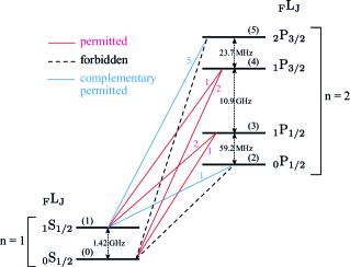
Figure 33.— The hyperfine energy levels ($n=1$ and $n=2$) of hydrogen. The energy levels are designated by ${}_{F}L_{J}$ and labeled in parentheses. The solid red and dashed black lines denote permitted and forbidden transitions, respectively. The solid blue lines are also permitted transitions, but complementary in the sense that they are not relevant to exciting the 21-cm line. The relative line strengths ($S_{51}:S_{41}:S_{40}:S_{31}:S_{30}:S_{21}=5:1:2:2:1:1$) of the six permitted transitions are also denoted. Frequencies between the hyperfine states are also shown.

In the context of the ISM research, the WF effect has not been fully described. It is, therefore, worthwhile to summarize the fundamental physics of the WF effect to clarify the necessary conditions to fulfill the WF effect. Figure 33 shows the energy level diagram for the hyperfine structure of hydrogen. There are three kinds of excitation (or de-excitation) mechanisms that determine the relative population between the two hyperfine levels of the $1^{2}S_{1/2}$ ground state of hydrogen: collisional transition, radiative transition, and Ly$\alpha$ pumping. In the stationary state, the rate equation for the population of the hyperfine states “0” and “1” can be written as follows:

$$n_{0}\left(P_{01}^{{\rm R}}+P_{01}^{{\rm c}}+P_{01}^{\alpha}\right)=n_{1}\left(P_{10}^{{\rm R}}+P_{10}^{{\rm c}}+P_{10}^{\alpha}\right),$$ (E1)

where $n_{0}$ and $n_{1}$ are populations of the sublevels “0” and “1,” and $P^{{\rm R}}$, $P^{{\rm c}}$, and $P^{\alpha}$ are transition rates (per sec) caused by radiation (21 cm), collisions, and Ly$\alpha$ pumping, respectively. The subscript $ji$ denotes the transition from the sublevel $j$ to $i$. According to the definition of spin temperature ($T_{{\rm s}}$), the relative population between the sublevels “0” and “1” is given by

$$\frac{n_{1}}{n_{0}}=\frac{g_{1}}{g_{0}}\exp\left(-\frac{h\nu_{10}}{k_{{\rm B}}T_{{\rm s}}}\right)\simeq 3\left(1-\frac{T_{*}}{T_{{\rm s}}}\right),$$ (E2)

where $g_{i}$ is the statistical weight of the sublevel $i$, and $T_{*}\equiv h\nu_{10}/k_{{\rm B}}=0.0681$ ^∘K. In this study, we are interested in only the cases in which $T_{{\rm s}}\gg T_{*}$.

The brightness temperature of radio radiation at $\nu_{10}=21$ cm is defined by

$$T_{{\rm R}}=\frac{c^{2}}{2k_{{\rm B}}\nu_{10}^{2}}I(\nu_{10}).$$ (E3)

Here, $I(\nu)$ denotes the mean intensity of the radiation field expressed in energy at frequency $\nu$. It is also often convenient to express intensities in terms of the number of photons; in this paper, the mean intensity in photon number unit is referred to as $J(\nu)\equiv I(\nu)/h\nu$. The transition rates due to 21-cm radiation are then given by

$$P_{01}^{{\rm R}} = B_{01}I(\nu_{10})=3\frac{T_{{\rm R}}}{T_{*}}A_{10},$$

$$P_{10}^{{\rm R}} = A_{10}+B_{10}I(\nu_{10})=\left(1+\frac{T_{{\rm R}}}{T_{*}}\right)A_{10}.$$ (E4)

Here, we used the following relation between three Einstein coefficients, $B_{10}=(g_{0}/g_{1})B_{01}=(c^{2}/2h\nu_{10}^{3})A_{10}$. The detailed-balance relation between the upward and downward rates for any colliding particle states:

$$\frac{P_{01}^{{\rm c}}}{P_{10}^{{\rm c}}}=\frac{g_{1}}{g_{0}}\exp\left(-\frac{h\nu_{10}}{k_{{\rm B}}T_{{\rm K}}}\right)\simeq 3\left(1-\frac{T_{*}}{T_{{\rm K}}}\right).$$ (E5)

Now, let us define the effective color temperature $T_{\alpha}$ of UV radiation at Ly$\alpha$ by

$$\frac{P_{01}^{\alpha}}{P_{10}^{\alpha}}\equiv 3\left(1-\frac{T_{*}}{T_{\alpha}}\right).$$ (E6)

Substituting Equations (E4), (E5), and (E6) into Equation (E1), we then find

$$T_{{\rm s}} = \frac{T_{*}+T_{{\rm R}}+y_{{\rm c}}T_{{\rm K}}+y_{\alpha}T_{\alpha}}{1+y_{{\rm c}}+y_{\alpha}},$$ (E7)

where

$$y_{{\rm c}} = \frac{T_{*}}{T_{{\rm K}}}\frac{P_{10}^{{\rm c}}}{A_{10}}\ {\rm and}\ y_{\alpha}=\frac{T_{*}}{T_{\alpha}}\frac{P_{10}^{\alpha}}{A_{10}}.$$ (E8)

Note that $T_{*}$ in the numerator of Equation (E7) is negligible and thus usually ignored. Therefore, $T_{{\rm s}}$ is a weighted mean of the three temperatures $T_{{\rm R}}$, $T_{{\rm c}}$, and $T_{\alpha}$.

We now examine the necessary condition for Equation (E6) to be held. As shown in Figure 33, there are six permitted transitions between $n=2$ and $n=1$ hyperfine levels. The transitions between “5” and “1” and between “2” and “1” give no contribution to the excitation or de-excitation of the 21-cm transition. According to the sum rule, the line strength of the sum of all transitions from a given $nFJ$ to all $n^{\prime}J^{\prime}$ levels (summed over $F^{\prime}$) is proportional to $2F+1$. Therefore, the relative line strengths of the four downward transitions to $n^{\prime}=1$, $J^{\prime}=1/2$ are

$$S_{51}:S_{41}+S_{40}:S_{31}+S_{30}:S_{21} = 5:3:3:1,$$ (E9)

where $S_{ji}$ denotes the line strength from sublevel $j$ to sublevel $i$ in Figure 33. Similarly, the relative strengths for the upward transitions are given by

$$S_{04}:S_{14}+S_{15} = 1:3,$$

$$S_{03}:S_{12}+S_{13} = 1:3.$$ (E10)

Here, we note that $S_{50}=S_{20}=0$ and $S_{ij}=S_{ji}$. From these proportionality expressions, we obtain the relative line strengths between the six transitions

$$S_{51}:S_{41}:S_{40}:S_{31}:S_{30}:S_{21}=5:1:2:2:1:1,$$ (E11)

which is also denoted in Figure 33. Using the relation between the line strength and the Einstein spontaneous emission coefficient ($A_{ji}$) for the downward transitions

$$S_{ji}/S_{\alpha}=(g_{j}/g_{n=2})(A_{ji}/A_{\alpha}),$$ (E12)

where $S_{\alpha}=\sum_{j=2}^{5}\sum_{i=0}^{1}S_{ji}$, $A_{\alpha}=\sum_{i=0}^{1}A_{ji}$ ($j=2,\cdots,5$), $g_{j}=2F_{j}+1$, and $g_{n=2}=\sum_{j=2}^{5}g_{j}=12$, we obtain the Einstein’s spontaneous emission coefficients:

$$A_{20} = A_{50}=0$$

$$A_{21} = A_{51}=A_{\alpha}$$

$$A_{30} = A_{41}=A_{\alpha}/3$$

$$A_{31} = A_{40}=(2/3)A_{\alpha}.$$ (E13)

See also Tozzi et al. (2000) for the derivation of the above relations.

We can write, according to the definition, the transition rates $P_{01}^{\alpha}$ and $P_{10}^{\alpha}$ caused by Ly$\alpha$ pumping between the two hyperfine levels “1” and “0” as follows:

$$P_{01}^{\alpha} = \sum_{j=2}^{5}B_{0j}I(\nu_{0j})\frac{A_{j1}}{\sum_{i=0}^{1}A_{ji}}$$ (E14)

$$= \sum_{j=3}^{4}\frac{g_{j}}{g_{0}}\frac{c^{2}}{2h\nu_{0j}^{3}}A_{j0}I(\nu_{0j})\frac{A_{j1}}{\sum_{i=0}^{1}A_{ji}}$$

$$= \frac{2}{3}\left[\mathcal{N}(\nu_{03})+\mathcal{N}(\nu_{04})\right]A_{\alpha}.$$

Here, the relations between Einstein coefficients are used and $\mathcal{N}(\nu)\equiv c^{2}I(\nu)/2h\nu^{3}$ is the occupation number per state. Similarly, we find

$$P_{10}^{\alpha} = \sum_{j=2}^{5}B_{1j}I(\nu_{1j})\frac{A_{j0}}{\sum_{i=0}^{1}A_{ji}}$$ (E15)

$$= \frac{2}{9}\left[\mathcal{N}(\nu_{13})+\mathcal{N}(\nu_{14})\right]A_{\alpha}.$$

The ratio between the transition rates is, then, obtained to be

$$\frac{P_{01}^{\alpha}}{P_{10}^{\alpha}} = 3\frac{\mathcal{N}(\nu_{03})+\mathcal{N}(\nu_{04})}{\mathcal{N}(\nu_{13})+\mathcal{N}(\nu_{14})}.$$ (E16)

Assuming that the occupation number is proportional to a Wien’s law function with a color temperature $T_{\alpha}$, i.e., $\mathcal{N}(\nu_{ji})\propto\exp(-h\nu_{ji}/k_{{\rm B}}T_{\alpha})$, we can write

$$\frac{P_{01}^{\alpha}}{P_{10}^{\alpha}}=3\exp\left(-\frac{h\nu_{10}}{k_{B}T_{\alpha}}\right)\simeq 3\left(1-\frac{h\nu_{10}}{k_{B}T_{\alpha}}\right).$$ (E17)

Note that this equation holds approximately as well even when $J(\nu_{ji})=2\nu_{ji}^{2}/c^{2}\mathcal{N}(\nu_{ji})\propto\exp(-h\nu_{ji}/k_{{\rm B}}T_{\alpha})$. Therefore, it is now clear that the first condition for the WF effect is that the spectrum of the mean intensity at the Ly$\alpha$ line center must be described as a Wiens’ law or an exponential function with the kinetic temperature (i.e., $T_{\alpha}=T_{{\rm K}}$).

Equation (E7) indicates that if either $y_{{\rm c}}$ or $y_{\alpha}$ is large, the spin temperature ($T_{{\rm s}}$) approaches the kinetic temperature ($T_{{\rm K}}$). Therefore, the second condition for the Ly$\alpha$ pumping to be dominant in determining the spin temperature is to have a strong Ly$\alpha$ radiation field $J(\nu_{\alpha})$ to increase $y_{\alpha}$ in Equation (E7). The weighting factor $y_{\alpha}$ can be expressed either in terms of the mean radiation field strength or in terms of the number of scatterings. For the first expression, we rewrite the mean radiation field as

$$I(\nu_{\alpha})=\frac{c}{4\pi}h\nu_{\alpha}n_{\alpha}=\frac{c}{4\pi}h\nu_{\alpha}\frac{N_{\alpha}}{2\Delta\tilde{\nu}_{{\rm D}}},$$ (E18)

where $n_{\alpha}$ is the number density and $N_{\alpha}$ is the number of Ly$\alpha$ photons per cm³ within the frequency range of $\pm\Delta\tilde{\nu}_{{\rm D}}=\pm\nu_{\alpha}(\nu_{{\rm th}}/\sqrt{2})/c=\pm\Delta\nu_{{\rm D}}/\sqrt{2}$ from the line center. We then find

$$y_{\alpha} = \frac{h(\lambda_{\alpha}c)^{2}}{36\pi k_{{\rm B}}}\sqrt{\frac{m_{{\rm H}}}{k_{{\rm B}}}}\frac{A_{\alpha}}{A_{10}}\frac{\nu_{10}}{\nu_{\alpha}}\frac{N_{\alpha}}{T_{\alpha}T_{{\rm K}}^{1/2}}$$ (E19)

$$= \left(7.9\times 10^{11}\ {\rm cm}^{3}\ {\rm s}^{-1}\right)N_{\alpha}/(T_{\alpha}T_{{\rm K}}^{1/2}).$$

Note that $5.9\times 10^{11}$ in Equation (28) of Field (1958) is a typo. This method to estimate $y_{\alpha}$ was initially proposed in Field (1958). To utilize this method, we need to measure spectra within the medium.

The second method, which is more convenient, is to count the number of Ly$\alpha$ resonance scatterings. We can readily imagine that the radiation field strength at a given volume is determined by how long photons will stay (or be confined) within the volume and thus the strength is closely associated with the number of scattering events. The transition rates due to Ly$\alpha$ pumping in Equations (E14) and (E15) can be represented as

$$P_{01}^{\alpha} \simeq \frac{4}{3}\frac{c^{2}}{2h\nu_{\alpha}^{3}}A_{\alpha}I(\nu_{\alpha})=\frac{4}{9}B_{\alpha}^{{\rm abs}}I(\nu_{\alpha}),$$

$$P_{10}^{\alpha} \simeq \frac{4}{9}\frac{c^{2}}{2h\nu_{\alpha}^{3}}A_{\alpha}I(\nu_{\alpha})=\frac{4}{27}B_{\alpha}^{{\rm abs}}I(\nu_{\alpha}),$$ (E20)

where $B_{\alpha}^{{\rm abs}}$ is the Einstein’s absorption coefficient. Here, the relation between the spontaneous emission coefficient and the absorption coefficient is used, i.e., $A_{\alpha}=(g_{n=1}/g_{n=2})(2h\nu_{\alpha}^{3}/c^{2})B_{\alpha}^{{\rm abs}}=(1/3)(2h\nu_{\alpha}^{3}/c^{2})B_{\alpha}^{{\rm abs}}.$ By definition, the number of scatterings per unit time for an atom is given by

$$P_{\alpha} = 4\pi\int\frac{I_{\nu}}{h\nu}\sigma_{\nu}d\nu=B_{\alpha}^{{\rm abs}}I(\nu_{\alpha}),$$ (E21)

in which the relation $\sigma_{\nu}=(h\nu/4\pi)B_{\alpha}^{{\rm abs}}\phi_{\nu}$ is used. The transition rates due to Ly$\alpha$ pumping can then be expressed in terms of the scattering rate:

$$P_{10}^{\alpha}=\frac{4}{27}P_{\alpha}\ \ {\rm and}\ \ P_{01}^{\alpha}=\frac{4}{9}P_{\alpha}.$$ (E22)

Therefore, the weighting factor $y_{\alpha}$ can be represented using $P_{\alpha}$:

$$y_{\alpha} = \frac{4}{27}\frac{h\nu_{10}}{k_{{\rm B}}T_{\alpha}}\frac{P_{\alpha}}{A_{10}}=3.52\times 10^{12}\frac{P_{\alpha}}{T_{\alpha}}.$$ (E23)

In Section 4, we demonstrate that the mean intensity at the line center $J(x=0)$ gives rise to results consistent with those obtained using $P_{\alpha}$.

References

- Adams (1971) Adams, T. F. 1971, ApJ, 168, 575
- Adams (1972) —. 1972, ApJ, 174, 439
- Ahn & Lee (2015) Ahn, S.-H., & Lee, H.-W. 2015, Journal of The Korean Astronomical Society, 48, 195
- Ahn et al. (2000) Ahn, S.-H., Lee, H.-W., & Lee, H. M. 2000, 33, 29
- Ahn et al. (2002) —. 2002, ApJ, 567, 922
- Amanatides & Woo (1987) Amanatides, J., & Woo, A. 1987, in Proceedings of Eurographics ’87, ed. G. Marechal (New York: Elsevier), 3–10
- Avery & House (1968) Avery, L. W., & House, L. L. 1968, ApJ, 152, 493
- Baek et al. (2009) Baek, S., Di Matteo, P., Semelin, B., Combes, F., & Revaz, Y. 2009, A&A, 495, 389
- Baes et al. (2016) Baes, M., Gordon, K. D., Lunttila, T., et al. 2016, A&A, 590, A55
- Baes et al. (2011) Baes, M., Verstappen, J., De Looze, I., et al. 2011, ApJS, 196, 22
- Bahcall & Ekers (1969) Bahcall, J. N., & Ekers, R. D. 1969, ApJ, 157, 1055
- Cantalupo et al. (2008) Cantalupo, S., Porciani, C., & Lilly, S. J. 2008, ApJ, 672, 48
- Cantalupo et al. (2005) Cantalupo, S., Porciani, C., Lilly, S. J., & Miniati, F. 2005, ApJ, 628, 61
- Carswell & Webb (2014) Carswell, R. F., & Webb, J. K. 2014, Astrophysics Source Code Library, ascl:1408.015
- Cen (1992) Cen, R. 1992, ApJS, 78, 341
- Corbelli & Salpeter (1993) Corbelli, E., & Salpeter, E. E. 1993, ApJ, 419, 94
- Davies & Cummings (1975) Davies, R. D., & Cummings, E. R. 1975, MNRAS, 170, 95
- Deguchi & Watson (1985) Deguchi, S., & Watson, W. D. 1985, ApJ, 290, 578
- Dere et al. (2019) Dere, K. P., Del Zanna, G., Young, P. R., Landi, E., & Sutherland, R. S. 2019, ApJS, 241, 22
- Dere et al. (1997) Dere, K. P., Landi, E., Mason, H. E., Monsignori Fossi, B. C., & Young, P. R. 1997, A & A Supplement series, 125, 149
- Dijkstra et al. (2006) Dijkstra, M., Haiman, Z., & Spaans, M. 2006, ApJ, 649, 14
- Draine (2003) Draine, B. T. 2003, ApJ, 598, 1017
- Draine (2011) Draine, B. T. 2011, Physics of The Interstellar and Intergalactic Medium (Princeton, New Jersey: Princeton University Press)
- Ferriere (1998) Ferriere, K. 1998, ApJ, 503, 700
- Field (1958) Field, G. B. 1958, in Proceedings of the IRE, Harvard College Observatory, Cambridge, Mass., 240–250
- Field (1959a) Field, G. B. 1959a, ApJ, 129, 536
- Field (1959b) —. 1959b, ApJ, 129, 551
- Field et al. (1969) Field, G. B., Goldsmith, D. W., & Habing, H. J. 1969, ApJ, 155, L149
- Forero-Romero et al. (2011) Forero-Romero, J. E., Yepes, G., Gottlöber, S., et al. 2011, MNRAS, 415, 3666
- Furlanetto et al. (2006) Furlanetto, S. R., Oh, S. P., & Briggs, F. H. 2006, Physics Reports, 433, 181
- Giovanardi et al. (1987) Giovanardi, C., Natta, A., & Palla, F. 1987, A&AS, 70, 269
- Gong et al. (2018) Gong, M., Ostriker, E. C., & Kim, C.-G. 2018, ApJ, 858, 16
- Gronke & Dijkstra (2014) Gronke, M., & Dijkstra, M. 2014, MNRAS, 444, 1095
- Gronke et al. (2016) Gronke, M., Dijkstra, M., McCourt, M., & Oh, S. P. 2016, ApJ, 833, L26
- Gronke et al. (2017) Gronke, M., Dijkstra, M., McCourt, M., & Peng Oh, S. 2017, A&A, 607, A71
- Gropp et al. (2014) Gropp, W., Lusk, E., & Skjellum, A. 2014, Using MPI: Portable Programming with the Message-Passing Interface, 3rd Ed. (Cambridge, Massachusetts: The MIT Press)
- Haffner et al. (2009) Haffner, L. M., Dettmar, R.-J., Beckman, J. E., et al. 2009, RMP, 81, 969
- Harrington (1973) Harrington, J. P. 1973, 162, 43
- Hayes et al. (2011) Hayes, M., Schaerer, D., Östlin, G., et al. 2011, ApJ, 730, 8
- Heiles & Troland (2003a) Heiles, C., & Troland, T. H. 2003a, ApJS, 145, 329
- Heiles & Troland (2003b) —. 2003b, ApJ, 586, 1067
- Heyer & Brunt (2004) Heyer, M. H., & Brunt, C. M. 2004, ApJ, 615, L45
- Higgins & Meiksin (2012) Higgins, J., & Meiksin, A. 2012, MNRAS, 426, 2380
- Hubeny (2001) Hubeny, I. 2001, Spectroscopic Challenges of Photoionized Plasmas, ed. G. Ferland & D. W. Savin, Vol. 247 (San Francisco, CA: ASP Conference Series)
- Hubeny & Mihalas (2014) Hubeny, I., & Mihalas, D. 2014, Theory of Stellar Atmospheres (Princeton, New Jersey: Princeton University Press)
- Hummer (1962) Hummer, D. G. 1962, 125, 21
- Hummer (1969) —. 1969, MNRAS, 145, 95
- Hummer & Kunasz (1980) Hummer, D. G., & Kunasz, P. B. 1980, ApJ, 236, 609
- Irwin (1995) Irwin, J. A. 1995, PASP, 107, 715
- Juvela (2005) Juvela, M. 2005, A&A, 440, 531
- Kado-Fong et al. (2020) Kado-Fong, E., Kim, J.-G., Ostriker, E. C., & Kim, C.-G. 2020, arXiv, arXiv:2006.06697
- Keeney et al. (2005) Keeney, B. A., Momjian, E., Stocke, J. T., Carilli, C. L., & Tumlinson, J. 2005, ApJ, 622, 267
- Kim et al. (2019) Kim, C.-G., Choi, S. K., & Flauger, R. 2019, ApJ, 880, 106
- Kim & Ostriker (2017) Kim, C.-G., & Ostriker, E. C. 2017, ApJ, 846, 133
- Kim & Ostriker (2018) —. 2018, ApJ, 853, 173
- Kim et al. (2013) Kim, C.-G., Ostriker, E. C., & Kim, W.-T. 2013, ApJ, 776, 1
- Kim et al. (2014) —. 2014, ApJ, 786, 64
- Kim et al. (2018) Kim, J.-G., Kim, W.-T., & Ostriker, E. C. 2018, ApJ, 859, 68
- Kinderman & Monahan (1977) Kinderman, A. J., & Monahan, J. F. 1977, ACM Transactions on Mathematical Software (TOMS), 3, 257
- Kuhlen et al. (2006) Kuhlen, M., Madau, P., & Montgomery, R. 2006, ApJ, 637, L1
- Kulkarni & Heiles (1987) Kulkarni, S. R., & Heiles, C. 1987, in Interstellar Processes, ed. D. J. Hollenbach & J. Thronson, Harley A., Vol. 134, 87
- Lallement et al. (2011) Lallement, R., Quémerais, E., Bertaux, J.-L., Sandel, B. R., & Izmodenov, V. 2011, Science, 334, 1665
- Lao & Smith (2020) Lao, B.-X., & Smith, A. 2020, arXiv, arXiv:2005.09692
- Larson (1981) Larson, R. B. 1981, MNRAS, 194, 809
- Laursen et al. (2009) Laursen, P., Razoumov, A. O., & Sommer-Larsen, J. 2009, ApJ, 696, 853
- Laursen & Sommer-Larsen (2007) Laursen, P., & Sommer-Larsen, J. 2007, ApJ, 657, L69
- Leung & Liszt (1976) Leung, C. M., & Liszt, H. S. 1976, ApJ, 208, 732
- Liszt (2001) Liszt, H. 2001, A&A, 371, 698
- Loeb & Rybicki (1999) Loeb, A., & Rybicki, G. B. 1999, ApJ, 524, 527
- Long et al. (1992) Long, K. S., Blair, W. P., Vancura, O., et al. 1992, ApJ, 400, 214
- Lucy (1999) Lucy, L. B. 1999, A&A, 344, 282
- Madau et al. (1997) Madau, P., Meiksin, A., & Rees, M. J. 1997, ApJ, 475, 429
- Mao et al. (2019) Mao, S. A., Ostriker, E. C., & Kim, C.-G. 2019, arXiv, arXiv:1911.05078
- Marsaglia & Zaman (1993) Marsaglia, G., & Zaman, A. 1993, The KISS generator, Technical report, Department of Statistics (Tallahassee, FL: Univ. of Florida)
- Matsumoto & Nishimura (1998) Matsumoto, M., & Nishimura, T. 1998, ACM Transactions on Modeling and Computer Simulation, 8, 3
- McKee & Ostriker (1977) McKee, C. F., & Ostriker, J. P. 1977, ApJ, 218, 148
- Meiksin (2006) Meiksin, A. 2006, MNRAS, 370, 2025
- Misselt et al. (2001) Misselt, K. A., Gordon, K. D., Clayton, G. C., & Wolff, M. J. 2001, ApJ, 551, 277
- Murray et al. (2017) Murray, C. E., Stanimirovic, S., Kim, C.-G., et al. 2017, ApJ, 837, 55
- Murray et al. (2014) Murray, C. E., Lindner, R. R., Stanimirovic, S., et al. 2014, ApJ, 781, L41
- Murray et al. (2015) Murray, C. E., Stanimirovic, S., Goss, W. M., et al. 2015, ApJ, 804, 89
- Neufeld (1990) Neufeld, D. A. 1990, ApJ, 350, 216
- Orsi et al. (2012) Orsi, A., Lacey, C. G., & Baugh, C. M. 2012, MNRAS, 425, 87
- Pierleoni et al. (2009) Pierleoni, M., Maselli, A., & Ciardi, B. 2009, MNRAS, 393, 872
- Roy et al. (2009) Roy, I., Xu, W., Qiu, J.-M., Shu, C.-W., & Fang, L.-Z. 2009, ApJ, 694, 1121
- Rybicki (1984) Rybicki, G. B. 1984, IN: Methods in radiative transfer (A85-16126 05-90). Cambridge and New York, 21
- Rybicki & Lightman (1985) Rybicki, G. B., & Lightman, A. P. 1985, Radiative Processes in Astrophysics (New York: Wiley)
- Schneider (1989) Schneider, S. E. 1989, ApJ, 343, 94
- Schneider et al. (1983) Schneider, S. E., Helou, G., Salpeter, E. E., & Terzian, Y. 1983, ApJ, 273, L1
- Semelin et al. (2007) Semelin, B., Combes, F., & Baek, S. 2007, A&A, 474, 365
- Seon (2006) Seon, K.-I. 2006, PASJ, 58, 439
- Seon (2015) —. 2015, JKAS, 48, 57
- Seon & Draine (2016) Seon, K.-I., & Draine, B. T. 2016, ApJ, 833, 201
- Seon & Witt (2012) Seon, K.-I., & Witt, A. N. 2012, ApJ, 758, 109
- Shaw (2005) Shaw, G. 2005, PhD thesis, University of Kentucky
- Shaw et al. (2017) Shaw, G., Ferland, G. J., & Hubeny, I. 2017, ApJ, 843, 0
- Smith et al. (2017) Smith, A., Bromm, V., & Loeb, A. 2017, MNRAS, 464, 2963
- Smith et al. (2015) Smith, A., Safranek-Shrader, C., Bromm, V., & Milosavljević, M. 2015, MNRAS, 449, 4336
- Stenflo (1980) Stenflo, J. O. 1980, A&A, 84, 68
- Swaters et al. (1997) Swaters, R. A., Sancisi, R., & van der Hulst, J. M. 1997, ApJ, 491, 140
- Tasitsiomi (2006) Tasitsiomi, A. 2006, ApJ, 645, 792
- Tozzi et al. (2000) Tozzi, P., Madau, P., Meiksin, A., & Rees, M. J. 2000, ApJ, 528, 597
- Urbaniak & Wolfe (1981) Urbaniak, J. J., & Wolfe, A. M. 1981, ApJ, 244, 406
- Vacca et al. (1996) Vacca, W. D., Garmany, C. D., & Shull, J. M. 1996, ApJ, 460, 914
- Verhamme et al. (2006) Verhamme, A., Schaerer, D., & Maselli, A. 2006, A&A, 460, 397
- Vijayan et al. (2019) Vijayan, A., Kim, C.-G., Armillotta, L., Ostriker, E. C., & Li, M. 2019, arXiv, arXiv:1911.07872
- Watson & Deguchi (1984) Watson, W. D., & Deguchi, S. 1984, ApJ, 281, L5
- Weingartner & Draine (2001) Weingartner, J. C., & Draine, B. T. 2001, ApJ, 548, 296
- Witt (1977) Witt, A. N. 1977, ApJS, 35, 1
- Witt et al. (2010) Witt, A. N., Gold, B., Barnes, F. S. I., et al. 2010, ApJ, 724, 1551
- Wolfire et al. (1995) Wolfire, M. G., Hollenbach, D., McKee, C. F., Tielens, A. G. G. M., & Bakes, E. L. O. 1995, ApJ, 443, 152
- Wolfire et al. (2003) Wolfire, M. G., McKee, C. F., Hollenbach, D., & Tielens, A. G. G. M. 2003, ApJ, 587, 278
- Wouthuysen (1952) Wouthuysen, S. A. 1952, AJ, 57, 31
- Yajima et al. (2012) Yajima, H., Li, Y., Zhu, Q., & Abel, T. 2012, 424, 884
- Zheng & Miralda-Escudé (2002a) Zheng, Z., & Miralda-Escudé, J. 2002a, ApJ, 578, 33
- Zheng & Miralda-Escudé (2002b) —. 2002b, ApJ, 568, L71