Quasiparticle lifetime of the repulsive Fermi polaron

Abstract

We investigate the metastable repulsive branch of a mobile impurity coupled to a degenerate Fermi gas via short-range interactions. We show that the quasiparticle lifetime of this repulsive Fermi polaron can be experimentally probed by driving Rabi oscillations between weakly and strongly interacting impurity states. Using a time-dependent variational approach, we find that we can accurately model the impurity Rabi oscillations that were recently measured for repulsive Fermi polarons in both two and three dimensions. Crucially, our theoretical description does not include relaxation processes to the lower-lying attractive branch. Thus, the theory-experiment agreement demonstrates that the quasiparticle lifetime is dominated by many-body dephasing within the upper repulsive branch rather than by relaxation from the upper branch itself. Our findings shed light on recent experimental observations of persistent repulsive correlations, and have important consequences for the nature and stability of the strongly repulsive Fermi gas.

The concept of the quasiparticle is a powerful tool for describing interacting many-body quantum systems. Most notably, it forms the basis of Fermi liquid theory Pines and Nozières (1966), a highly successful phenomenological description of interacting Fermi systems ranging from liquid ³He to electrons in semiconductors. Here, the underlying particles are “dressed” by many-body excitations to form weakly interacting quasiparticles with modified properties such as a finite lifetime and an effective mass. However, during the past few decades, many materials have emerged that defy a conventional explanation within Fermi liquid theory Varma et al. (2002); Norman (2011). Therefore, it is important to understand how quasiparticles can lose their coherence or break down.

Quantum impurities in quantum gases provide an ideal testbed in which to investigate quasiparticles since the impurity-medium interactions can be tuned to controllably create dressed impurity particles or polarons Massignan et al. (2014). To date, there have been a multitude of successful cold-atom experiments on impurities coupled to Fermi Schirotzek et al. (2009); Nascimbène et al. (2009); Kohstall et al. (2012); Koschorreck et al. (2012); Zhang et al. (2012); Wenz et al. (2013); Cetina et al. (2015); Ong et al. (2015); Cetina et al. (2016); Scazza et al. (2017); Yan et al. (2019); Darkwah Oppong et al. (2019); Ness et al. (2020) and Bose Catani et al. (2012); Hu et al. (2016); Jørgensen et al. (2016); Camargo et al. (2018); Yan et al. (2020) gases, which are termed Fermi and Bose polarons, respectively. In particular, Fermi-polaron experiments have observed the real-time formation of quasiparticles Cetina et al. (2016) and the disappearance of quasiparticles in the spectral response with increasing temperature Yan et al. (2019). The Fermi-polaron scenario has even been extended beyond cold atoms, having recently been realized in charge-tunable atomically thin semiconductors Sidler et al. (2017). While the ground state of the Fermi polaron (corresponding to the attractive branch) is generally well understood Chevy (2006); Combescot et al. (2007); Prokof’ev and Svistunov (2008); Combescot and Giraud (2008); Punk et al. (2009); Mathy et al. (2011); Schmidt and Enss (2011); Trefzger and Castin (2012); Levinsen and Parish (2015), there has been much debate about the nature of the metastable repulsive branch Cui and Zhai (2010); Pilati et al. (2010); Massignan and Bruun (2011); Schmidt and Enss (2011); Goulko et al. (2016); Tajima and Uchino (2018); Mulkerin et al. (2019), with experiments suggesting that it can be remarkably long-lived for a range of interactions Kohstall et al. (2012); Scazza et al. (2017); Darkwah Oppong et al. (2019). The stability of this branch is important for realizing Fermi gases with strong repulsive interactions Massignan et al. (2014); Pekker et al. (2011); Sanner et al. (2012); Valtolina et al. (2017); Amico et al. (2018); Scazza et al. (2020).

Figure 1: (a) Two pseudo-spin states (red and green) of an impurity embedded in a medium (blue) are coupled together and undergo Rabi oscillations with an effective frequency $\Omega$ and damping rate $\Gamma_{R}$. (b) The impurity spectral function of a nearly free impurity (left) is coupled to that of an impurity that strongly interacts with the Fermi gas (right). The repulsive polaron peak is centered at energy $E_{+}$ above the molecule-hole continuum and is characterized by the residue $Z$ (dark green area) and width $\Gamma$ Massignan and Bruun (2011).

In this Letter, we show that the lifetime of the repulsive branch itself is typically much longer than the quasiparticle lifetime, which corresponds to the time scale over which the repulsive polaron remains a coherent quasiparticle. The character of the quasiparticle can be probed by driving Rabi oscillations between different internal states of the impurity atom (see Fig. 1), where only one of the states strongly interacts with the surrounding Fermi gas. Previous works have found that the Rabi frequency $\Omega$ provides a sensitive probe of the quasiparticle residue $Z$ (squared overlap with the non-interacting impurity state) Kohstall et al. (2012). Here we demonstrate that the damping rate of oscillations $\Gamma_{R}$ is directly linked to the width of the polaron peak in the spectral function, as depicted in Fig. 1(b), which corresponds to the inverse quasiparticle lifetime $\Gamma$.

Using a recently developed variational approach Liu et al. (2019), we model the Rabi oscillations for two different Fermi-polaron experimental setups: a three-dimensional (3D) ⁶Li gas with a broad Feshbach resonance Scazza et al. (2017), and a quasi-two-dimensional (2D) ¹⁷³Yb gas Darkwah Oppong et al. (2019) with an orbital Feshbach resonance Zhang et al. (2015). We find that we can capture the Rabi dynamics observed in both experiments, correctly reproducing both $\Omega$ and $\Gamma_{R}$ even though our approximation neglects relaxation processes to the lower attractive branch at negative energies. We furthermore show that the repulsive polaron in the weak-coupling limit is essentially equivalent to the scenario of a discrete state coupled to a continuum, which differs from the usual Fermi-liquid scenario. Thus, we conclude that the quasiparticle lifetime of the repulsive Fermi polaron in two and three dimensions is primarily limited by many-body dephasing within the upper repulsive branch while relaxation to the attractive branch is negligible, in contrast to the prevailing wisdom (see, e.g., Ref. Massignan et al. (2014) for a review).

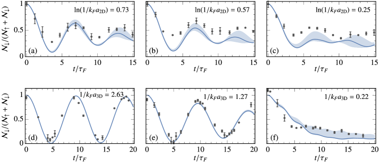
Figure 2: Rabi oscillations calculated using the TBM (solid lines) and compared with the data (black dots) from the 2D ¹⁷³Yb experiment Darkwah Oppong et al. (2019) (top row) and the 3D ⁶Li experiment Scazza et al. (2017) (bottom row). In the top row, $\Omega_{0}/E_{F}\simeq 0.95$ and $T/T_{F}\simeq 0.16$ while, from left to right, $\ln(1/k_{F}a_{\text{2D}})=$ $0.73,\,0.57,$ and $0.25$. In the bottom row, $\Omega_{0}/E_{F}\simeq 0.68$ and $T/T_{F}\simeq 0.13$ while, from left to right, $1/(k_{F}a)=$ $2.63,\,1.27,$ and $0.22$. The shaded regions correspond to the estimated uncertainty in the detuning around the repulsive polaron energy sup . In the top row, the data is calculated from the sole measurement of $\mathcal{N}_{\downarrow}(t)$, and the normalization of each data point to $\mathcal{N}_{\downarrow}(t=0)$ sup . We define the Fermi time $\tau_{F}\equiv 1/E_{F}$.

Model.—

To model the impurity dynamics in the 3D ⁶Li experiment of Ref. Scazza et al. (2017) and the 2D ¹⁷³Yb experiment of Ref. Darkwah Oppong et al. (2019), we use a unified notation where the dimensionality of momenta and sums are implicit. For clarity, even though we consider homonuclear systems, we introduce majority fermion creation operators $\hat{f}^{\dagger}_{\bf k}$ and impurity creation operators $\hat{c}^{\dagger}_{{\bf k},\sigma}$ with two different pseudo-spins $\sigma=\uparrow,\downarrow$ (Fig. 1). For a description of the precise relationship to atomic states in experiments, see the Supplemental Material sup .

The Hamiltonian we consider consists of four terms:

$$\hat{H}=\hat{H}_{0}+\hat{H}_{\uparrow}+\hat{H}_{\downarrow}+\hat{H}_{\Omega}.$$ (1)

The term $\hat{H}_{0}=\sum_{\bf k}(\epsilon_{{\bf k}}-\mu)\hat{f}_{\bf k}^{\dagger}\hat{f}_{\bf k}$ describes the medium in the absence of the impurity. Here, ${\bf k}$ is the particle momentum, $\epsilon_{{\bf k}}=|{\bf k}|^{2}/2m\equiv k^{2}/2m$ is the kinetic energy, and $m$ is the mass of both the fermions and the impurity (we work in units where $\hbar$ and the system volume or area are set to 1). We use a grand canonical formulation for the medium, with $\mu$ the corresponding chemical potential Liu et al. (2020a, b).

The impurity spin-$\sigma$ terms

$$\hat{H}_{\sigma}= \sum_{{\bf k}}\left[\epsilon_{{\bf k}}\hat{c}^{\dagger}_{{\bf k}\sigma}\hat{c}_{{\bf k}\sigma}+(\epsilon_{{\bf k}}/2+\nu_{\sigma})\hat{d}^{\dagger}_{{\bf k}\sigma}\hat{d}_{{\bf k}\sigma}\right]$$

$$+g_{\sigma}\sum_{{\bf k},{\bf q}}\left(\hat{d}^{\dagger}_{{\bf q}\sigma}\hat{c}_{{\bf q}-{\bf k}\sigma}\hat{f}_{{\bf k}}+\hat{f}^{\dagger}_{{\bf k}}\hat{c}^{\dagger}_{{\bf q}-{\bf k}\sigma}\hat{d}_{{\bf q}\sigma}\right),$$ (2)

describe the interaction of the impurity and majority fermions via the coupling into a closed channel with creation operator $\hat{d}^{\dagger}_{{\bf k}\sigma}$, where we have coupling constant $g_{\sigma}$ and closed-channel detuning $\nu_{\sigma}$. Renormalizing the model enables us to trade the bare parameters of the model — the detuning, the coupling constant, and an ultraviolet momentum cutoff — for the physical interaction parameters which parameterize the 2D and 3D impurity-majority fermion low-energy scattering amplitudes

$$f_{\text{2D}\sigma}(k) \simeq\frac{4\pi}{-\ln(k^{2}a^{2}_{\text{2D}\sigma})+R^{2}_{\text{2D}\sigma}k^{2}+i\pi},$$ (3a)

$$f_{\text{3D}\sigma}(k) \simeq\frac{1}{-a_{\text{3D}\sigma}^{-1}+ik},$$ (3b)

namely the 2D and 3D scattering lengths, $a_{\text{2D}\sigma}$ and $a_{\text{3D}\sigma}$, and a 2D range parameter $R_{\text{2D}\sigma}$ Levinsen and Parish (2013); sup . The presence of $R_{\text{2D}\sigma}$ in Eq. (3a) allows us to model the strongly energy-dependent scattering close to the ¹⁷³Yb orbital Feshbach resonance Zhang et al. (2015); Höfer et al. (2015); Pagano et al. (2015) in a 2D geometry. Conversely, we can safely neglect effective range corrections for the broad resonance, 3D case of ⁶Li. In what follows, we take the impurity spin-$\uparrow$ (spin-$\downarrow$) state to be strongly (weakly) interacting with the medium sup , as depicted in Fig. 1. To simplify notation, we therefore identify $a_{\rm 3D}\equiv a_{\rm 3D\uparrow}$, $a_{\rm 2D}\equiv a_{\rm 2D\uparrow}$, and $R_{\rm 2D}\equiv R_{\rm 2D\uparrow}$.

The radio-frequency Scazza et al. (2017) or optical Darkwah Oppong et al. (2019) fields that couple the impurities in states $\uparrow$ and $\downarrow$ are described within the rotating wave approximation:

$$\hat{H}_{\Omega}=\frac{\Omega_{0}}{2}\sum_{{\bf k}}\left(\hat{c}^{\dagger}_{{\bf k}\downarrow}\hat{c}_{{\bf k}\uparrow}+\hat{c}^{\dagger}_{{\bf k}\uparrow}\hat{c}_{{\bf k}\downarrow}\right)+\Delta\omega\,\hat{n}_{\downarrow}.$$ (4)

Here, $\hat{n}_{\sigma}=\sum_{\bf k}\left(\hat{c}^{\dagger}_{{\bf k}\sigma}\hat{c}_{{\bf k}\sigma}+\hat{d}^{\dagger}_{{\bf k}\sigma}\hat{d}_{{\bf k}\sigma}\right)$ is the spin-$\sigma$ impurity number operator, $\Omega_{0}$ is the (bare) Rabi coupling, and $\Delta\omega$ is the detuning from the bare $\downarrow$-$\uparrow$ transition.

Perturbative analysis.—

We can gain insight into the nature of the repulsive Fermi polaron by analyzing the quasiparticle peak in the spectrum at weak interactions and temperature $T=0$, such that the polaron is at rest. Focussing on the 3D case, in the limit $k_{F}a_{3D}\ll 1$ the polaron energy $E_{+}$ is given by the mean-field expression $E_{+}=\frac{4k_{F}a_{\rm 3D}}{3\pi}E_{F}+O(a_{\rm 3D}^{2})$ Bishop (1973), where $E_{F}=\frac{k_{F}^{2}}{2m}$ is the Fermi energy with $k_{F}$ the Fermi momentum. Thus, the quasiparticle state is pushed up into the continuum of scattering states that exists above zero energy in the case of attractive interactions. In particular, by performing a perturbative analysis sup , we find that the broadening of the quasiparticle peak [Fig. 1(b)] is dominated by the coupling to this continuum, such that the leading order behavior is

$$\Gamma\simeq\frac{8(k_{F}a_{\rm 3D})^{4}}{9\pi^{3}}E_{F}\simeq 0.029\,(k_{F}a_{\rm 3D})^{4}E_{F}.$$ (5)

This has two important consequences. First, at orders below $a_{\rm 3D}^{4}$, the quasiparticle behavior is indistinguishable from the case of truly repulsive interactions, where the lifetime would be infinite Bishop (1973); Pilati et al. (2010). In this regime, the repulsive polaron is adiabatically connected to the non-interacting impurity. Second, the contribution to the quasiparticle width from relaxation to the attractive branch is negligible in this limit, since it is dominated by three-body recombination Scazza et al. (2017) and takes the form $\Gamma_{3}\simeq 0.025(k_{F}a_{\rm 3D})^{6}E_{F}\,{\color[rgb]{0,0,0}\ll\Gamma}$ Petrov (2003). This illustrates that — within the perturbative regime — the finite quasiparticle lifetime arises from many-body dephasing processes that are manifestly distinct from relaxation to negative-energy states. Moreover, this cannot be viewed as momentum relaxation like in usual Fermi liquid theory Pines and Nozières (1966), since we are considering a zero-momentum quasiparticle.

Rabi oscillations as a probe of quasiparticles.—

We now argue that Rabi oscillations provide a sensitive probe of the repulsive polaron width (or quasiparticle lifetime). We focus on zero total momentum, since we are interested in decoherence effects beyond the standard momentum relaxation occurring in Fermi liquid theory Pines and Nozières (1966). At times $t\geq 0$, the impurity population in spin $\sigma$ is

$${\cal N}_{\sigma}(t)=\Tr[\hat{\rho}_{0}\hat{c}(t)\hat{n}_{\sigma}\hat{c}^{\dagger}(t)],$$ (6)

where $\hat{c}(t)$ is the impurity operator in the Heisenberg picture. Here, our initial state $\hat{c}(t=0)=\hat{c}_{{\bf 0}\downarrow}$ is chosen such that ${\cal N}_{\downarrow}(0)=1$ and ${\cal N}_{\uparrow}(0)=0$. The trace is over all states of the medium in the absence of the impurity, and we use the thermal density matrix $\hat{\rho}_{0}=\exp(-\beta\hat{H}_{0})/\Tr[\exp(-\beta\hat{H}_{0})]$ with $\beta\equiv 1/T$ (we set the Boltzmann constant to 1). Under the assumption that the initial zero-momentum component dominates such that $\hat{n}_{\downarrow}\simeq\hat{c}_{{\bf 0}\downarrow}^{\dagger}\hat{c}_{{\bf 0}\downarrow}$, we find sup

$${\cal N}_{\downarrow}(t)\simeq\int d\omega d\omega^{\prime}\,\tilde{A}_{\downarrow}(\omega)\tilde{A}_{\downarrow}(\omega^{\prime})e^{-i(\omega-\omega^{\prime})t},$$ (7)

where $\tilde{A}_{\downarrow}(\omega)$ is the spin-$\downarrow$ impurity spectral function in the presence of Rabi coupling. Taking the Rabi oscillations to be on resonance with the repulsive quasiparticle, i.e., $\Delta\omega=E_{+}$, we can furthermore approximate the spin-dependent impurity Green’s functions in the absence of Rabi coupling as $G_{\downarrow}(\omega)\simeq 1/(\omega-E_{+}+i\eta)$ and $G_{\uparrow}(\omega)\simeq Z/(\omega-E_{+}+i\Gamma)$, where $Z$ is the quasiparticle residue and $\eta$ is a convergence factor that implicitly carries the limit $\eta\to 0^{+}$. With these approximations and as long as $\Gamma\lesssim\sqrt{Z}\Omega_{0}$, we finally obtain sup

$${\cal N}_{\downarrow}(t) \simeq e^{-\Gamma t}\left[\frac{1}{2}+\frac{1}{2}\cos\left(t\sqrt{\Omega_{0}^{2}Z-\Gamma^{2}}\right)\right].$$ (8)

Equation (8) provides two valuable insights. First, the Rabi oscillation frequency $\Omega$ is related to the residue via $Z\simeq(\Omega^{2}+\Gamma^{2})/\Omega_{0}^{2}$, which provides a correction to the standard approximation of $Z\simeq(\Omega/\Omega_{0})^{2}$ Kohstall et al. (2012). Second, we see that the damping of Rabi oscillations is precisely the quasiparticle width $\Gamma$. This key result has been observed in experiment Scazza et al. (2017); Darkwah Oppong et al. (2019) but has previously lacked theoretical support.

Variational approach.—

We now turn to modelling the experimental Rabi oscillations. We apply the finite-temperature variational approach developed in Ref. Liu et al. (2019) in the context of Ramsey spectroscopy of impurities in a Fermi sea Cetina et al. (2016) (see also Ref. Parish and Levinsen (2016) for a related zero-temperature approach). The idea in this truncated basis method (TBM) is to introduce a time-dependent variational impurity operator $\hat{c}(t)=\hat{c}_{\uparrow}(t)+\hat{c}_{\downarrow}(t)$ that only approximately satisfies the Heisenberg equation of motion. This allows us to introduce an error operator $\hat{\epsilon}(t)\equiv i\partial_{t}\hat{{c}}(t)-\commutator*{\hat{{c}}(t)}{\hat{H}}$ and an associated error quantity $\Delta(t)\equiv\Tr[\hat{\rho}_{0}\hat{\epsilon}(t)\hat{\epsilon}^{\dagger}(t)]$. Our variational ansatz for the spin-$\sigma$ component of the impurity operator is inspired by the work of Chevy Chevy (2006) and corresponds to

$$\hat{{c}}_{\sigma}(t)\!=\!\alpha_{0}^{\sigma}(t)\hat{c}_{{\bf 0}\sigma}\!+\!\sum_{\bf k}\alpha_{{\bf k}}^{\sigma}(t)\hat{f}^{\dagger}_{\bf k}\hat{d}_{{\bf k}\sigma}\!+\!\sum_{{\bf k},{\bf q}}\alpha_{{\bf k}{\bf q}}^{\sigma}(t)\hat{f}^{\dagger}_{{\bf q}}\hat{f}_{{\bf k}}\hat{c}_{{\bf q}-{\bf k}\sigma}.$$ (9)

The variational operator consists of three terms: the bare impurity, the impurity bound to a fermion in a closed-channel dimer, and the impurity with a particle-hole excitation. The time dependence is entirely contained within the variational coefficients $\{\alpha\}$, allowing us to impose the minimization condition $\partialderivative*{\Delta(t)}{\dot{\alpha}^{\sigma*}_{j}(t)}=0$. Since the Rabi coupling is suddenly turned on at $t=0$, we can use the stationary solutions obtained from a set of linear equations for the expansion coefficients. This follows Ref. Liu et al. (2019) with straightforward modifications due to the two possible impurity spin states sup .

Following the application of an external driving field, we obtain the Rabi oscillations within our variational approach via Eq. (6). We show the resulting Rabi oscillations in Fig. 2 for a representative set of interaction strengths and temperatures $T/T_{F}$ in both two and three dimensions, where the Fermi temperature $T_{F}=E_{F}$. Here we set the detuning to match the theoretical repulsive polaron energy, with a small shift due to initial state interactions sup . The shaded regions illustrate the range of possible results that can be obtained by varying the detuning within the width of the repulsive polaron quasiparticle peak sup . This accounts for the Rabi oscillations being slightly off resonance in experiment due to the non-zero density of impurities, the density inhomogeneity within the trap, and other technical limitations.

Figure 2 demonstrates that our variational approach captures the Rabi oscillations between the bare impurity and the repulsive polaron in the 2D Darkwah Oppong et al. (2019) and 3D Scazza et al. (2017) experiments. We note that there is a small positive offset in the 2D data sup , which does not strongly affect the extracted Rabi parameters. Crucially, our variational ansatz does not incorporate any processes where the repulsive polaron decays into the attractive branch, because these involve additional particle-hole excitations Massignan and Bruun (2011) which are neglected in Eq. (9). Therefore, the consistency between our theoretical results and the experiments provides strong evidence that the decoherence in the Rabi oscillations — and hence the inverse quasiparticle lifetime $\Gamma$ — is physically dominated by the coupling to the continuum at positive energies, rather than by relaxation to the attractive branch. Given the fundamental differences between the two experiments Scazza et al. (2017); Darkwah Oppong et al. (2019), we expect this to be a generic feature of the mobile Fermi polaron with short-range attractive interactions.

Quasiparticle properties.—

We can further quantify the nature of the repulsive polaron by determining the frequency $\Omega$ and damping $\Gamma_{R}$ of the observed Rabi oscillations, which can be modelled approximately as Scazza et al. (2017):

$$\mathcal{N}_{\downarrow}(t)\simeq be^{-\Gamma_{\text{bg}}t}+(1-b)e^{-\Gamma_{R}t}\cos(\Omega t).$$ (10)

Here, $b$ is a dimensionless fitting parameter, while $\Gamma_{\text{bg}}$ can be regarded as a background decay rate of the spin-$\downarrow$ state. We see that Eq. (10) reduces to our theoretical expression in Eq. (8) if we set $b=1/2$ and $\Gamma_{\rm bg}=\Gamma_{R}$. In practice, we find that $\Gamma_{\rm bg}<\Gamma_{R}$ since there are scattering processes that can populate the spin-$\downarrow$ state without contributing to the damping of oscillations, and these are neglected in our approximation (7) .

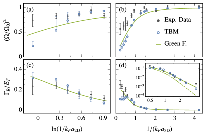
Figure 3: The extracted frequency $(\Omega/\Omega_{0})^{2}$ and damping $\Gamma_{R}$ of the Rabi oscillations as determined from the TBM (blue circles) and in the 2D (a,c) and 3D (b,d) experiments (black dots). The TBM error bars are derived from the uncertainty in detuning sup , which tends to increase the oscillation frequency. The extracted Rabi parameters are also compared with the quasiparticle residue $Z\simeq(\Omega/\Omega_{0})^{2}$ (top row) and quasiparticle inverse lifetime $\Gamma\simeq\Gamma_{R}$ (bottom row) obtained directly from the finite-temperature impurity Green’s function (green solid line). The TBM simulations are set to match the experimental parameters sup . Inset: Data in (d) plotted on a log-log scale, together with the result of a zero-temperature Green’s function calculation (green dashed line).

Using the fit provided in Eq. (10), we extract both $\Omega$ and $\Gamma_{R}$ from our simulated Rabi oscillations within the TBM and compare them with the experimental results, as depicted in Fig. 3. We also show the repulsive polaron residue $Z$ and inverse quasiparticle lifetime $\Gamma$ obtained directly from the impurity Green’s function $G_{\downarrow}(\omega)$, where the impurity self energy is calculated using ladder diagrams sup . Such an approach is equivalent to our spin-$\downarrow$ variational ansatz in Eq. (9) in the absence of Rabi coupling Liu et al. (2019), and similarly it does not include the contribution to the quasiparticle lifetime due to relaxation from the repulsive branch to lower lying states.

Referring to Fig. 3, we see that all three methods are in good agreement with each other for weak to intermediate interaction strengths. This is particularly evident for $\Gamma_{R}$ in Fig. 3(d), where the agreement spans two orders of magnitude. Here we find that the finite temperature of the Fermi gas leads to deviations from the perturbative result in Eq. (5), but the behavior is still markedly different from the momentum relaxation predicted by Fermi liquid theory Cetina et al. (2015). The observed agreement suggests that temperature predominantly affects the many-body dephasing via thermal fluctuations of the medium rather than through finite impurity momenta. In Fig. 3(a), the slightly elevated values of $(\Omega/\Omega_{0})^{2}$ compared to the expected residue $Z$ can be attributed to the strong Rabi driving ($\Omega_{0}/E_{F}\gtrsim 1$), such that the oscillation period approaches the formation time of the polaron.

At stronger repulsive interactions, there are more pronounced deviations as the repulsive polaron quasiparticle becomes less well defined and the effects of a finite impurity density in experiments are expected to be more important Scazza et al. (2017). In particular, it becomes increasingly difficult to extract quasiparticle properties from the Rabi oscillations once the quasiparticle width $\Gamma$ is comparable to $\Omega$, which is consistent with our theoretical analysis in Eq. (8). This accounts for the suppression of coherent oscillations in Fig. 2(f) as well as the anomalously low $\Gamma_{R}$ obtained from the TBM near unitarity in Fig. 3(d). Our results suggest that one could better probe the repulsive polaron quasiparticle lifetime at strong coupling by increasing the Rabi drive $\Omega_{0}$.

Conclusions.—

We have investigated the nature of the repulsive Fermi polaron in two and three dimensions. We have shown that both the quasiparticle lifetime and the residue can be probed by driving Rabi oscillations between weakly and strongly interacting impurity spin states. By simulating the Rabi oscillations in two fundamentally different experiments and by performing a perturbative analysis of the weak-coupling limit, we have demonstrated that the quasiparticle lifetime is determined by many-body dephasing within the upper repulsive branch and is thus typically much shorter than the lifetime of the repulsive branch itself. Our work provides an important benchmark for many-body numerical approaches Goulko et al. (2017) and it opens up the prospect of exploring a long-lived repulsive Fermi gas with novel excitations beyond the Fermi liquid paradigm.

SUPPLEMENTAL MATERIAL:
“Quasiparticle lifetime of the repulsive Fermi polaron”

Haydn S. Adlong,¹ Weizhe Edward Liu,^1,2 Francesco Scazza,³ Matteo Zaccanti,³ Nelson Darkwah Oppong,^4,5,6 Simon Fölling,^4,5,6 Meera M. Parish,^1,2 and Jesper Levinsen^1,2,

¹School of Physics and Astronomy, Monash University, Victoria 3800, Australia

²ARC Centre of Excellence in Future Low-Energy Electronics Technologies, Monash University, Victoria 3800, Australia

³Istituto Nazionale di Ottica del Consiglio Nazionale delle Ricerche (CNR-INO) and European Laboratory for Nonlinear Spectroscopy (LENS), 50019 Sesto Fiorentino, Italy

⁴Ludwig-Maximilians-Universität, Schellingstraße 4, 80799 München, Germany

⁵Max-Planck-Institut für Quantenoptik, Hans-Kopfermann-Straße 1, 85748 Garching, Germany

⁶Munich Center for Quantum Science and Technology (MCQST), Schellingstraße 4, 80799 München, Germany

I Model and scattering parameters

I.1 Model

In modelling the dynamics of impurities coupled to a Fermi sea, we use the following effective Hamiltonian

$$\hat{H}=\hat{H}_{0}+\hat{H}_{\Omega}+\hat{H}_{\uparrow}+\hat{H}_{\downarrow},$$ (S1)

where

$$\hat{H}_{0} =\sum_{\bf k}(\epsilon_{{\bf k}}-\mu)\hat{f}_{\bf k}^{\dagger}\hat{f}_{\bf k},$$ (S2a)

$$\hat{H}_{\Omega} =\frac{\Omega_{0}}{2}\sum_{{\bf k}}\left(\hat{c}^{\dagger}_{{\bf k}\downarrow}\hat{c}_{{\bf k}\uparrow}+\hat{c}^{\dagger}_{{\bf k}\uparrow}\hat{c}_{{\bf k}\downarrow}\right)+\Delta\omega\,\hat{n}_{\downarrow},$$ (S2b)

$$\hat{H}_{\sigma} =\sum_{{\bf k}}\left[\epsilon_{{\bf k}}\hat{c}^{\dagger}_{{\bf k}\sigma}\hat{c}_{{\bf k}\sigma}+(\epsilon_{{\bf k}}/2+\nu_{\sigma})\hat{d}^{\dagger}_{{\bf k}\sigma}\hat{d}_{{\bf k}\sigma}\right]+g_{\sigma}\sum_{{\bf k},{\bf q}}\left(\hat{d}^{\dagger}_{{\bf q}\sigma}\hat{c}_{{\bf q}/2-{\bf k},\sigma}\hat{f}_{{\bf q}/2+{\bf k}}+\hat{f}^{\dagger}_{{\bf q}/2+{\bf k}}\hat{c}^{\dagger}_{{\bf q}/2-{\bf k},\sigma}\hat{d}_{{\bf q}\sigma}\right).$$ (S2c)

The meaning of the various symbols is discussed in the main text.

I.2 Relation between Hamiltonian operators and experimental atomic states

In the 2D ¹⁷³Yb experiment of Ref. Darkwah Oppong et al. (2019), the states of the atoms are defined by the electronic state, with ground state ${}^{1}S_{0}$ and long-lived excited state ${}^{3}P_{0}$ (i.e., the “clock” state), as well as the nuclear-spin state with $m_{F}\in\{-5/2,-3/2,\ldots,+5/2\}$. The majority $\hat{f}_{\bf k}^{\dagger}$ atoms exist in the $m_{F}=+5/2$ ground state, which acts as a bath for the weakly interacting $\hat{c}^{\dagger}_{{\bf k}\downarrow}$ and resonantly interacting $\hat{c}^{\dagger}_{{\bf k}\uparrow}$ impurities in the $m_{F}=-3/2$ ground state and $m_{F}=-5/2$ ‘clock’ state, respectively. Interactions between the $\hat{c}^{\dagger}_{{\bf k}\uparrow}$ and $\hat{f}_{\bf k}^{\dagger}$ atoms are tunable through an orbital Feshbach resonance Zhang et al. (2015) as has been demonstrated experimentally Höfer et al. (2015); Pagano et al. (2015).

On the other hand, the 3D experiment of Ref. Scazza et al. (2017) involves ⁶Li atoms in the three lowest Zeeman levels. The majority $\hat{f}_{\bf k}^{\dagger}$ atoms exist in the lowest Zeeman level, while the weakly interacting $\hat{c}^{\dagger}_{{\bf k}\downarrow}$ and resonantly interacting $\hat{c}^{\dagger}_{{\bf k}\uparrow}$ impurities occupy the second-lowest and third-lowest Zeeman levels respectively. Owing to two off-centered broad Feshbach resonances, the scattering between the $\hat{c}^{\dagger}_{{\bf k}\uparrow}$ and $\hat{f}_{\bf k}^{\dagger}$ atoms can be resonantly enhanced while only moderately increasing the comparatively weak interactions between the $\hat{c}^{\dagger}_{{\bf k}\downarrow}$ and $\hat{f}_{\bf k}^{\dagger}$ atoms Scazza et al. (2017).

I.3 Scattering parameters

Within the model in Eq. (S1), fermions of the same spin do not interact and the two spin states of the impurity are only coupled through the light-field. Ignoring for the moment the light-field (i.e., setting $\Omega_{0}=0$), we calculate the vacuum spin-dependent impurity-fermion $T$ matrix, which characterizes the interactions between the majority fermions and a particular spin state of the impurity. This yields

$$T_{\sigma}(E)=\left[\frac{E-\nu_{\sigma}}{g^{2}_{\sigma}}-\sum_{{\bf k}}^{\Lambda}\frac{1}{E-2\epsilon_{{\bf k}}}\right]^{-1},$$ (S3)

where $E$ is the collision energy and $\Lambda$ is the ultraviolet cutoff.

To proceed, we compare the scattering $T$ matrix with the 2D and 3D scattering amplitudes using $f_{2{\rm D}\sigma}(k)=mT_{\sigma}(E)$ and $f_{3{\rm D}\sigma}(k)=-\frac{m}{4\pi}T_{\sigma}(E)$, with $E=k^{2}/m$. The scattering amplitudes at low energy are known to take the forms

$$f_{\text{2D}\sigma}(k) \simeq\frac{4\pi}{-\ln(k^{2}a^{2}_{\text{2D}\sigma})+R^{2}_{\text{2D}\sigma}k^{2}+i\pi},$$ (S4a)

$$f_{\text{3D}\sigma}(k) \simeq-\frac{1}{a_{\text{3D}\sigma}^{-1}+R_{\text{3D}\sigma}k^{2}+ik}.$$ (S4b)

By comparing Eq. (S3) with the low-energy scattering amplitudes, we obtain the renormalized scattering parameters. In 2D, this results in

$$\frac{\nu_{\sigma}+E_{2\sigma}}{g^{2}_{\sigma}}=\sum_{{\bf k}}^{\Lambda}\frac{1}{E_{2\sigma}+2\epsilon_{{\bf k}}},\qquad R_{\text{2D}\sigma}^{2}=\frac{4\pi}{m^{2}g^{2}_{\sigma}},$$ (S5)

where $a_{{\rm 2D}\sigma}$ is the scattering length, $R_{2{\rm D}\sigma}$ is the effective range Kirk and Parish (2017), and $E_{2\sigma}$ is the binding energy of the two-body bound state that exists for all interactions in 2D:

$$E_{2\sigma}=\frac{1}{mR^{2}_{\text{2D}\sigma}}W\left(\frac{R^{2}_{\text{2D}\sigma}}{a^{2}_{\text{2D}\sigma}}\right),$$ (S6)

with $W$ the Lambert $W$ function. In 3D, we have

$$\frac{m}{4\pi a_{\text{3D}\sigma}}=-\frac{\nu_{\sigma}}{g^{2}_{\sigma}}+\sum_{{\bf k}}^{\Lambda}\frac{1}{2\epsilon_{{\bf k}}},\qquad R_{\text{3D}\sigma}=\frac{4\pi}{m^{2}g_{\sigma}^{2}},$$ (S7)

where $a_{{\rm 3D}\sigma}$ is the scattering length and $R_{3{\rm D}\sigma}$ is a range parameter Gurarie and Radzihovsky (2007). In this case, we only have a bound state when $a_{{\rm 3D}\sigma}>0$, with corresponding binding energy

$$E_{3\sigma}=\frac{\left[\sqrt{1+4R_{3{\rm D}\sigma}/a_{3{\rm D}\sigma}}-1\right]^{2}}{4m{R_{3{\rm D}\sigma}^{2}}}.$$ (S8)

Through this procedure, we have related the bare interaction parameters $g$, $\Lambda$, and $\nu$ to the physical parameters, the scattering length $a$ and effective range $R$, which characterises the relevant Feshbach resonance. For the broad Feshbach resonances in ⁶Li we use $R_{\text{3D}\sigma}=0$ for both spin states. For the orbital Feshbach resonance in quasi-2D, the description of the effective range is somewhat more complicated, as discussed in the following.

I.4 Effective model for scattering at an orbital Feshbach resonance in the presence of confinement

We now discuss how the scattering parameters, $a_{\text{2D}\sigma}$ and $R_{\text{2D}\sigma}$, of the ¹⁷³Yb experiment are determined. The orbital Feshbach resonance is known to lead to a strongly energy dependent scattering Zhang et al. (2015), which is well approximated by the introduction of a 3D effective range Xu et al. (2016). Furthermore, quasi-2D confinement generally leads to a non-trivial energy dependence of the effective 2D scattering amplitude even for a broad Feshbach resonance Petrov and Shlyapnikov (2001); for strong confinement, this energy dependence can be modelled by the introduction of a 2D effective range Levinsen and Parish (2013). Thus, we use the effective range in our model to provide the simplest possible description of both the orbital Feshbach resonance and the confinement. This greatly simplifies the numerical simulations of Rabi oscillations, since it drastically reduces the possible degrees of freedom in the problem.

We now describe the possible scattering channels in ¹⁷³Yb atoms close to an orbital Feshbach resonance, following the analysis in Ref. Zhang et al. (2015). We focus on the two electronic orbitals described above (denoted here by $\ket{g}$ and $\ket{e}$) as well as two particular nuclear spin states (denoted here by $\ket{\Downarrow}$ and $\ket{\Uparrow}$). These states form the open channel $\ket{o}\equiv\ket{g\Uparrow,e\Downarrow}$ and the closed channel $\ket{c}\equiv\ket{e\Uparrow,g\Downarrow}$, which are detuned by $\delta=\Delta\mu B$, where $\Delta\mu=h\times 554\,\mathrm{Hz}/\mathrm{G}$ Darkwah Oppong et al. (2019) is the differential Zeeman shift and $B$ is the magnetic field strength in Gauss. The interactions in this system are not diagonal in the open- and closed-channel basis, but instead proceed via the triplet $(+)$ and singlet $(-)$ channels, with $\ket{\pm}\equiv\frac{1}{\sqrt{2}}(\ket{o}\pm\ket{c})$. Associated with the singlet and triplet interactions are the singlet and triplet scattering lengths $a_{\pm}$ Zhang et al. (2015) and effective ranges $r_{\pm}$ Höfer et al. (2015).

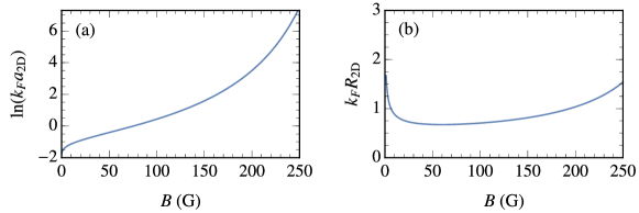
Figure S1: The open channel 2D scattering length (a) and 2D effective range (b) as a function of magnetic field strength (in Gauss). These parameters are used to create an effective 2D two-channel model description of scattering at an orbital Feshbach resonance in the presence of confinement. To match Ref. Darkwah Oppong et al. (2019) we use $\omega_{z}=2\pi\times 37.1\,\mathrm{kHz}$.

In the experiment Darkwah Oppong et al. (2019), the ¹⁷³Yb atoms were confined to move in a 2D plane with a harmonic potential $V(z)=\frac{1}{2}m\omega_{z}^{2}z^{2}$ acting in the transverse direction. Reference Darkwah Oppong et al. (2019) used this to extend the theoretical analysis of quasi-2D scattering in Refs. Petrov and Shlyapnikov (2001); Bloch et al. (2008) to derive an effective scattering amplitude of the form in Eq. (S4a). For the weakly interacting $\downarrow$ state, it was found that $\ln(k_{F}a_{\text{2D}\downarrow})\simeq-4.9(1)$ Darkwah Oppong et al. (2019). In this case, the dependence on $R_{\text{2D}\downarrow}$ is strongly suppressed, and we simply take $R_{\text{2D}\downarrow}=0$. For the case of strong interactions, the open channel scattering amplitude was found to be given by Darkwah Oppong et al. (2019)

$$f_{\text{q2D}}(E) =2\sqrt{2\pi}\frac{l_{z}\left(\tilde{a}^{-1}_{-}-\frac{mr_{-}E}{2}\right)+l_{z}\left(\tilde{a}^{-1}_{+}-\frac{mr_{+}E}{2}\right)-2\mathcal{F}\left(\frac{-E+\delta}{\omega_{z}}\right)}{\left\{\begin{multlined}-\mathcal{F}\left(\frac{-E+\delta}{\omega_{z}}\right)\left[l_{z}(\tilde{a}^{-1}_{-}-\frac{mr_{-}E}{2})+l_{z}(\tilde{a}^{-1}_{+}-\frac{mr_{+}E}{2})-2\mathcal{F}\left(-\frac{E}{\omega_{z}}\right)\right]\\ -\mathcal{F}\left(-\frac{E}{\omega_{z}}\right)\left[l_{z}(\tilde{a}^{-1}_{-}-\frac{mr_{-}E}{2})+l_{z}(\tilde{a}^{-1}_{+}-\frac{mr_{+}E}{2})\right]+2l_{z}^{2}(\tilde{a}^{-1}_{-}-\frac{mr_{-}E}{2})(\tilde{a}^{-1}_{+}-\frac{mr_{+}E}{2})\end{multlined}-\mathcal{F}\left(\frac{-E+\delta}{\omega_{z}}\right)\left[l_{z}(\tilde{a}^{-1}_{-}-\frac{mr_{-}E}{2})+l_{z}(\tilde{a}^{-1}_{+}-\frac{mr_{+}E}{2})-2\mathcal{F}\left(-\frac{E}{\omega_{z}}\right)\right]\\ -\mathcal{F}\left(-\frac{E}{\omega_{z}}\right)\left[l_{z}(\tilde{a}^{-1}_{-}-\frac{mr_{-}E}{2})+l_{z}(\tilde{a}^{-1}_{+}-\frac{mr_{+}E}{2})\right]+2l_{z}^{2}(\tilde{a}^{-1}_{-}-\frac{mr_{-}E}{2})(\tilde{a}^{-1}_{+}-\frac{mr_{+}E}{2})\right\}},$$ (S11)

where $l_{z}=1/\sqrt{m\omega_{z}}$ and $\tilde{a}_{\pm}^{-1}=a^{-1}_{\pm}-\frac{r_{\pm}}{4l_{z}^{2}}\left(1-\delta/\omega_{z}\right)$. Here, $\mathcal{F}$ is a transcendental function defined by Bloch et al. (2008)

$$\mathcal{F}(x)=\int_{0}^{\infty}\frac{du}{\sqrt{4\pi u^{3}}}\left[1-\frac{e^{-xu}}{\sqrt{(1-e^{-2u})/2u}}\right],$$ (S12)

and the energy is measured with respect to the quasi-2D zero point energy.

To extract an effective low-energy open-channel 2D scattering length and effective range for the strongly interacting spin-$\uparrow$ impurity case, we perform a low energy expansion of Eq. (S11) and compare it with the standard form of the low-energy scattering amplitude, Eq. (S4a). In the following, we use the notation $a_{\text{2D}}\equiv a_{\text{2D}\uparrow}$ and $R_{\text{2D}}\equiv R_{\text{2D}\uparrow}$, as in the main text. Assuming that $\delta\gg|E|$ (i.e., that we are not close to $B=0$) we find the 2D scattering length Darkwah Oppong et al. (2019)

$$a_{\text{2D}}=l_{z}\sqrt{\frac{\pi}{D}}\exp[-\sqrt{2\pi}\frac{l_{z}^{2}(\tilde{a}_{-}\tilde{a}_{+})^{-1}-\frac{1}{2}(l_{z}\tilde{a}_{-}^{-1}+l_{z}\tilde{a}_{+}^{-1})\mathcal{F}\left(\frac{\delta}{\omega_{z}}\right)}{l_{z}\tilde{a}_{-}^{-1}+l_{z}\tilde{a}_{+}^{-1}-2\mathcal{F}\left(\frac{\delta}{\omega_{z}}\right)}],$$ (S13)

where $D\simeq 0.905$ Petrov and Shlyapnikov (2001). The 2D effective range takes the form

$$\left(\frac{R_{\text{2D}}}{l_{z}}\right)^{2} =\ln 2-\frac{\sqrt{2\pi}\left\{l_{z}^{-1}r_{+}\left[l_{z}\tilde{a}_{-}^{-1}-\mathcal{F}\left(\frac{\delta}{\omega_{z}}\right)\right]^{2}+l_{z}^{-1}r_{-}\left[l_{z}\tilde{a}_{+}^{-1}-\mathcal{F}\left(\frac{\delta}{\omega_{z}}\right)\right]^{2}+\left[l_{z}\tilde{a}_{-}^{-1}-l_{z}\tilde{a}_{+}^{-1}\right]^{2}\mathcal{F}^{\prime}\left(\frac{\delta}{\omega_{z}}\right)\right\}}{\left(l_{z}\tilde{a}_{-}^{-1}+l_{z}\tilde{a}_{+}^{-1}-2\mathcal{F}\left(\frac{\delta}{\omega_{z}}\right)\right)^{2}},$$ (S14)

where $\mathcal{F}^{\prime}$ is the first derivative of $\mathcal{F}$.

Figure S1 shows the extracted scattering parameters using the experimentally determined values for all parameters Darkwah Oppong et al. (2019) (see also Ref. Höfer et al. (2015)). We see that indeed the change of the magnetic field provides a means to tune the interactions via $a_{{\rm 2D}}$. On the other hand, the effective range is not strongly dependent on magnetic field — indeed, the effective range is approximately constant ($k_{F}R_{\text{2D}}\sim 1$) within the magnetic field strengths of interest to the present work.

In general, we find that the 2D effective range is able to highly accurately capture the physics of the orbital Feshbach resonance and the confinement in the domain of interaction strengths used in Ref. Darkwah Oppong et al. (2019). This is shown in Fig. S2, where we show the near perfect agreement between the full theory model Darkwah Oppong et al. (2019) and our effective model in calculating the energy of the Fermi polaron.

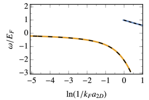
Figure S2: The attractive (orange) and repulsive (blue) Fermi polaron energy as calculated through our effective two-channel model description of an orbital Feshbach resonance in the presence of confinement. The energies are highly consistent with the full theory calculation of the polaron energies (black) from Ref. Darkwah Oppong et al. (2019). The curves are calculated at temperature $T/T_{F}=0.16$.

II Finite temperature variational approach for impurity dynamics

In order to model the dynamics of the Rabi oscillations and the impurity spectral response, we use the finite-temperature Truncated Basis Method (TBM) developed in Refs. Parish and Levinsen (2016); Liu et al. (2019). The basic details of this method are discussed in the main text. Our ansatz for the impurity operator is

$$\hat{c}(t)= \sum_{\sigma}\Bigg{[}\alpha_{0}^{\sigma}(t)\hat{c}_{{\bf 0}\sigma}+\sum_{\bf k}\alpha_{{\bf k}}^{\sigma}(t)\hat{f}^{\dagger}_{\bf k}\hat{d}_{{\bf k}\sigma}+\sum_{{\bf k},{\bf q}}\alpha_{{\bf k}{\bf q}}^{\sigma}(t)\hat{f}^{\dagger}_{{\bf q}}\hat{f}_{{\bf k}}\hat{c}_{{\bf q}-{\bf k}\sigma}\Bigg{]},$$ (S15)

where, for simplicity, we consider a vanishing total momentum. As discussed in the main text, we may quantify the error incurred in the Heisenberg equation of motion by introducing the error operator $\hat{\epsilon}(t)\equiv i\partial_{t}\hat{c}(t)-\commutator*{\hat{c}(t)}{\hat{H}}$ and the associated error quantity $\Delta(t)\equiv\Tr[\hat{\rho}_{0}\hat{\epsilon}(t)\hat{\epsilon}^{\dagger}(t)]$. Using the minimization condition $\partialderivative*{\Delta(t)}{\dot{\alpha}^{\sigma*}_{j}(t)}=0$ with respect to the variational coefficients $\{\alpha_{j}\}$, we arrive at

$$E\alpha^{\uparrow}_{0} =g_{\uparrow}\sum_{{\bf q}}\alpha^{\uparrow}_{{\bf q}}\Tr[\hat{\rho}_{0}\hat{f}^{\dagger}_{{\bf q}}\hat{f}_{{\bf q}}]+\frac{\Omega_{0}}{2}\alpha^{\downarrow}_{0}$$ (S16a)

$$(E-\varepsilon_{{\bf q}\uparrow})\alpha^{\uparrow}_{{\bf q}} =g_{\uparrow}\alpha^{\uparrow}_{0}+g_{\uparrow}\sum_{{\bf k}}\alpha^{\uparrow}_{{\bf k}{\bf q}}\Tr[\hat{\rho}_{0}\hat{f}_{{\bf k}}\hat{f}^{\dagger}_{{\bf k}}]$$ (S16b)

$$(E-\varepsilon_{{\bf k}{\bf q}})\alpha^{\uparrow}_{{\bf k}{\bf q}} =g_{\uparrow}\alpha^{\uparrow}_{{\bf q}}+\frac{\Omega_{0}}{2}\alpha^{\downarrow}_{{\bf k}{\bf q}}$$ (S16c)

$$(E-\Delta\omega)\alpha^{\downarrow}_{0} =g_{\downarrow}\sum_{{\bf q}}\alpha^{\downarrow}_{{\bf q}}\Tr[\hat{\rho}_{0}\hat{f}^{\dagger}_{{\bf q}}\hat{f}_{{\bf q}}]+\frac{\Omega_{0}}{2}\alpha^{\uparrow}_{0}$$ (S16d)

$$(E-\varepsilon_{{\bf q}\downarrow}-\Delta\omega)\alpha^{\downarrow}_{{\bf q}} =g_{\downarrow}\alpha^{\downarrow}_{0}+g_{\downarrow}\sum_{{\bf k}}\alpha^{\downarrow}_{{\bf k}{\bf q}}\Tr[\hat{\rho}_{0}\hat{f}_{{\bf k}}\hat{f}^{\dagger}_{{\bf k}}]$$ (S16e)

$$(E-\varepsilon_{{\bf k}{\bf q}}-\Delta\omega)\alpha^{\downarrow}_{{\bf k}{\bf q}} =g_{\downarrow}\alpha^{\downarrow}_{{\bf q}}+\frac{\Omega_{0}}{2}\alpha^{\uparrow}_{{\bf k}{\bf q}}.$$ (S16f)

Here we have taken the stationary condition since our Hamiltonian is time-independent,

$$\alpha^{\sigma}_{j}(t)=\alpha^{\sigma}_{j}(0)e^{-iEt}\equiv\alpha^{\sigma}_{j}e^{-iEt},$$ (S17)

and defined $\varepsilon_{{\bf q}\sigma}\equiv\nu_{\sigma}-\epsilon_{{\bf q}}/2$ and $\varepsilon_{{\bf k}{\bf q}}\equiv\epsilon_{{\bf q}-{\bf k}}+\epsilon_{{\bf k}}-\epsilon_{{\bf q}}$.

Equation (S16) represents a set of linear integral equations that define the time dependence of the variational coefficients $\{\alpha_{j}\}$. It is quite similar to the corresponding set of equations derived in Refs. Parish and Levinsen (2016); Liu et al. (2019). However, here we account for temperature, initial-state interactions, and the Rabi coupling between the two impurity spin states. Diagonalizing Eq. (S16) yields eigenvectors $\{\alpha_{j}^{(l)}\}$ and corresponding eigenvalues $E_{l}$. In what follows it is useful to write the eigenvectors as the union of the spin-$\uparrow$ and spin-$\downarrow$ components, i.e., $\{\alpha_{j}^{(l)}\}=\{\alpha^{\uparrow(l)}_{j}\}\cup\{\alpha^{\downarrow(l)}_{j}\}.$

The solutions of Eq. (S16) allow us to obtain stationary impurity operators

$$\hat{\phi}^{(l)}\equiv\sum_{j}\alpha_{j}^{(l)}\hat{O}_{j},$$ (S18)

where the impurity basis operators $\{\hat{O}_{j}\}=\{\hat{c}_{{\bf 0}\uparrow},\hat{f}^{\dagger}_{\bf k}\hat{d}_{{\bf k}\uparrow},\hat{f}^{\dagger}_{{\bf q}}\hat{f}_{{\bf k}}\hat{c}_{{\bf q}-{\bf k}\uparrow},\hat{c}_{{\bf 0}\downarrow},\hat{f}^{\dagger}_{\bf k}\hat{d}_{{\bf k}\downarrow},\hat{f}^{\dagger}_{{\bf q}}\hat{f}_{{\bf k}}\hat{c}_{{\bf q}-{\bf k}\downarrow}\}$ are those introduced in Eq. (S15). These all satisfy $\Tr[\hat{\rho}_{0}\hat{O}_{j}\hat{O}^{\color[rgb]{0,0,0}{\dagger}}_{k}]=0$ when $j\neq k$, since the trace is over medium-only states. This in turn allows us to normalize the stationary solutions according to

$$\Tr[\hat{\rho}_{0}\hat{\phi}^{(l)}\hat{\phi}^{(m){\dagger}}]=\delta_{lm}.$$ (S19)

Using this, the impurity annihilation operator in Eq. (S15) can be expressed as

$$\hat{c}(t)=\sum_{l}\Tr[\hat{\rho}_{0}\hat{c}(0)\hat{\phi}^{(l)\dagger}]\hat{\phi}^{(l)}e^{-iE_{l}t}=\sum_{l}\alpha_{0}^{{\color[rgb]{0,0,0}\downarrow}(l)*}\hat{\phi}^{(l)}e^{-iE_{l}t},$$ (S20)

where the initial impurity operator $\hat{c}(0)=\hat{c}_{{\bf 0}\downarrow}$. We take a bare impurity as the initial state even though there are initial-state interactions, since the simulations yield essentially the same result as when we use a weakly interacting polaron. We presume this is because the weakly interacting polaron forms quickly (on a time scale set by $a_{\mathrm{3D}\downarrow}^{2}$ in 3D) once we start the dynamics.

Finally, we discuss the character of the medium-only states appearing in Eq. (S16). Assuming that the interactions between the initial $\downarrow$ impurity and the medium particles are negligible (as is the case in the experiments Scazza et al. (2017); Darkwah Oppong et al. (2019)), we may take the medium states to be thermal eigenstates at temperature $T$. Therefore, we have

$$\Tr[\hat{\rho}_{0}\hat{f}^{\dagger}_{{\bf q}}\hat{f}_{{\bf q}}]\equiv\expectationvalue{\hat{f}^{\dagger}_{{\bf q}}\hat{f}_{{\bf q}}}_{\beta}=n_{F}(\epsilon_{{\bf q}})$$ (S21)

where $\beta$ is the inverse temperature and $n_{F}$ is the Fermi-Dirac distribution function:

$$n_{F}(\epsilon_{{\bf q}})\equiv\Tr[\hat{\rho}_{0}\hat{f}^{\dagger}_{\bf q}\hat{f}_{\bf q}]=\frac{1}{e^{\beta(\epsilon_{{\bf q}}-\mu)}+1}.$$ (S22)

The chemical potential $\mu$ is related to the medium density $n$ via

$$n=\sum_{\bf q}n_{F}(\epsilon_{{\bf q}})=\begin{cases}-\left(\frac{m}{2\pi\beta}\right)^{3/2}{\rm Li}_{3/2}(-e^{\beta\mu})&\rm(3D)\\[5.0pt] \frac{m}{2\pi\beta}\ln(1+e^{\beta\mu})&\mbox{(2D)}\end{cases}$$ (S23)

where ${\rm Li}$ is the polylogarithm. The density is related to the Fermi energy via

$$E_{F}=\frac{k_{F}^{2}}{2m}=\begin{cases}\frac{(6\pi^{2}n)^{2/3}}{2m}&\rm(3D)\\ \frac{4\pi n}{2m}&\rm{(2D)}\end{cases}$$ (S24)

II.1 Impurity spectral function

In the limit of a weak Rabi coupling, we can obtain the spin-$\uparrow$ impurity spectral function within linear response:

$$A_{\uparrow}(\omega)\simeq\sum_{l}|\alpha^{\uparrow(l)}_{0}|^{2}\delta(\omega-E_{l}),$$ (S25)

where the variational equations in Eq. (S16) are solved at $\Omega_{0}=0$. In practice, the spin-$\downarrow$ impurity interacts weakly with the medium, and thus the spectral function can be measured by driving transitions from the initial (nearly) non-interacting spin-$\downarrow$ impurity state into the spin-$\uparrow$ state. Indeed, this has been done in both experiments Scazza et al. (2017); Darkwah Oppong et al. (2019).

Since the solution of Eq. (S16) are discrete, we convolve the resulting spectrum with a Gaussian to yield

$$I(\omega) =\sum_{l}|\alpha^{\uparrow(l)}_{0}|^{2}g(\omega-E_{l}).$$ (S26)

Convolution of the spectrum in this case has the added benefit of enabling one to approximately model the finite duration of the pulses used in experiment.

II.2 Simulating Rabi oscillations

The Rabi oscillations are defined by

$${\cal N}_{\downarrow}(t)=\expectationvalue{\hat{c}(t)\hat{n}_{\downarrow}\hat{c}^{\dagger}(t)}_{\beta}.$$ (S27)

We will take as our initial condition that $\hat{c}({\color[rgb]{0,0,0}t=0})=\hat{c}_{{\bf 0}\downarrow}$, i.e., the impurity is initially in a bare spin-$\downarrow$ state, which means that the impurity number is ${\cal N}_{\downarrow}+{\cal N}_{\uparrow}=1$ at all times. The Rabi oscillations are then given by

$${\cal N}_{\downarrow}(t) \simeq\Tr[\hat{\rho}_{0}\hat{c}_{\downarrow}(t)\hat{n}_{\downarrow}\hat{c}^{\dagger}_{\downarrow}(t)]=\sum_{j}{\color[rgb]{0,0,0}\expectationvalue*{\hat{O}_{j}\hat{n}_{\downarrow}\hat{O}^{\dagger}_{j}}_{\beta}}\bigg{|}\sum_{l}\alpha_{0}^{\downarrow(l)^{*}}e^{-iE_{l}t}\alpha_{j}^{\downarrow(l)}\bigg{|}^{2}.$$ (S28)

With the exception of detuning, all of the parameters used to define the Rabi oscillations are provided from the relevant experiment. The detuning in experiment is set to address the repulsive polaron peak, and to match this procedure, we use a calculated detuning such that the Rabi oscillations address the theoretically obtained spin-$\uparrow$ repulsive polaron. Due to small but finite initial state interactions, this detuning must take into account the energy of the spin-$\downarrow$ impurities. This is achieved by assuming the spin-$\downarrow$ impurities exist as zero-momentum repulsive polarons with a narrow spectral width. Owing to this assumption, combined with thermal fluctuations, a finite density of impurities and experimental limitations, we place an uncertainty on the detuning (see Fig. S3). This requires that we simulate Rabi oscillations over the range of possible detunings. The parameters used in the simulations of the Rabi oscillations in Figs. 2 and 3 can be found in Table S1.

We find that the inclusion of initial state interactions leads to a small reduction in the damping of the Rabi oscillations. This can be understood from the fact that in the limit in which the spin states have equal interactions, spin-symmetry implies that the Rabi oscillations would be undamped and oscillate at the bare Rabi frequency.

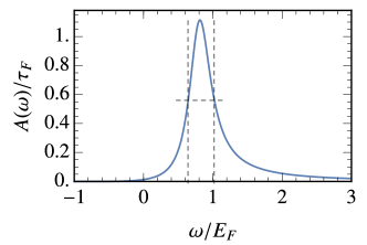
Figure S3: Example of the calculation of the uncertainty in the detuning of Rabi oscillations onto the repulsive polaron. We show the spectral function of the repulsive polaron in the 2D ¹⁷³Yb experiment of Ref. Darkwah Oppong et al. (2019) (solid line), with the dashed lines indicating the full-width half-maxima. The detuning is set between these half-maxima, leading to the uncertainty shown in Fig. 2 in the main text. The shown spectral function is for $\ln(1/k_{F}a_{\text{2D}})=0.41$, $k_{F}R_{\text{2D}}=0.69$ and $T/T_{F}=0.16$.

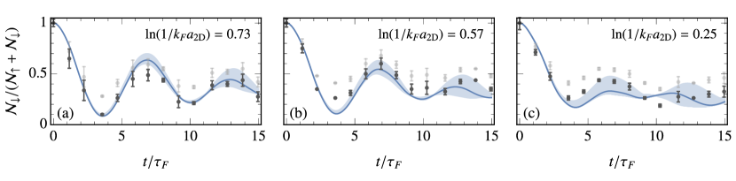
Figure S4: Comparison of theory (blue solid lines) of Fig. 2(a)-(c) in the manuscript and the experimental data (black circles) with a constant offset of $0.2$ removed and normalized to the value at time $t=0$. The light-gray circles correspond to the unmodified data in the main text.

II.3 Finite offset in the Rabi oscillation measurement of the 2D experiment

As noted in the main text, there is a slight disagreement in the amplitude of the Rabi oscillations in the 2D experiment Darkwah Oppong et al. (2019) and our variational approach. This disagreement can be explained with a constant offset $\epsilon>0$ of the $\mathcal{N}_{\downarrow}$ measurement in the experiment. In our work, the relative population $\mathcal{N}_{\downarrow}/(\mathcal{N}_{\downarrow}+\mathcal{N}_{\uparrow})$ of the 2D experiment is inferred from the sole measurement of $\mathcal{N}_{\downarrow}(t)$ and

$$\mathcal{N}_{\downarrow}\left/(\mathcal{N}_{\downarrow}+\mathcal{N}_{\uparrow})\right.\approx\mathcal{N}_{\downarrow}\left/[\mathcal{N}_{\downarrow}(t=0)+\mathcal{N}_{\uparrow}(t=0)]\right.\approx\mathcal{N}_{\downarrow}/[\mathcal{N}_{\downarrow}(t=0)+0]=\mathcal{N}_{\downarrow}\left/\mathcal{N}_{\downarrow}(t=0)\right..$$ (S29)

Thus, a constant offset in the measurement of $\mathcal{N}_{\downarrow}$ changes the relative population as

$$\mathcal{N}_{\downarrow}\left/\mathcal{N}_{\downarrow}(t=0)\right.\rightarrow(\mathcal{N}_{\downarrow}+\epsilon)\left/[\mathcal{N}_{\downarrow}(t=0)+\epsilon]\right.=\mathcal{N}_{\downarrow}\left/[\mathcal{N}_{\downarrow}(t=0)+\epsilon]\right.+\epsilon\left/[\mathcal{N}_{\downarrow}(t=0)+\epsilon]\right.,$$ (S30)

which directly shows how the mean of the relative population is artificially increased by $\epsilon/[\mathcal{N}_{\downarrow}(t=0)+\epsilon]$ and the amplitude is artificially reduced by the additional term $\epsilon$ in the denominator.

The offset $\epsilon$ in the experimental data originates from the detection method, for which the majority Fermi sea is removed, but a finite number of remaining majority atoms contributes a positive spurious signal to the measurement of $\mathcal{N}_{\downarrow}$. This contribution is independent of $t$ and we estimate $\epsilon\lesssim 0.2\,\mathcal{N}_{\downarrow}$ from a reevaluation of the existing data of Ref. Darkwah Oppong et al. (2019). In Fig. S4, we illustrate how the removal of such an offset considerably improves the agreement between experiment and the variational approach. However, we have chosen not to subtract $\epsilon$ from the data in Fig. 2 of the main text as we lack a precise number for each data set.

Table S1: Parameters used for obtaining the theoretical curves and simulations shown in Figs. 2 and 3, matching the experimental ones from Refs. Darkwah Oppong et al. (2019) and Scazza et al. (2017). Experimental uncertainties are given in parenthesis were applicable. Note that the 3D effective range is always zero.

		Fig. 2								Fig. 3
		(a)	(b)	(c)		(d)	(e)	(f)		(a), (c)		(b), (d)
Interaction parameter	$\ln(1/k_{F}a_{\mathrm{2D}\uparrow})$	0.73(4)	0.57(5)	0.25(5)		—				0.07–0.91		—
	$\ln(1/k_{F}a_{\mathrm{2D}\downarrow})$	4.9(1)				—				4.9(1)		—
	$1/k_{F}a_{\mathrm{3D}\uparrow}$	—				2.63(4)	1.27(2)	0.22(1)		—		0.22–4.23
	$1/k_{F}a_{\mathrm{3D}\downarrow}$	—				9.20(15)	6.94(11)	5.03(8)		—		5.03–11.43
Range parameter	$k_{F}R_{\text{2D}\uparrow}$	0.71	0.67	0.68		—				0.67–0.76		—
Rabi coupling	$\Omega_{0}/E_{F}$	0.95(11)	0.96(11)	0.94(11)		0.68(1)	0.69(1)	0.67(1)		1.08		0.70
Reduced temperature	$T/T_{F}$	0.16(4)				0.13(2)				0.16(4)		0.13–0.14
Rep. polaron energy	$E_{+\uparrow}/E_{F}$	0.71	0.76	0.89		0.19	0.42	1.08		0.64–1.02		0.11–1.08
	$E_{+\downarrow}/E_{F}$	0.19				0.05	0.07	0.09		0.19		0.04–0.09
Detuning uncertainty	$\delta E_{+}/E_{F}$	0.24	0.31	0.47		0.02	0.05	0.42		0.19–0.65		0.02–0.42

III Green’s function approach for quasiparticle properties

A key alternative to our study of the impurity dynamics and properties in the TBM is provided through a Green’s function approach. It has been shown that a variational approach using a single particle-hole excitation is equivalent to a Green’s function approach calculated with non-self consistent $T$ matrix theory — see Ref. Combescot et al. (2007) for a zero-temperature treatment, or Ref. Liu et al. (2019) at finite temperature.

In this section, we take $\Omega_{0}=0$ in the variational equations (S16), while we consider the more general case in the next section. This allows us to derive a finite temperature impurity self energy $\Sigma_{\sigma}(E)$ separately within each of the impurity subspaces. Solving these equations for the energy then yields the expression

$$E=\sum_{{\bf q}}n_{F}(\epsilon_{{\bf q}})\left[\frac{E-\varepsilon_{{\bf q}\sigma}}{g_{\sigma}^{2}}-\sum_{{\bf k}}\frac{1-n_{F}(\epsilon_{{\bf k}})}{E-\varepsilon_{{\bf k}{\bf q}}}\right]^{-1}.$$ (S31)

The right hand side of this expression is precisely the impurity self energy at zero momentum using ladder diagrams at finite temperature Liu et al. (2019). The self energy is then related to the impurity (single-particle) Green’s function through Dyson’s equation,

$$G_{\sigma}(E)=\frac{1}{E-\Sigma_{\sigma}(E)}.$$ (S32)

The relevant properties of the repulsive polaron can now be defined in terms of the impurity self energy. In particular, the repulsive polaron energy $E_{+\sigma}$ is a (positive) solution to the implicit equation

$$\real\left[\Sigma_{\sigma}(E)\right]=E.$$ (S33)

Expanding the Green’s function around this pole, the repulsive polaron quasiparticle residue is

$$Z_{\sigma}=\left(1-\left.\partialderivative{\real\left(\Sigma_{\sigma}(E)\right)}{E}\right|_{E=E_{+\sigma}}\right)^{-1},$$ (S34)

and the quasiparticle width is

$$\Gamma_{\sigma}=-Z_{\sigma}\imaginary\left[\Sigma_{\sigma}(E_{+\sigma})\right].$$ (S35)

In addition to these properties, the impurity spectral function in Eq. (S25) is given by

$$A_{\sigma}(E)=-\frac{1}{\pi}\imaginary[G_{\sigma}(E)].$$ (S36)

III.1 Repulsive polaron width at weak interactions

Here we provide details of the calculation of the approximate width of the repulsive polaron peak at weak interactions, Eq. (5). To perform this calculation, we specialize to three dimensions, zero temperature, and to a broad Feshbach resonance, i.e., $R_{\rm 3D}=0$. In fact, the arguments in the following are valid as long as the thermal wavelength exceeds the scattering length while $R_{\rm 3D}\lesssim 1/(na_{\rm 3D}^{2})$.

Assuming zero impurity momentum, the spin-$\uparrow$ impurity self-energy in Eq. (S31) is given by (for simplicity, in this section we suppress all spin indices as well as “3D” subscripts)

$$\Sigma(E)=\sum_{\mathbf{q}}\Theta(k_{F}-q)\left[\frac{m}{4\pi a}-\left(\sum_{{\bf k}}\frac{1}{2\epsilon_{{\bf k}}}+\sum_{{\bf k}}\frac{1-\Theta(k_{F}-k)}{E-\varepsilon_{{\bf k}\mathbf{q}}+i0}\right)\right]^{-1}.$$ (S37)

where $k\equiv|{\bf k}|$ and $q\equiv|\mathbf{q}|$ and we take the limit of $R_{\text{3D}}\to 0$, which according to Eq. (S7) is equivalent to taking the limit of $\nu,g\to\infty$ in such a way that

$$\frac{\nu}{g^{2}}=-\frac{m}{4\pi a}+\sum_{\mathbf{k}}^{\Lambda}\frac{1}{2\epsilon_{\mathbf{k}}}.$$ (S38)

We have also introduced a convergence factor $+i0$ which shifts the energy poles by an infinitesimal amount into the lower half of the complex plane.

In order to find the approximate form of the self-energy (and thereby the width) in the limit of weak interactions, we perturbatively expand the self-energy in scattering length (up to order $a^{2}$):

$$\Sigma(E)=\sum_{\mathbf{q}}\Theta(k_{F}-q)\left[\frac{4\pi a}{m}+\frac{16\pi^{2}a^{2}}{m^{2}}\left(\sum_{{\bf k}}\frac{1}{2\epsilon_{{\bf k}}}+\sum_{{\bf k}}\frac{1-\Theta(k_{F}-k)}{E-\varepsilon_{{\bf k}\mathbf{q}}+i0}\right)\right].$$ (S39)

In the limit of weak repulsive interactions, the repulsive polaron will have residue $Z\simeq 1$ and the width is thus given by

$$\Gamma\simeq-\imaginary[\Sigma(E_{+})].$$ (S40)

We can extract the imaginary component of the self-energy through the symbolic identity, which is valid for all real $\alpha$:

$$\frac{1}{\alpha+i0}=\mathscr{P}\frac{1}{\alpha}-i\pi\delta(\alpha),$$ (S41)

where $\mathscr{P}$ denotes the Cauchy principal value. We thus have,

$$-\imaginary[\Sigma(E)]=\frac{16\pi^{3}a^{2}}{m^{2}E_{F}}\sum_{\mathbf{q},{\bf k}}\Theta(k_{F}-q)(1-\Theta(k_{F}-k))\delta(E/E_{F}-\varepsilon_{{\bf k}\mathbf{q}}/E_{F}).$$ (S42)

In the thermodynamic limit, these sums reduce to integrals that can be solved analytically in spherical coordinates:

$$-\imaginary[\Sigma(E)]= \frac{k_{F}^{4}a^{2}}{16\pi mE_{F}^{2}}\Bigg{[}4E^{2}\ln\left(\frac{2E_{F}}{\sqrt{E_{F}(2E+E_{F})}+E_{F}}\right)+3E^{2}-4EE_{F}-2E_{F}^{2}+2(E+E_{F})\sqrt{E_{F}(2E+E_{F})}\Bigg{]}.$$ (S43)

Importantly, the imaginary part of the self energy is zero at zero energy, and we must therefore consider finite energy. In the limit of weak interactions, the energy of the repulsive polaron is given by the mean-field approximation Bishop (1973):

$$E_{+}=\frac{2k_{F}^{3}a}{3\pi m}.$$ (S44)

Using this energy and only retaining terms of order $a^{4}$ (the lowest non-zero contribution) the width is given by

$$\frac{\Gamma}{E_{F}}=\frac{8}{9\pi^{3}}(k_{F}a)^{4}.$$ (S45)

Since we originally expanded the self-energy up to order $a^{2}$ and have ended with a result that is of order $a^{4}$ we justify this result numerically in Fig. S5. Furthermore, we have checked that all contributions with multiple particle-hole excitations vanish at order $a^{4}$.

Figure S5: Comparison of the perturbative expression for the repulsive polaron quasiparticle width in Eq. (S45) against the numerically exact calculation from Eq. (S35).

IV Approximate Rabi oscillations based on Green’s functions

We finally turn to the arguments that led to Eq. (10) in the main text, which allowed us to link the repulsive polaron width to the damping of the Rabi oscillations. This will allow us to extend the standard approximation for extracting polaron properties from impurity Rabi oscillations Kohstall et al. (2012). It is useful to introduce a spectral decomposition of the Rabi oscillations, which is provided by the Fourier transform of Eq. (S28):

$$\mathcal{R}_{\downarrow}(\omega)\equiv\int dt\,e^{i\omega t}{\cal N}_{\downarrow}(t)\simeq\sum_{j,l,l^{\prime}}{\color[rgb]{0,0,0}\expectationvalue*{\hat{O}_{j}\hat{n}_{\downarrow}\hat{O}^{\dagger}_{j}}_{\beta}}\,\alpha^{\downarrow(l)^{*}}_{0}\alpha^{\downarrow(l)}_{j}\alpha^{\downarrow(l^{\prime})}_{0}\alpha^{\downarrow(l^{\prime})^{*}}_{j}\delta(\omega-E_{l}+E_{l^{\prime}}).$$ (S46)

If the interactions are not too strong, the sum over intermediate states is dominated by the “bare” $\alpha_{0}$ component. In this case, $\expectationvalue*{\hat{O}_{j}\hat{n}_{\downarrow}\hat{O}^{\dagger}_{j}}_{\beta}\simeq\expectationvalue*{\hat{O}_{j}\hat{c}^{\dagger}_{{\bf 0}\downarrow}\hat{c}_{{\bf 0}\downarrow}\hat{O}^{\dagger}_{j}}_{\beta}$ and thus

$$\mathcal{R}_{\downarrow}(\omega)\simeq\sum_{l,l^{\prime}}\absolutevalue*{\alpha^{\downarrow(l)}_{0}}^{2}\absolutevalue*{\alpha^{\downarrow(l^{\prime})}_{0}}^{2}\delta(\omega-E_{l}+E_{l^{\prime}}).$$ (S47)

We thus recognize the Rabi spectrum as developing according to a convolution of spectral functions in the presence of Rabi coupling:

$${\cal N}_{\downarrow}(t) \simeq\int d\omega\,d\omega^{\prime}\,\tilde{A}_{\downarrow}(\omega)\tilde{A}_{\downarrow}(\omega^{\prime})e^{-i(\omega-\omega^{\prime})t}.$$ (S48)

Here

$$\tilde{A}_{\downarrow}(\omega)=-\frac{1}{\pi}\imaginary[\tilde{G}_{\downarrow}(\omega)],$$ (S49)

is calculated from the impurity Green’s function including Rabi coupling.

We can approximate the Rabi coupled Green’s function $\tilde{G}$ via the relation

where, for ease of notation, we define $\tilde{G}_{\downarrow}(\omega)\equiv\tilde{G}_{22}(\omega)$. We point out that in using Eq. (IV) to calculate $\tilde{G}_{\downarrow}(\omega)$, we are ignoring the coexistence of the spin-$\downarrow$ impurity with excitations of the Fermi gas. Approximating the decoupled Green’s functions as

$$G_{\sigma}(\omega)\simeq\frac{Z_{\sigma}}{\omega-E_{+\sigma}-\delta_{\sigma\downarrow}\Delta\omega+i\Gamma_{\sigma}},$$ (S50)

we find that

$${\cal N}_{\downarrow}(t) \simeq Z_{\downarrow}^{2}e^{-\left(\Gamma_{\downarrow}+\Gamma_{\uparrow}\right)t}\left[\frac{\Gamma_{\uparrow}-\Gamma_{\downarrow}}{\sqrt{\Omega_{0}^{2}Z_{\downarrow}Z_{\uparrow}-\left(\Gamma_{\uparrow}-\Gamma_{\downarrow}\right)^{2}}}\sin\left(t\sqrt{\Omega_{0}^{2}Z_{\downarrow}Z_{\uparrow}-\left(\Gamma_{\uparrow}-\Gamma_{\downarrow}\right)^{2}}\right)\right.$$

$${}\hskip 20.00003pt+\left.\left(1-\frac{\Omega_{0}^{2}Z_{\downarrow}Z_{\uparrow}}{2\Omega_{0}^{2}Z_{\downarrow}Z_{\uparrow}-2\left(\Gamma_{\uparrow}-\Gamma_{\downarrow}\right)^{2}}\right)\cos\left(t\sqrt{\Omega_{0}^{2}Z_{\downarrow}Z_{\uparrow}-\left(\Gamma_{\uparrow}-\Gamma_{\downarrow}\right)^{2}}\right)+\frac{\Omega_{0}^{2}Z_{\downarrow}Z_{\uparrow}}{2\Omega_{0}^{2}Z_{\downarrow}Z_{\uparrow}-2\left(\Gamma_{\uparrow}-\Gamma_{\downarrow}\right)^{2}}\right].$$ (S51)

Here, we have taken $\Delta\omega=E_{+\uparrow}-E_{+\downarrow}$ for simplicity (i.e., on resonance Rabi oscillations). In the cases of interest where $Z_{\downarrow}$ is slightly below 1, the Rabi oscillations are not normalised. However, this is simply an artefact of our approximation of $G_{\downarrow}(\omega)$ and is overcome by dividing Eq. (IV) by $Z_{\downarrow}^{2}$.

Equation (IV) allows us to immediately identify the Rabi frequency and damping

$$\Omega \simeq\sqrt{\Omega_{0}^{2}Z_{\downarrow}Z_{\uparrow}-\left(\Gamma_{\uparrow}-\Gamma_{\downarrow}\right)^{2}},$$ (S52)

$$\Gamma_{R} \simeq\Gamma_{\downarrow}+\Gamma_{\uparrow}.$$ (S53)

These reduce to $\Omega\simeq\sqrt{\Omega_{0}^{2}Z_{\uparrow}-\Gamma_{\uparrow}^{2}}$ and $\Gamma_{R}\simeq\Gamma_{\uparrow}$ in the case of weak initial state interactions. Equation (S52) illustrates why a strong Rabi coupling is necessary in order to drive coherent oscillations once $\Gamma_{\uparrow}$ becomes appreciable, which is why the oscillations are strongly suppressed for the strongest repulsive interactions in the 2D case (see Fig. 2). It also implies that we can estimate the quasiparticle residue by

$$Z_{\uparrow}\simeq\frac{\Omega^{2}+\Gamma_{\uparrow}^{2}}{\Omega_{0}^{2}}.$$ (S54)

Finally, assuming weak initial state interactions such that $Z_{\downarrow}=1$ and $\Gamma_{\downarrow}=0$, and taking $\Omega_{0}Z_{\uparrow}\gtrsim\Gamma_{\uparrow}$, we arrive at the form in Eq. (8) of the main text:

$${\cal N}_{\downarrow}(t) \simeq e^{-\Gamma_{\uparrow}t}\left[\frac{1}{2}+\frac{1}{2}\cos\left(t\sqrt{\Omega_{0}^{2}Z_{\uparrow}-\Gamma_{\uparrow}^{2}}\right)\right].$$ (S55)

The limiting feature of this effective model comes from our approximation of $\hat{n}_{\downarrow}\simeq\hat{c}_{{\bf 0}\downarrow}^{\dagger}\hat{c}_{{\bf 0}\downarrow}$. For any $\Gamma_{\uparrow},\Gamma_{\downarrow}>0$, this approximation will always lead to $\mathcal{N}_{\downarrow}(t)\to 0$ for large $t$, which does not match the behaviour of Rabi oscillations in experiment or the TBM. However, at the intermediate times considered in Fig. 2 it provides a good model of the actual oscillations.